Testing Connectedness of Images

Abstract

We investigate algorithms for testing whether an image is connected. Given a proximity parameter ${\epsilon}\in(0,1)$ and query access to a black-and-white image represented by an $n\times n$ matrix of Boolean pixel values, a (1-sided error) connectedness tester accepts if the image is connected and rejects with probability at least 2/3 if the image is ${\epsilon}$-far from connected. We show that connectedness can be tested nonadaptively with $O(\frac{1}{{\epsilon}^{2}})$ queries and adaptively with $O(\frac{1}{{\epsilon}^{3/2}}\sqrt{\log\frac{1}{{\epsilon}}})$ queries. The best connectedness tester to date, by Berman, Raskhodnikova, and Yaroslavtsev (STOC 2014) had query complexity $O(\frac{1}{{\epsilon}^{2}}\log\frac{1}{{\epsilon}})$ and was adaptive. We also prove that every nonadaptive, 1-sided error tester for connectedness must make $\Omega(\frac{1}{{\epsilon}}\log\frac{1}{{\epsilon}})$ queries.

1 Introduction

Connectedness is one of the most fundamental properties of images [17]. In the context of property testing, it was first studied two decades ago [19], but the query complexity of this property is still unresolved. We improve the algorithms for testing this property and also give the first lower bound on the query complexity of this task.

We focus on black-and-white images. For simplicity, we only consider square images, but everything in this paper can be easily generalized to rectangular images. We represent an image by an $n\times n$ binary matrix $M$ of pixel values, where 0 denotes white and 1 denotes black. To define connectedness, we consider the image graph $G_{M}$ of an image $M$. The vertices of $G_{M}$ are $\{(i,j)\mid M[i,j]=1\}$, and two vertices $(i,j)$ and $(i^{\prime},j^{\prime})$ are connected by an edge if $|i-i^{\prime}|+|j-j^{\prime}|=1$. In other words, the image graph consists of black pixels connected by the grid lines. The image is connected if its image graph is connected. The set of connected images is denoted ${\mathcal{C}}.$

We study connectedness in the property testing model [21, 13], first considered in the context of images in [19]. A (1-sided error) property tester for connectedness gets query access to the input matrix $M$. Given a proximity parameter ${\epsilon}\in(0,1)$, the tester has to accept if $M$ is connected and reject with probability at least 2/3 if $M$ is ${\epsilon}$-far from connected. An image is ${\epsilon}$-far from connected if at least an ${\epsilon}$ fraction of pixels have to be changed to make it connected. The tester is nonadaptive if it makes all its queries before receiving any answers; otherwise, it is adaptive.

In [19], it was shown that connectedness can be tested adaptively with $O(\frac{1}{{\epsilon}^{2}}\log^{2}\frac{1}{{\epsilon}})$ queries. The complexity of testing connectedness adaptively was later improved to $O(\frac{1}{{\epsilon}^{2}}\log\frac{1}{{\epsilon}})$ in [5].

1.1 Our Results

Connectedness Testers.

We give two new algorithms for testing connectedness of images: one adaptive, one nonadaptive. Both improve on the best connectedness tester to date in terms of query complexity. Previously, no nonadaptive testers for connectedness were proposed.

Theorem 1.1.

Given a proximity parameter ${\epsilon}\in(0,1)$, connectedness of $n\times n$ images, where $n\geq 8{\epsilon}^{-3/2}$, can be ${\epsilon}$-tested adaptively and with 1-sided error with query and time complexity $O(\frac{1}{{\epsilon}^{3/2}}\sqrt{\log\frac{1}{{\epsilon}}})$.

It can be tested nonadaptively and with 1-sided error with query and time complexity $O(\frac{1}{{\epsilon}^{2}})$.

Previous algorithms for testing connectedness of images are modeled on the connectedness tester for bounded-degree graphs by Goldreich and Ron [12]: they pick a uniformly random pixel and adaptively try to find a small connected component by querying its neighbors. As discussed in [19], even though connectedness of an image is defined in terms of the connectedness of the corresponding (degree-4) image graph, these two properties are different because of how the distance is defined. In the bounded-degree graph model, the (absolute) distance between graphs is the number of edges that need to be changed to transform one graph into the other. In contrast, the (absolute) distance between two image graphs is the number of pixels (vertices) on which they differ; in other words, the edge structure of the image graph is fixed, and only vertices can be added or removed to transform one graph into another. However, previous connectedness testers in the image model did not take advantage of the differences.

Figure 1.1: An image $M$.

Figure 1.2: The same image with a grid.

As our starting point, we use an idea from [8] that gave an algorithm for approximating the (relative) distance to the nearest connected image with additive error ${\epsilon}$ with query $O(\frac{1}{{\epsilon}^{4}})$ and running time $\exp\left(O\left(\frac{1}{{\epsilon}}\right)\right)$. They observed that one can modify an image in a small number of pixels by drawing a grid on the image (as shown in Figures 1.2 and 1.2). In the resulting image, the distance to connectedness is determined by the properties of individual squares into which the grid lines partition the image.

Our algorithms consider different partitions of the grid (a logarithmic number of partitions in $\frac{1}{{\epsilon}}$). For each partition, they sample random squares and try to check whether the squares satisfy the following property called border-connectedness.

Definition 1.1 (Border connectedness).

A (sub)image $s$ is border-connected if for every black pixel $(i,j)$ of $s$, the image graph $G_{s}$ contains a path from $(i,j)$ to a pixel on the border of $s$. The property border connectedness, denoted ${\mathcal{C}}^{\prime}$, is the set of all border-connected images.

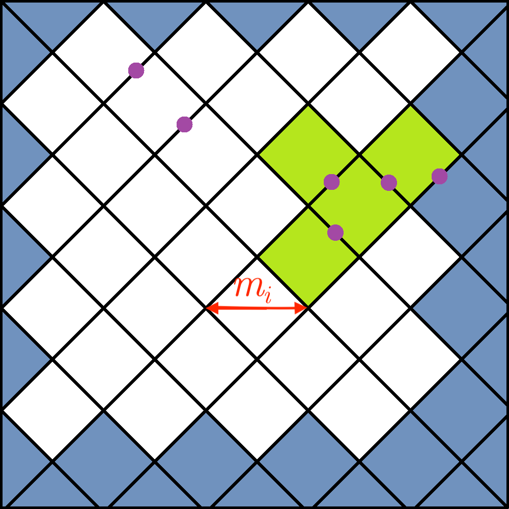
Figure 3.2: An example of execution of Algorithm 2. Black lines represent lattice pixels. The blue diamonds are included in $B$ because they are adjacent to the border of the square. The purple dots represent black pixels in the lattice. The green diamonds are added to $B$ during the BFS because their fences contain black pixels. The white diamonds remain in $A$.

Our nonadaptive algorithm reads all pixels in each sampled square. Our adaptive algorithm further partitions each square into diamonds, as shown in Figure 3.2. It queries all pixels on the diamond lattice and then adaptively tries to catch a witness (that is, a small connected component) in one of the diamonds, using the lattice structure. (We could have partitioned into squares again, but partitioning into diamonds makes the proof cleaner and saves a constant factor in the analysis.)

The Lower Bound.

We also prove the first nontrivial lower bound for testing connectedness of images. Note that all nontrivial properties have query complexity $\Omega(1/{\epsilon})$, even for adaptive testers. In particular, for connectedness, this is the number of queries needed to distinguish between the white image and an image, where we color black a random subset of size ${\epsilon}n^{2}$ of the set of pixels with both coordinates divisible by 3. By standard arguments, it implies a lower bound of $\Omega(1/{\epsilon})$. Some properties of images, such is being a halfplane, can be tested nonadaptively (with 1-sided error) with $O(1/{\epsilon})$ queries [6]. We show that it is impossible for connectedness.

Theorem 1.2.

Every nonadaptive (1-sided error) ${\epsilon}$-tester for connectedness of images must query $\Omega(\frac{1}{{\epsilon}}\log\frac{1}{{\epsilon}})$ pixels (for some family of images).

Every 1-sided error tester must catch a witness of disconnectedness in order to reject. This witness could include a connected component completely surrounded by white pixels. The difficulty for proving hardness is that, unlike in the case of finding a witness for disconnectedness of graphs, the algorithm does not have to read the whole connected component. Instead, it is sufficient to find a closed white loop with a black pixel inside it (and another black pixel outside it). As we discussed, it is sufficient for an algorithm to look for witnesses inside relatively small squares (specifically, squares with side length $O(1/{\epsilon})$), since adding a grid around such squares, as shown in Figure 1.2, would change $O({\epsilon}n^{2})$ pixels. But no matter how you had a witness inside such a square, it can be easily captured with $O(1/{\epsilon})$ queries if the border of the square is white.

To overcome this difficulty, we consider a checkerboard-like pattern with white squares replaced by many parallel lines, called bridges, with one white (disconnecting) pixel positioned randomly on each bridge. See Figure 4.1. To catch a white border around a connected component, a tester has to query all disconnecting pixels of at least one square. To make this difficult, we hide the checkerboard pattern inside a randomly positioned interesting window. The sizes of interesting windows and their positions are selected so that the tester cannot effectively reuse queries needed to succeed in catching the disconnecting pixels in each interesting window.

1.2 Other Related Work

In addition to [12], connectedness testing and approximating the number of connected components in graphs in sublinear time was explored in [10, 5, 4]. Other property testing tasks studied in the pixel model of images, the model considered in this paper, include testing whether an image is a half-plane [19], convexity [19, 7, 6], and image partitioning properties [14]. Early implementations and applications to vision were provided in [14, 15, 16, 18]. Finally, general classes of matrix properties were investigated, including matrix-poset properties [11], earthmover resilient properties [2], hereditary properties [1], and classes of matrices that are free of specified patterns [3].

Testing connectedness has also been studied by Ron and Tsur [20] with a different input representation suitable for testing sparse images.

2 Definitions and Notation

We use $[0..{n})$ to denote the set of integers $\{0,1,\ldots,n-1\}$ and $[n]$ to denote $\{1,2,\ldots,n\}$. By $\log$ we mean the logarithm base 2.

Image Representation.

We represent an image by an $n\times n$ binary matrix $M$ of pixel values, where 0 denotes white and 1 denotes black. The object is a subset of $[0..{n})^{2}$ corresponding to black pixels; namely, $\{(i,j)\mid M[i,j]=1\}$. The border of the image is the set $\{(i,j)\in[0..{n})^{2}\mid i\in\{0,n-1\}\text{ or }j\in\{0,n-1\}\}$.

Property Testing Definitions.

A property ${\mathcal{P}}$ is a set of images. The absolute distance from an image $M$ to a property ${\mathcal{P}}$, denoted $Dist(M,{\mathcal{P}}),$ is the smallest number of pixels in $M$ that need to be modified to get an image in ${\mathcal{P}}.$ The (relative) distance between an $n\times n$ image $M$ and a property ${\mathcal{P}}$ is $dist(M,{\mathcal{P}})=Dist(M,{\mathcal{P}})/n^{2}.$ We say that $M$ is ${\epsilon}$-far from ${\mathcal{P}}$ if $dist(M,{\mathcal{P}})\geq{\epsilon}$; otherwise, $M$ is ${\epsilon}$-close to ${\mathcal{P}}.$

3 Adaptive and Nonadaptive Property Testers for Connectedness

In this section, we present our testers for connectedness, proving Theorem 1.1. Both testers use the same top-level procedure, described in Algorithm 1. First, it samples random pixels to ensure that a black pixel is found. It will be used later to certify non-connectedness by producing a black pixel and an isolated black component. Then Algorithm 1 considers a logarithmic number of partitions of the image into subimages of the same size. For each partition, it samples a carefully selected number of these subimages and tests them for border connectedness (see Definition  1.1). This is where the two algorithms diverge. The nonadaptive algorithm tests for border connectedness using the subroutine Exhaustive-Square-Tester which queries all pixels in the sampled square and determines exactly if the square is border connected. The adaptive algorithm uses subroutine Diagonal-Square-Tester (Algorithm 2). If the top-level procedure finds a subimage that violates border connectedness and a black pixel outside that subimage, it rejects; otherwise, it accepts.

To simplify the analysis of the algorithm, we assume that $n-1$ and $1/{\epsilon}$ are powers of $2$. Next, we define terminology used to describe the partitions considered by Algorithm 1.

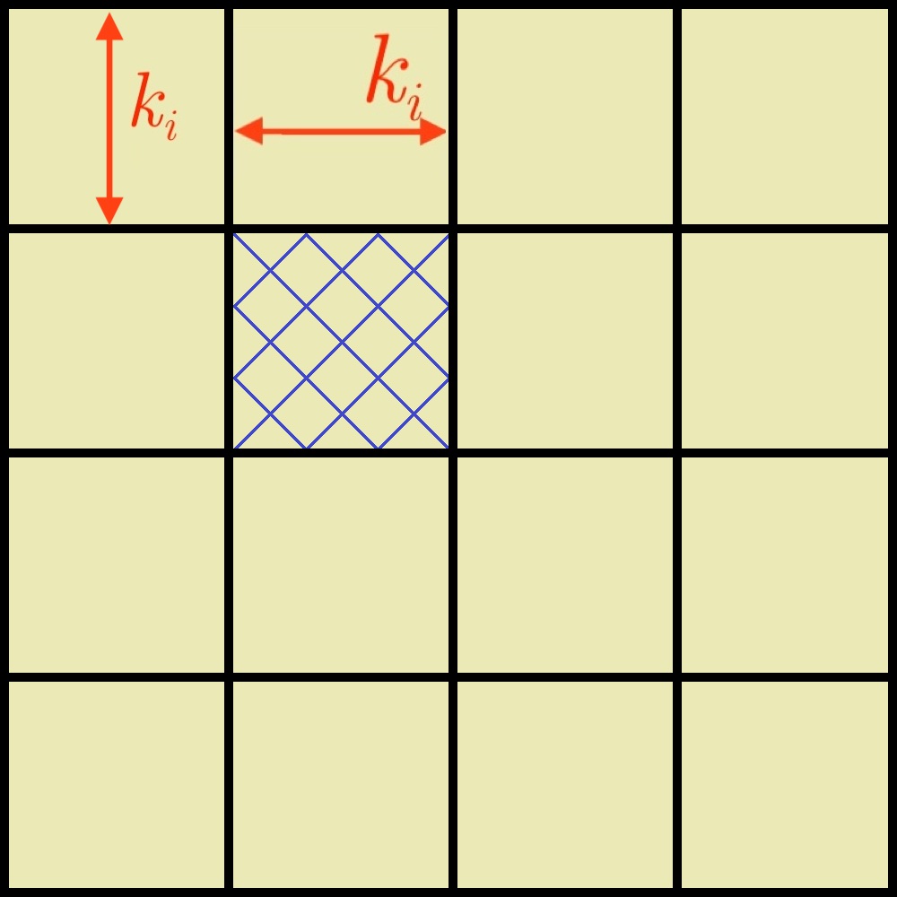
Figure 3.1: An illustration to Definition 3.1: black lines consist of grid pixels; the 16 yellow $k_{i}\times k_{i}$ squares represent squares of $S_{i}$. One of the squares includes diagonal lattice pixels from Definition 3.3 that are used in Algorithm 2.

Definition 3.1 (Grid pixels, squares of different levels, witnesses).

For $i\in[0..{\log\frac{1}{{\epsilon}}})$, let $k_{i}=\frac{4}{{\epsilon}}\cdot 2^{-i}-1$. Call $(x,y)$ a grid pixel of level $i$ if $(k_{i}+1)|x$ or $(k_{i}+1)|y$.

For all coordinates $u,v$, which are divisible by $k_{i}+1$,

the $k_{i}\times k_{i}$ subimage that consists of pixels $[k_{i}]^{2}+(u,v)$ is called a square of level $i$. The set of all squares of level $i$ is denoted ${\cal{S}}_{i}$. Boundary pixels of a square of level $i$ are the pixels of the square which are adjacent to the grid pixels of level $i$. A square of any level that violates property ${\mathcal{C}}^{\prime}$ (see Definition 1.1) is called a witness.

input : parameter ${\epsilon}\in(0,1)$ ; access to a $n\times n$ binary matrix $M$.

1 Query $\frac{4}{{\epsilon}}$ pixels uniformly at random with replacement.

2 for $i=0$ to $\log\frac{1}{{\epsilon}}-1$ do

3 Repeat $2^{i+1}$ times:

1. Sample a uniformly random square $s$ of level $i$ (see Definition 3.1) and let $[k_{i}]^{2}+(u,v)$ be the set of its pixels.

2. Run the border-connectedness subroutine with inputs $i,u,v$: if the tester is nonadaptive, use Exhaustive-Square-Tester; otherwise, use Diagonal-Square-Tester (Algorithm 2).

      If the subroutine rejects and Step 1 detected a black pixel outside $s$, reject.

     

     4 Accept.

Algorithm 1 ${\epsilon\emph{-tester}}$ for connectedness.

3.1 Effective Local Cost and the Structural Lemma

In this section, we state and prove the main structural lemma (Lemma 3.3) used in the analysis of Algorithm 1. It relates the distance to connectedness to the properties of individual squares, defined next.

Definition 3.2 (Local cost and effective local cost).

For a level $i$, consider a square $s\in{\cal{S}}_{i}$. The local cost of $s$ is $lc(s)=Dist(s,{\mathcal{C}}^{\prime})$. The effective local cost of $s$ is $elc(s)=\min(2k_{i},lc(s))$.

Next we state and prove two claims used in the proof of Lemma 3.3.

Claim 3.1.

For any square $s$ of level $i\in[0..{\log\frac{1}{{\epsilon}}-1})$, let $ch(s)$ denote the set of its $4$ children (i.e., squares of level $i+1$ inside it). Then $lc(s)\leq elc(s)+\sum\nolimits_{q\in ch(s)}lc(q)$.

Proof.

If $lc(s)\leq 2k_{i}$ then $elc(s)=lc(s)$. Since all costs are nonnegative, the inequality in 3.1 becomes trivial.

Now assume that $lc(s)>2k_{i}$. Then $elc(s)=2k_{i}$. We can modify $\sum\nolimits_{q\in ch(s)}lc(q)$ pixels in $s$ so that all its children satisfy the property ${\mathcal{C}}^{\prime}$. (Note that here ${\mathcal{C}}^{\prime}$ is the set of $k_{i}\times k_{i}$ (sub)images.) Then we can make black all pixels of $s$ that partition it into its children, i.e., pixels $\{(x,y)\mid x=\frac{k_{i}+1}{2}$ or $y=\frac{k_{i}+1}{2}\}$. There are at most $2k_{i}$ such pixels, and after this modification $s$ will satisfy ${\mathcal{C}}^{\prime}$. Hence, $lc(s)\leq elc(s)+\sum\nolimits_{q\in ch(s)}lc(q)$. ∎

Claim 3.2 (Distance to Border Connectedness).

Let $s$ be a $k\times k$ image. Then

$$Dist(s,{\mathcal{C}}^{\prime})\leq\frac{k^{2}}{4}.$$

Proof.

If $s$ contains at most $\frac{k^{2}}{4}$ black pixels, we can make all of them white, i.e., modify at most $\frac{k^{2}}{4}$ pixels and obtain an image that satisfies ${\mathcal{C}}^{\prime}$. Now consider an image $s$ with more than $\frac{k^{2}}{4}$ black pixels, i.e., with less than $\frac{3k^{2}}{4}$ white pixels. Partition all pixels of $s$ into $3$ groups such that group $i\in\{0,1,2\}$ contains all pixels $(x,y)$, where $y\equiv i\pmod{3}$. Making all pixels of one group black produces an image that satisfies ${\mathcal{C}}^{\prime}$. By averaging, at least one group has less than $\frac{k^{2}}{4}$ white pixels. Making all these white pixels black results in an image that satisfies ${\mathcal{C}}^{\prime}$. This completes the proof. ∎

Lemma 3.3 (Structural Lemma).

Let $M$ be an $n\times n$ image that is ${\epsilon}$-far from ${\mathcal{C}}$. Then the sum of effective local costs of all squares of all levels inside $M$ is at least $\frac{{\epsilon}n^{2}}{2}$.

Proof.

To obtain a connected image, we can make all the $\frac{{\epsilon}n^{2}}{2}$ grid pixels of level $0$ black and modify pixels inside every square of $\mathcal{S}_{0}$ to ensure it satisfies the property ${\mathcal{C}}^{\prime}$. Thus,

$$\sum\nolimits_{s\in\mathcal{S}_{0}}lc(s)\geq Dist(M,{\mathcal{C}})-\frac{{\epsilon}n^{2}}{2}\geq\frac{{\epsilon}n^{2}}{2}.$$

Consequently, it suffices to show that $\sum\nolimits_{i=0}^{\log\frac{1}{{\epsilon}}-1}\sum\nolimits_{s\in\mathcal{S}_{i}}elc(s)\geq\sum\nolimits_{s\in\mathcal{S}_{0}}lc(s)$.

Fix a level $i$ and a square $s\in\mathcal{S}_{i}$. Let $desc(s,j)$ denote the set of all squares of level $j\geq i$ inside $s$. (In particular, $desc(s,i)$ contains only $s$.) We will prove by induction that for all integer $j\in[i,\log\frac{1}{{\epsilon}}-1),$

$$lc(s)\leq\sum_{h=i}^{j}\sum\nolimits_{q\in desc(s,h)}elc(q)+\sum\nolimits_{q\in desc(s,j+1)}lc(q).$$ (1)

For $j=i$ (base case), the inequality in (1) holds since it is equivalent to the statement in Claim 3.1. Assume that (1) holds for $j=m$, that is,

$$lc(s)\leq\sum_{h=i}^{m}\sum\nolimits_{q\in desc(s,h)}elc(q)+\sum\nolimits_{q\in desc(s,m+1)}lc(q).$$

We will prove (1) holds for $j=m+1$. By Claim 3.1,

$$lc(q)\leq elc(q)+\sum\nolimits_{f\in ch(q)}lc(f).$$

Thus,

$$\sum\nolimits_{q\in desc(s,m+1)}lc(q)\leq\sum\nolimits_{q\in desc(s,m+1)}elc(q)+\sum\nolimits_{q\in desc(s,m+2)}lc(q)$$

and

$$lc(s) \leq\sum_{h=i}^{m}\sum\nolimits_{q\in desc(s,h)}elc(q)+\sum\nolimits_{q\in desc(s,m+1)}lc(q)$$

$$\leq\sum_{h=i}^{m+1}\sum\nolimits_{q\in desc(s,h)}elc(q)+\sum\nolimits_{q\in desc(s,m+2)}lc(q),$$

completing the inductive argument.

By (1) applied with $j=\log\frac{1}{{\epsilon}}-2$, we get that for every square $s$ of level $i$,

$$lc(s) \leq\sum_{h=i}^{\log\frac{1}{{\epsilon}}-2}\sum\nolimits_{q\in desc(s,h)}elc(q)+\sum\nolimits_{q\in desc(s,\log\frac{1}{{\epsilon}}-1)}lc(q)$$

$$=\sum_{h=i}^{\log\frac{1}{{\epsilon}}-1}\sum\nolimits_{q\in desc(s,h)}elc(q),$$ (2)

where the final equality holds because in every square of level $i=\log\frac{1}{{\epsilon}}-1$, we have $k_{i}=7$, and consequently, by 3.2, the local cost is at most $\frac{7^{2}}{4}<2\cdot 7$, i.e., it is equal to the effective local cost of that square. Summing up (2) for all squares in $\mathcal{S}_{0}$, we get

$$\sum\nolimits_{s\in\mathcal{S}_{0}}lc(s)\leq\sum\nolimits_{s\in\mathcal{S}_{0}}\sum\nolimits_{h=0}^{\log\frac{1}{{\epsilon}}-1}\sum\nolimits_{q\in desc(s,h)}elc(q)=\sum\nolimits_{h=0}^{\log\frac{1}{{\epsilon}}-1}\sum\nolimits_{s\in\mathcal{S}_{h}}elc(s),$$

where the last equality is obtained by switching the order of summations and rearranging the second summation in terms of levels. ∎

3.2 Testing Border-Connectedness

In this section, we state and analyze our adaptive border connectedness subroutine after defining the concepts used in it. We state the guarantees of both border connectedness subroutines in Lemma 3.4.

For the adaptive subroutine, we partition the square into diamonds and fences surrounding them, as described in Definition 3.3. The subroutine queries all pixels on the fences and categorizes diamonds into those whose black pixels are potentially connected to the border (set $B$ in Algorithm 2) and those whose black pixels are definitely not (set $A$ in Algorithm 2). Then it tries to find a black pixel in a diamond from set $A$ or (using BFS) an isolated black component in diamonds from set $B$. Observe that either of the two provides evidence that the square is not border-connected.

Definition 3.3 (Diagonal lattice pixels, diamonds and fences).

For a fixed value of $i$, consider a square $s$ in $\mathcal{S}_{i}$. Let $m_{i}$ be the largest odd integer less than or equal to $\lceil\sqrt{k_{i}/\log k_{i}}\rceil$. Diagonal lattice pixels of the square is the set of pixels $L=\{(x,y)\in s\mid m_{i}|(x+y)$ or $m_{i}|(x-y)\}$. Let $D$ be a $k_{i}\times k_{i}$ image whose pixels with coordinates from $[k_{i}]^{2}-L$ are black and the remaining pixels are white. A set of pixels of the square whose corresponding pixels in $D$ form a connected component is called a diamond of the square. A set of all diagonal lattice pixels that have some neighbouring pixel(s) from a particular diamond is called the fence of that diamond.

Note that lattice pixels are not part of any diamond. Moreover, some diamonds are partial (those that have pixels from the border of the square.)

input : parameters $i$, $u$ and $v$; access to an $n\times n$ matrix $M$.

Let $s$ be a square of level $i$ that consists of pixels $[k_{i}]^{2}+(u,v)$ and $m_{i}$ be the largest odd integer less than or equal to $\lceil\sqrt{k_{i}/\log k_{i}}\rceil$.

1 Query all the diagonal lattice pixels of $s$ (see Definition 3.3).

2 Initialize $B$ to be the set of all diamonds of $s$ that contain a border pixel of $s$. Initialize $A$ to be the set of the remaining diamonds of $s.$

3 While $\exists d_{1}\in B$ and $\exists d_{2}\in A$ such that $d_{1}$ and $d_{2}$ have a black pixel in the common portion of their fences, move $d_{2}$ from $A$ to $B$.

4 Repeat $\frac{1}{2}k_{i}m_{i}$ times:

1. Sample a uniform pixel $p$ from the square $s$.

If $p$ is a black pixel from a diamond in $A$ or its fence, reject.

If $p$ is a black pixel from a diamond in $B$, pick a natural number $x\in[k_{i}^{2}]$ from the distribution with the probability mass function $f(j)=\frac{1}{j(j+1)}$ for all $j\in[k^{2}_{i}-1]$ and $f(j)=\frac{1}{j}$ for $j=k^{2}_{i}$. (Observe that $\Pr(x\geq j)=\frac{1}{j}$ for all $j\in[k_{i}^{2}]$.)

Starting from $p$, perform a BFS of its connected component, halting if $x+1$ black pixels in $p$’s component are discovered or a black pixel on the border of square $s$ is reached. If the BFS halts after discovering at most $x$ black pixels, none of which are on the border of $s,$ reject.

5 Accept.

Algorithm 2 Border-connectedness subroutine Diagonal-Square-Tester.

Recall from Definition 3.1 that a witness is a square of one of the levels that violates border-connectedness.

Lemma 3.4.

Fix level $i\in[0..{\log\frac{1}{{\epsilon}}})$. Let $s\in\mathcal{S}_{i}$ be a witness that consists of pixels $[k_{i}]^{2}+(u,v)$. A border-connectedness subroutine called by Algorithm 1 rejects $s$ with probability at least $\frac{elc(s)\cdot\alpha}{2k_{i}}$, where $\alpha=1$ for Exhaustive-Square-Tester and $\alpha=1-e^{-1}$ for Diagonal-Square-Tester.

Proof.

Exhaustive-Square-Tester determines that $s$ is a witness with probability $1\geq\frac{elc(s)}{2k_{i}}\cdot 1$.

Now we prove the statement for Diagonal-Square-Tester. Let $A$ and $B$ be defined as in Algorithm 2 after Step 3. Let $a$ be the number of black pixels in all the diamonds of the set $A$ and on the fences of those diamonds. Let $b$ be the number of connected components of the image graph that are formed by black pixels in all the diamonds in the set $B$ and in their fences and that contain no pixels on the border of $s$. Next, we prove that

$$bm_{i}+a\geq lc(s)\geq elc(s).$$ (3)

The second inequality in (3) holds by Definition 3.2. To prove the first, we will show how to obtain a square in ${\mathcal{C}}^{\prime}$ by modifying at most $bm_{i}+a$ pixels in $s$.

We claim that we can connect all $b$ connected components to each other and to the border of the square by modifying at most $bm_{i}$ pixels. To see this, notice that any two black pixels in the same diamond can be connected to each other by changing less than $m_{i}$ pixels (by taking any Manhattan-distance shortest path between the two pixels and making it all black). To prove the claim, we can connect the $b$ connected components to the border of the square in the order their diamonds were added to $B$ by the algorithm. The initial diamonds placed in $B$ have at least one pixel on the border of the square, so their connected components can be directly connected to the border (using at most $m_{i}$ pixels per connected component). Now assume that we already connected to the border all components that have pixels in the diamonds added to $B$ so far. When the algorithm moves some diamond $d_{2}$ from $A$ to $B$, it is done because there is already a diamond $d_{1}$ in $B$ such that $d_{1}$ and $d_{2}$ have a black pixel $\beta$ in the common portion of their fences. Then $\beta$ must be already connected to the border. If there are any connected components in $d_{2}$ that are not connected to the border yet, we can fix that by connecting them to $\beta$ (using at most $m_{i}$ pixels per connected component). We proceed like this until all $b$ connected components of the diamonds that were added to $B$ by the algorithm are connected to the border of the square. At this point, we have changed at most $bm_{i}$ pixels.

Recall that we have $a$ black pixels in all the diamonds of the set $A$ and on the fences of those diamonds. We make all of them white. After these at most $bm_{i}+a$ modifications to $s$, we obtain a square in ${\mathcal{C}}^{\prime}$. Thus, (3) holds.

Observe that for $x\in[0,1]$,

$$x\geq 1-e^{-x}\geq x(1-e^{-1})>x/2.$$ (4)

Consider one iteration of Step 2 of Algorithm 2. Let $E_{1}$ be the event that $p$ is one of the $a$ black pixels in the diamonds of the set $A$. Let $CC$ denote the set of the $b$ connected components from the diamonds of the set $B$. Let $E_{2}$ be the event that $p$ is in one of the connected components in $CC$ and that its connected component is completely discovered by the BFS in Step 2b. Then the probability that one iteration of Step 2 of Algorithm 2 rejects square $s$ is equal to $\Pr[E_{1}]+\Pr[E_{2}]$. Since $p$ is chosen uniformly from a square of size $k_{i}\times k_{i}$,

$$\Pr[E_{1}]=\frac{a}{k^{2}_{i}}.$$

Since $p$ and $x$ are chosen independently,

$$\Pr[E_{2}]=\sum_{C\in CC}\Pr_{p}[p\in C]\cdot\Pr_{x}[x\geq|C|]=\sum_{C\in CC}\frac{|C|}{k^{2}_{i}}\cdot\frac{1}{|C|}=\sum_{C\in CC}\frac{1}{k^{2}_{i}}=\frac{b}{k^{2}_{i}}.$$

Then, by (3) and (4) and since $\frac{elc(s)}{2k_{i}}\leq 1$ by Definition 3.2, the probability that all $\frac{1}{2}k_{i}m_{i}$ iterations of Step 2 of Algorithm 2 proceed without rejecting is

$$\left(1-\frac{a+b}{k^{2}_{i}}\right)^{\frac{1}{2}k_{i}m_{i}}\leq e^{-\frac{a+b}{2k_{i}}\cdot m_{i}}\leq e^{-\frac{a+bm_{i}}{2k_{i}}}\leq e^{{-\frac{elc(s)}{2k_{i}}}}\leq 1-\frac{elc(s)}{2k_{i}}(1-e^{-1}).$$

Therefore, Algorithm 2 rejects $s$ with probability at least

$$\frac{elc(s)}{2k_{i}}(1-e^{-1}),$$

completing the proof of Lemma 3.4

∎

3.3 Proof of Theorem 1.1

In this section, we use Lemmas 3.3 and 3.4 to complete the analysis of our connectedness tester and the proof of Theorem 1.1.

Algorithm 1 always accepts connected images, since it sees no violation of ${\mathcal{C}}^{\prime}$ in Step 1b. Consider an image $M$ that is ${\epsilon}$-far from connectedness. Fix level $i\in\big{[}0..\log\frac{1}{{\epsilon}}\big{)}$ and one iteration of Step 1 of Algorithm 1. Let $s$ be a square of level $i$ and $E_{s}$ be the event that,

in this iteration, $s$ is selected in Step 1a and rejected by the subroutine in Step 1b. Observe that for every $i\in[0..{\log\frac{1}{{\epsilon}}})$, there are $\frac{n^{2}}{k_{i}^{2}}$ squares in $\mathcal{S}_{i}$. By Lemma 3.4,

$$\Pr[E_{s}]\geq\frac{k_{i}^{2}}{n^{2}}\cdot\frac{\alpha\cdot elc(s)}{2k_{i}}=\frac{\alpha\cdot k_{i}\cdot elc(s)}{2n^{2}}.$$

Let $E$ be the event that,

in this iteration, the subroutine in Step 1b rejects. Since events $E_{s}$ are disjoint and $E=\bigcup_{s\in\mathcal{S}_{i}}E_{s},$

$$\Pr[E]=\sum_{s\in\mathcal{S}_{i}}\Pr[E_{s}]\geq\frac{\alpha\cdot k_{i}}{2n^{2}}\cdot\sum_{s\in\mathcal{S}_{i}}elc(s).$$

Let $\mathcal{S}$ be the set of squares of all levels $i\in[0..\log\frac{1}{{\epsilon}})$. By independence and Lemma 3.3, the overall probability that the subroutine accepts in all iterations is at most

$$\prod_{i\in[0..{\log\frac{1}{{\epsilon}}})}\left(1-\frac{\alpha\cdot k_{i}}{2n^{2}}\cdot\sum_{s\in\mathcal{S}_{i}}elc(s)\right)^{2^{i+1}} \leq\prod_{i\in[0..{\log\frac{1}{{\epsilon}}})}\exp\left(-\frac{\alpha}{2}\cdot\frac{4}{{\epsilon}n^{2}2^{i}}\cdot\sum_{s\in\mathcal{S}_{i}}elc(s)\cdot 2^{i+1}\right)$$

$$=\exp\left(-\frac{4\alpha}{{\epsilon}n^{2}}\cdot\sum_{s\in\mathcal{S}}els(s)\right) \leq\exp\left(-\frac{4\alpha}{{\epsilon}n^{2}}\cdot\frac{{\epsilon}n^{2}}{2}\right)=e^{-2\alpha}.$$

Therefore, the probability that Algorithm 1 detects at least one witness is at least $1-e^{-2\alpha}$. Since at least an ${\epsilon}$ fraction of pixels in $M$ are black and every square of every level contains at most $\frac{16}{{\epsilon}^{2}}\leq\frac{{\epsilon}n^{2}}{4}$ pixels (recall that $n\geq 8{\epsilon}^{-3/2}$ in the premise of Theorem 1.1), the probability that Algorithm 1 detects a black pixel outside of that witness in Step 1 is at least $1-(1-\frac{3{\epsilon}}{4})^{\frac{4}{{\epsilon}}}>1-e^{-3}$. Thus, for both values of $\alpha$, the probability that Algorithm 1 rejects $M$ is at least

$$(1-e^{-3})(1-e^{-2\alpha})\geq 2/3,$$

completing the analysis of the success probability of Algorithm 1.

Query Complexity.

We prove that Algorithm 1 has query complexity $O(\frac{1}{{\epsilon}^{2}})$ if it uses Exhaustive-Square-Tester as a subroutine. Algorithm 1 samples $2^{i+1}$ squares of level $i\in[0..\log\frac{1}{{\epsilon}})$ and, for each sampled square, it calls Exhaustive-Square-Tester which makes $(\frac{4}{{\epsilon}}\cdot 2^{-i}-1)(\frac{4}{{\epsilon}}\cdot 2^{-i}-1)<\frac{16}{{\epsilon}^{2}2^{2i}}$ queries in each sampled square of level $i$. Thus, the query complexity of Algorithm 1 is

$$\sum\nolimits_{i=0}^{\log\frac{1}{{\epsilon}}}2^{i+1}\cdot\frac{16}{{\epsilon}^{2}2^{2i}}<\sum\nolimits_{i=0}^{\log\frac{1}{{\epsilon}}}\frac{32}{{\epsilon}^{2}2^{i}}=O\left(\frac{1}{{\epsilon}^{2}}\right).$$

When Algorithm 1 uses Diagonal-Square-Tester, it queries at most $\frac{2k_{i}^{2}}{m_{i}}$ diagonal lattice pixels inside each square of level $i$ (in Step 2 of the subroutine). After that, in Step 2 of the subroutine, it selects $\frac{1}{2}{k_{i}m_{i}}$ pixels and a number $x\in[k_{i}^{2}]$ from the specified distribution and then makes at most $4x$ queries for each selected pixel. Observe that $\operatorname*{\mathbb{E}}(x)=O(\log k_{i})$. Thus, the expected number of queries inside a square of level $i$ is at most $\frac{2k_{i}^{2}}{m_{i}}+\frac{1}{2}k_{i}m_{i}\cdot 4\cdot O(\log k_{i})=O(k_{i}^{3/2}\sqrt{\log k_{i}})$. The expected total number of queries is $\sum\nolimits_{i=0}^{\log(1/{\epsilon})}O(k_{i}^{3/2}\sqrt{\log k_{i}})\cdot 2^{i+1}=O({\epsilon}^{-3/2}\sqrt{\log\frac{1}{{\epsilon}}})$.

By standard arguments, the adaptive version of Algorithm 1 can be converted to an algorithm that makes asymptotically the same number of queries in the worst case, and has the same accuracy guarantee and running time.

Running Time.

The time complexity of Step 1a and Step 2 of Algorithm 1 is $O(\frac{1}{{\epsilon}})$. Therefore, the total time complexity of Algorithm 1 is $O(\frac{1}{{\epsilon}})$+time complexity of Step 1b. In Step 1b, Algorithm 1 uses either Exhaustive-Square-Tester or Diagonal-Square-Tester. Both of them perform a breadth first search within each sampled square. Breadth first search is linear in the sum of the number of edges and the number of nodes of the graph. Every pixel of a sampled square has at most $4$ neighboring pixels. Thus, the number of edges in the image graph of every sampled square is linear in the number of pixels inside it and the time complexity of Step 1b is linear in the number of all queried pixels, i.e., $O(\frac{1}{{\epsilon}^{2}})$ for Exhaustive-Square-Tester and $O({\epsilon}^{-3/2}\sqrt{\log(1/{\epsilon})})$ for Diagonal-Square-Tester. This completes the proof of the theorem.

4 Lower Bound for Testing Connectedness

In this section, we give a lower bound on the query complexity of testing connectedness, proving Theorem 1.2. We use the standard set up of constructing a distribution $\mathcal{N}$ on ${\epsilon}$-far inputs such that every deterministic nonadaptive algorithm that makes $q\leq\frac{c}{{\epsilon}}\log\frac{1}{{\epsilon}}$ queries (for some constant $c$) has probability of error greater than 1/3. By Yao’s Principle [22], it is sufficient to prove Theorem 1.2.

4.1 Construction of $\mathcal{N}$

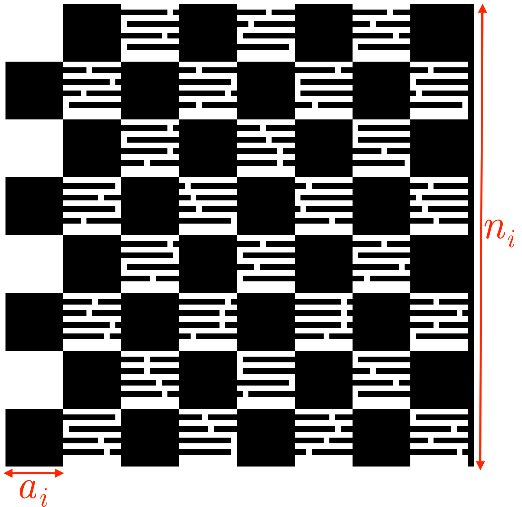
Figure 4.1: Our construction of $\mathcal{N}$: an interesting window together with a column of black pixels immediately to the right of it. All other pixels in the constructed image are white.

The construction is parameterized by $n$ and the proximity parameter ${\epsilon}$. It gives a distribution supported on $(n+1)\times(n+1)$ images that are ${\epsilon}$-far from connectedness. We assume that ${\epsilon}$ is sufficiently small and that $n>\frac{1}{16}(\frac{1}{{\epsilon}})^{5/8}.$

We also assume that $n$ is a power of $2$ and $1/{\epsilon}$ is an even power of $2$ and that both of them are sufficiently large, so that all indices in our construction are integer. (See also Footnote 2 for the discussion of integrality issues.) Our construction starts by selecting a level. The indices of the levels range from the low index $\ell=\frac{1}{8}\log\frac{1}{{\epsilon}}$ to the high index $h=\frac{1}{4}\log\frac{1}{{\epsilon}}$. For all $i\in\{\ell,\ell+1,\dots,h\}$, define $a_{i}=2^{i}$ and $n_{i}=16\cdot\sqrt{\epsilon}\cdot n\cdot a_{i}=\sqrt{\epsilon}\cdot n\cdot 2^{i+4}$. First, we pick a uniformly random integer $i\in\{\ell,\ell+1,\dots,h\}$. Consider the $n\times n$ image resulting from removing the last row and the last column of the $(n+1)\times(n+1)$ image. We partition this $n\times n$ image into $(\frac{n}{n_{i}})^{2}$ squares with side length $n_{i}$ called windows of level $i$; that is, each window of level $i$ is an $n_{i}\times n_{i}$ subimage. We pick one of the windows of level $i$ uniformly at random and call it an interesting window. We make the $n_{i}$ pixels immediately to the right of the interesting window black, representing a vertical black line segment, and all other pixels outside of the interesting window white.

Now we describe how to color the interesting window.

See Figure 4.1 for an illustration.

We fill the interesting window with a checkerboard pattern of squares of size $a_{i}\times a_{i}$ pixels. Inside each white checkerboard square that is not in the first column, number the rows starting from 0 and make every odd row, excluding the last, fully black, except for one randomly selected pixel for each row. The resulting $\frac{a_{i}}{2}-1$ black lines, each containing one white pixel, are called bridges. The white pixels on the bridges are called disconnecting pixels. We refer to each checkerboard square with the bridges as a bridge square.

The intuition behind the construction is the following. Each black checkerboard square is in its own connected component. However, to “catch” this connected component as a witness of disconnectedness, a tester would have to query all the disconnecting pixels in the bridge squares to the left and/or to the right of the black square. Since the positions of the disconnecting pixels are random, it would have to query $\Omega(a_{i}^{2})$ pixels in at least one relevant bridge square. Since the windows are selected at random, the algorithm would have to do it for many windows of each level. The key feature of our construction is that interesting windows of different levels are either disjoint or contained in one another, so potential witnesses for one window can’t significantly help with another.

4.2 Analysis of the Construction

We start by showing that all images in the support of $\mathcal{N}$ are far from connected.

Lemma 4.1.

Every image in the support of $\mathcal{N}$ is ${\epsilon}$-far from connected.

Proof.

There are $\frac{(n_{i}/a_{i})^{2}}{2}=128\epsilon n^{2}$ black regions, each one in a separate connected component except for the last $\frac{n_{i}/a_{i}}{2}=8\sqrt{\epsilon}\cdot n$ which are connected by the vertical line. Thus, the image graph has at least $128\cdot\epsilon n^{2}-8\sqrt{\epsilon}\cdot n$ connected components. Changing one pixel from white to black corresponds to adding a node of degree at most 4 to the image graph. This decreases the number of connected components by at most 3. Removing a pixel decreases the number of connected components by at most 1. Consequently, overall, we need to change at least $\frac{1}{3}{(128\epsilon n^{2}-8\sqrt{\epsilon}\cdot n)}$ pixels. This is at least $\epsilon n^{2}$ for sufficiently large $n$; in particular, it holds for $n>\frac{1}{16}(\frac{1}{{\epsilon}})^{5/8}$, which was our assumption in the beginning of Section 4.1. ∎

Next we show that if the number of queried pixels is small, then every 1-sided error deterministic algorithm detects a violation of connectedness in an image distributed according to $\mathcal{N}$ with insufficiently small probability.

Lemma 4.2.

Let $M$ be an image distributed according to $\mathcal{N}$. Fix a deterministic nonadaptive 1-sided error algorithm $\mathcal{A}$ for testing connectedness of images. Let $\bf Q$ be the set of pixels queried by $\mathcal{A}$ and let $q=|\bf Q|$. For sufficiently small constant $c>0$, if $q\leq\frac{c}{{\epsilon}}\log\frac{1}{{\epsilon}}$, then $\mathcal{A}$ detects a violation of connectedness in $M$ with probability less than $1/3$.

Proof.

We define an event $E$ that must happen in order for the algorithm ${\mathcal{A}}$ to succeed in finding a witness of disconnectedness in an image distributed according to $\mathcal{N}$. Then we show that the probability of $E$ is too small. To define $E$, we define a special group of pixels.

Definition 4.1 (A revealing set and event $E$).

Let $M$ be an image distributed according to $\mathcal{N}$. The set of all disconnecting pixels from one bridge square of $M$ is called a revealing set for the window containing the bridge square. Let $E$ denote the event that ${\bf Q}$ contains a revealing set for the interesting window of $M$.

Since the tester ${\mathcal{A}}$ has 1-sided error, it can reject only if it finds a violation of connectedness. In particular, for an image distributed according to $\mathcal{N}$, in order to succeed, it must find a revealing set for the interesting window of the image.

Claim 4.3.

If the number of queries $q\leq\frac{c}{{\epsilon}}\log\frac{1}{{\epsilon}}$ for sufficiently small constant $c$, then $\Pr[E]<1/3.$

Proof.

An important feature of our construction is that the largest bridge square is smaller than the smallest window. Indeed, the side length of the largest bridge square is $a_{h}=(\frac{1}{{\epsilon}})^{1/4}$, whereas the side length of the smallest window is $n_{\ell}=16\sqrt{{\epsilon}}\cdot(\frac{1}{{\epsilon}})^{1/8}n=16{\epsilon}^{3/8}n$. Thus, $a_{h}<n_{\ell}$ as long as $n>\frac{1}{16}(\frac{1}{{\epsilon}})^{5/8}$, as we assumed in the beginning of Section 4.1. The consequence of this feature and the fact that both $a_{i}$’s and $n_{i}$’s are powers of 2 is that each bridge square of level $i$ is contained in one window of level $j$ for all levels $i$ and $j.$

A (potential) bridge square of level $i\in\{\ell,\ell+1,\dots,h\}$ is covered if ${\bf Q}$ contains at least ${a_{i}^{2}}/8$ pixels from that square. A window of level $i$ is good if it contains a covered bridge square of level $j\geq i$; otherwise, it is bad. For each good window $w$, we pick a covered bridge square of the highest level contained in $w$ and call it the covered bridge square associated with $w$. All windows of the same level are associated with different covered bridge squares, because each bridge square is contained in exactly one window of a given level.

Let $G$ be the event that the interesting window in $M$ is good. Then, by the law of total probability,

$$\Pr[E]=\Pr[E\mid G]\cdot\Pr[G]+\Pr[E\mid\overline{G}]\cdot\Pr[\overline{G}]\leq\Pr[G]+\Pr[E\mid\overline{G}].$$

Next, we analyze event $G$. For every level $i\in\{\ell,\ell+1,\dots,h\},$ let $g_{i}$ be the number of good windows of level $i$ associated with covered bridge squares of level $i$ and let $t_{i}$ be the total number of good windows of level $i$. Then $g_{h}=t_{h}$ and $g_{i}=t_{i}-t_{i+1}$ for all $i\in[\ell,h-1].$ Observe that, for each level $i\in[\ell,h]$, the covered bridge squares associated with the good windows of level $i$ are distinct. By definition, each of them contributes at least ${a_{i}^{2}}/8$ towards ${\bf Q}$. Therefore, the number of all pixels in ${\bf Q}$ satisfies

$$q \geq\sum_{i=\ell}^{h}\frac{a^{2}_{i}g_{i}}{8}=\frac{1}{8}\left(\sum_{i=\ell}^{h-1}a^{2}_{i}(t_{i}-t_{i+1})+a_{h}^{2}t_{h}\right)=\frac{1}{8}\left(\sum_{i=\ell}^{h-1}4^{i}(t_{i}-t_{i+1})+4^{h}t_{h}\right)$$

$$\geq\frac{3}{32}\sum_{i=\ell}^{h}(4^{i}t_{i}).$$ (5)

Recall that $q\leq\frac{c}{{\epsilon}}\log\frac{1}{{\epsilon}}$, that the total number of levels is $h-\ell+1=\Theta(\log\frac{1}{{\epsilon}})$, and that the number of all windows for each level $i$ is $(\frac{n}{n_{i}})^{2}=\Theta(\frac{1}{4^{i}{\epsilon}}).$ Thus,

$$\Pr[G] =\frac{1}{h-\ell+1}\sum_{i=\ell}^{h}\frac{t_{i}}{(n/n_{i})^{2}}=\frac{1}{\Theta(\log(\frac{1}{{\epsilon}}))}\sum_{i=\ell}^{h}(t_{i}\cdot\Theta({4^{i}{\epsilon}}))=\frac{1}{\Theta(\frac{1}{{\epsilon}}\log(\frac{1}{{\epsilon}}))}\sum_{i=\ell}^{h}(4^{i}t_{i})$$

$$<\frac{q}{\Theta(\frac{1}{{\epsilon}}\log(\frac{1}{{\epsilon}}))}<1/6,$$

where Section 4.2 was used to obtain the first inequality, and the last inequality holds for sufficiently small constant $c$.

It remains to analyze $\Pr[E\mid\overline{G}],$ that is, the probability of $E$, given that the interesting window is bad. Consider a bad window of level $i\in\{\ell,\dots,h\}$. It has at most $q$ bridge squares that contain a queried pixel. Consider one of such bridge squares. Recall that this bridge square has $a_{i}/2-1$ bridges. Number these bridges using integers $1,2,\dots,a_{i}/2-1$. Let $x_{k}$ denote the number of pixels of Q on the bridge number $k\in[a_{i}/2-1]$ of the bridge square. Then the probability that this bridge square has a revealing set for the window is

$$\prod_{k=1}^{a_{i}/2-1}\frac{x_{k}}{a_{i}} \leq\left(\frac{1}{a_{i}/2-1}\cdot\sum_{k=1}^{a_{i}/2-1}\frac{x_{k}}{a_{i}}\right)^{a_{i}/2-1}\leq\left(\frac{a_{i}/8}{a_{i}/2-1}\right)^{a_{i}/2-1}\leq\left(\frac{1}{2}\right)^{a_{i}/2-1}$$

$$\leq 2(\sqrt{2})^{-\sqrt[8]{\frac{1}{{\epsilon}}}},$$

where the first inequality follows from the inequality between geometric and arithmetic means, the second inequality holds since $\sum_{k=1}^{a_{i}/2}x_{k}<a_{i}^{2}/8$, and the third inequality holds since ${\epsilon}$ is sufficiently small and, consequently, we can assume that the minimum value of $a_{i}$ is at least 4. By a union bound over all bridge squares in this window that contain a query,

$$\Pr[E\mid\overline{G}]\leq 2(\sqrt{2})^{-\sqrt[8]{\frac{1}{{\epsilon}}}}\cdot q\leq 2(\sqrt{2})^{-\sqrt[8]{\frac{1}{{\epsilon}}}}\cdot\frac{c}{{\epsilon}}\cdot{\log\frac{1}{{\epsilon}}<\frac{1}{6}},$$

for sufficiently small ${\epsilon}$ and constant $c$. Thus, $\Pr[E]\leq\Pr[G]+\Pr[E\mid\overline{G}]<\frac{1}{6}+\frac{1}{6}=\frac{1}{3},$ as claimed. This completes the proof of Claim 4.3. ∎

This concludes the proof of Lemma 4.2. ∎

Theorem 1.2 follows from Lemma 4.2.

References

- Alon et al. [2017] N. Alon, O. Ben-Eliezer, and E. Fischer. Testing hereditary properties of ordered graphs and matrices. In C. Umans, editor, 58th IEEE Annual Symposium on Foundations of Computer Science, FOCS 2017, Berkeley, CA, USA, October 15-17, 2017, pages 848–858. IEEE Computer Society, 2017. doi: 10.1109/FOCS.2017.83. URL https://doi.org/10.1109/FOCS.2017.83.
- Ben-Eliezer and Fischer [2018] O. Ben-Eliezer and E. Fischer. Earthmover resilience and testing in ordered structures. In R. A. Servedio, editor, 33rd Computational Complexity Conference, CCC 2018, June 22-24, 2018, San Diego, CA, USA, volume 102 of LIPIcs, pages 18:1–18:35. Schloss Dagstuhl - Leibniz-Zentrum für Informatik, 2018. doi: 10.4230/LIPIcs.CCC.2018.18. URL https://doi.org/10.4230/LIPIcs.CCC.2018.18.
- Ben-Eliezer et al. [2017] O. Ben-Eliezer, S. Korman, and D. Reichman. Deleting and testing forbidden patterns in multi-dimensional arrays. In I. Chatzigiannakis, P. Indyk, F. Kuhn, and A. Muscholl, editors, 44th International Colloquium on Automata, Languages, and Programming, ICALP 2017, July 10-14, 2017, Warsaw, Poland, volume 80 of LIPIcs, pages 9:1–9:14. Schloss Dagstuhl - Leibniz-Zentrum für Informatik, 2017. doi: 10.4230/LIPIcs.ICALP.2017.9. URL https://doi.org/10.4230/LIPIcs.ICALP.2017.9.
- Berenbrink et al. [2014] P. Berenbrink, B. Krayenhoff, and F. Mallmann-Trenn. Estimating the number of connected components in sublinear time. Inf. Process. Lett., 114(11):639–642, 2014. doi: 10.1016/j.ipl.2014.05.008. URL https://doi.org/10.1016/j.ipl.2014.05.008.
- Berman et al. [2014] P. Berman, S. Raskhodnikova, and G. Yaroslavtsev. -testing. In D. B. Shmoys, editor, Symposium on Theory of Computing, STOC 2014, New York, NY, USA, May 31 - June 03, 2014, pages 164–173. ACM, 2014. doi: 10.1145/2591796.2591887. URL https://doi.org/10.1145/2591796.2591887.
- Berman et al. [2019a] P. Berman, M. Murzabulatov, and S. Raskhodnikova. The power and limitations of uniform samples in testing properties of figures. Algorithmica, 81(3):1247–1266, 2019a.
- Berman et al. [2019b] P. Berman, M. Murzabulatov, and S. Raskhodnikova. Testing figures under the uniform distribution. Random Struct. Algorithms, 54(3):413–443, 2019b.
- Berman et al. [2022] P. Berman, M. Murzabulatov, and S. Raskhodnikova. Tolerant testers of image properties. ACM Transactions on Algorithms (TALG), 18(4):1–39, 2022.
- Berman et al. [2023] P. Berman, M. Murzabulatov, S. Raskhodnikova, and D. Ristache. Testing connectedness of images. In N. Megow and A. D. Smith, editors, Approximation, Randomization, and Combinatorial Optimization. Algorithms and Techniques, APPROX/RANDOM 2023, September 11-13, 2023, Atlanta, Georgia, USA, volume 275 of LIPIcs, pages 66:1–66:15. Schloss Dagstuhl - Leibniz-Zentrum für Informatik, 2023. doi: 10.4230/LIPICS.APPROX/RANDOM.2023.66. URL https://doi.org/10.4230/LIPIcs.APPROX/RANDOM.2023.66.
- Chazelle et al. [2005] B. Chazelle, R. Rubinfeld, and L. Trevisan. Approximating the minimum spanning tree weight in sublinear time. SIAM J. Comput., pages 1370–1379, 2005.
- Fischer and Newman [2007] E. Fischer and I. Newman. Testing of matrix-poset properties. Comb., 27(3):293–327, 2007. doi: 10.1007/s00493-007-2154-3. URL https://doi.org/10.1007/s00493-007-2154-3.
- Goldreich and Ron [2002] O. Goldreich and D. Ron. Property testing in bounded degree graphs. Algorithmica, 32(2):302–343, 2002.
- Goldreich et al. [1998] O. Goldreich, S. Goldwasser, and D. Ron. Property testing and its connection to learning and approximation. J. ACM, 45(4):653–750, 1998.
- Kleiner et al. [2011] I. Kleiner, D. Keren, I. Newman, and O. Ben-Zwi. Applying property testing to an image partitioning problem. IEEE Trans. Pattern Anal. Mach. Intell., 33(2):256–265, 2011.
- Korman et al. [2011] S. Korman, D. Reichman, and G. Tsur. Tight approximation of image matching. CoRR, abs/1111.1713, 2011.
- Korman et al. [2013] S. Korman, D. Reichman, G. Tsur, and S. Avidan. Fast-match: Fast affine template matching. In CVPR, pages 2331–2338. IEEE, 2013.
- Minsky and Papert [2017] M. Minsky and S. A. Papert. Perceptrons: An Introduction to Computational Geometry. The MIT Press, 09 2017. ISBN 9780262343930. doi: 10.7551/mitpress/11301.001.0001. URL https://doi.org/10.7551/mitpress/11301.001.0001.
- Paral et al. [2019] P. Paral, A. Chatterjee, and A. Rakshit. Vision sensor-based shoe detection for human tracking in a human–robot coexisting environment: A photometric invariant approach using dbscan algorithm. IEEE Sensors Journal, 19(12):4549–4559, 2019.
- Raskhodnikova [2003] S. Raskhodnikova. Approximate testing of visual properties. In S. Arora, K. Jansen, J. D. P. Rolim, and A. Sahai, editors, RANDOM-APPROX, volume 2764 of Lecture Notes in Computer Science, pages 370–381. Springer, 2003. ISBN 3-540-40770-7.
- Ron and Tsur [2014] D. Ron and G. Tsur. Testing properties of sparse images. ACM Trans. Algorithms, 10(4):17:1–17:52, 2014. doi: 10.1145/2635806. URL http://doi.acm.org/10.1145/2635806.
- Rubinfeld and Sudan [1996] R. Rubinfeld and M. Sudan. Robust characterizations of polynomials with applications to program testing. SIAM J. Comput., 25(2):252–271, 1996.
- Yao [1977] A. C. Yao. Probabilistic computation, towards a unified measure of complexity. In Proceedings of the Eighteenth Annual Symposium on Foundations of Computer Science, pages 222–227, 1977.