Hybrid Functional Maps for Crease-Aware Non-Isometric Shape Matching

Abstract

Non-isometric shape correspondence remains a fundamental challenge in computer vision. Traditional methods using Laplace-Beltrami operator (LBO) eigenmodes face limitations in characterizing high-frequency extrinsic shape changes like bending and creases. We propose a novel approach of combining the non-orthogonal extrinsic basis of eigenfunctions of the elastic thin-shell hessian with the intrinsic ones of the LBO, creating a hybrid spectral space in which we construct functional maps. To this end, we present a theoretical framework to effectively integrate non-orthogonal basis functions into descriptor- and learning-based functional map methods. Our approach can be incorporated easily into existing functional map pipelines across varying applications and is able to handle complex deformations beyond isometries. We show extensive evaluations across various supervised and unsupervised settings and demonstrate significant improvements. Notably, our approach achieves up to 15% better mean geodesic error for non-isometric correspondence settings and up to 45% improvement in scenarios with topological noise. Code will be made available upon acceptance.

Figure 1: We propose a novel approach of hybridizing the eigenbases from different linear operators for mappings between function spaces in deformable shape correspondence. While the Laplace-Beltrami operator (LBO) eigenbasis is robust to coarse isometric deformations, it fails to encapsulate extrinsic characteristics between shapes. In contrast, elastic basis functions [19] align with high curvature details but lack the robustness for coarse isometric matching. The proposed hybrid basis can be used as a drop-in replacement for the LBO basis functions in modern functional map pipelines, improving performance in near-isometric, non-isometric, and topologically noisy settings.

1 Introduction

Establishing dense correspondences between 3D shapes is a cornerstone for numerous computer vision and graphics tasks such as object recognition, character animation, and texture transfer. The complexity of this task varies significantly depending on the nature of the transformation a shape undergoes. Classic correspondence methods leverage the fact that rigid transformations can be represented in six degrees of freedom in $\mathbf{R}^{3}$ and preserve the Euclidean distance between pairs of points. Iterative closest point (ICP) [3], and its variations [24, 38], which alternate between transformation and correspondence estimation, are very popular due to their simplicity. In this setting, local extrinsic surface properties in the embedding space stay invariant under rigid transformations such that they can be used during optimization as features, for example, the change of normals. For the wider class of isometric deformations (w.r.t. the geodesic distance), the relative embedding of the shape can change significantly, and Euclidean distances between points may not be preserved. In this class, only intrinsic properties – those that do not depend on a specific embedding of the surface – stay invariant, and the correspondence problem becomes much harder due to the quadratic size of the solution space. For example, solving a quadratic assignment problem preserving geodesic distances [23] or heat kernel [49] is intrinsic by nature, but it is also an NP-hard problem.

In this context spectral shape analysis, a generalization of Fourier analysis to Riemannian manifolds, has emerged as a powerful tool for non-rigid correspondence by leveraging intrinsic shape structure. One popular method that takes advantages of this tool is functional maps, introduced by Ovsjanikov et al. [35], which synchronizes the eigenfunctions of the Laplace-Beltrami operator (LBO) through a low-dimensional linear change of basis. Numerous adaptations have led to advances in shape correspondence in recent years, for example, in both the learned supervised [27, 13] and unsupervised settings [43, 25, 9, 10, 48]; and while other basis choices have been proposed [34, 37, 19], almost all of these methods use the eigenfunctions of the Laplace-Beltrami operator (LBO) to span the to-be-mapped function spaces. One reason is that the LBO has been extensively studied, and the behavior of its eigenfunctions is well understood. For instance, the LBO’s eigenfunctions have a relatively consistent ordering and general invariance under isometric deformations. These understandings have been leveraged for efficient regularization [42] and coarse-to-fine optimization [33, 16]. Other basis sets have been studied and shown to be effective in specific cases [37, 11], but none are so generally applicable and flexible as the LBO eigenfunctions.

A known weakness of the LBO basis, which at the same time comes from its biggest strength, is the reduction to low-frequency information. This leads to efficient optimization and robustness to noise but also inaccuracy in small details. To counter this challenge, Hartwig et al. [19] proposed a basis emanating from the spectral decomposition of an elastic thin-shell energy for functional mapping. These bases are particularly suitable for aligning extrinsic features of non-isometric deformations, for example, bending and creases [19]. However, due to the non-orthogonality of these basis functions, careful mathematical treatment is required to construct appropriate losses for map regularization. Furthermore, unlike the LBO eigenfunctions, elastic basis functions are not robust enough to be used in a learned setting with poorly initialized features, limiting their applicability (see Sec. 5).

To address the shortcomings of the bases on their own, we propose to estimate functional maps in a hybrid basis representation. We achieve this by constructing a joint vector space between the LBO basis functions and those of the thin shell hessian energy [50, 19]. We demonstrate that combining intrinsic and extrinsic features in this manner provides several advantages for both near-isometric and non-isometric shape-matching problems, promoting robust functional maps that can represent fine creases in the shapes as well as large topological changes. Due to the principled nature of our approach, the combined basis representation can be used in place of pure LBO basis functions in many functional map-based methods. We demonstrate this on several of the most strongly performing axiomatic and learning-based pipelines, leading to large performance improvements on various challenging shape-matching datasets.

Contributions. Our contributions are as follows:

• We introduce a theoretically grounded framework to estimate functional maps between non-orthogonal basis sets using descriptor-based linear systems. Such systems are used in almost all functional-map-based learning methods.

• We propose a hybrid framework for estimating functional maps that leverage the strengths of basis functions from different linear operators. We employ this framework to construct functional maps robust to coarse deformations and topological variations while capturing fine extrinsic details on the shape surface.

• We conduct an extensive experimental validation establishing a strong case for the proposed hybrid mapping framework in various challenging problem settings, achieving notable improvements upon state-of-the-art methods for deformable correspondence estimation.

2 Related Work

Shape understanding has been studied extensively; a comprehensive background is beyond the scope of this work. We refer the reader to one of several recent surveys [44, 12]. This section provides an overview of the works most closely related to ours.

Intrinsic-Extrinsic Methods. Both intrinsic and extrinsic approaches have advantages and disadvantages, and an optimal method probably uses both. Several works combining the functional maps framework with extrinsic features exist, for example, with SHOT descriptors [45], including surface orientation information [39, 14], anisotropic information [1], or spatial smoothness of the point map [48]. SmoothShells [16] uses extrinsic information as a deformation field, aligning the surfaces in a coarse-to-fine approach guided by the frequency information of the LBO eigenfunctions. These approaches still use the purely intrinsic LBO eigenfunctions to define the functional maps basis, adding extrinsic information through regularization or additional steps.

Functional Maps. The functional map framework proposed in [35] uses the eigenfunctions of the LBO to pose the correspondence problem as a low-dimensional linear system by rephrasing it as a correspondence of basis functions instead of vertices. The frequency-ordering of the LBO eigenfunctions, as well as their invariance to isometries, allow them to span a comparable but expressive space of smooth functions, which can be efficiently matched by using point descriptors, for example HKS [47], WKS [5] or SHOT [45].

Follow-up work has been proposed to improve the correspondence quality [36, 33], extend it to more general settings [42, 22], and learn to generate optimal descriptors [27, 18, 46]. These methods are particularly powerful as they exploit the structure of the geometric manifolds through the functional correspondence of eigenfunctions on the shapes but still incorporate a learned descriptor to more accurately represent nuances in the shape surface topology. Unsupervised learning-based approaches have been proven highly effective in recent years [43, 4, 25, 9, 8, 10], even surpassing the performance of supervised methods. Such approaches have not only succeeded on a wide range of computer vision benchmarks but have recently proven effective in the medical domain [29, 6, 9].

Basis Functions. Many improvements have been proposed for the functional map framework, but most methods still use the Laplace-Beltrami eigenfunctions as the underlying basis. Despite this, other basis types exist, for example, the L1-regularized spectral basis [34], the landmark-adapted basis [37], a basis derived from gaussians [11], or localized manifold harmonics [31]. The latter proposed to “mix” a localized basis with the normal LBO eigenfunctions. DUO-FMNet [15] proposes calculating an additional functional map for the complex-valued connection Laplacian basis. However, the basis functions in both cases are orthogonal and purely intrinsic. Another approach is to learn the optimal basis set for functional maps [30, 21], but again, these tend to not generalize to new applications and, thus, cannot be used out of the box. Recently, Hartwig et al. introduced an elastic basis based on the eigendecomposition of the Hessian of the thin-shell deformation energy for functional maps [19]. While it preserves some desirable properties of the LBO (like frequency information) and is better suited for detail alignment, it does not perform well in most functional map-based pipelines (c.f.  Sec. 5). In this work, we analyze the reasons for this and propose a novel way to preserve the advantages of the elastic basis while joining it with the performance of LBO-based approaches.

3 Background: Functional Maps

Functional maps [35] offer a compelling framework for shape matching by abstracting point-to-point correspondences $S_{1}\to S_{2}$ to a functional representation between function spaces on manifolds $\mathcal{F}(S_{1})\to\mathcal{F}(S_{2})$. This paradigm simplifies the map optimization problem to a linear and compact (low-rank) form, enabling additional regularization.

Until now, the Laplace-Beltrami eigenfunctions have been used almost exclusively as the basis to span the to-be-matched function spaces due to their desirable properties, for example, orthogonality, isometry invariance, and allowing a significant dimensionality reduction. In Sec. 3.1, we will study the more general setting of computing functional maps for non-orthogonal basis sets, an extension of the non-orthogonal ZoomOut [33] that has been proposed in [19]. But first, we introduce the default functional map framework.

Table 1: Summary of notations used in this work.

Symbol	Description
$\mathcal{S}_{1},\mathcal{S}_{2}$	3D shapes (triangle mesh) with $n_{1},_{2}$ verts
$M_{i}$	mass matrix on shape $i$
$D_{i}$	vertex-wise descriptors for shape $i$
$\Delta_{i}$	Laplacian operator applied to shape $\mathcal{S}_{i}$
$\mathcal{W}_{S}[\cdot]$	Elastic energy associated with $\mathcal{S}_{i}$
$\Phi_{i}$	eigenbasis of Laplacian matrix $\Delta_{i}$
$\Psi_{i}$	eigenbasis of Elastic Hessian $\text{Hess}\mathcal{W}_{S}[I]$
$C_{ij}$	functional map between shapes $\mathcal{S}_{i}$ and $\mathcal{S}_{j}$
$k$	number of eigenfunctions for a basis
$P{{}_{ij}}$	point-wise map between shapes $\mathcal{S}_{i}$ and $\mathcal{S}_{j}$
$||\cdot||_{\{2,F,HS\}}$	the L2, Frobenius, and HS norms

Spectral Decomposition. A positive semidefinite (p.s.d) linear operator $\mathcal{T}$, typically the LBO ($\Delta$), is computed on the mesh representation of each shape, followed by solving the generalized eigenvalue problem:

$$\mathcal{T}\phi_{i}=\lambda_{i}M\phi_{i}.$$ (1)

Ordered by eigenvalues, the first $k$ eigenfunctions $\Phi_{k}$ serve as a frequency-ordered basis for each shape. The dimensionality reduction of the problem comes from choosing only $k$ eigenfunctions. As both $\mathcal{T}$ and the mass matrix of lumped area elements for each shape $M$ are p.s.d., the eigenfunctions are orthogonal w.r.t the norm induced on the vector space by $M$: $\Phi^{T}_{k}M\Phi_{k}=I$.

Figure 2: Hybrid Functional Maps in a typical pipeline. Features are first extracted from a pair of shapes with a Siamese network (a). They are then projected onto eigenbasis sets from different linear operators (b). We then solve for a block diagonal functional map spanning the constructed hybrid vector space (b). Additional regularization can be used to impose structure on parts of the hybrid functional map (c).

Functional Map Estimation. Given two point descriptors functions $D_{1}\in\mathcal{F}(S_{1}),D_{2}\in\mathcal{F}(S_{2})$ which are known to be corresponding, the functional map on an orthogonal basis set can be computed by a least-squares problem. Let $D_{\Phi_{i}}:=\Phi^{\dagger}_{i}D_{i}$ denote the descriptor functions projected into the LBO eigenfunctions $\Phi_{i}$ using the Moore-Penrose pseudo inverse $\Phi^{\dagger}_{i}$. We can then compute an optimal functional map by solving the following optimization problem  [35, 13]:

$$C^{*}=\arg\min_{C}E(C) =E_{\text{data}}(C)+\lambda E_{\text{reg}}(C)$$ (2)

$$E_{\text{data}}(C) =\|CD_{\Phi_{1}}-D_{\Phi_{2}}\|_{F}^{2}$$

$$E_{\text{reg}}(C) =\|C\Lambda_{1}-\Lambda_{2}C\|_{F}^{2}$$

where $\Lambda_{1}$ a diagonal matrix of the Laplacian eigenvalues [13] or the resolvant [40]. This energy can be solved in closed form row-by-row with $k$ least squares problems when defined in the Frobenius norm [13].

Learned features have proven robust for a wide variety of surface representations. Unless mentioned otherwise, we use deep features from DiffusionNet [46] and denote these as $D_{i}\in\mathbb{R}^{n_{i}\times d}$ for shapes $S_{1}$ and $S_{2}$.

Map Regularization. The estimated map can be interpreted as a change of basis between shapes. In case of an underdetermined linear system in Eq. 2 or noisy descriptor function, $C$ can be further refined with losses that promote orthogonality, bijectivity, isometry, or additional pointwise descriptor preservation [43, 13, 10]. If the regularizer is in a simple quadratic form, it is easy to backpropagate through and use them in learning approaches.

3.1 Non-Orthogonal Basis Functions

Wirth et al. [50] originally proposed an elastic thin-shell energy for spectral analysis. Hartwig et al. [19] then recently demonstrated how the spectral decomposition of this elastic deformation energy can be used for functional mapping despite being non-orthogonal [19]. The elastic energy $\mathcal{W}_{S}[\mathbf{f}]$ consists of a membrane contribution $\mathcal{W}_{\text{mem}}$, which measures the local distortion of the surface, and bending energy $\mathcal{W}_{\text{bend}}$ encapsulating curvature (c.f. appendix for a complete definition). By construction, the semi-positive definite hessian of the elastic deformation energy can be decomposed at the identity as in Eq. 1, yielding a set of eigenfunctions. These vector-valued eigenmodes are suitable for functional mapping after projection onto the vertex-wise normals of the surface and selecting the first $k$ non-orthogonal basis functions $\Psi=[\psi_{1},...,\psi_{k}]\in\mathbf{R}^{n,k}$ [19].

Much of the simplicity of the functional maps framework can be attributed to the orthogonality of the basis functions w.r.t the mass matrices on each shape. The mass matrix accounts for the non-uniform metric of the non-Euclidean geometry of shape surfaces which must be observed for common operators such as the inner product $\langle\cdot,\cdot\rangle_{M}$ and norm $||\cdot||_{M}$. The reduced mass representation $M_{k}=\Psi^{T}M\Psi\in\mathbf{R}^{k\times k}$ can be used to construct a metric in the spectral space of each shape. When represented in the orthogonal LBO basis, these operations always reduce to the standard inner product (or norm) in the loss functions.

However, this is not the case for non-orthogonal basis functions, and careful treatment must be taken to avoid neglecting the non-uniform metric. Hartwig et al. [19] derive the necessary operations, such as the orthogonal projector, and optimization problems to use the elastic basis in the ZoomOut [33] framework for functional map optimization. For a thorough treatment of these fundamental definitions, we refer the reader to the relevant literature [50, 19]. Our method requires several additional critical operations and losses to utilize the elastic basis function in a learned setting, including the formulation in Eq. 2, which we will derive in Sec. 4.

4 Method: A Hybrid Approach

The Laplace-Beltrami operator (LBO) eigenbasis is the predominant choice in functional map-based [35] approaches due to their robustness and invariance to isometric deformations, but they tend to struggle with aligning high-frequency details. On the other hand, the recently proposed elastic basis functions have proven effective at representing extrinsic creases and bending [19]. However, we observed that replacing the LBO basis with the elastic basis does not improve performance in many settings, particularly in learning-based frameworks (see  Tab. 3).

To overcome the deficiencies of both basis choices, we propose constructing functional maps between hybrid vector spaces consisting of the LBO and elastic basis functions. This attains the best of both worlds: a stable, isometric functional map at low frequencies and sensitivity to extrinsic creases and high-frequency details. To achieve this, we generalize the deep functional maps framework outlined in Sec. 3 to non-orthogonal basis functions in Sec. 4.1, then introduce the hybrid functional map estimation in Sec. 4.2, and discuss necessary adjustments for learning pipelines in Sec. 4.3.

4.1 Formulation in a non-uniform Hilbert Space

In this section, we will generalize Eq. 2 to functional maps between non-orthogonal basis sets, for example, the elastic basis [19]. For orthogonal basis Eq. 2 can be written with the Frobenius norm in spectral space. However, non-orthogonal basis functions require using an inner product induced by the mass matrices on each shape space [19]; norms to measure distances in each Hilbert space or the magnitude of linear operators must be scaled similarly.

Data Term. The original formulation of Eq. 2 takes the difference of the descriptors $D_{1},D_{2}$ as functions on the surface using the $S_{2}$ inner product; this reduces to the standard inner product in spectral space for the LBO eigenfunctions. For non-orthogonal basis sets, the spectral space is a Hilbert space equipped with an inner product induced by the reduced mass matrix $M_{k,2}=\Psi_{2}^{\top}M_{2}\Psi_{2}$. The data term then reads as follows:

Lemma 4.1.

The descriptor preservation term $E_{\text{data}}$ can be represented in the norm induced by $M_{k,2}$ as:

$$\|CD_{\Psi_{1}}-D_{\Psi_{2}}\|_{M_{k,2}}={\|\sqrt{M_{k,2}}(CD_{\Psi_{1}}-D_{\Psi_{2}})\|}_{F}$$ (3)

We include a derivation in the appendix for completeness.

Regularizer. Next, we derive $E_{\text{reg}}$ which regularizes the commutativity of the operator $C$ with respect to the eigenvalues of the Laplacian [35]. A key to functional map formulation of Hartwig et al. [19] is the use of the Hilbert-Schmidt norm for linear operators between Hilbert spaces, as it considers the geometry on both the domain and range of the operator as opposed to the Frobenius norm. We, therefore, note that the term $E_{\text{reg}}$ measures the magnitude of the operator $(C\Lambda_{1}-\Lambda_{2}C):\mathcal{F}(S_{1})\rightarrow\mathcal{F}(S_{2})$, and therefore, should take into account the non-uniform metrics on these spaces.

Theorem 4.2.

The regularization term $E_{\text{reg}}$ can be formulated in the Hilbert-Schmidt norm as:

$$\lVert C\Lambda_{1}-\Lambda_{2}C\rVert_{HS}={\lVert\sqrt{M_{k,2}}(C\Lambda_{1}-\Lambda_{2}C)\sqrt{M_{k,1}^{-1}}\rVert}_{F}$$

This formulation can be solved iteratively or by expanding to the $k^{2}\times k^{2}$ linear system:

$${\lVert((\Lambda_{1}\sqrt{M_{k,1}^{-1}})\otimes\sqrt{M_{k,2}}-\sqrt{M_{k,1}^{-1}}\otimes(\sqrt{M_{k,2}}\Lambda_{2}))\vec{C}\rVert}_{2}$$

with the Kroneker product $\otimes$, and $\vec{C}=vec(C)$ the column stacked vectorization of $C$. Using Lemma 4.1, we can then solve Eq. 2 in an expanded form using the non-uniform metrics on $\mathcal{F}(S_{1})$ and $\mathcal{F}(S_{2})$.

Proof.

The first statement follows from the definition of the HS-norm, using the cyclicity of the trace and equivalence with the scaled Frobenius norm. A detailed discussion regarding how to reformulate this optimization problem in expanded form can be found in the appendix. ∎

It was previously shown that the formulation of $E(C)$ in the Frobenius norm admits a closed-form solution [13, 40]. This is crucial to the deep functional maps pipeline; in our experiments, solving this optimization problem iteratively did not consistently lead to convergence of the learned methods. Furthermore, the expanded $k^{2}\times k^{2}$ system becomes prohibitively large at $k=200$, typically used in advanced functional maps pipelines. However, in the next section, we show how to separate the functional map optimization in Eq. 2 into two separate problems under mild assumptions, mitigating this problem in practice.

Table 2: Shape correspondence estimation under various conditions, including isometric, non-isometric, and settings with topological noise. The proposed hybrid approach yields performance improvements in axiomatic, supervised, and unsupervised settings.
${\dagger}$ SHREC’19 methods are trained on FAUST and SCAPE as in recent methods [25, 10].

		FAUST	SCAPE	$\textbf{SHREC'19}^{{\dagger}}$	SMAL	DT4D-H		TOPKIDS
						intra-class	inter-class
Axiomatic	ZoomOut [33]	6.1	7.5	-	38.4	4.0	29.0	33.7
	DiscreteOp [41]	5.6	13.1	-	38.1	3.6	27.6	35.5
	Smooth Shells [16]	2.5	4.2	-	30.0	1.1	6.3	10.8
	Hybrid Smooth Shells (ours)	2.6	4.2	-	28.4	x	x	7.5
Sup.	FMNet [27]	11.0	33.0	-	42.0	9.6	38.0	-
	GeomFMaps [13]	2.6	3.0	7.9	8.4	2.1	4.3	-
	Hybrid GeomFMaps (ours)	2.4	2.8	5.6	7.6	2.3	4.2	-
Unsupervised	Deep Shells [17]	1.7	2.5	21.1	29.3	3.4	31.1	13.7
	DUO-FMNet [15]	2.5	4.2	6.4	6.7	2.6	15.8	-
	AttentiveFMaps-Fast [25]	1.9	2.1	6.3	5.8	1.2	14.6	28.5
	AttentiveFMaps [25]	1.9	2.2	5.8	5.4	1.7	11.6	23.4
	SSCDFM [48]	1.7	2.6	3.8	5.4	1.2	6.1	-
	ULRSSM [10]	1.6	1.9	4.6	3.9	0.9	4.1	9.2
	Hybrid ULRSSM (ours)	1.4	1.8	4.1	3.3	1.0	3.5	5.1

4.2 Hybrid Functional Map Estimation

Empirically, we observed that the elastic basis performs poorly compared to the LBO when used naively in a deep-learning setting (see Sec. 5). To mitigate this instability, we propose constructing hybrid basis sets from different linear operators on each shape. Intuitively, the low-frequency LBO eigenfunctions coarsely approximate the shape and enable alignment while the elastic eigenfunctions conform to bending and creases that are not well-captured by an intrinsic map. In this hybrid vector space, a functional map $C$ is articulated as a block matrix, with each entry $C^{ij}$ encoding the correspondence between two basis types.

$$C=\begin{pmatrix}C^{11}&C^{12}\\ C^{21}&C^{22}\end{pmatrix}$$ (4)

where the blocks $C^{11}$ and $C^{22}$ correspond to intra-basis maps and the off-diagonal blocks $C^{12}$ and $C^{21}$ to inter-basis maps. Empirically, we observed that the LBO and elastic eigenfunctions are largely linearly independent, suggesting functional maps between basis types are undesirable. In addition, such a map would be difficult to regularize, potentially deviating from the diagonal structure imposed by Laplacian [13] or resolvant regularization [40]. We, therefore, impose the constraint $C^{21}=C^{12}=0$ and show that this is equivalent to solving the optimization problems in Eq. 2 separately.

Theorem 4.3.

Let the off-diagonal blocks in Eq. 4, $C^{21}=C^{12}=0$, i.e., there are no inter-basis mappings. In hybrid vector space, the energy in Eq. 2 can then be equivalently represented as two separate optimization problems:

$$C^{11}_{*}=\arg\min_{C} E_{\text{LB}}(C)\quad\quad C^{22}_{*}=\arg\min_{C}E_{\text{Elas}}(C)$$

$$C_{*}=\begin{pmatrix}C^{11}_{*}&\mathbf{0}\\ \mathbf{0}&C^{22}_{*}\end{pmatrix}$$

Proof.

We demonstrate this in the appendix. Intuitively, matchings between different basis types are undesirable during the optimization as the frequency signatures of the two basis types vary significantly, and a semantically meaningful map preserves this information. ∎

In practice, we observed that solving a hybrid functional map in a single optimization problem converges to a nearly block-diagonal functional map, albeit more slowly (see Fig. 1). The resulting hybrid map can be used directly to obtain dense point-to-point correspondences via nearest neighbor search in the hybrid basis or map refinement strategies [33].

4.3 Learning in a Hybrid Basis

Modern functional map pipelines regularize the functional map obtained from Eq. 2 with additional structure. These are described in detail in Sec. 5. Similar to Thm. 4.3, we note that each of these losses can be separated in our block diagonal hybrid formulation (c.f. appendix for details):

$$\mathcal{L}(C)=\mathcal{L}_{\text{LB}}(C)+\mu\mathcal{L}_{\text{Elas}}(C)$$ (5)

In our experiments, we noticed that the elastic basis functions do not naturally accommodate uninitialized features, such that training from scratch with various architectures leads to suboptimal convergence. We, therefore, propose parameterizing the optimization in Eq. 5 with linearly increasing $\mu$ during training. Intuitively, this favors coarse isometric matching early on during training in the LBO basis and leverages the flexibility of the elastic basis later on for fine details. Empirically, we find that this enables consistent convergence in the hybrid basis and achieves superior performance to fine-tuning from LBO pre-trained descriptors which often converges to local minima near the LBO optimum.

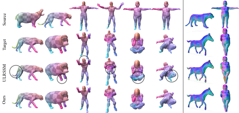
Figure 3: Qualitative Results on SMAL, DT4D-H, and TOPKIDS. Comparison of ULRSSM in the LBO basis and in the proposed hybrid basis. Hybrid functional maps yield higher-quality correspondences, particularly under topological noise. ULRSSM in the LBO basis frequently creates coarse mismatches such as incorrectly assigning appendages, whereas the elastic basis better represents these details. The first six columns show texture transfer. The last columns transfer normals making the less accurate alignment of creases in ULRSSM visible.

5 Experimental Results

This section provides a summary of the datasets used and our experimental setup. We refer to the appendix for a complete description of the datasets, splits, hyperparameters, and reformulation of method-specific losses in the HS-norm.

5.1 Datasets

We evaluate our method on several challenging benchmarks encompassing near-isometric (FAUST [7], SCAPE [2], SHREC [32], DeformingThings4D intra- [26]), non-isometric (SMAL [51], DeformingThings4D inter- [26]), and topologically noisy (TOPKIDS [28]) settings. We use the more challenging re-meshed versions as in previous works [15, 10].

5.2 Hybrid Basis in Different Frameworks

To understand the efficacy of the proposed hybrid basis in various methodological settings, we use it instead of the LBO basis in three different methods spanning supervised (GeomFMaps [13]), unsupervised (ULRSSM [10]), and axiomatic settings (Smooth Shells [16]). We re-run each of these three methods in their baseline LBO configuration for a fair comparison. Due to inherent variability, all experiments are conducted 5 times; we report the best results in alignment with standard practices. We additionally thoroughly analyze the different training scenarios and report the mean and std. dev. over all 5 runs on the SMAL dataset in Tab. 3. The total number of basis elements $k$ is kept fixed per method for all experiments; we replace only the highest-frequency LBO eigenfunctions with the elastic basis functions corresponding to the $l$ smallest eigenvalues. Quantitative experimental results can be found in Tab. 2 under the relevant section (supervised, unsupervised, axiomatic), where we compare to competitive methods in the same category. Qualitative results are shown in Fig. 3 and the supplementary.

GeomFMaps [13] originally proposed the addition of a Laplacian regularization term to the FMNet framework, which has proven effective at enforcing isometric characteristics of the map calculated from Eq. 2. We replace the LBO operator with the hybrid formulation, solving them separately as proposed in Thm. 4.3. For the elastic part of the functional map, we replace both the $E_{\text{data}}$ and $E_{\text{reg}}$ terms in the map optimization problem with our weighted variations. We also regularize the ground truth supervision loss $\mathcal{L}_{\text{gt}}$ = $(C-C_{\text{gt}})$ with the weighted HS-norm. We refine the hybrid functional map during inference to obtain dense point-to-point correspondences by performing a nearest-neighbor search in the hybrid vector space. Following the recommendations of the original authors [13], all final results in Tab. 2 are run at a spectral resolution of $k=30$, with $l=10$.

Results. We compare our results with those of GeomFMaps under the LBO basis and the supervised method FMNet [27]. Notably, the proposed hybrid basis outperforms LBO GeomFMaps in most settings, spanning near-isometric and non-isometric shape matching, where a particular benefit can be seen for SHREC’19 and SMAL, with a $2.3$ and $0.8$ improvement in mean geodesic error, respectively.

ULRSSM [10] has recently achieved SoTA performance in various challenging shape-matching settings. We evaluate our proposed hybrid basis when used in ULRSSM instead of the pure LBO functional basis. ULRSSM uses the functional map computation term described in Eq. 2, and hence, we proceed to split the optimization problem as described in Thm. 4.3 and adapt the elastic part with the proposed weighted formulation. The authors of ULRSSM additionally regularize the functional map $C$ to preserve bijectivity $\mathcal{L}_{\text{bij}}$, orthogonality $\mathcal{L}_{\text{orth}}$, and a loss coupling functional and point-to-point maps $\mathcal{L}_{\text{couple}}$ in a differentiable manner. For the elastic optimization, these are all reformulated in the HS-norm. We use the same overall spectral resolution as the authors $k=200$, with $l=60$ elastic basis functions [10]. This choice of basis ratio is discussed in the appendix.

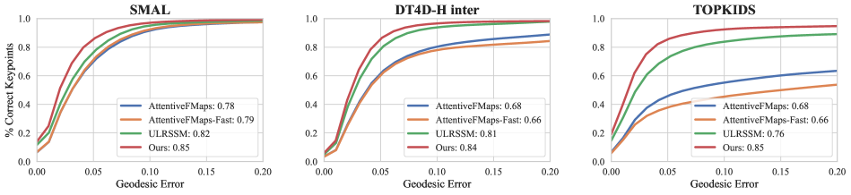
Figure 4: Percentage-Correct-Keypoint Plots depicting the geodesic error for state-of-the-art unsupervised methods on the datasets SMAL, DT4D-H inter, and TOPKIDS. We compare AttentiveFMaps, ULRSSM, and ULRSSM in the proposed hybrid basis.

Results. Using the hybrid basis instead of the LBO basis in ULRSSM results in notable performance improvements, even in near-isometric matching settings such as FAUST and SCAPE. Improvements are most significant in the non-isometric settings, including SMAL, where the hybrid basis outperforms LBO with a geodesic error of $0.6$ and inter-class DT4D-H with $0.7$. The most notable performance increase can be observed for TOPKIDS, where the hybrid basis yields a $45\%$ improvement in geodesic error.

Smooth Shells [16] remains one of the most strongly performing axiomatic methods for spectral shape matching. The method generates initial hypotheses for aligning a shape pair through a Markov-Chain Monte-Carlo (MCMC) step in a low-dimensional spectral basis ($k=20$). The algorithm then proceeds with an alternating optimization using both extrinsic and intrinsic information. Following the principle that Laplacian eigenfunctions capture coarse shape features well, we perform the MCMC initialization in the LBO basis. During the hierarchical matching step, we extend the product manifold with an additional dimension consisting of the elastic basis, incorporating the crease-aware functional map into the optimization. We use $300$ LBO and $l=200$ elastic basis functions, while the original implementation uses $k=500$ LBO basis functions. Results for DT4D-H are omitted due to excessive runtime.

Results. We observe that the performance with the proposed hybrid basis also leads to improved performance of Smooth Shells’ over pure LBO, particularly for non-isometric and topologically noisy settings. Notable improvements can be seen for the TOPKIDS and SMAL datasets, with a $3.3$ and $2.6$ improvement in mean geodesic error, respectively.

5.3 Ablation on Non-Orthogonality

As established in Sec. 4, losses using non-orthogonal basis sets require careful treatment to consider the non-uniform metric $M_{k}$ on the function spaces. This overhead could be circumvented by orthogonalizing the basis functions. However, while the span of the basis is preserved, we observe that orthogonalization affects the structure of the resulting functional maps. We conduct several experiments to better understand this adverse effect. Before solving the optimization problem in Eq. 4, we perform a Gram-Schmidt orthonormalization under the inner product induced by $M$, resulting in a set of orthogonal basis functions for each shape. We then construct a hybrid functional map without weighting any loss terms, treating the basis as if they were orthogonal. We additionally compare the effect of the weighted norms from Thm. 4.2 with a non-orthogonal elastic basis with no weighting. All experiments are conducted on ULRSSM in an unsupervised setting with $k=200$.

LBO	Elastic	Elastic Stabil.	Geo. error ($\times$100)
✗	✓	✗	$40.2\pm 0.80$
✗	✓	Orthog.	$5.75\pm 1.20$
✓	✗	✗	$5.15\pm 0.99$
✓	✓	✗	$4.37\pm 1.57$
✓	✓	Orthog.	$4.33\pm 0.56$
✓	✓	Weight. Norm	3.83 $\pm$ 0.74

Table 3: Ablation study observing the performance of the baseline ULRSSM [10], and ULRSSM hybridized under various conditions on the SMAL dataset. We observe the effect of two elastic stabilizations: orthogonalization (Orthog.) and optimization in the weighted norms (Weight. Norm) proposed in Sec. 4. Experiments are conducted 5 times; mean $\pm$ stdev. is reported.

Results. The results can be seen in Tab. 3. We observe that orthogonalization and omitting the weighting on the masses from Eq. 2 leads to inferior results. While the hybrid basis in ULRSSM improved the results, inter-run variability remains particularly high for the (un-weighted) elastic basis. Orthogonalization of the elastic basis functions in the hybrid functional maps has a stabilizing effect. The most pronounced performance gains are observed under proper weighting of $E(C)$ in Eq. 2 and network losses in Sec. 4.3.

5.4 Implementation

Implementations are carried out in Pytorch 2.1.0 with CUDA version 12.1, except for Smooth Shells, which is run in Matlab based on the implementation provided by the authors. Supervised and unsupervised methods are trained and evaluated on an NVIDIA A40. A complete list of hyperparameters for each of the methods used is provided in the appendix.

6 Limitations and Conclusion

This work explores the efficacy of combining basis functions from different operators for deformable shape correspondence. Our findings highlight the importance of accurately treating non-orthogonal basis functions to reflect the non-uniform metric on each shape. Imposing orthogonality on the basis functions shows improvement over naive adaptation but does not supplant proper mathematical adaptation of the optimization objectives. Additionally, the elastic basis functions underperform when used independently in a learned context; integrating it with low-frequency LBO basis functions significantly enhances spectral matching accuracy.

Solving the expanded $k^{2}\times k^{2}$ system from Thm. 4.2 leads to computational overhead; however, this is tractable for the elastic basis size of $l=60$. Performance gains in the expanded form justify this trade-off. Future research could approach partial shapes, point clouds, and real-world noisy data with non-orthogonal basis functions, as these are active areas of interest [4, 9, 21] and addressing robustness in these challenging settings with non-orthogonal basis functions.

Overall, the proposed hybrid functional mapping approach, leveraging both elastic and LBO eigenfunctions, exhibits notable performance in diverse settings, including isometric and non-isometric deformations and under topological noise. Our findings open new avenues for integrating various non-orthogonal basis functions into deep functional mapping frameworks, paving the way for further advances in spectral shape matching for challenging settings.

In the supplementary materials we first provide additional mathematical background in  Appendix A, along with complete derivations for Lemma 4.1, Thm. 4.2, and Thm. 4.3 in  Sec. A.2. We then detail datasets and splits used for evaluation in Sec. B.1, followed by further experimental details in Sec. B.2. Ablation studies concerning our design choices are provided in Appendix C. Finally, we present runtime analysis in Appendix D and additional qualitative results in Appendix E.

Appendix A Mathematical Background

We first provide definitions for the elastic and membrane energy construction for completeness. See [5, 20, 19] for a more detailed definition.

$$W_{\text{mem}} :\text{Membrane energy}$$

$$W_{\text{bend}} :\text{Bending energy}$$

$$\Gamma :\text{Change of metric under the deformation}$$

$$\bar{\mu},\bar{\lambda} :\text{Material constants}$$

$$\delta :\text{Thickness of the thin shell}$$

$$A :\text{Area of the triangle}$$

$$\alpha :\text{Dihedral angle in undeformed configuration}$$

$$\alpha^{\prime} :\text{Dihedral angle in deformed configuration}$$

The membrane and bending energies can then be constructed as follows:

$$W_{\text{mem}}[\mathbf{f}] =\int\delta\times A\times\bar{\mu}$$

$$\times\left(\text{tr}(\Gamma)+\bar{\lambda}\log\text{det}\Gamma-\bar{\mu}-\bar{\lambda}\right)$$

$$W_{\text{bend}}[\mathbf{f}] =\delta^{3}\sum A\times\left(\alpha-\alpha^{\prime}\right)^{2}$$

We can then solve the generalized eigenvalue problem for the Hessian at the identity to obtain the basis functions $\Psi$.

$$\text{Hess}\;\mathcal{W}_{S}[\text{Id}]v_{\lambda}=\lambda Mv_{\lambda}$$

For all our experiments, we use the same elastic energy hyperparameters as Hartwig et al. [19], including a bending weight of $10^{-2}$.

A.1 Problem setting

In the non-rigid correspondence literature, descriptors $D_{i}$ are commonly characterized as functions over the shapes $S_{i}$. In the discretized setting, many operations reduce to matrix-vector products. However, to derive the proper operations weighted by the non-uniform weight matrices $M$ in the regularization of the functional map, we utilize the more general hilbert space setting.

We assume that all functions on the spaces $\mathcal{F}(S_{i})$ are $L^{2}$ integrable:

$$L^{2}(\Omega):=\left\{f:\Omega\rightarrow\mathbb{R}\mid\int_{\Omega}|f(x)|^{2}\,dx<\infty\right\}$$

Then the inner product on each space $\mathcal{F}(S_{i})$ is given by $\langle\cdot,\cdot\rangle_{M}$ in the space induced by $M$:

$$\langle x,y\rangle_{M}=\int_{\Omega}x(t)y(t)\,dM(t)\stackrel{{\scriptstyle?}}{{=}}x^{\top}My$$ (6)

where in the last step we emphasize that the discretized operations reduce to matrix-vector multiplications in the finite-dimensional setting.

We use the definition of the Hilbert-Schmidt norm for a general operator $A$ on an (unweighted) Hilbert space [19, Sec 3.4]:

$$\|A\|_{HS}:=\sqrt{\text{tr}(A^{*}A)}$$ (7)

When $A:\mathcal{F}(S_{1})\to\mathcal{F}(S_{2})$ (the non-uniform weighted shape spaces), we have the following equivalence with the Frobenius norm [19]:

$$\|A\|^{2}_{HS}: =\text{tr}(M_{k,1}^{-1}A^{\top}M_{k,2}A)$$ (8)

$$=\text{tr}(\sqrt{M_{k,1}^{-1}}A^{\top}\sqrt{M_{k,2}}\sqrt{M_{k,2}}A\sqrt{M_{k,1}^{-1}})$$

$$=\left\|\sqrt{M_{k,2}}A\sqrt{M_{k,1}^{-1}}\right\|_{F}^{2}$$

A.2 Derivation of Eq. 2 for General Hilbert Spaces.

Proof of Lemma 4.1.

The data term can be interpreted as the difference of the descriptor functions $D_{1},D_{2}\in\mathcal{F}(S_{2})$ after $D_{1}$ was transferred to $\mathcal{F}(S_{2})$ via the functional map $C$. We denote the first k eigenfunctions by $\Psi_{k,i}$ and the coefficients of $D_{i}$ projected into the basis spanned by these eigenfunctions by $D_{\Psi_{i}}:=\Psi_{k,i}^{\dagger}D_{i}$. We then have the following:

$$\|CD_{\Psi_{1}}-D_{\Psi_{2}}\|_{M_{k,2}}$$

$$=\ \sqrt{\langle CD_{\Psi_{1}}-D_{\Psi_{2}},CD_{\Psi_{1}}-D_{\Psi_{2}}\rangle_{M_{k,2}}}$$

$$= \sqrt{\text{tr}((CD_{\Psi_{1}}-D_{\Psi_{2}})^{\top}M_{k,2}(CD_{\Psi_{1}}-D_{\Psi_{2}}))}$$

where we use the definition of the inner product Eq. 6, the cyclicity of the trace. The identity then follows by splitting $M_{k,2}=\sqrt{M_{k,2}}\sqrt{M_{k,2}}$ and applying the definition of the Frobenius norm again, and using that $M_{k,2}$ is symmetric.

∎

As previously established [13], the energy in Eq. 2 can be solved for $C$ in closed form by solving $k$ different $k\times k$ linear systems (for each row of $C$). In our case, the mass matrices $M$ prohibit this, requiring an expansion to a $k^{2}\times k^{2}$ system. This expansion is detailed below.

Proof of  Thm. 4.2.

Let $S_{1}$ and $S_{2}$ be Hilbert spaces defined on two shapes associated with mass matrices $M_{k,1}$ and $M_{k,2}$, respectively, which induce the inner product on each space. Let $\Lambda_{1}$ and $\Lambda_{2}$ be the diagonal matrices of Laplacian eigenvalues on $S_{1}$ and $S_{2}$, and let $C$: $\mathcal{F}(S_{1})\to\mathcal{F}(S_{2})$ be a linear map between the function spaces. The weighted Laplacian commutativity regularization term can be expressed using the Hilbert-Schmidt norm as follows:

$$||(C\Lambda_{1} -\Lambda_{2}C)||_{HS}^{2}$$

$$=\text{tr}(M_{k,1}^{-1}(C\Lambda_{1}-\Lambda_{2}C)^{\top}M_{k,2}(C\Lambda_{1}-\Lambda_{2}C))$$

$$=\left\|\sqrt{M_{k,2}}\left(C\Lambda_{1}-\Lambda_{2}C\right)\sqrt{M_{k,1}^{-1}}\right\|_{\text{F}}$$

$$=\left\|\sqrt{M_{k,2}}C\Lambda_{1}\sqrt{M_{k,1}^{-1}}-\sqrt{M_{k,2}}\Lambda_{2}C\sqrt{M_{k,1}^{-1}}\right\|_{\text{F}}$$

where we apply the definition of the HS-norm Eq. 8, the definition of the Frobenius norm, and multiply out the terms.

As previously established [13, 40], the Laplacian commutivity operator can be represented as an element-wise product between a penalty mask matrix $M_{LB}$ and the map $C$, where $M_{\text{LB}}(i,j)=\Lambda_{1}(i)^{2}-\Lambda_{2}(j)^{2}$ and $\Lambda_{1}$, $\Lambda_{2}$ are vectors of the eigenvalues of $\Delta_{1}$ and $\Delta_{2}$ respectively. Note that this formulation can be used with either the Laplacian or more frequently used Resolvant regularization terms.

Now, we can use the definition of the Kronecker product

$$\text{vec}(ABC)=\left(C^{\top}\otimes A\right)\text{vec}(B)$$ (9)

to expand and rearrange this into the form $||\zeta x||_{F}$ for a matrix $\zeta$ and vector $x:=\text{vec}(C)$:

$$\lVert\sqrt{M_{k,2}} \left(C\Lambda_{1}-\Lambda_{2}C\right)\sqrt{M_{k,1}}\rVert_{\text{F}}^{2}$$

$$=\ \lVert((\Lambda_{1}\sqrt{M_{k,1}^{-1}})\otimes\sqrt{M_{k,2}}\ -$$

$$\sqrt{M_{k,1}^{-1}}\otimes(\sqrt{M_{k,2}}\Lambda_{2}))\text{vec}(C)\rVert_{F}^{2}$$

∎

A.3 Solving the Combined Optimization Problem

To solve $E(C)$ for a vectorized functional map $C$, $E_{\text{data}}$ must be expanded similarly. Using Eq. 9 we have:

$${\|\sqrt{M_{k,2}}(CD_{\Psi_{1}}-D_{\Psi_{2}})\|}_{F}$$

$$={\|vec(\sqrt{M_{k,2}}CD_{\Psi_{1}})-vec(\sqrt{M_{k,2}}D_{\Psi_{2}}))\|}_{2}$$

$$={\|((\sqrt{M_{k,2}}D_{\Psi_{1}})^{\top}\otimes I)vec(C)-vec(\sqrt{M_{k,2}}D_{\Psi_{2}})\rVert}_{2}$$

Where we use the fact that the Frobenius norm of a matrix is just the $L_{2}$ norm of its stacked column vectors and the definition of the Kroeneker product. Combining the expanded forms of $E_{\text{data}}$ and $E_{\text{reg}}$ and observing the first variation of $E(C)$ yields a $k^{2}\times k^{2}$ linear system which can be solved for $C$:

$$(A^{\top}A+\lambda\zeta^{\top}\zeta)vec(C)-A^{\top}vec(B)=0$$

Here, we made the following substitutions for readability:

$$A=(\sqrt{M_{k,2}}D_{\Psi_{1}})^{\top}\otimes I$$

$$B=\sqrt{M_{k,2}}D_{\Psi_{2}}$$

$$\zeta=(\Lambda_{1}\sqrt{M_{k,1}^{-1}})\otimes\sqrt{M_{k,2}}-\sqrt{M_{k,1}^{-1}}\otimes(\sqrt{M_{k,2}}\Lambda_{2})$$

A.4 Optimization Block Matrix Formulation

Proof of  Thm. 4.3.

The block matrix representation of the functional map $C$ in the hybrid vector space is given by

$$C=\begin{pmatrix}C^{11}&C^{12}\\ C^{21}&C^{22}\end{pmatrix},$$ (10)

where $C^{11}$ and $C^{22}$ represent the functional maps within the same basis types, and $C^{12}$ and $C^{21}$ represent the functional maps between different basis types. Let

$$D_{\xi_{i}}:=\begin{bmatrix}D_{\Phi_{i}}\\ D_{\Psi_{i}}\end{bmatrix}$$

denote the descriptors in the combined vector space. Here we use an LBO basis of size $k-l$ and an elastic basis of size $l$. Furthermore, we let $\Sigma_{i}:=diag(\lambda_{1},...\lambda_{k-l},\theta_{1},...,\theta_{l})$ the diagonal matrix of combined eigenvalues from $\Delta_{i}$ and $\text{Hess}\mathcal{W}_{S}[\text{Id}]$, respectively. Then, both the data and regularization terms in Eq. 2 can be expanded:

$$E(C)=\|CD_{\xi_{1}}-D_{\xi_{2}}\|_{F}^{2}+\lambda\|C\Lambda_{1}-\Lambda_{2}C\|_{F}^{2}.$$

We can express the data term in the block matrix format:

$$\begin{split}\|CD_{\xi_{1}}-D_{\xi_{2}}\|_{F}^{2}=&\left\|\begin{pmatrix}C^{11}&C^{12}\\ C^{21}&C^{22}\end{pmatrix}\begin{bmatrix}D_{\Phi_{1}}\\ D_{\Psi_{1}}\end{bmatrix}-\begin{bmatrix}D_{\Phi_{2}}\\ D_{\Psi_{2}}\end{bmatrix}\right\|_{F}^{2}\end{split}$$

Expanding this and separating the terms associated with the LBO and elastic bases gives us the following:

$$\left\lVert\begin{bmatrix}C^{11}D_{\Phi_{1}}+C^{12}D_{\Psi_{1}}-D_{\Phi_{2}}\\ C^{21}D_{\Phi_{1}}+C^{22}D_{\Psi_{1}}-D_{\Psi_{2}}\end{bmatrix}\right\rVert_{F}$$

Due to the additivity of the Frobenius norm, the two terms can be minimized separately. However, note that the functional maps $C^{11}$ and $C^{22}$ depend on the off-diagonal blocks $C^{12}$ and $C^{21}$, respectively. This problem can thus be separated if and only if the off-diagonal blocks $C^{12}$ and $C^{21}$ are $0$, ensuring that there are no intra-basis matchings during the optimization.

To see that a similar condition holds for the regularization term, we observe that it can be written as an element-wise product of the eigenvalues associated with the respective basis and the functional map [13, 40]:

$$E_{\text{reg}}(C) =||C\ \Sigma_{1}-\Sigma_{2}\ C||^{2}$$

$$=\sum_{i,j}M_{ij}C_{ij}^{2}$$

where $M_{ij}=(\Lambda_{2}(i)-\Lambda_{1}(j))^{2}$. We note that for the block matrix representation, only the off-diagonal entries $C^{12}$ and $C^{21}$ correspond to eigenvalues $\Lambda_{i}$ and $\Lambda_{j}$ from different respective basis functions. Thus, if the off-diagonal functional maps are $\mathbf{0}$, these cross-basis regularization terms do not impact the optimization. Hence, the regularization term $E_{\text{reg}}$ can be similarly separated. This argument holds for both the eigenvalue regularization used in GeomFMaps, [13] as well as resolvant regularization [40] as both formulations can be reduced to an element-wise multiplication.

Now, the optimization problem decouples into two separate problems, one for each basis type. These can be solved independently to obtain the optimal functional maps $C^{*}_{11}$ and $C^{*}_{22}$ within the LBO and elastic bases, respectively.

$$C^{11}_{*} =\arg\min_{C^{11}}E_{\text{LB}}(C^{11})$$

$$C^{22}_{*} =\arg\min_{C^{22}}E_{\text{Elas}}(C^{22})$$

∎

Appendix B Implementation Details

B.1 Datasets

We evaluate our method across near-isometric, non-isometric, and topologically noisy settings. Splits are chosen based on standard practices in the recent literature [15, 10].

Near-isometric:

The FAUST, SCAPE, and SHREC’19 datasets represent near-isometric deformations of humans, with 100, 71, and 44 subjects, respectively. We follow the standard train/test splits for FAUST and SCAPE: : 80/20 for FAUST and 51/20 for SCAPE. Evaluation of our method on SHREC’19 is conducted with a model trained on a combination of FAUST and SCAPE inline with recent methods [25, 15, 10]. We use the more challenging re-meshed versions as in recent works.

Non-isometric:

The SMAL dataset features non-isometric deformations between 49 four-legged animal shapes from eight classes. The dataset is split 5/3 by animal category as in Donati et al. [15], resulting in a train/test split of 29/20 shapes. We further evaluate the large animation dataset DeformingThings4D (DT4D-H) [26], using the same inter- and intra-category splits as Donati et al. [15].

Topological Noise:

The TOPKIDS dataset [28] consists of shapes of children featuring significant topological variations and poses a significant challenge for unsupervised functional map-based works. Considering its limited size of 26 shapes, we restrict our comparisons to axiomatic and unsupervised methods and use shape 0 as a reference for matching with the other 25 shapes, following recent methods [16, 15, 10].

B.2 Experimental Details

In this section we provide additional details regarding the evaluation of our proposed hybrid basis from Sec. 5, including the axiomatic, supervised, and unsupervised settings. Unless otherwise mentioned, implementations and parameters are left unaltered for the hybrid adaptation.

We first provide general details regarding learning and then the individual adaptations for each method. Learned methods (GeomFMaps [13] and ULRSSM [10]) are trained with PyTorch, using DiffusionNet as the feature extractor and WKS descriptors as input features, except for the SMAL dataset where we use XYZ signal with augmented random rotation as in recent methods [25, 10]. The dimension of the output features is fixed at 256 for all experiments.

For both learned methods, we propose the following linear annealing scheme for learning in a hybrid basis, as mentioned in Sec. 4.3.

$$\mathcal{L}_{\text{total}}=\alpha\mathcal{L}_{\text{LB}}+ \mu\ \beta\ \mathcal{L}_{\text{Elas}}$$

$$\alpha=\frac{1}{2}\cdot\frac{k^{2}}{(k-l)^{2}}\qquad \beta=\frac{1}{2}\cdot\frac{k^{2}}{l^{2}}$$

Where $k$ is the total number of basis functions, and $l$ is the number of elastic basis functions. The parameters $\alpha$ and $\beta$ ensure the losses are normalized w.r.t. the number of entries in the functional map similar to the approach of Li et al. [25]. We increase $\mu$ over the first 2000 iterations so that the less-robust elastic basis functions do not adversely affect feature initialization.

Hybrid GeomFMaps.

We use 30 total eigenfunctions as in the original work. For the hybrid adaptation, 20 LBO and 10 Elastic basis functions are used as the spectral resolution. To compute the functional map, we use the standard regularized functional map solver and set $\lambda=1\times 10^{-3}$ as in the original work [13]. For the hybrid adaptation, we empirically set $\lambda=5\times 10^{-4}$ for the elastic solver.

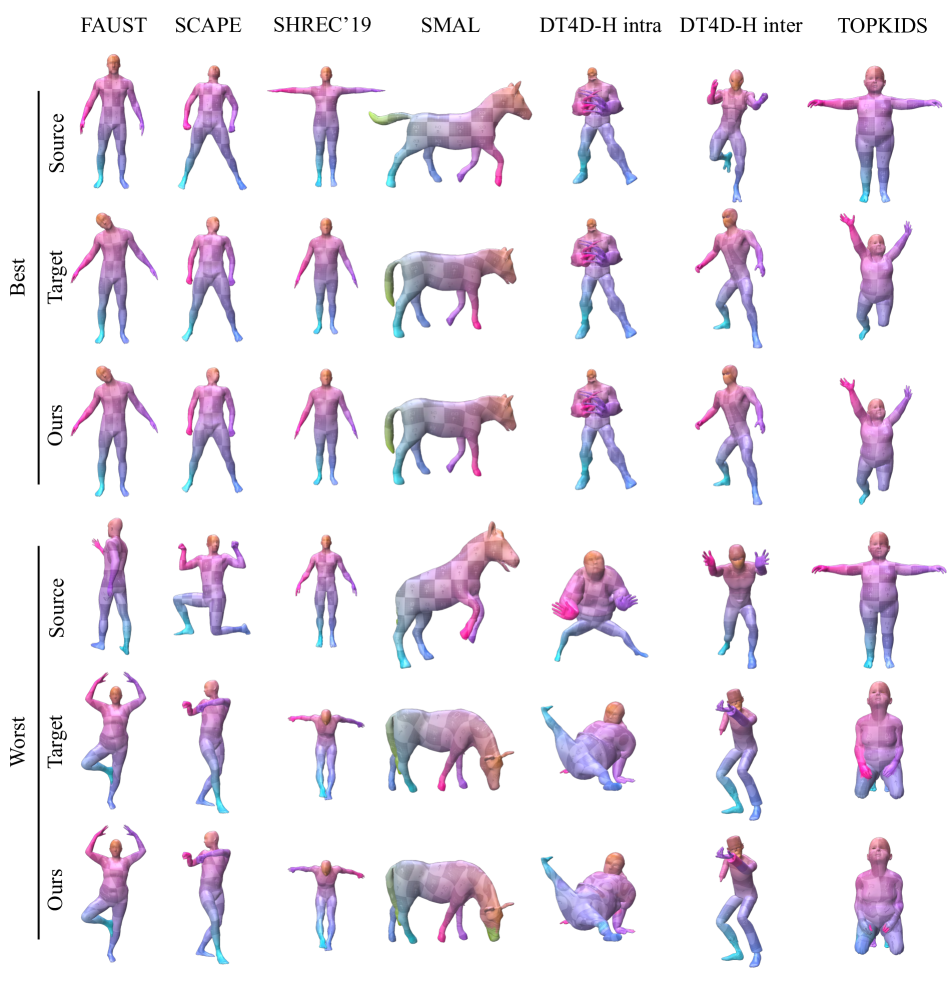
Figure 5: Additional qualitative results for the best and worst predictions of ULRSSM in the proposed hybrid basis (our method).

GeomFMaps is supervised using a functional map constructed from the ground-truth correspondences. We thus adapt the elastic loss as follows (note here C refers to $\mathcal{F}(S_{1})\to\mathcal{F}(S_{2})$ as the original work [13]):

$$\mathcal{L}_{\text{Elas}}=\left\|C-C_{\text{gt}}\right\|_{\text{HS}}^{2}=\|\sqrt{M_{k,2}}(C-C_{\text{gt}})\sqrt{M^{-1}_{k,1}}\|_{F}^{2}$$

Hybrid ULRSSM.

The ULRSSM baseline [10] uses a spectral resolution of $k=200$. We keep the total number of basis functions fixed at $k=200$, using $(k-l)=140$ LBO and $l=60$ Elastic eigenfunctions.

For the functional map computation, we use the Resolvent regularized functional map solver [40] for LB map block setting $\lambda=100$ as in the original work. Our adapted variant is weighted empirically with $\lambda=50$ for the elastic block. ULRSSM regularizes the functional map obtained from Eq. 2 with 3 losses: bijectivity, orthogonality, and a coupling loss with the point-to-point map. The loss for the LBO functional map block $\mathcal{L}_{\text{LB}}$ is kept the same as the baseline method while we adapt the bijectivity, orthogonality, and coupling terms for the elastic block in the HS-norm.

In the following, $C$ represents the block-functional map’s elastic part for clarity. Without loss of generality we let $C_{12}:\mathcal{F}(S_{1})\to\mathcal{F}(S_{2})$. While the bijectivity loss is left unchanged, we adapt the $\mathcal{L}_{\text{orth}}$ term using the adjoint $C^{*}$ as follows, similar to Hartwig et al. in their adapted ZoomOut [19]:

$$\mathcal{L}_{\text{orth}} =\left\|C_{12}^{*}C_{12}-I\right\|_{\text{HS}}^{2}+\left\|C_{21}^{*}C_{21}-I\right\|_{\text{HS}}^{2}$$

$$=\left\|C_{21}^{*}C_{21}-I\right\|_{F}^{2}+\left\|C_{12}^{*}C_{12}-I\right\|_{F}^{2}$$

We note that concerning the respective bijectivity and orthogonality losses, the operators $C_{12}C_{21}-I$ and $C_{21}^{*}C_{21}-I$ map to and from the same function space, thus the HS-norm is equivalent to the standard Frobenius norm and requires no non-uniform weighting.

The $\mathcal{L}_{\text{couple}}$ term is given by:

$$\mathcal{L}_{\text{couple}} =\left\|C_{12}-\Psi_{2}^{\dagger}\Pi_{21}\Psi_{1}\right\|_{\text{HS}}^{2}+\left\|C_{21}-\Psi_{1}^{\dagger}\Pi_{12}\Psi_{2}\right\|_{\text{HS}}^{2}$$

$$=\left\|\sqrt{M_{k,2}}(C_{12}-\Psi_{2}^{\dagger}\Pi_{21}\Psi_{1})\sqrt{M^{-1}_{k,1}}\right\|_{F}^{2}$$

$$+\left\|\sqrt{M_{k,1}}(C_{21}-\Psi_{1}^{\dagger}\Pi_{12}\Psi_{2})\sqrt{M^{-1}_{k,2}}\right\|_{F}^{2}$$

For the definition of the point-to-point maps $\Pi_{21}$ and $\Pi_{12}$ we refer readers to the original method [10].

Empirically, we set $\lambda_{\text{bij}}=\lambda_{\text{orth}}=\lambda_{\text{couple}}=1.0$ for the LB part following the original work. We keep these parameters the same for the elastic block except setting $\lambda_{\text{orth}}=0.0$ as we observed the orthogonality constraint adversely affects the method’s performance.

Hybrid SmoothShells.

To demonstrate how the proposed hybrid basis can be used in an axiomatic method, we adapt the method SmoothShells [16] with the minimally needed changes.

The initialization of SmoothShells consists of a low-frequency MCMC alignment. We keep this step as-is and do not replace the LBO smoothing with the hybrid eigenfunctions because the elastic eigenfunctions cannot achieve low-frequency smoothing by design. We fix the random seed and re-run the baseline Smooth Shells and the hybrid version with the same MCMC initialization to rule out noise.

The main idea of Smooth Shells [16] is to achieve a coarse-to-fine alignment by iteratively adding higher-frequency LBO eigenfunctions to the intrinsic-extrinsic embedding. Instead of only adding LBO eigenfunctions in a new iteration, we add a ratio of LBO and elastic eigenfunctions. As in the other adaptations, we keep the total number of basis functions $k=500$ fixed. We then empirically replace the highest $l=200$ LBO eigenfunctions with elastic eigenfunctions, modifying the product embedding to be:

$$\mathbf{X}_{k} :=\left(\Phi_{1,k},\Psi_{1,k},X_{k},\mathbf{n}_{k}^{S_{1}}\right)\in\mathbb{R}^{n_{1}\times(k+6)}$$

$$\mathbf{Y}_{k} :=\left(\Phi_{2,k},\Psi_{2,k},Y_{k},\mathbf{n}_{k}^{S_{2}}\right)\in\mathbb{R}^{n_{2}\times(k+6)}$$

where we use our notation of the LBO and elastic basis functions. $\mathbf{X}_{k},\mathbf{Y}_{k}$ are the product embeddings for shape $S_{1}$ and $S_{2}$ with $X_{k},Y_{k}$ the respective smoothed cartesian coordinates, and $\mathbf{n}_{k}$ the outer normals on each shape. The rest of the optimization follows directly from [16].

Appendix C Further Ablation Studies

In this section, we present the results of several ablation studies, focusing on key design choices: the hybridization of the basis, our optimization strategies, and experimental results concerning separating the optimization problems from Thm. 4.3.

C.1 Basis Ratio

To validate the effectiveness of our choice of hybridizing between the LB (Laplace-Beltrami) and Elastic eigenfunctions, we conduct extensive ablation experiments showcasing the performance of different ratios of hybridized basis.

In all these experiments, we again fix the total number of basis functions used as $k$ while replacing the $l$ highest frequency LB basis with the Elastic eigenfunctions corresponding to the $l$ smallest eigenvalues. This follows the intuition that the low-frequency LB basis functions enable coarse shape alignment while failing to capture fine details, while optimizing in the hybrid basis enables alignment to thin structures and high curvature details better than in the pure LBO basis. We conduct two ablations to demonstrate such a choice; both experiments were carried out on the SMAL dataset for its challenging non-isometry and practical relevance as a stress test.

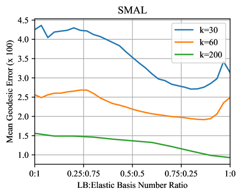
Figure 6: Ground truth reconstruction using a varying ratio of LBO and elastic eigenfunctions, with different total numbers of basis functions k.

Ground-Truth Reconstruction

For ground-truth reconstruction, a ground-truth point-to-point map is projected into the spectral domain. Subsequently, a nearest neighbor search can be used to reconstruct the point correspondences, where a discrepancy with the ground-truth point-to-point map is measured. This simple experimental scenario enables a convenient way to measure the expressiveness of a functional map between two basis sets; however, it cannot encompass all characteristics of a functional map. In Fig. 6, we consider the hybrid basis composed with a varying ratio of LBO and elastic basis functions and a different number of total basis functions: $k=30,60$, and $200$. We measure the mean geodesic error between the ground-truth point-to-point map and the reconstruction from the hybrid functional maps.

Results. The hybridized basis can notably better represent the ground truth for $k=30$ and $60$. We observe an optimum of around 80% LBO and 20% elastic eigenfunctions. This phenomenon diminishes at $k=200$, suggesting the LB basis functions can indeed represent fine details with a sufficiently high number of basis functions. However, ground-truth reconstruction does not necessarily represent the setting where features are learned through backpropagation of the functional map loss. Our experiments indicate that learned pipelines cannot leverage the high-frequency LBO eigenfunctions to represent fine extrinsic details as effectively as the elastic basis functions, even with a large total number of basis functions. We, therefore, conduct a similar ablation in the learned setting.

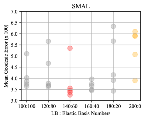
Figure 7: Hybrid ULRSSM is evaluated on SMAL using a varying ratio of LBO and elastic eigenfunctions. Our basis ratio can be observed in red, with the baseline pure LBO implementation in yellow.

Learned Setting.

In Fig. 7, we consider the hybrid ULRSSM method with a fixing total basis number of $k=200$ under different hybrid basis ratios with a step size of $20$. Due to the polynomially (see  Appendix D) increasing computations for the $k^{2}\times k^{2}$ system, we limit the number of elastic basis functions to less than $100$ (GT-reconstruction also indicates inferior performance in this regime). We run each experiment 5 times to eliminate inherent noise and report all results.

Results. Here, we observe that a ratio of around 140:60 is optimal; the hybridized basis (red) shows consistent performance improvements over the baseline (orange) and other basis ratios.

C.2 Optimization Strategies

Training a reliable shape correspondence estimation pipeline through hybrid functional maps involves several key modeling decisions. Both the linearly increasing scheduler for the elastic loss during training and normalizing factors for both Laplace-Beltrami (LB) and elastic losses play a large role in the obtained performance increases.

As mentioned in Sec. 4, we observed the elastic basis functions are not robust to uninitialized features. Easing in the elastic loss after feature initialization in the LBO basis mitigates convergence to undesirable local minima. Furthermore, the loss of each component in the hybrid functional map is normalized according to the number of matrix elements for this component, an important hyperparameter to balance the two blocks. During the ablation studies presented in Fig. 8, we selectively eliminate each one of these factors from our model and measure the mean geodesic error. We further demonstrate that fine-tuning from a pre-trained LBO checkpoint is ineffective, likely converging to local minima.

Results. The results in  Fig. 8 show that each component is indeed important for our final model. Fine-tuning from a checkpoint or training without normalization yields inferior results. Furthermore, except for a single outlier, our approach converges to a significantly lower minimum than learning without the linear-annealing strategy.

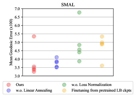
Figure 8: Ablation study of optimization strategies using Hybrid ULRSSM on SMAL. Five random runs are shown for each training setting.

C.3 Block Matrix Formulation

As detailed in Thm. 4.3, setting the off-diagonal blocks of the hybrid functional map to $\mathbf{0}$ is equivalent to solving the optimization problems separately. Here, we show this is both important computationally and in terms of regularization.

To demonstrate its regularization effect, we conduct an experiment in ULRSSM on the FAUST dataset comparing solving a hybrid functional map with our proposed method against naively via a single solve. This experiment is conducted with the orthogonalized elastic basis as a proof-of-concept, as solving a full-dimensional ($k=200$) hybrid functional map from the $k^{2}\times k^{2}$ system would be prohibitively expensive.

Results. The results of this ablation are depicted in Fig. 9. We observe that solving the two maps separately yields notably faster convergence compared to the naive approach with a marginal performance advantage. This suggests that a block-diagonal functional map is desirable; restricting inter-basis matches leads to faster convergence. Separately solving the optimization problems can be interpreted as a strong regularization of the off-diagonal blocks, reducing the search space.

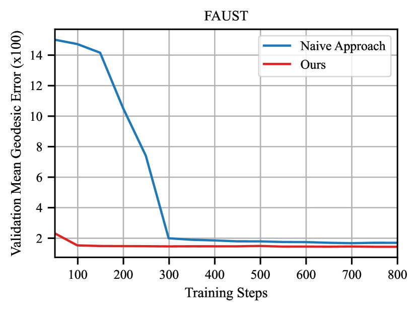
Figure 9: Ablation study concerning separate optimization of the block matrix on FAUST with Hybrid ULRSSM. The y-axis depicts validation error, while the x-axis shows training steps. Separating the optimization problems primarily leads to faster convergence.

Method	Runtime
ULRSSM	610.70 $\pm$ 45.20 ms
Hybrid ULRSSM	623.19 $\pm$ 32.03 ms

Table 4: Comparison of per-iteration runtime on SMAL over 100 training iterations (mean $\pm$ st. dev).

Appendix D Runtime Analysis

We provide our runtime analysis for the Hybrid ULRSSM method in SMAL dataset under Table 4. Results are obtained on an NVIDIA A40. Our hybrid adaptation incurs minimal runtime overhead while yielding significant performance gains despite needing to solve an expanded $k^{2}\times k^{2}$ system. This can be explained by analyzing the complexity. Assuming the complexity of solving a linear system for an $k\times k$ matrix is $\mathcal{O}(k^{3})$, solving the combined optimization problem costs $\mathcal{O}(k^{4})$ flops (since we solve $k$ separate $k\times k$ systems. Solving the separate optimization problem costs $\mathcal{O}((k-l)^{4}+l^{6})$ flops, which for the total basis number $k=200$ and elastic eigenfunctions $l=60$ is only one order of magnitude larger.

Appendix E Additional Qualitative Results

We provide additional qualitative results in Fig. 5 on each dataset. We evaluate and visualize the best and worst predictions of ULRSSM in the proposed hybrid basis.

References

- Andreux et al. [2014] M. Andreux, E. Rodolà, M. Aubry, and D. Cremers. Anisotropic laplace-beltrami operators for shape analysis. In Proc. European Conference on Computer Vision Workshops (ECCV - NORDIA), Zurich, Switzerland, 2014.
- Anguelov et al. [2005] Dragomir Anguelov, Praveen Srinivasan, Daphne Koller, Sebastian Thrun, Jim Rodgers, and James Davis. SCAPE: shape completion and animation of people. In ACM SIGGRAPH 2005 Papers, pages 408–416, New York, NY, USA, 2005. Association for Computing Machinery.
- Arun et al. [1987] Somani Arun, Thomas S. Huang, and Steven D. Blostein. Least-square fitting of two 3-d point sets. IEEE Pattern Analysis and Machine Intelligence, 9(5), 1987.
- Attaiki et al. [2021] Souhaib Attaiki, Gautam Pai, and Maks Ovsjanikov. DPFM: Deep Partial Functional Maps. In 2021 International Conference on 3D Vision (3DV), pages 175–185, 2021. ISSN: 2475-7888.
- Aubry et al. [2011] Mathieu Aubry, Ulrich Schlickewei, and Daniel Cremers. The wave kernel signature: A quantum mechanical approach to shape analysis. In 2011 IEEE International Conference on Computer Vision Workshops (ICCV Workshops), pages 1626–1633, 2011.
- Bastian et al. [2023] Lennart Bastian, Alexander Baumann, Emily Hoppe, Vincent Bürgin, Ha Young Kim, Mahdi Saleh, Benjamin Busam, and Nassir Navab. S3M: Scalable Statistical Shape Modeling Through Unsupervised Correspondences. In Medical Image Computing and Computer Assisted Intervention – MICCAI 2023, pages 459–469, Cham, 2023. Springer Nature Switzerland.
- Bogo et al. [2014] Federica Bogo, Javier Romero, Matthew Loper, and Michael J. Black. FAUST: Dataset and Evaluation for 3D Mesh Registration. In 2014 IEEE Conference on Computer Vision and Pattern Recognition, pages 3794–3801, Columbus, OH, USA, 2014. IEEE.
- Cao and Bernard [2022] Dongliang Cao and Florian Bernard. Unsupervised Deep Multi-shape Matching. In Computer Vision – ECCV 2022, pages 55–71, Cham, 2022. Springer Nature Switzerland.
- Cao and Bernard [2023] Dongliang Cao and Florian Bernard. Self-Supervised Learning for Multimodal Non-Rigid 3D Shape Matching, 2023. arXiv:2303.10971 [cs].
- Cao et al. [2023] Dongliang Cao, Paul Roetzer, and Florian Bernard. Unsupervised Learning of Robust Spectral Shape Matching, 2023. arXiv:2304.14419 [cs].
- Colombo et al. [2022] Michele Colombo, Giacomo Boracchi, and Simone Melzi. Pc-gau: Pca basis of scattered gaussians for shape matching via functional maps. In Smart Tools and Applications in Graphics (STAG), 2022.
- Deng et al. [2022] Bailin Deng, Yuxin Yao, Roberto M. Dyke, and Juyong Zhang. A Survey of Non-Rigid 3D Registration. Computer Graphics Forum, 41(2):559–589, 2022. _eprint: https://onlinelibrary.wiley.com/doi/pdf/10.1111/cgf.14502.
- Donati et al. [2020] Nicolas Donati, Abhishek Sharma, and Maks Ovsjanikov. Deep Geometric Functional Maps: Robust Feature Learning for Shape Correspondence. In 2020 IEEE/CVF Conference on Computer Vision and Pattern Recognition (CVPR), pages 8589–8598, Seattle, WA, USA, 2020. IEEE.
- Donati et al. [2021] Nicolas Donati, Etienne Corman, Simone Melzi, and Maks Ovsjanikov. Complex Functional Maps : a Conformal Link Between Tangent Bundles, 2021. Number: arXiv:2112.09546 arXiv:2112.09546 [cs, math].
- Donati et al. [2022] Nicolas Donati, Etienne Corman, and Maks Ovsjanikov. Deep Orientation-Aware Functional Maps: Tackling Symmetry Issues in Shape Matching, 2022. Number: arXiv:2204.13453 arXiv:2204.13453 [cs, math, stat].
- Eisenberger et al. [2020a] Marvin Eisenberger, Zorah Lahner, and Daniel Cremers. Smooth Shells: Multi-Scale Shape Registration With Functional Maps. In 2020 IEEE/CVF Conference on Computer Vision and Pattern Recognition (CVPR), pages 12262–12271, Seattle, WA, USA, 2020a. IEEE.
- Eisenberger et al. [2020b] Marvin Eisenberger, Aysim Toker, Laura Leal-Taixé, and Daniel Cremers. Deep Shells: Unsupervised Shape Correspondence with Optimal Transport. arXiv:2010.15261 [cs], 2020b. arXiv: 2010.15261.
- Halimi et al. [2019] Oshri Halimi, Or Litany, Emanuele Rodola Rodola, Alex M. Bronstein, and Ron Kimmel. Unsupervised Learning of Dense Shape Correspondence. In 2019 IEEE/CVF Conference on Computer Vision and Pattern Recognition (CVPR), pages 4365–4374, Long Beach, CA, USA, 2019. IEEE.
- Hartwig et al. [2023] Florine Hartwig, Josua Sassen, Omri Azencot, Martin Rumpf, and Mirela Ben-Chen. An Elastic Basis for Spectral Shape Correspondence. In Special Interest Group on Computer Graphics and Interactive Techniques Conference Conference Proceedings, pages 1–11, Los Angeles CA USA, 2023. ACM.
- Heeren et al. [2014] B. Heeren, M. Rumpf, P. Schröder, M. Wardetzky, and B. Wirth. Exploring the Geometry of the Space of Shells. Computer Graphics Forum, 33(5):247–256, 2014. _eprint: https://onlinelibrary.wiley.com/doi/pdf/10.1111/cgf.12450.
- Huang et al. [2022] Jiahui Huang, Tolga Birdal, Zan Gojcic, Leonidas J. Guibas, and Shi-Min Hu. Multiway Non-rigid Point Cloud Registration via Learned Functional Map Synchronization. IEEE Transactions on Pattern Analysis and Machine Intelligence, pages 1–1, 2022. arXiv: 2111.12878.
- Huang et al. [2019] Ruqi Huang, Panos Achlioptas, Leonidas Guibas, and Maks Ovsjanikov. Limit Shapes – A Tool for Understanding Shape Differences and Variability in 3D Model Collections. Computer Graphics Forum, 38(5):187–202, 2019.
- Kezurer et al. [2015] S. Kezurer, Z. Kovalsky, R. Basri, and Y. Lipman. Tight relaxation of quadratic matching. Computer Graphics Forum (CGF), 34, 2015.
- Li et al. [2008] Hao Li, Robert W. Sumner, and Mark Pauly. Global correspondence optimization for non-rigid registration of depth scans. Computer Graphics Forum, Symposium on Geometry Processing, 27(5), 2008.
- Li et al. [2022] Lei Li, Nicolas Donati, and Maks Ovsjanikov. Learning Multi-resolution Functional Maps with Spectral Attention for Robust Shape Matching, 2022. arXiv:2210.06373 [cs].
- Li et al. [2021] Yang Li, Hikari Takehara, Takafumi Taketomi, Bo Zheng, and Matthias Nießner. 4DComplete: Non-Rigid Motion Estimation Beyond the Observable Surface. pages 12706–12716, 2021.
- Litany et al. [2017] Or Litany, Tal Remez, Emanuele Rodolà, Alex M. Bronstein, and Michael M. Bronstein. Deep Functional Maps: Structured Prediction for Dense Shape Correspondence. arXiv:1704.08686 [cs], 2017. arXiv: 1704.08686.
- Lähner et al. [2016] Z Lähner, E Rodolà, M M Bronstein, D Cremers, O Burghard, L Cosmo, A Dieckmann, R Klein, and Y Sahilliog. SHREC’16: Matching of Deformable Shapes with Topological Noise. Eurographics Workshop on 3D Object Retrieval, EG 3DOR, pages 55–60, 2016.
- Magnet et al. [2023] Robin Magnet, Kevin Bloch, Maxime Taverne, Simone Melzi, Maya Geoffroy, Roman H. Khonsari, and Maks Ovsjanikov. Assessing craniofacial growth and form without landmarks: A new automatic approach based on spectral methods. Journal of Morphology, 284(8):e21609, 2023. _eprint: https://onlinelibrary.wiley.com/doi/pdf/10.1002/jmor.21609.
- Marin et al. [2020] Riccardo Marin, Marie-Julie Rakotosaona, Simone Melzi, and Maks Ovsjanikov. Correspondence learning via linearly-invariant embedding. In Advances in Neural Information Processing Systems, pages 1608–1620. Curran Associates, Inc., 2020.
- Melzi et al. [2017] Simone Melzi, Emanuele Rodolà, Umberto Castellani, and Michael M. Bronstein. Localized manifold harmonics for spectral shape analysis. Computer Graphics Forum (CGF), 2017.
- Melzi et al. [2019a] S. Melzi, R. Marín, E. Rodolà, U. Castellani, J. Ren, A. Poulenard, Peter Wonka, and M. Ovsjanikov. SHREC 2019: Matching Humans with Different Connectivity. 2019a.
- Melzi et al. [2019b] Simone Melzi, Jing Ren, Emanuele Rodolà, Abhishek Sharma, Peter Wonka, and Maks Ovsjanikov. ZoomOut: Spectral Upsampling for Efficient Shape Correspondence. arXiv:1904.07865 [cs], 2019b. arXiv: 1904.07865.
- Neumann et al. [2014] Thomas Neumann, Kiran Varanasi, Christian Theobalt, Marcus Magnor, and Markus Wacker. Compressed manifold modes for mesh processing. Computer Graphics Forum (Proc. of Symposium on Geometry Processing SGP), 33(5):35–44, 2014.
- Ovsjanikov et al. [2012] Maks Ovsjanikov, Mirela Ben-Chen, Justin Solomon, Adrian Butscher, and Leonidas Guibas. Functional Maps: A Flexible Representation of Maps Between Shapes. ACM Transactions on Graphics (ToG), pages 1–11, 2012.
- Pai et al. [2021] Gautam Pai, Jing Ren, Simone Melzi, Peter Wonka, and Maks Ovsjanikov. Fast Sinkhorn Filters: Using Matrix Scaling for Non- Rigid Shape Correspondence with Functional Maps. Conference on Computer Vision and Pattern Recognition (CVPR), page 11, 2021.
- Panine et al. [2022] Mikhail Panine, Maxime Kirgo, and Maks Ovsjanikov. Non-isometric shape matching via functional maps on landmark-adapted bases. Computer Graphics Forum (CGF), 41(6):394–417, 2022.
- Pomerleau et al. [2013] Francois Pomerleau, Francis Colas, Roland Siegwart, and Stéphane Magnenat. Comparing icp variants on real-world data sets. Autonomous robots, 34, 2013.
- Ren et al. [2018] Jing Ren, Adrien Poulenard, Peter Wonka, and Maks Ovsjanikov. Continuous and orientation-preserving correspondences via functional maps. ACM Transactions on Graphics, 37(6):1–16, 2018.
- Ren et al. [2019] Jing Ren, Mikhail Panine, Peter Wonka, and Maks Ovsjanikov. Structured Regularization of Functional Map Computations. Computer Graphics Forum, 38(5):39–53, 2019.
- Ren et al. [2021] Jing Ren, Simone Melzi, Peter Wonka, and Maks Ovsjanikov. Discrete Optimization for Shape Matching. Computer Graphics Forum, 40(5):81–96, 2021.
- Rodolà et al. [2015] Emanuele Rodolà, Luca Cosmo, Michael M. Bronstein, Andrea Torsello, and Daniel Cremers. Partial Functional Correspondence. arXiv:1506.05274 [cs], 2015. arXiv: 1506.05274.
- Roufosse et al. [2019] Jean-Michel Roufosse, Abhishek Sharma, and Maks Ovsjanikov. Unsupervised Deep Learning for Structured Shape Matching. In 2019 IEEE/CVF International Conference on Computer Vision (ICCV), pages 1617–1627, Seoul, Korea (South), 2019. IEEE.
- Sahillioğlu [2020] Yusuf Sahillioğlu. Recent advances in shape correspondence. The Visual Computer, 36(8):1705–1721, 2020.
- Salti et al. [2014] Samuele Salti, Federico Tombari, and Luigi Di Stefano. SHOT: Unique signatures of histograms for surface and texture description. Computer Vision and Image Understanding, 125:251–264, 2014.
- Sharp et al. [2022] Nicholas Sharp, Souhaib Attaiki, Keenan Crane, and Maks Ovsjanikov. DiffusionNet: Discretization Agnostic Learning on Surfaces, 2022. Number: arXiv:2012.00888 arXiv:2012.00888 [cs].
- Sun et al. [2009] Jian Sun, Maks Ovsjanikov, and Leonidas Guibas. A Concise and Provably Informative Multi-Scale Signature Based on Heat Diffusion. Computer Graphics Forum, 28(5):1383–1392, 2009. _eprint: https://onlinelibrary.wiley.com/doi/pdf/10.1111/j.1467-8659.2009.01515.x.
- Sun et al. [2023] Mingze Sun, Shiwei Mao, Puhua Jiang, Maks Ovsjanikov, and Ruqi Huang. Spatially and Spectrally Consistent Deep Functional Maps, 2023. arXiv:2308.08871 [cs].
- Vestner et al. [2017] Matthias Vestner, Zorah Lähner, Amit Boyarski, Or Litany, Ron Slossberg, Tal Remez, Emanuele Rodolà, Alex M. Bronstein, Michael M. Bronstein, Ron Kimmel, and Daniel Cremers. Efficient deformable shape correspondence via kernel matching. In International Conference on 3D Vision (3DV), 2017.
- Wirth et al. [2011] Benedikt Wirth, Leah Bar, Martin Rumpf, and Guillermo Sapiro. A Continuum Mechanical Approach to Geodesics in Shape Space. International Journal of Computer Vision, 93(3):293–318, 2011.
- Zuffi et al. [2017] Silvia Zuffi, Angjoo Kanazawa, David W. Jacobs, and Michael J. Black. 3D Menagerie: Modeling the 3D Shape and Pose of Animals. pages 6365–6373, 2017.