On the Role of the Action Space in Robot Manipulation
Learning and Sim-to-Real Transfer

Abstract

We study the choice of action space in robot manipulation learning and sim-to-real transfer. We define metrics that assess the performance, and examine the emerging properties in the different action spaces. We train over 250 reinforcement learning (RL) agents in simulated reaching and pushing tasks, using 13 different control spaces. The choice of action spaces spans popular choices in the literature as well as novel combinations of common design characteristics. We evaluate the training performance in simulation and the transfer to a real-world environment. We identify good and bad characteristics of robotic action spaces and make recommendations for future designs. Our findings have important implications for the design of RL algorithms for robot manipulation tasks, and highlight the need for careful consideration of action spaces when training and transferring RL agents for real-world robotics.

I Introduction

Robot reinforcement learning (RL) provides a way to acquire manipulation skills without requiring explicit programming of task plans or models of task objects. This property can enable robot manipulation to be feasible in a wide variety of tasks and applications. However, due to the complexity of real-world manipulation tasks, making RL work in these domains can be very challenging. During policy search, the robot acts almost randomly for a large period of time in order for the agent to explore its state and action spaces. This can be a very dangerous and expensive process and should be approached with care. Alternatively, such skills can be safely learned in simulation and transferred later to the real world. In recent years, many approaches have been proposed to overcome the sim-to-real gap [14, 15, 9]. These methods have been shown to enable the successful transfer of manipulation policies learned in simulation. Despite all efforts, the gap could not yet be fully bridged or even understood. This lack of understanding hinders the applicability of sim-to-real transfer to a wide range of applications.

The majority of previous studies focused on the state space and perception aspects of robot policy learning and sim-to-real transfer. Our goal is to understand the action space and control aspects of this problem.

To provide more context, in recent years there has been a shift toward embedding well-established control principles into the action space, such as PD controlled joint positions [23] or impedance control in end-effector space [21]. This was in contrast to earlier interests in end-to-end policies, which directly output the lowest level possible of control commands such as joint torques [31]. In this recent trend in robot learning, the policy outputs a higher-level control command, such as desired joint velocities, which are then fed to a low-level hand-engineered controller that handles the low-level control. Such an approach reduces the complexity of the policy, effectively making learning simpler and more efficient. Nevertheless, the introduction of these low-level controllers can fundamentally change the nature of the problem, in some cases even violating some basic assumptions made in the design of RL algorithms, such as the Markov property. In practice, these engineered action spaces could consist of multiple control loops and can abstract some physical phenomena. In addition, there exist many options for action spaces that encapsulate robot control algorithms.

In this paper, our aim is to understand the role of the action space in manipulation learning. First, we are interested in the exploration properties of different spaces. Moreover, we are interested in the emerging properties of policies trained with different low-level controllers. In addition, we are interested in the gap created because of this choice. Most importantly, we are interested in the transferability of policies trained in different control spaces to the real world. Hence, we design a large-scale study to quantify these different aspects. Our study includes 13 different action spaces that we evaluate using multiple metrics, measuring success rate transfer, the usability of resulting behaviors, and the gap introduced.

II Related Work

Recent work in robot learning has shown that the choice of action space can play an important role in the success and performance of manipulation [21, 4], flying [17], and locomotion [22, 11] policies. These findings sparked the development of novel action spaces suitable for different families of tasks. For instance, for manipulation, the force exerted by the robot on its environment plays a crucial role. Multiple proposed action spaces for manipulation allow the policy to control this aspect, either by some direct means of force application [16, 7, 29] or implicitly via impedance control [21, 19, 8]. Furthermore, several methods explored the use of movement primitives in the action space [6, 2]. Another important choice is between configuration or task-space control. Robot learning literature includes methods with both configuration [15, 32, 2, 25] and task space [19, 21, 11] control. Ganapathi et al. [12] propose an approach to implicitly combine these two modes using a differentiable forward kinematics model. Interestingly, it seems like the majority of sim-to-real works use configuration space control [32, 15, 1, 13, 28]. The reason behind this is yet unclear. More recently, several approaches have been proposed for learning latent action spaces that can either help reduce the dimensionality of the policy’s control to the task manifold [33, 5] or serve a different purpose such as coordinating multi-robot tasks [3].

To better understand this aspect of robot learning, there have been multiple studies concerning the action space in robotics [30, 17, 22]. These studies span robotic applications including locomotion [22], manipulation [30], and flying robot [17]. However, the majority of these studies focus on a very limited set of action spaces or tasks. Multiple of them, study this problem in simulation only [22, 30]. In contrast, Kaufmann et al. [17] study the transfer of flying policies from simulation to the real world with three different control spaces. Similarly, in this work, we study the role of the action space for learning arm manipulation policies in simulation, and also their transfer to the real world. Our study includes 13 different action spaces, spanning new novel combinations as well as commonly used ones in robot arm manipulation.

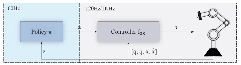
Figure 1: The policy outputs an action $a$, which is then transformed into joint torques $\tau$ using a select controller $f_{as}$. The policy and controller receive feedback from the environment. Each action space is defined by the choice of the controller and the way the action is treated in the controller. The policy runs at a 60Hz frequency and the controller runs at a frequency of 120Hz and 1KHz in the simulation and the real world respectively.

III Methods

In robot learning, the choice of action space involves the choice of a controller and the frequency and limits of the policy outputs. The frequency directly defines the reactive capabilities of the policy, and the limits are typically given by the choice of controller and robot. In this paper, we aim to study low-level control policies. Hence, we fix the frequency of all action spaces to 60 Hz. Furthermore, we use the limits that are given by the robot for the corresponding control variables.

III-A Reinforcement Learning

RL automates policy learning by maximizing the cumulative reward in a given environment [26]. Tasks are usually formulated as Markov Decision Processes (MDP). A finite-horizon, discounted MDP is defined by the tuple $\mathcal{M}=(\mathcal{S},\mathcal{A},\mathcal{P},r,\rho_{0},\gamma,T)$, where $\mathcal{S}$ and $\mathcal{A}$ are the state and action spaces respectively, $\mathcal{P}:\mathcal{S}\times\mathcal{A}\to\mathcal{S}$ is the transition dynamics, and $r:\mathcal{S}\times\mathcal{A}\to\mathbb{R}$ the reward. In addition, we have an initial state distribution $\rho_{0}$, a discount factor $\gamma\in[0,1]$, and a horizon length $T$. The optimal policy $\pi:\mathcal{S}\to P(\mathcal{A})$ maximizes the expected discounted reward:

$$J(\pi)=E_{\pi}\left[\sum_{t=0}^{T-1}\gamma^{t}r(s_{t},a_{t})\right].$$ (1)

In this study, we use the proximal policy optimization (PPO) algorithm [24] for learning manipulation policies. This choice is based on the popularity of this algorithm in recent works on sim-to-real transfer [27, 1, 10, 13, 28].

III-B Action Spaces

For arm manipulation, one of the most native RL action spaces is one that expects joint torque (JT) commands. This corresponds to $\tau=a$, where $\tau$ is the vector of joint torques. Such an action space gives the policy full control over the robot. When given the right observations, such a policy can internally learn to control the motion and forces exerted by the robot. This action space was popular in early works using deep RL [31, 18]. However, learning a policy with this action space can be very complicated since the policy would need to either understand or implicitly handle both the kinematics and dynamics of the robot to fulfill the task. This is due to the fact that the reward is typically expressed using task space properties.

Alternatively, a low-level controller $f_{\mathrm{as}}:\mathcal{A}\longmapsto T$ can be integrated in the action space to convert higher-level policy actions into the space of joint torques $T$ of the robot. This concept is illustrated in Figure 1.

Configuration action spaces consist of all action spaces that expect a configuration-space action from the policy. At the center of all these action spaces is the same controller, namely a joint impedance controller (JIC). JIC regulates the behavior of a robot manipulator’s joints and allows specifying desired stiffness, damping, and inertia characteristics for each joint. This allows the robot to be compliant with its environment. The JIC control law is the following:

$$\tau =f_{\mathrm{JIC}}(a)$$ (2)

$$\tau =K(q_{d}-q)+D(\dot{q_{d}}-\dot{q}),$$ (3)

where $\tau$ denotes the commanded joint torque, $q_{d}$ and $\dot{q_{d}}$ denote the desired joint positions and velocities respectively, and $q$ and $\dot{q}$ denote the actual joint positions and velocities of the robot given as feedback. $K$ and $D$ are the stiffness and damping matrices. In practice, we use isotropic gains, i.e., these matrices are diagonal. Given this control law, we can define two different base configuration action spaces:

• Joint Velocities (JV): sets $f_{\mathrm{JV}}\leftarrow f_{\mathrm{JIC}}$, and $\dot{q_{d}}=s(a)$ and $q_{d}$ is a first-order integration of $\dot{q_{d}}$;

• Joint Position (JP): sets $f_{\mathrm{JP}}\leftarrow f_{\mathrm{JIC}}$, and $q_{d}=s(a)$ and $\dot{q_{d}}$ is a first-order differentiation of $q_{d}$.

$s(a)$ is a function that scales the action vector to the limits of the corresponding output vector. The differentiation and integration steps are often ignored in RL action space implementations, despite being present in the most common robot control libraries. Not including these steps in the simulation would create an additional sim-to-real gap.

Task action spaces are defined using variables that are in the task/Cartesian space of the robot. In the absence of accurate system identification, we can use the following Cartesian impedance controller:

$$\tau=J(q)^{T}\bigl{(}K(x_{d}-x)+D(\dot{x_{d}}-\dot{x})\bigr{)},$$ (4)

where $J(q)$ is the Jacobian matrix for the current robot configuration $q$, relating joint velocities to Cartesian velocities, $x_{d}$ and $\dot{x_{d}}$ are the desired Cartesian poses and velocities, $x$ and $\dot{x}$ are the current Cartesian poses and velocities respectively. However, this formulation can be tricky to use when the $x_{d}$ and $\dot{x_{d}}$ are generated by an RL policy. This is due to the non-smooth nature of RL action trajectories. Of course, this problem can be handled by introducing interpolators or cubic spline fitting. But such solutions involve multiple design choices and hyperparameters, meaning that an ideal solution is task-specific. Instead, we transform the Cartesian actions into joint velocities, and then use a joint impedance controller. We found this approach to be very good at handling the non-smooth policy actions, without introducing any additional sim-to-real gap. We have two base task action spaces:

• Cartesian Velocities (CV): sets $\dot{x_{d}}\leftarrow s(a)$, transforms $\dot{x_{d}}$ into $\dot{q_{d}}$ using inverse kinematics (IK), and then uses the $f_{\mathrm{JIC}}$ in the same fashion as in the joint velocities action space;

• Cartesian Position (CP): sets $x_{d}\leftarrow s(a)$, and then uses a proportional control to obtain $\dot{x_{d}}$ from $x_{d}$. This step naturally results in smooth $\dot{x_{d}}$. Given $\dot{x_{d}}$, this action space proceeds as in the CV action space.

We use the pseudoinverse IK method with a null-space controller that pushes the joints toward their default positions.

Delta action spaces are based on the base action spaces defined previously. In contrast to the base action spaces, delta action spaces set the control targets $v_{d}$ relative to the current system feedback or to the control targets of the previous policy step. This distinction creates two classes of delta action spaces:

• One-step Integrator (OI$\Delta$): uses the robot feedback $v$ to set $v_{d}\leftarrow v+c\cdot a\cdot dt$;

• Multi-step Integrator (MI$\Delta$): recurrently sets $v_{d}\leftarrow v_{d}+c\cdot a\cdot dt$.

Depending on the choice of base action space, $v_{d}$ is a control target vector, and can correspond to $q_{d}$, $\dot{q_{d}}$, $x_{d}$, or $\dot{x_{d}}$. Similarly, $v$ is a control feedback vector, and can correspond to $q$, $\dot{q}$, $x$, or $\dot{x}$. $dt$ is the step duration and $c$ is a positive constant hyperparameter. Instead of the scaling performed in non-delta base action spaces, we clip the target $v_{d}$ to the limits of the corresponding output space after updating it. This means that each base (configuration or task) action space has two additional variants, resulting in 12 action spaces, not including the joint torques action space. Despite relying on the base action spaces, the delta variants have their unique properties. For instance, due to the relative changes in the control targets, the magnitude of the target change in one step is bound by $c\cdot dt$ given that $a\in[-1,1]$. This property can be helpful in imposing smoothness constraints on control target trajectories, even if policy output is unconstrained. Additionally, if we set $c$ to be the positive bound of the derivative of the corresponding control feedback variable $v$, each delta action space would approximately be equivalent to an action space of a higher-order derivative than its base action space. For instance, a delta joint velocity action space would be approximately similar to a joint acceleration action space. However, when sampling actions $a$ from a uniform distribution, the resulting distribution of control targets can differ between a delta action space and the base action space it approximates (e.g. $\Delta$JP and JV). The clipping can also lead to more probability mass on the borders of the $v_{d}$ space.

III-C Metrics

For each action space, we aim to assess its training performance, resulting sample efficiency, emerging properties such as the usability in the real-world environment, and the sim-to-real gap it creates. Therefore, we propose multiple metrics to quantify these different aspects. For assessing training performance, we look at the episodic rewards (ER) in simulation. This metric can also show us the sample efficiency of the different action spaces.

To assess the emerging properties of each policy, we look at the number of times it violates robot constraints, such as the joint acceleration and jerk constraints. This is especially important since simulated environments rarely have any mechanisms for enforcing these constraints. In contrast, real-world robot control implementations can include rate limiters, which ensure that the control targets would not result in violations of these constraints. Hence, a policy trained in simulation without such mechanisms could learn to violate them for the sake of exploration. Implementing these mechanisms in simulation, on the other hand, can also hinder the policy training since these mechanisms typically break the Markov assumption. To quantify this property, we use the expected constraints violations (ECV) defined as

$$\mathrm{ECV}(\pi)=E_{s,a\sim\pi}\left[\mathds{1}\left(\sum_{c\in\mathcal{C}}c(s,a)>0\right)\right],$$ (5)

where $\mathds{1}$ is an indicator function, $\mathcal{C}$ is the set of all constraints, and each constraint function $c(s,a)$ returns 1 for violated constrained and 0 otherwise. Furthermore, we report the normalized tracking error (NTE) as a measure of the feasibility of the policy’s actions in the environment,

$$\mathrm{NTE}(\pi)=E_{s,a\sim\pi}\frac{|v_{d,t}-v_{t+1}|}{v_{\mathrm{max}}-v_{\mathrm{min}}},$$ (6)

where $v_{\mathrm{min}}$ and $v_{\mathrm{max}}$ are respectively the lower and upper bounds of the control variable $v$. NTE is useful for analysing why certain action spaces result in better transfer. A high value means that the policy outputs actions that are hard to achieve in one control step. This could create an additional sim-to-real gap since control targets that are not fulfilled in one step can be tracked differently in simulated and real environments due to the gap in dynamics. We also report the task accuracy (ACC) measured by the Euclidean distance to the goal. This metric gives a more detailed view of the performance of a policy than just the success rate.

To assess the sim-to-real gap of each action space we report the offline trajectory error (OTE) in configuration and task spaces. This metric measures the joint trajectory error when replaying, in simulation, the actions produced by the policy when queried in the real world,

$$\mathrm{OTE}(\pi)=E_{a,q_{\mathrm{real}}\sim\mathcal{D}_{\mathrm{real}}}|q_{\mathrm{sim}}-q_{\mathrm{real}}|,$$ (7)

where $a$ and $q_{\mathrm{real}}$ are actions and joint configurations that are sampled from the dataset $\mathcal{D}_{\mathrm{real}}$. The latter is collected by playing a policy $\pi$ in the real-world, and $q_{\mathrm{sim}}$ is the joint configuration obtained when executing $a$ in simulation in an open-loop fashion, i.e. without a policy.

IV Experiments

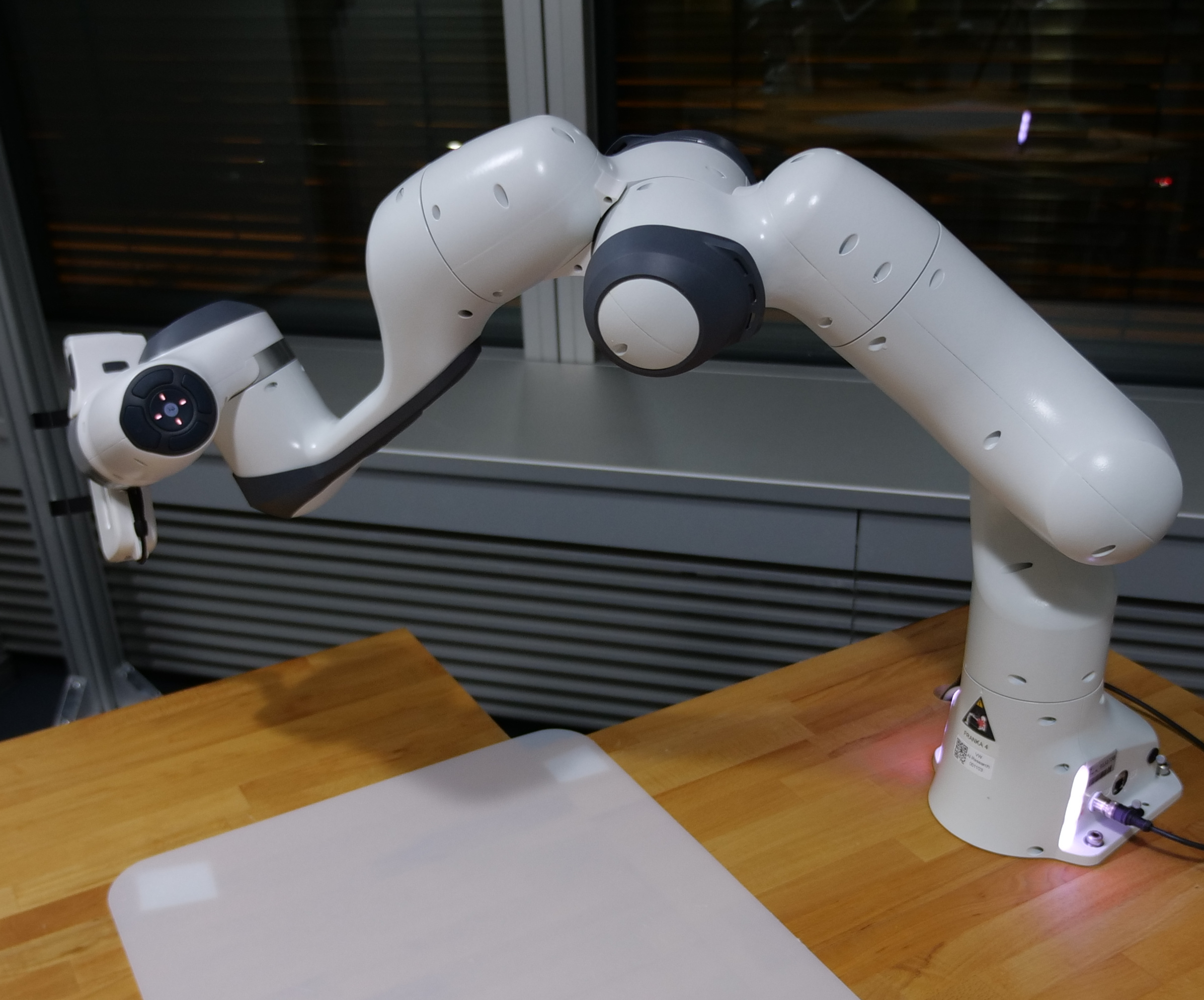
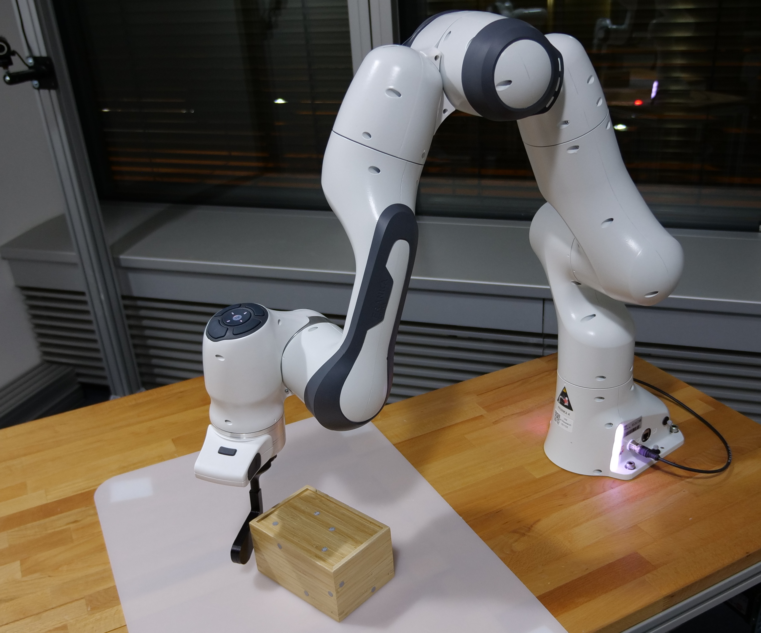
Figure 2: We show our real-world robot setup for the reaching (left) and the pushing (right) tasks.

We design experiments to understand the role of different characteristics of the action space on learning efficiency, sim-to-real gap, emerging properties, and sim-to-real transfer. Throughout this section, we pose different questions related to these topics, and answer them to the best of our capability based on empirical analysis. To answer these questions we evaluate all action spaces on two arm manipulation tasks, using the 7-degree-of-freedom Franka Emika Panda robot. The first task is goal reaching. At the beginning of each episode, a Cartesian goal is sampled in the workspace of the robot, and the policy needs to move the end-effector towards that goal. This task is ideal for studying the behavior of policies from all action spaces in the lack of force interactions with the robot’s environment. The second task is object pushing. At the beginning of each episode, a goal position is sampled in a predefined area on the table. The policy needs to push a wooden box towards that goal. This task involves moving an external object. Unlike the reaching task, pushing requires physical interaction with the environment. It allows us to understand the reactive capabilities of each action space and whether it creates any sim-to-real gap that hinders the transfer of the interaction behavior. During policy training for pushing in simulation, we perform domain randomization on the box’s friction and mass parameters. The real-world setup for both tasks is shown in Figure 2. In both tasks, the observation space of the policy consists of joint positions, joint velocities, end-effector Cartesian position, and the goal position. Additionally, in the pushing task the policy has access to the object’s position and orientation. We train PPO policies in a simulated environment, using NVIDIA’s Isaac-sim simulator [20].

Action	Reaching (Epochs)							Pushing (Epochs)
space	25		50		75			25		50		75
JP	$470$ $\pm$	$7$	$478$ $\pm$	$3$	$481$ $\pm$	$3$		$15$ $\pm$	$5$	$122$ $\pm$	$82$	$208$ $\pm$	$116$
OI$\Delta$JP	$474$ $\pm$	$1$	$472$ $\pm$	$1$	$464$ $\pm$	$3$		$338$ $\pm$	$35$	$376$ $\pm$	$17$	$388$ $\pm$	$21$
MI$\Delta$JP	$387$ $\pm$	$14$	$425$ $\pm$	$11$	$436$ $\pm$	$6$		$155$ $\pm$	$114$	$175$ $\pm$	$150$	$114$ $\pm$	$133$
JV	$438$ $\pm$	$13$	$459$ $\pm$	$4$	$455$ $\pm$	$7$		$381$ $\pm$	$17$	$400$ $\pm$	$9$	$379$ $\pm$	$39$
OI$\Delta$JV	$453$ $\pm$	$3$	$457$ $\pm$	$2$	$461$ $\pm$	$3$		$332$ $\pm$	$74$	$385$ $\pm$	$27$	$359$ $\pm$	$42$
MI$\Delta$JV	$455$ $\pm$	$4$	$465$ $\pm$	$3$	$465$ $\pm$	$1$		$243$ $\pm$	$157$	$383$ $\pm$	$43$	$381$ $\pm$	$16$
JT	$479$ $\pm$	$2$	$476$ $\pm$	$3$	$474$ $\pm$	$3$		$71$ $\pm$	$158$	$116$ $\pm$	$182$	$187$ $\pm$	$257$
CP	$456$ $\pm$	$7$	$467$ $\pm$	$2$	$465$ $\pm$	$4$		$300$ $\pm$	$157$	$322$ $\pm$	$167$	$379$ $\pm$	$34$
OI$\Delta$CP	$470$ $\pm$	$2$	$467$ $\pm$	$3$	$466$ $\pm$	$3$		$365$ $\pm$	$26$	$387$ $\pm$	$13$	$395$ $\pm$	$5$
MI$\Delta$CP	$409$ $\pm$	$9$	$441$ $\pm$	$2$	$442$ $\pm$	$3$		$283$ $\pm$	$29$	$311$ $\pm$	$7$	$307$ $\pm$	$21$
CV	$478$ $\pm$	$2$	$476$ $\pm$	$2$	$470$ $\pm$	$2$		$410$ $\pm$	$8$	$416$ $\pm$	$8$	$423$ $\pm$	$5$
OI$\Delta$CV	$471$ $\pm$	$3$	$468$ $\pm$	$4$	$464$ $\pm$	$5$		$396$ $\pm$	$15$	$422$ $\pm$	$8$	$415$ $\pm$	$13$
MI$\Delta$CV	$467$ $\pm$	$2$	$467$ $\pm$	$2$	$462$ $\pm$	$3$		$393$ $\pm$	$29$	$417$ $\pm$	$12$	$414$ $\pm$	$7$

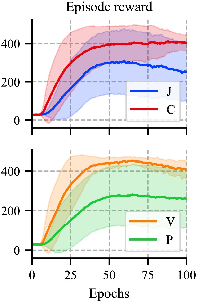
Figure 3: We compare the episodic reward (ER) obtained during training in simulation for all the studied action spaces. These include joint (J) and Cartesian (C) action spaces for position (P), velocity (V) and torque (T) control. They also include delta ($\Delta$) spaces, with one-step (OI) and multi-step (MI) target integration schemes. Left: Comparing all action spaces while picking only the best-performing delta variants. The rewards are shown for reaching and pushing at multiple stages of the training process. Right: We show learning curves for the pushing task and aggregate action spaces according to some of the characteristics named above.

The results discussed in this paper are based on 250 agents with different action spaces and different tasks. However, prior to the final training runs (of the 250 agents) we spent considerable time optimizing other hyperparameters, such as learning rates or different reward scales and terms, to guarantee consistency and a fair comparison over all action spaces. We matched the simulation to the real environment to the best of our knowledge, eliminating sim-to-real gaps where possible. This includes, for example, matching the stiffness of the impedance controllers, sharing implementations for each action space across both environments, and finding good velocity limits that allow for safe transfer of policies. This tuning process required training more than 20,000 agents in simulation and testing more than a 1500 agents in the real world. After training, we evaluate the learned policies in both tasks in simulation and in the real world. For reaching, we use a fixed grid of target goals that span the feasible workspace of the robot. For pushing, we randomly sample goal positions and use the object position from the previous episode as the initial one from the new run. We only manually reset the object’s position whenever it gets outside of the predefined area it was trained to operate in or when the policy fails to push the object away from its starting location once. We introduced the latter intervention to avoid heavily skewing the data by randomly sampling a difficult-to-handle initial object position. In both training and evaluation, we run the simulation at 120 Hz and we use action repeat to work with the policy output at 60 Hz. On the real robot, we need an additional low-level safety controller running at 1 kHz, which also repeats the actions from the policy. In all action spaces except torque we additionally use a 5 Hz low-pass filter and a rate limiter to conform to motion limits given by the robot. We tried implementing the rate limiter in simulation as well, however, the policy learning deteriorated massively, which we attribute to the rate limiter breaking the Markov property. For the policy network, we use a 4-layer feed-forward neural network for all action spaces.

Does the choice of action space affect the exploration behavior during training in simulation?
We first examine the training performance in simulation. The results can be seen in the table in Figure 3. The episodic rewards are not directly representative of the success rate of the policies. This can be seen when comparing the rewards from Figure 3 to the success rates shown in Table I. Therefore, we mostly focus on sample efficiency in the current analysis. Since different action spaces have different characteristics, we aim to understand the global effect of these characteristics on the sample efficiency during training. First, we compare Cartesian and joint action spaces. In the reaching task, both action space groups behave almost identically. However, in the pushing task, Cartesian action spaces seem to have an advantage in terms of sample efficiency and maximum reached reward, as can be seen in the top right plot in Figure 3. This result is most likely due to the spatial nature of the pushing task, which gives Cartesian action spaces a natural advantage in exploration.

We next compare the order of derivative of the action space, i.e. positions vs. velocities vs. torques. Among joint action spaces, joint velocity and its derivatives have the overall best performance in both tasks. These action spaces show better sample efficiency and converge to higher reward regions than their counterparts in the joint action space group as can be seen in the bottom right plot in Figure 3. JP reaches the highest reward in reaching but struggles massively in pushing. The same tendency can be observed for Cartesian action spaces, i.e. velocity action spaces perform better in terms of sample efficiency and final rewards. The joint torque action space is the fastest one to converge in the reaching task, however, it fails to solve the pushing task reliably within the same data budget.

We also compare base action spaces with the two different kinds of delta action spaces. We observe that multi-step integration delta action spaces consistently perform the worst, while one-step methods seem to have a slight advantage. This tendency is less pronounced in the velocity action spaces, with MI$\Delta$JV being consistently one of the best-performing joint action spaces in both tasks in simulation. Hence, the current simulation data does not conclusively favor any of these characteristics (non-delta, OI and MI).

Overall, we note that Cartesian velocity (CV) is the best-performing action space in simulation. The worst one is multi-step-integration joint position action space.

TABLE I: Sim-to-real transfer evaluation. We evaluate the success rate (SR) in simulation and the real-world environment, the task accuracy (ACC), the expected constraints violations (ECV), and the offline trajectory error (OTE).

Action	Reaching											Pushing
space	SR (sim) $\uparrow$		SR (real) $\uparrow$		ACC [cm] $\downarrow$		ECV $\downarrow$		OTE [rad] $\downarrow$			SR (sim) $\uparrow$		SR (real) $\uparrow$		ACC [cm] $\downarrow$		ECV $\downarrow$
JP	$100$   $\pm$	$0$	$6$  $\pm$	$6$	$1.76$ $\pm$	$0.14$	$100$ $\pm$	$0$	$0.22$ $\pm$	$0.01$		$87$  $\pm$	$12$	$4$   $\pm$	$0$	$4.23$ $\pm$	$0.66$	$100$ $\pm$	$0$
OI$\Delta$JP	$100$   $\pm$	$0$	$86$  $\pm$	$9$	$1.59$ $\pm$	$0.16$	$14$ $\pm$	$1$	$0.45$ $\pm$	$0.01$		$99$  $\pm$	$3$	$48$   $\pm$	$12$	$3.16$ $\pm$	$0.46$	$98$ $\pm$	$2$
MI$\Delta$JP	$100$   $\pm$	$0$	$69$  $\pm$	$2$	$2.14$ $\pm$	$0.13$	$0$ $\pm$	$0$	$0.03$ $\pm$	$0.00$		$90$  $\pm$	$7$	$36$   $\pm$	$3$	$3.52$ $\pm$	$0.36$	$3$ $\pm$	$1$
JV	$100$   $\pm$	$0$	$100$  $\pm$	$0$	$1.17$ $\pm$	$0.11$	$0$ $\pm$	$0$	$0.03$ $\pm$	$0.00$		$97$  $\pm$	$5$	$90$   $\pm$	$5$	$2.04$ $\pm$	$0.32$	$66$ $\pm$	$9$
OI$\Delta$JV	$100$   $\pm$	$0$	$97$  $\pm$	$5$	$1.35$ $\pm$	$0.13$	$13$ $\pm$	$11$	$0.18$ $\pm$	$0.01$		$99$  $\pm$	$3$	$88$   $\pm$	$13$	$1.56$ $\pm$	$0.13$	$75$ $\pm$	$4$
MI$\Delta$JV	$100$   $\pm$	$0$	$93$  $\pm$	$9$	$1.98$ $\pm$	$0.08$	$37$ $\pm$	$37$	$0.03$ $\pm$	$0.00$		$100$  $\pm$	$0$	$96$   $\pm$	$4$	$1.66$ $\pm$	$0.11$	$55$ $\pm$	$25$
JT	$100$   $\pm$	$0$	$64$  $\pm$	$27$	$1.97$ $\pm$	$0.25$	$22$ $\pm$	$6$	$0.52$ $\pm$	$0.03$		$40$  $\pm$	$49$	-   $\pm$	-	- $\pm$	-	$89$ $\pm$	$21$
CP	$99$   $\pm$	$2$	$25$  $\pm$	$4$	$1.71$ $\pm$	$0.29$	$26$ $\pm$	$9$	$0.16$ $\pm$	$0.01$		$100$  $\pm$	$0$	$57$   $\pm$	$9$	$2.34$ $\pm$	$0.39$	$92$ $\pm$	$3$
OI$\Delta$CP	$89$   $\pm$	$2$	$44$  $\pm$	$17$	$2.02$ $\pm$	$0.32$	$21$ $\pm$	$1$	$0.27$ $\pm$	$0.01$		$99$  $\pm$	$3$	$55$   $\pm$	$17$	$2.86$ $\pm$	$0.49$	$35$ $\pm$	$16$
MI$\Delta$CP	$100$   $\pm$	$0$	$68$  $\pm$	$2$	$1.85$ $\pm$	$0.08$	$13$ $\pm$	$4$	$0.28$ $\pm$	$0.01$		$100$  $\pm$	$0$	$73$   $\pm$	$7$	$2.36$ $\pm$	$0.14$	$99$ $\pm$	$0$
CV	$100$   $\pm$	$0$	$43$  $\pm$	$13$	$1.76$ $\pm$	$0.41$	$12$ $\pm$	$2$	$0.35$ $\pm$	$0.02$		$99$  $\pm$	$3$	$73$   $\pm$	$9$	$2.69$ $\pm$	$0.58$	$93$ $\pm$	$10$
OI$\Delta$CV	$97$   $\pm$	$2$	$24$  $\pm$	$2$	$2.13$ $\pm$	$0.13$	$17$ $\pm$	$3$	$0.40$ $\pm$	$0.01$		$99$  $\pm$	$3$	$61$   $\pm$	$19$	$2.67$ $\pm$	$0.30$	$99$ $\pm$	$0$
MI$\Delta$CV	$99$   $\pm$	$2$	$58$  $\pm$	$8$	$1.82$ $\pm$	$0.08$	$4$ $\pm$	$0$	$0.13$ $\pm$	$0.01$		$86$  $\pm$	$5$	$74$   $\pm$	$4$	$2.84$ $\pm$	$0.45$	$6$ $\pm$	$2$

What properties naturally emerge due to the choice of action space?
After training the policies in simulation we evaluate them on a real robotic setup. For the pushing task, we were not able to obtain joint torque policies that are safe to run in the real world without damaging the robot. We made multiple attempts to produce safely deployable joint torque policies, for instance, by introducing different penalties or increasing the policy’s control frequency. Despite all efforts, all joint torque policies were very jerky or aggressive when deployed on the real robot. The main difficulty was to obtain policies that are safe to deploy in a task where the end effector needs to remain in close proximity to a rigid surface, e.g. the table. Therefore, we exclude the joint toque action space from our real-world pushing experiments. The reaching task was less safety-critical. Hence, we managed to evaluate torque policies on real-world reaching. For all other action spaces, we look at their sim-to-real transfer capabilities. In Table I, we report the metrics introduced in Section III-C to quantify the sim-to-real gap and the performance in the real world. One common challenge when learning manipulation skills is to obtain smooth policies that do not violate the velocity, acceleration, and jerk constraints of the robot. Based on the results in Table I, we observe that different action spaces yield different ECV metrics. JV and its derivatives (OI$\Delta$JV and MI$\Delta$JV) have on average the lowest ECV score in both tasks. Vanilla JP results in the highest possible ECV. This means that deploying this action space in the real world would always result in some form of constraint violation. In the absence of safety mechanisms (such as rate limiters and low-pass filters) these violations can be very harmful. If such mechanisms are implemented, this behavior would increase the sim-to-real gap further because of how these violations trigger the safety mechanisms. In contrast, MI$\Delta$JP, seems to have the lowest ECV, which was also evident when evaluating this action space in the real world.

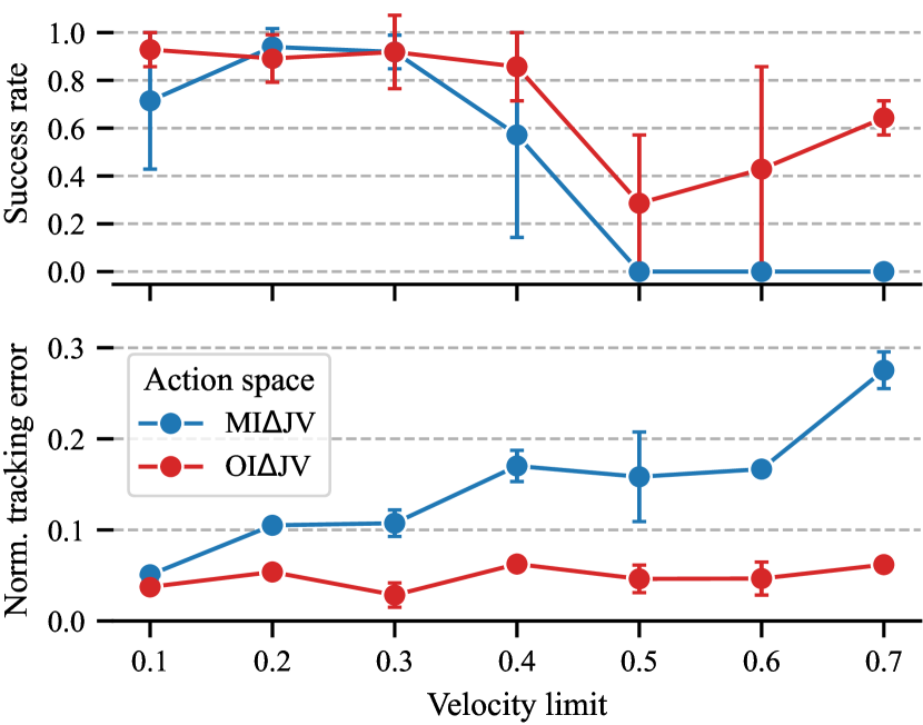
Figure 4: We show the the robustness of delta action spaces to the velocity limit hyperparameter in the pushing task on our real setup. We compare one-step and multi-step integration. The errorbars indicate one standard deviation of the respective variables.

Does the action space affect the sim-to-real gap?
First, we look at the offline trajectory error in the reaching task, which gives us a proxy measure of the sim-to-real gap. We observe that the OTE varies tremendously from one action space to another, despite the fact that the data used to compute this measure are based on the same starting and goal positions in all action spaces. This confirms that the choice of action space does indeed contribute to the sim-to-real gap. Looking closer at the results, we observe that JT exhibits the highest OTE. This is due to the behavior of this action space being dictated solely by the dynamics of the robot, which is different in simulation and in the real world. Unlike all the other action spaces, JT does not include any feedback loops outside of the policy. Based on this result, one would expect that more feedback loops should help reduce the sim-to-real gap. However, the opposite can be seen in the data. For instance, Cartesian action spaces have on average one additional feedback loop compared to the joint action spaces. Their OTE is, however, higher on average. This is due to the fact that feedback loops have different effects in simulation than in the real world. In turn, this means that a good, highly-reactive feedback loop is beneficial to overcome the dynamics gap, but adding more could potentially contribute further to the sim-to-real gap. Comparing OI$\Delta$ and MI$\Delta$ action spaces we notice that the latter consistently have a smaller OTE. Their OTE is even smaller than the corresponding base action spaces. This effect is potentially due to the integral term embedded in these action spaces. Executing the same actions results in the same final goal given to the lower-level feedback loops, which is unique compared to all other action spaces.

Which action space characteristics are good for sim-to-real transfer?
We compare the success rates in simulation and the real world. We observe that the success rate in simulation is not directly reflected in the real world. This is clear when comparing the ordering of success rates in both domains. Furthermore, we notice that certain action space characteristics are clearly advantageous for sim-to-real transfer. For instance, velocity-based action spaces tend to keep a high success rate when transferred to the real world. In contrast, position-based action spaces do not typically transfer well. This is especially the case for JP, which loses almost all of its performance when transferred. These results are consistent across both studied tasks. In addition, velocity-based action spaces are on average more accurate in fulfilling the task as can be seen when comparing the ACC score in Table I.

Additionally, we can see that delta action spaces transfer better than their corresponding base spaces. The difference between OI and MI delta action spaces depends on the task and the exact variants of the action space. However, OI$\Delta$ action spaces required less tuning than MI$\Delta$ spaces and have shown to be more robust to the choice of hyperparameters. This can be seen in Figure 4. When varying the velocity limits for $\Delta$JV action spaces, OI$\Delta$JV showed to be less sensitive to the chosen value. We attribute this to the lower tracking error of this action space as shown in the bottom plot in Figure 4. In general, OI$\Delta$ action spaces naturally lead to a lower tracking error since they integrate the policy actions into control targets based on the current feedback of the system. In contrast, MI$\Delta$ action spaces integrate the policy actions into control targets based on the previous control target. This in turn leads to a bigger gap between the control target and the state of the system, and hence a larger tracking error. While a lower NTE helps make JV action spaces more robust to hyperparameters, it has an even larger effect on the best possible transfer performance in JP action spaces, as shown in Figure 5. This tendency is also evident when comparing the base spaces, as shown in Figure 6. Finally, joint velocity show better transfer than Cartesian velocity action spaces, while the opposite is true for position-based action spaces.

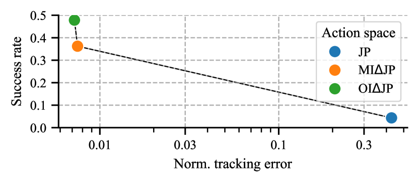
Figure 5: We compare joint position-based action spaces in the pushing task and show their influence on the normalized tracking error and the resulting effect on success rate in the real robot setup.

In summary, our data shows that two characteristics mostly influence the transfer capability of an action space. The first one is the order of the derivative of the control variables. With the exception of joint torque control, which is problematic for other reasons, an action space that controls a higher order derivative transfers better. The second characteristic is the emerging tracking error of the action space’s control variable(s). Our data strongly indicates that an action space which yields or naturally limits the tracking error transfers better. This last property can be enforced by the action space design, for instance, by reducing the magnitude of jumps of the corresponding control targets. The latter can be controlled by the scaling of the actions in delta action space, or by increasing the stiffness if the task allows. For action spaces that do not naturally allow for controlling this property, one could attempt to enforce a smaller NTE by means of rewards/penalties on the actions’ magnitude and smoothness. However, based on our experience, the tuning process for the resulting additional hyperparameters (of such reward terms) can be very difficult.

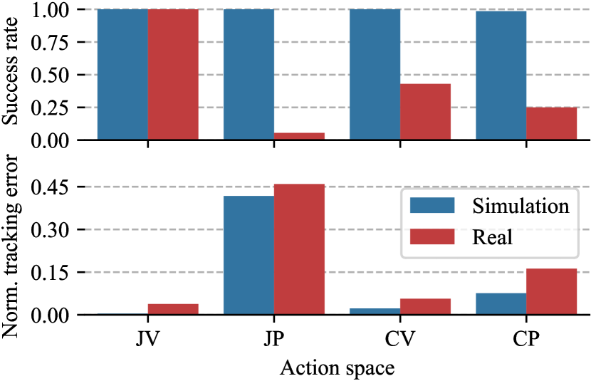
Figure 6: We show the influence of the normalized tracking error on sim-to-real transfer in terms of success rate for non-delta action spaces in the reaching task.

Is there a consistently best-performing action space?
Overall, we notice that joint velocity action spaces seem to have the best performance in sim-to-real transfer. These action spaces have on average the lowest OTE, ACC and ECV and transfer the best to the real world. They also required the least tuning to work, making them the most suited action spaces for manipulation learning (among the studied options). This result is consistent with our previous findings concerning favorable characteristics, i.e. JV-based action space benefits from a higher-quality feedback loop due to their configuration-space control, and can more easily generate high forces for interaction than position-based action space due to controlling a higher-order derivative.

V Conclusion

We studied the role of the action space in learning robotic arm manipulation skills. We designed a study that includes 13 action spaces that we used for training RL policies in simulation. We looked at the exploration behavior under the different action spaces and observed that Cartesian spaces as well as ones that control a higher-order derivative have an exploration advantage. Furthermore, we observe that different action spaces lead to different emergent properties such as the safety of their transfer and their rate of constraints violations. However, we notice that the success rate of policies in simulation does not dictate their performance in the real world. Our study further shows that the characteristics that mostly affect the sim-to-real transfer are the order of derivative and the emerging tracking error of the action space. Joint velocity-based action spaces show very favorable properties, and overall the best transfer performance. Our results show that the choice of action space plays a central role in learning manipulation policies and the transfer of such policies to the real world. Future work can build on our findings for selecting action spaces for manipulation applications or for designing more suitable alternatives.

We provide more details concerning our environments. For the reaching task, we define the reward function

$$r_{reach}(s_{t},a_{t}) =rew_{reach}(s_{t},a_{t})-pen_{reach}(s_{t},a_{t})$$

$$rew_{reach} =r_{dist}+r_{exact}$$

$$pen_{reach} =r_{vel}+r_{smooth}+r_{neutral}+r_{limit}$$

$$r_{dist}(s_{t},a_{t}) =\lambda_{r}\cdot\frac{1}{1+\left\lVert s_{t}-g\right\rVert_{2}^{2}}$$

$$r_{exact}(s_{t},a_{t}) =\mathds{1}(\left\lVert s_{t}-g\right\rVert_{2}<\epsilon)(\lambda_{\epsilon}+\frac{1}{1+100\dot{q}^{2}})$$

$$r_{vel}(s_{t},a_{t}) =\lambda_{q}\cdot\left\lVert\dot{q}_{t}\right\rVert_{2}^{2}$$

$$r_{neutral}(s_{t},a_{t}) =\lambda_{n}\cdot\left\lVert q_{def}-q\right\rVert_{2}$$

$$r_{limit}(s_{t},a_{t}) =\lambda_{l}\cdot e^{-30(q-q_{lim})^{2}}$$

$$r_{smooth}(s_{t},a_{t}) =\lambda_{s}\cdot\left\lVert a_{t}-a_{t-1}\right\rVert_{2},$$

where we use the Euclidean norm as a distance metric. $g$ is the end-effector goal position, $q_{def}$ is the default joint positions vector, $\epsilon$ is a small positive constant, $\lambda_{r}$ and $\lambda_{\epsilon}$ scale the reach and exact reach reward, $\lambda_{q}$ and $\lambda_{s}$ are positive scalars for the penalties on the velocity magnitude and smoothness of the action respectively and $\mathds{1}$ is an indicator function, $lamda_{n}$ is a scalar for the penalties on divergence from the default joint position, and $\lambda_{l}$ is a scalar for the joint limit avoidance penalty. For pushing we have a different reward,

$$r_{\text{push}}(s_{t},a_{t}) =rew_{\text{push}}(s_{t},a_{t})-pen_{\text{push}}(s_{t},a_{t})$$

$$rew_{\text{push}} =r_{dist}+r_{exact}+r_{\text{push}}$$

$$pen_{\text{push}} =r_{vel}+r_{smooth}+r_{neutral}+r_{limit}+r_{col}$$

$$r_{col}(s_{t},a_{t}) =\lambda_{c}\cdot\mathds{1}(z_{ee}<0.02),$$

where $\lambda_{c}$ is a scalar for the table collision penalty, $z_{ee}$ is the end-effector’s z-position, $r_{dist}$ and $r_{exact}$ use the object position as goal, and $r_{\text{push}}$ is defined exactly as $r_{dist}$, but measures the distance between the object’s position and the pushing goal position.

Appendix A Recommendations & Takeaways

References

- [1] Ilge Akkaya, Marcin Andrychowicz, Maciek Chociej, Mateusz Litwin, Bob McGrew, Arthur Petron, Alex Paino, Matthias Plappert, Glenn Powell, Raphael Ribas, et al. Solving rubik’s cube with a robot hand. arXiv preprint arXiv:1910.07113, 2019.
- [2] Elie Aljalbout, Ji Chen, Konstantin Ritt, Maximilian Ulmer, and Sami Haddadin. Learning vision-based reactive policies for obstacle avoidance. In Conference on Robot Learning, pages 2040–2054. PMLR, 2021.
- [3] Elie Aljalbout, Maximilian Karl, and Patrick van der Smagt. Clas: Coordinating multi-robot manipulation with central latent action spaces. In Learning for Dynamics and Control Conference, pages 1152–1166. PMLR, 2023.
- [4] Marvin Alles and Elie Aljalbout. Learning to centralize dual-arm assembly. Frontiers in Robotics and AI, 9:830007, 2022.
- [5] Arthur Allshire, Roberto Martín-Martín, Charles Lin, Shawn Manuel, Silvio Savarese, and Animesh Garg. Laser: Learning a latent action space for efficient reinforcement learning. In 2021 IEEE International Conference on Robotics and Automation (ICRA), pages 6650–6656. IEEE, 2021.
- [6] Shikhar Bahl, Mustafa Mukadam, Abhinav Gupta, and Deepak Pathak. Neural dynamic policies for end-to-end sensorimotor learning. Advances in Neural Information Processing Systems, 33:5058–5069, 2020.
- [7] Cristian Camilo Beltran-Hernandez, Damien Petit, Ixchel Georgina Ramirez-Alpizar, Takayuki Nishi, Shinichi Kikuchi, Takamitsu Matsubara, and Kensuke Harada. Learning force control for contact-rich manipulation tasks with rigid position-controlled robots. IEEE Robotics and Automation Letters, 5(4):5709–5716, 2020.
- [8] Miroslav Bogdanovic, Majid Khadiv, and Ludovic Righetti. Learning variable impedance control for contact sensitive tasks. IEEE Robotics and Automation Letters, 5(4):6129–6136, 2020.
- [9] João Borrego, Pechirra de Carvalho Borrego, Plinio Moreno López, José Alberto Rosado, and Luís M. M. Custódio. Mind the gap! bridging the reality gap in visual perception and robotic grasping with domain randomisation. 2018.
- [10] Yevgen Chebotar, Ankur Handa, Viktor Makoviychuk, Miles Macklin, Jan Issac, Nathan Ratliff, and Dieter Fox. Closing the sim-to-real loop: Adapting simulation randomization with real world experience. In 2019 International Conference on Robotics and Automation (ICRA), pages 8973–8979. IEEE, 2019.
- [11] Helei Duan, Jeremy Dao, Kevin Green, Taylor Apgar, Alan Fern, and Jonathan Hurst. Learning task space actions for bipedal locomotion. In 2021 IEEE International Conference on Robotics and Automation (ICRA), pages 1276–1282. IEEE, 2021.
- [12] Aditya Ganapathi, Pete Florence, Jake Varley, Kaylee Burns, Ken Goldberg, and Andy Zeng. Implicit kinematic policies: Unifying joint and cartesian action spaces in end-to-end robot learning. In 2022 International Conference on Robotics and Automation (ICRA), pages 2656–2662. IEEE, 2022.
- [13] Ankur Handa, Arthur Allshire, Viktor Makoviychuk, Aleksei Petrenko, Ritvik Singh, Jingzhou Liu, Denys Makoviichuk, Karl Van Wyk, Alexander Zhurkevich, Balakumar Sundaralingam, et al. Dextreme: Transfer of agile in-hand manipulation from simulation to reality. In 2023 IEEE International Conference on Robotics and Automation (ICRA), pages 5977–5984. IEEE, 2023.
- [14] Eric Heiden, David Millard, Erwin Coumans, and Gaurav S. Sukhatme. Augmenting differentiable simulators with neural networks to close the sim2real gap. ArXiv, abs/2007.06045, 2020.
- [15] Jemin Hwangbo, Joonho Lee, Alexey Dosovitskiy, Dario Bellicoso, Vassilios Tsounis, Vladlen Koltun, and Marco Hutter. Learning agile and dynamic motor skills for legged robots. Science Robotics, 4(26):eaau5872, 2019.
- [16] Mrinal Kalakrishnan, Ludovic Righetti, Peter Pastor, and Stefan Schaal. Learning force control policies for compliant manipulation. In 2011 IEEE/RSJ International Conference on Intelligent Robots and Systems, pages 4639–4644. IEEE, 2011.
- [17] Elia Kaufmann, Leonard Bauersfeld, and Davide Scaramuzza. A benchmark comparison of learned control policies for agile quadrotor flight. In 2022 International Conference on Robotics and Automation (ICRA), pages 10504–10510. IEEE, 2022.
- [18] Timothy P Lillicrap, Jonathan J Hunt, Alexander Pritzel, Nicolas Heess, Tom Erez, Yuval Tassa, David Silver, and Daan Wierstra. Continuous control with deep reinforcement learning. arXiv preprint arXiv:1509.02971, 2015.
- [19] Jianlan Luo, Eugen Solowjow, Chengtao Wen, Juan Aparicio Ojea, Alice M Agogino, Aviv Tamar, and Pieter Abbeel. Reinforcement learning on variable impedance controller for high-precision robotic assembly. In 2019 International Conference on Robotics and Automation (ICRA), pages 3080–3087. IEEE, 2019.
- [20] Viktor Makoviychuk, Lukasz Wawrzyniak, Yunrong Guo, Michelle Lu, Kier Storey, Miles Macklin, David Hoeller, Nikita Rudin, Arthur Allshire, Ankur Handa, et al. Isaac gym: High performance gpu-based physics simulation for robot learning. arXiv preprint arXiv:2108.10470, 2021.
- [21] Roberto Martín-Martín, Michelle A Lee, Rachel Gardner, Silvio Savarese, Jeannette Bohg, and Animesh Garg. Variable impedance control in end-effector space: An action space for reinforcement learning in contact-rich tasks. In 2019 IEEE/RSJ International Conference on Intelligent Robots and Systems (IROS), pages 1010–1017. IEEE, 2019.
- [22] Xue Bin Peng and Michiel Van De Panne. Learning locomotion skills using deeprl: Does the choice of action space matter? In Proceedings of the ACM SIGGRAPH/Eurographics Symposium on Computer Animation, pages 1–13, 2017.
- [23] N. Rudin, David Hoeller, Philipp Reist, and Marco Hutter. Learning to walk in minutes using massively parallel deep reinforcement learning. ArXiv, abs/2109.11978, 2021.
- [24] John Schulman, Filip Wolski, Prafulla Dhariwal, Alec Radford, and Oleg Klimov. Proximal policy optimization algorithms. arXiv preprint arXiv:1707.06347, 2017.
- [25] Laura Smith, Ilya Kostrikov, and Sergey Levine. A walk in the park: Learning to walk in 20 minutes with model-free reinforcement learning. arXiv preprint arXiv:2208.07860, 2022.
- [26] Richard S Sutton and Andrew G Barto. Reinforcement learning: An introduction. MIT press, 2018.
- [27] Jie Tan, Tingnan Zhang, Erwin Coumans, Atil Iscen, Yunfei Bai, Danijar Hafner, Steven Bohez, and Vincent Vanhoucke. Sim-to-real: Learning agile locomotion for quadruped robots. Robotics: Science and Systems, 2018.
- [28] Bingjie Tang, Michael A Lin, Iretiayo Akinola, Ankur Handa, Gaurav S Sukhatme, Fabio Ramos, Dieter Fox, and Yashraj Narang. Industreal: Transferring contact-rich assembly tasks from simulation to reality. arXiv preprint arXiv:2305.17110, 2023.
- [29] Maximilian Ulmer, Elie Aljalbout, Sascha Schwarz, and Sami Haddadin. Learning robotic manipulation skills using an adaptive force-impedance action space. arXiv preprint arXiv:2110.09904, 2021.
- [30] Patrick Varin, Lev Grossman, and Scott Kuindersma. A comparison of action spaces for learning manipulation tasks. In 2019 IEEE/RSJ International Conference on Intelligent Robots and Systems (IROS), pages 6015–6021. IEEE, 2019.
- [31] Niklas Wahlström, Thomas B Schön, and Marc Peter Deisenroth. From pixels to torques: Policy learning with deep dynamical models. arXiv preprint arXiv:1502.02251, 2015.
- [32] Zhaoming Xie, Patrick Clary, Jeremy Dao, Pedro Morais, Jonanthan Hurst, and Michiel Panne. Learning locomotion skills for cassie: Iterative design and sim-to-real. In Conference on Robot Learning, pages 317–329. PMLR, 2020.
- [33] Wenxuan Zhou, Sujay Bajracharya, and David Held. Plas: Latent action space for offline reinforcement learning. In Conference on Robot Learning, 2020.