Direct Exoplanet Detection Using Deep Convolutional Image Reconstruction (ConStruct):
A New Algorithm for Post-Processing High-Contrast Images
Abstract
We present a novel machine-learning approach for detecting faint point sources in high-contrast adaptive optics imaging datasets. The most widely used algorithms for primary subtraction aim to decouple bright stellar speckle noise from planetary signatures by subtracting an approximation of the temporally evolving stellar noise from each frame in an imaging sequence. Our approach aims to improve the stellar noise approximation and increase the planet detection sensitivity by leveraging deep learning in a novel direct imaging post-processing algorithm. We show that a convolutional autoencoder neural network, trained on an extensive reference library of real imaging sequences, accurately reconstructs the stellar speckle noise at the location of a potential planet signal. This tool is used in a post-processing algorithm we call Direct Exoplanet Detection with Convolutional Image Reconstruction, or ConStruct. The reliability and sensitivity of ConStruct are assessed using real Keck/NIRC2 angular differential imaging datasets. Of the 30 unique point sources we examine, ConStruct yields a higher S/N than traditional PCA-based processing for 67 of the cases and improves the relative contrast by up to a factor of 2.6. This work demonstrates the value and potential of deep learning to take advantage of a diverse reference library of point spread function realizations to improve direct imaging post-processing. ConStruct and its future improvements may be particularly useful as tools for post-processing high-contrast images from the James Webb Space Telescope and extreme adaptive optics instruments, both for the current generation and those being designed for the upcoming 30 meter-class telescopes.
1 Introduction
A complete statistical census of exoplanet demographics is needed to test and guide planet formation and evolutionary models (e.g., Burrows et al., 2001; Alibert et al., 2005; Gaudi et al., 2021). Planets detected with indirect methods, particularly using radial velocities or transits (Seager, 2008; Lovis et al., 2010), comprise the bulk of known discoveries. These methods are effective for finding companions at close separations to their host stars, but are less sensitive at wider orbital distances. Over the past two decades, high contrast imaging (HCI) has emerged as an effective tool to study long-period planets by probing the architectures of planetary systems from the outside in, while also enabling spectroscopic characterization of their atmospheres (Bowler, 2016; Baron et al., 2019; Nielsen et al., 2019; Vigan et al., 2021).
Dedicated hardware, including high-order adaptive optics (AO) (Guyon, 2005) and coronagraphy (Guyon et al., 2006; Oppenheimer & Hinkley, 2009), are necessary to reach the planetstar contrasts required to detect faint substellar companions with direct imaging. Advanced post-processing algorithms play a crucial role in pushing the sensitivity of imaging surveys to smaller inner-working-angles (IWAs) to maximize the scientific yield of these instruments. Central to this is accurately modeling and removing correlated quasi-static speckle noise in the imaging data. For ground-based instruments, residual atmospheric wavefront errors uncorrected with AO and instrumental aberrations produce speckle noise with correlation lengths that range between seconds and hours (Hinkley et al., 2007; Martinez et al., 2012). Efficient post-processing is especially necessary at small IWAs where speckles are often brighter and exhibit similar spatial characteristics to planetary signatures (e.g., Fitzgerald & Graham, 2005).
Post-processing strategies are tied to the observation approach. With Angular Differential Imaging (ADI) , instruments are configured to observe in pupil-tracking mode so that on-sky sources rotate deterministically around the optical axis of the instrument, while slowly evolving speckle noise realizations remain fixed in the image plane (Liu, 2004; Marois et al., 2005). Post-processing algorithms such as Locally Optimized Combination of Images (LOCI) (Lafreniere et al., 2007) and Karhunen-Loéve Image Projection (KLIP) (Soummer et al., 2012) leverage the spatial de-coupling between speckle noise and planetary signals with ADI to estimate a best-fit reconstruction of the speckle noise in each frame, conditioned on other frames in the sequence. The reconstructed images are subsequently subtracted from each respective frame, and the residual images are de-rotated and averaged to recover real sources.
Several variations and extensions of LOCI and KLIP have been developed to improve these algorithms in their original forms. For instance, at very close separations, the sky rotation is sometimes insufficient to decouple planetary signals from speckle noise, causing the reconstructed frame to partially fit any real source that might be present. To prevent excessive over-subtraction, Pueyo et al. (2012) introduced a damped version of LOCI which regularizes the least-squares reconstruction. Reference Differential Imaging (RDI) is another strategy to address over-subtraction by making use of a library of reference images (Lafrenière et al., 2009; Xie et al., 2022; Sanghi et al., 2022), or images of a reference star sampled concurrently with the target (Wahhaj et al., 2021), to create the linear reconstruction of each science frame. However, the RDI image basis is not necessarily linearly independent to the expected signal profile of an on-sky object, so some self-subtraction can still occur.
To improve the linear speckle reconstruction methods like those used in both ADI and RDI, we present a machine learning-based method for speckle noise reconstruction we call Direct Exoplanet Detection with Convolutional Image Reconstruction, or ConStruct. Our approach explicitly partitions image patches111We define image patches as small sub-frames sampled from individual ADI frames. In this work, the size of each patch is much smaller than the original ADI frame. sampled in ADI frames into hypothesized planet absentpresent sectors for post-processing. It uses the spatial speckle correlations across neighboring pixels in the planet absent sector to predict a speckle noise reconstruction, independent of potential signals, in the planet-present sector. For this, an autoencoder neural network is trained in a self-supervised learning architecture with thousands of real examples, which can be applied to science targets without further training.
By leveraging a library of archival HCI data, ConStruct is similar to RDI, but it can encode information from thousands of training examples without manually selecting a reference library of images. Our approach is motivated by algorithms developed in the machine learning community for filling corrupted or missing regions in images with deep learning, commonly known as image inpainting. Elharrouss et al. (2019) provides a review of the literature related to image inpainting.
Machine learning approaches for post-processing direct imaging data have received growing interest in recent years. A supervised learning framework for detecting faint point sources is introduced in Gonzalez et al. (2018) which uses both random forests and neural networks to classify likely candidate point sources. Similarly, in Flasseur et al. (2023) the authors use convolutional neural networks for both detection and characterization of post-processed images, generated with the PACO algorithm (Flasseur et al., 2018, 2020). Yip et al. (2019) apply generative adversarial networks to create synthetic coronagraphic image realizations. The synthetic images then train a convolutional neural network to classify regions that contain potential bright planets in single science frames. Gebhard et al. (2022) built a regularized linear model of speckle noise based on causal predictors to fill in speckle noise in a region of interest. Our approach shares some similarities; however, we utilize a highly nonlinear model to complete the speckle prediction with solely local speckle correlation.
This paper is organized as follows. In Section 2 we explain ConStruct’s principal and how it is used for detecting planetary companions. We also compare the operating mechanisms of ConStruct to those used in linear speckle reconstruction approaches like KLIP. Section 3 details the autoencoder neural network used in ConStruct as well as an additional linear correction to leverage the temporal correlations between frames in ADI sequences. In Section 4 we discuss how ConStruct is tuned to maximize the signal-to-noise ratio (SNR) of substellar sources in these data. We apply ConStruct to 30 unique point sources in data sets from the W.M. Keck Observatory’s NIRC2 imaging camera in Section 5, and compare the results with a PCA reduction approach.
2 Framework of Construct
2.1 Speckle Noise Reconstruction
In this section, we first introduce the framework behind ConStruct and place it in the context of existing approaches for processing high-contrast ADI sequences. A general region in an ADI frame can be partitioned into sub-regions and as illustrated in Figure 1. The sub-region is assumed to include only pixels from speckle noise, and contains speckle noise spatially correlated with and a potential signal from an on-sky object. The pixel-wise intensities for the frame contained in regions , , and their union, , are,
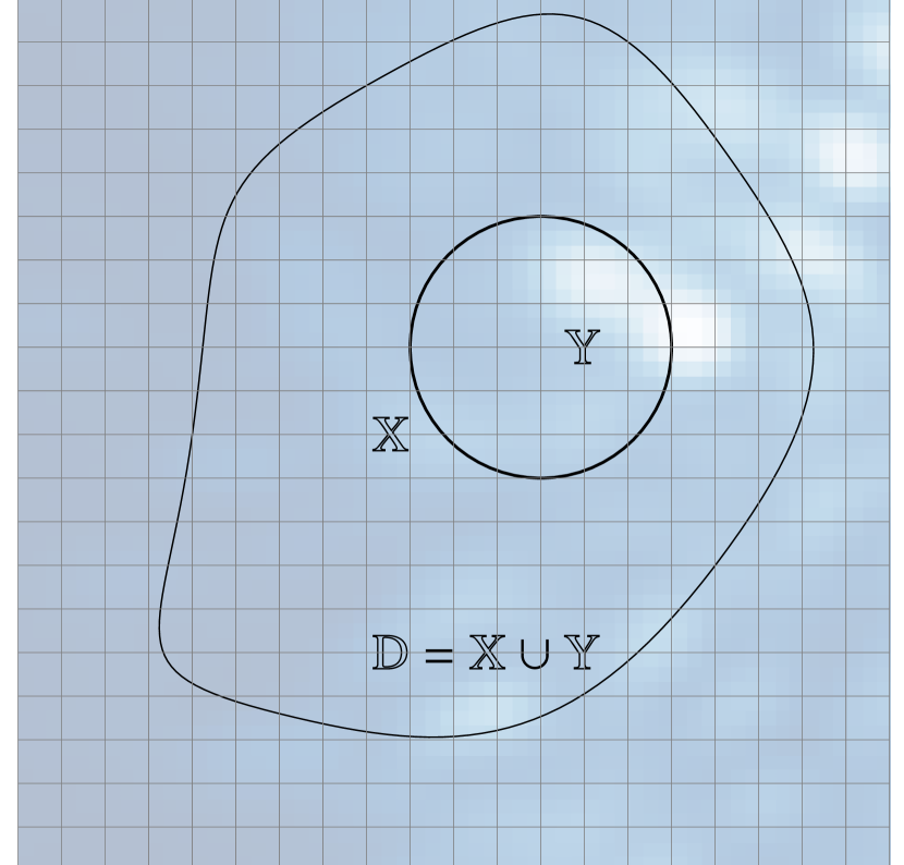
| (1) | ||||
Here, is the intensity of the speckle noise contained in region for frame , and is the intensity of the speckle noise contained in region for frame . The pixel intensities contained in are modeled as an additive combination of the speckle noise, , and a potential point source, . The term includes any irreducible uncertainty in the data. Here, we denote to be the sample statistic which is a function of the excess intensity in the region . In this formulation, if the intensity from speckle noise is known perfectly, then detecting an on-sky point source is limited only by . To that end, post-processing algorithms seek an unbiased minimum error estimate, . Principal Component Analysis (PCA)-based reconstruction approaches like KLIP estimate the weighting coefficients of an optimal low-rank image reconstruction basis matrix which together generate this estimate. Without explicitly partitioning the regions and , minimizing
| (2) |
produces a minimum mean squared error reconstruction of the region for each of the frames. Hastie et al. (2009) show that Equation 2 is equivalent to
| (3) | ||||
| (4) |
The solution to Equation (4) is found via singular value decomposition of the data matrix , where,
| (5) | ||||
| (6) |
The matrix is an orthonormal matrix and the columns contain the left-singular vectors of the decomposition. The matrix is a diagonal matrix containing the singular values of the matrix . The columns of are the right singular vectors, or principal component vectors, which are ordered in the directions of maximum variance. is obtained by truncating the columns of up to a desired integer . In PCA–based reduction approaches, the regions are sometimes partitioned into concentric annuli, sectors, or full ADI frames. Generating the speckle estimate for each region consists of two symmetric operations:
-
1.
The intensity vector is mapped onto a low-rank PCA feature space with .
-
2.
The PCA features are mapped back into the original pixel space to produce an estimate of the speckle noise in region with .
In this work, we generalize and to be two nonlinear functions and parameterized by a neural network. To alleviate partial fitting to the potential source, we explicitly exclude the region in building the reconstruction. Minimizing the cost function
| (7) |
results in the optimal nonlinear reconstruction functions and . Here, is a positive scalar, and is the number of training samples in a reference library, each indexed by an integer . We detail the architecture and implementation of this algorithm in Section 3. Note that in this formulation, the speckle noise prediction relies solely on spatial correlations exhibited between the predictor and the region of interest, .
2.2 Recovering Off-Axis Point Sources
During ADI observations, a telescope is placed in pupil tracking mode causing on-sky point sources to rotate deterministically around the optical axis of the instrument (Marois et al., 2005). Accordingly, pixel intensities in a region label a set of locations, , across the ADI sequence which will all contain a point source if it is contained in . Note that we use “” to denote the first frame of the ADI sequence. Re-arranging Equation 1, the maximum likelihood estimate of a potential point source across the set of time-dependent locations, associated to is,
| (8) |
Here, is the predicted speckle noise intensity for in the frame, which is generated through our prediction function . The operator denotes the statistical expectation taken with respect to time.
Constraining a hypothesized point source requires systematically comparing the estimated signal to its surrounding resolution elements. This is formalized in a hypothesis test where,
| (9) | ||||
with , where the operator takes the maximum value of the expected source intensity vector. This is calculated in practice by placing a circular aperture around the potential source and retrieving the maximum value within the aperture’s extent. We assume the test statistic is a Gaussian distributed random variable so that , where is the empirical root mean square (RMS) of the residual intensity in the surrounding elements. Note that we assume that residual pixel-wise intensities are independent and identically distributed (i.i.d). The optimal decision in the sense of minimizing the false negatives, subject to a fixed probability of false positives, is given by the log-likelihood ratio test,
| (10) |
Because we are assuming Gaussian statistics, Equation 10 reduces to,
| (11) |
The scaling variable is used to gate the hypothesis test as a multiplicative factor of the residual speckle RMS. Due to spatial correlations in the residual speckle intensity, the samples are not i.i.d. A more statistically sound treatment of the residual speckle noise statistics is considered in Mawet et al. (2014).
3 Autoencoder Neural Network for Image Reconstruction
3.1 Reconstruction Function Architecture
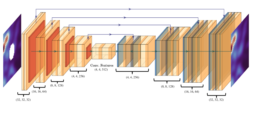
In this section, we detail how an autoencoder neural network serves as a surrogate for the functions and given in Equation 7. An autoencoder is a feed-forward neural network that reconstructs a corrupted input as its output. An encoder and decoder network portion act symmetrically to first transform a high-dimensional input into a low-dimensional feature space, and subsequently back into the original input space. ConStruct uses a fully-convolutional version of an autoencoder, similar to the U-net network (Ronneberger et al., 2015). Convolutional neural networks excel in image-based tasks, so this architecture choice is attractive for our application. We provide a graphical illustration of our network architecture in Figure 2 and show the output sizes from each block in the network.
The encoder portion of the network consists of a sequence of four convolutional blocks. Each block contains two convolutional layers, followed by a max-pooling layer. The convolutional layers create a set of feature maps by translating a convolutional filter over the output of the previous layer and applying a rectified linear activation function (ReLU) . Unique filters correspond to each feature map. Through training, the network learns a set of convolutional filters that enable it to accurately predict a corrupted, or in our case, masked region of interest. The max-pooling layer applies the maximum operator over a filter translated across the feature map. This operation downsizes each dimension of the feature map by one-half.
The decoder portion uses a set of low-dimensional convolutional features produced by the encoder to reconstruct a prediction of the speckle noise in the masked region of interest. The decoder contains four up-convolutional blocks. Similar to the encoder, each block contains two sequential convolutional layers, but these are followed by a deconvolutional layer that transforms many lower-dimensional features into one of higher dimension. The encoder features congruent to each decoder block are concatenated to the deconvolved layer, and the new set is passed into the next block. This technique, sometimes referred to as residual connections or skip connections, helps to alleviate the issue of vanishing gradients common in deep neural network architectures. The final layer in our architecture consists of a single convolutional layer with a sigmoid activation function which reconstructs a scaled speckle prediction in the masked region, along with a reconstruction of the original image region fed into the network222To facilitate stability in predicting the speckle region, all images used by ConStruct are scaled into the range of . The output from the autoencoder is re-scaled to produce the final speckle prediction.. In Appendix A, we include the layer-wise parameters for the autoencoder used by ConStruct.
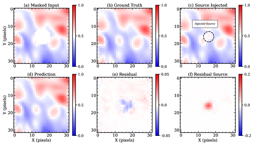
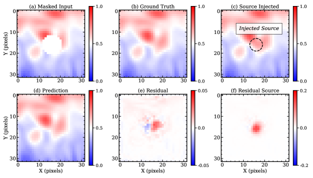
Figure 3 shows an example of using the trained autoencoder to predict speckle noise in an ADI image patch. In this example, an image patch is extracted from a frame contained in an ADI sequence of the HR 8799 system, corresponding to Sequence 9 in Table 1. A synthetic 2-D Gaussian source is injected into the center of the image patch. The central region is then masked before being fed into the network. ConStruct accurately predicts the speckle in the missing masked region, and this prediction is subtracted from the original image patch to reveal the synthetic source. In Appendix B, we included two additional prediction examples extracted from spatially disparate realizations of the the speckle field.
3.2 Data Selection
A collection of representative data is needed to train our autoencoder. We select a library of archival ADI sequences observed with the Keck NIRC2 near-infrared camera for this task. The data are downloaded from the Keck Observatory Archive (KOA), along with accompanying calibration frames. In total, 92 unique ADI sequences are used for training our algorithm.
KOA contains a large number of ADI sequences that we can potentially include for training. We downselect our sample to only include -, -, -, -, and -band filters. This choice has repercussions on which datasets we can deploy our trained algorithm: because the spatial frequency of speckle noise is wavelength dependent (Sparks & Ford, 2002), we expect our algorithm to perform best when used on ADI sequences taken with the same filters. Additionally, only data using the 400, 600, and 800 mas-diameter Lyot coronagraphs are used. The sequences were searched on the archive primarily using a list of stars with directly imaged planets and low-mass brown dwarf companions contained in Bowler (2016). Most training sequences have known point sources, but we assume that the number density of the point sources is sufficiently small across these data sets so as to not significantly bias the speckle realizations. Each sequence is visually inspected to determine its quality for training. Sequences containing saturated pixels or degraded Strehl ratios were excluded. The data used for training are detailed in Appendix C.
3.3 Processing the Training Dataset
Each of the ADI sequences used for training our network are pre-processed using standard procedures for HCI. Using dome flat calibration frames, we generate a bad-pixel mask for each sequence with the ccdproc Astropy module (Craig et al., 2017). The mask is applied to each calibration and science frame, and bad pixels are removed with nearest-neighbor interpolation. Dark subtraction and flat fielding are carried out for each frame in the science sequence. Registration is performed by centering each frame at the pixel coordinate closest central stellar Point Spread Function (PSF) , visible inside the occulting coronagraph.
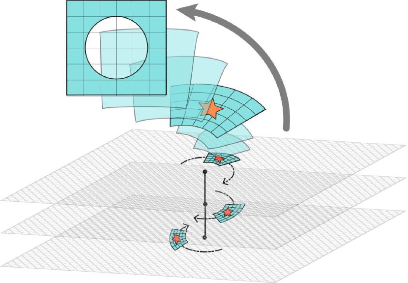
In generating training data, we draw an ADI sequence from our library by sampling a distribution who’s probability of selection is proportional to the number of frames in the respective sequence. Patch coordinates in the sequence are then uniformly sampled in azimuth, radial separation, and frame number. These define the central coordinate of a sector which is projected into a square array for training. Figure 4 illustrates the projection operation. An angular and radial width defines the dimension of each sector. Depending on the radial coordinate, we choose the angular width such that the square projection approximately maintains the number of pixels in the sector. The projection uses cubic spline interpolation. We find the information degradation resulting from this transformation is sufficiently small to not affect the performance of ConStruct.
The pixel values in each projected square array are linearly scaled between zero and one. A circular mask of zeros is applied to each of these scaled samples, corresponding to the region . The original array, , and the masked sample, , together form a training sample . We use 30,000 samples to train the network. The complete set is partitioned into a train-validation split. The prediction accuracy of the neural network is measured after each training epoch by testing it on the validation set. This is useful for imposing a stopping criterion during training: when the loss in the validation set begins to increase (i.e., the prediction accuracy decreases), the algorithm is over-fitting the training set, and training should terminate.
3.4 Autoencoder Implementation and Training
We implement our autoencoder network in Keras (Chollet et al., 2015), which is an application program interface for the TensorFlow machine learning library (Abadi et al., 2015). In training, the component of each sample is first propagated forward through the network, and the network’s prediction is subtracted from the ground truth, , to form a residual array. Repeatedly backpropagating the residual errors adjusts the autoencoder parameters such that the prediction accuracy in the masked region increases. We use a 32-sample mini-batch gradient descent with the Adam optimizer (Kingma & Ba, 2015) and a Huber loss function given as,
| (12) |
where,
The Huber loss uses the minimum squared error when deviations are small (i.e., within some defined deviation ), and minimum absolute error when deviations are large. This reduces the importance placed on outlier samples in the training process. 30 training epochs are used, and we observe that the errors in the validation set consistently decrease with all epochs. For our application, more training epochs can likely be used, but with only marginal improvement in the prediction accuracy.
3.5 Correcting the Autoencoder Prediction Residuals
We leverage the temporal correlation of speckle noise across ADI frames to further correct the residual errors of the autoencoder predictions with an L2 regularized linear regression model, otherwise known as ridge regression. In our formulation, we use the output from the autoencoder as the predictor variables for the model. For a fixed spatial region in the frame partitioned into sub-regions and , the speckle prediction from the autoencoder is . The prediction residual in the region is an additive combination of the residual speckle noise, and a potential point source,
| (13) | ||||
For each pixel in the region , we solve a regularized linear regression to correct the residuals. Let be the response variable in the regression model, where is the residual intensity for the pixel indexed by the pre-superscript in the frame. Each regression model finds the coefficients that minimize the loss function
| (14) |
which has the analytic solution,
| (15) |
Here, is the -dimensional identity matrix. is a positive scalar which acts as a tuning variable in ConStruct. Higher values of increase the bias of the regression model, but help reduce overfitting to potential companion point sources. is the design matrix, which are the horizontally stacked predictions produced by the autoencoder,
| (16) |
This is repeated for all pixels contained in region . The output of the regression step in ConStruct are the corrected residual intensities
| (17) |
where,
| (18) |
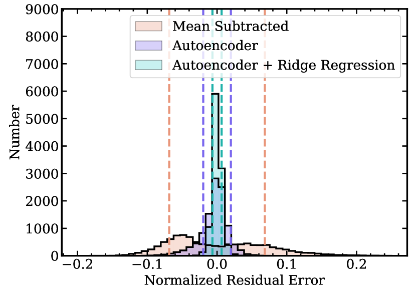
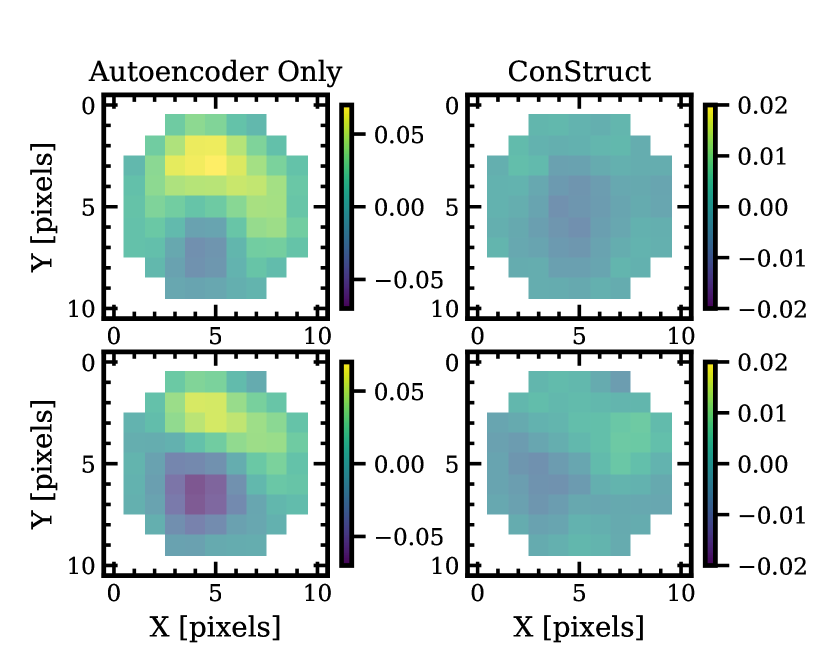
Figure 5 illustrates how the autoencoder prediction and least-squares regression step sequentially reduces the residual speckle noise. We also include two examples showing the speckle residuals in the region from the autoencoder without and with the least-squares regression in Figure 6. The estimated intensity of the potential companion point source in the region in each frame is then,
| (19) |
where denotes the column of the matrix.
3.6 Using ConStruct with ADI sequences
ConStruct uses a flexible architecture that provides sub-pixel processing capabilities with ADI sequences. Based on a user-defined resolution, and lower and upper radial processing bounds, radial and azimuthal coordinates, , are defined in the image plane that satisfy the resolution requirement. Here, we use the subscript to denote that these coordinates are located in the first frame of the ADI sequence and define the plane of the final flux map, , and S/N map, . Each coordinate labels a set of spatial patches which are centered at the set of coordinates , where is the field rotation observed up to and including frame . Post-processing is performed serially over radial resolution bins, and for each bin, the following steps are implemented:
-
1.
Each azimuthal and time coordinate defines the center of a sector area in the radial bin, and the sector is extracted and mapped to a square array, as illustrated in Figure 4. This step is parallelized for all elements in the radial bin spanning the ADI sequence.
-
2.
The extracted square arrays are each independently scaled (i.e., a unique scaling function is fit to each spatial patch) between zero and one, and the central pixel values corresponding are masked with a circular template of zeros.
-
3.
The masked arrays are fed as a batch into the autoencoder network that allows for GPU parallelization. The autoencoder reconstructs the missing regions in each patch using solely the spatial correlations with the surrounding speckle noise.
-
4.
The predictions produced by the autoencoder are re-scaled by applying the inverse of the scaling operator fit to each patch in Step #2.
-
5.
The re-scaled predictions are subtracted from the true image patches, creating a set of residual images. The residual images corresponding to a fixed azimuthal coordinate but spanning all frames, , are further corrected with ridge regression described above. This is repeated for all azimuthal elements in the radial bin.
-
6.
The corrected residuals are formed into sets that may each contain a point source, based on a label azimuthal coordinate, and the parallactic rotation of the ADI sequence. Each of these sets are denoted as . This is repeated for all azimuthal coordinates in the radial bin.
-
7.
The images in the set are averaged, and the center pixel value of the averaged array is used for the intensity of the coordinate in the final flux map, . This is repeated for all azimuthal coordinates in the radial bin.
The intensity values of contained within a radial window of pixels of are used to calculate the emperical RMS of each radial bin. The S/N values of are then
| (20) |
where denotes the emperical RMS.
= 0.0in
| Sequence # | Companion | Date (UT) | # of Frames | Int. Time (s) | Filter | Corona. (mas) | PI | S/N ConStruct | S/N PCA |
|---|---|---|---|---|---|---|---|---|---|
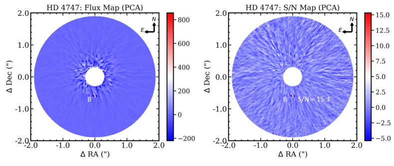
| 1 | HD 4747 B | 2015-01-09 | 39 | 2340 | 600 | Knutson | 10.9 | 15.3 | |
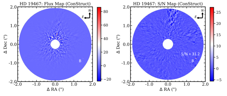
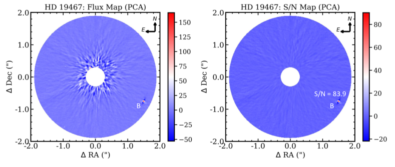
| 2 | HD 19467 B | 2011-08-30 | 50 | 1250 | 300 | Crepp | 31.2 | 83.9 | |
| 3 | HD 19467 B | 2012-08-25 | 53 | 1325 | 300 | Johnson | 11.4 | 14.6 | |
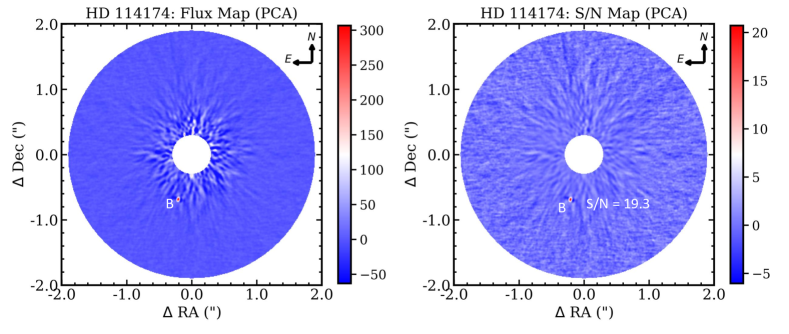
| 4 | HD 114174 B | 2011-02-22 | 36 | 720 | 300 | Crepp | 25.6 | 19.3 | |
| 5 | HD 114174 B | 2012-02-02 | 91 | 1820 | 300 | Knutson | 37.7 | 24.6 | |
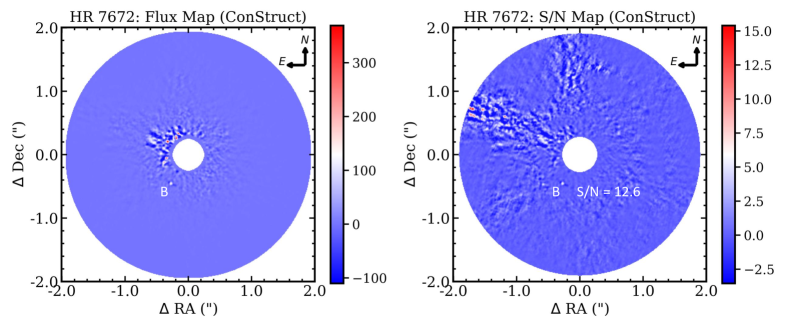
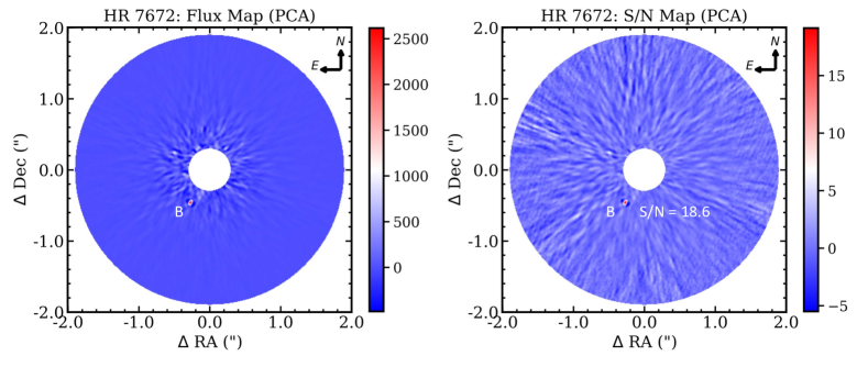
| 6 | HR 7672 B | 2011-05-15 | 30 | 450 | 300 | Carpenter | 12.6 | 18.7 | |
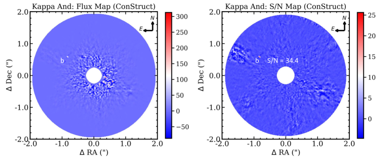
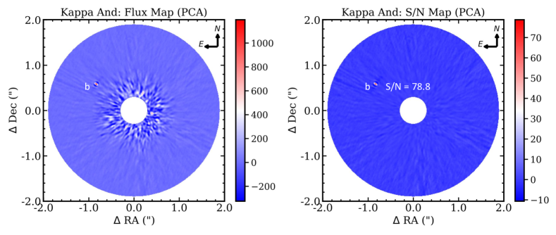
| 7 | Kappa And b | 2013-05-30 | 38 | 1520 | 400 | Carpenter | 34.4 | 78.8 | |
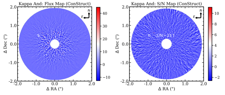
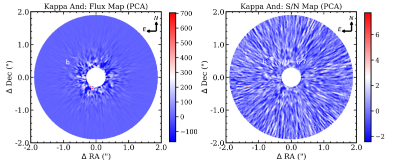
| 8 | Kappa And b | 2018-01-30 | 15 | 450 | 600 | Bowler | 11.1 | 6.7 | |
| 9 | HR 8799 b | 2010-07-13 | 70 | 1400 | 400 | Barman | 61.6 | 57.4 | |
| 9 | HR 8799 c | – | – | – | – | – | – | 48.0 | 36.5 |
| 9 | HR 8799 d | – | – | – | – | – | – | 15.0 | 9.3 |
| 9 | HR 8799 e | – | – | – | – | – | – | 2.3 | 2.7 |
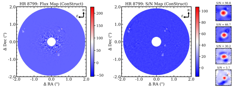
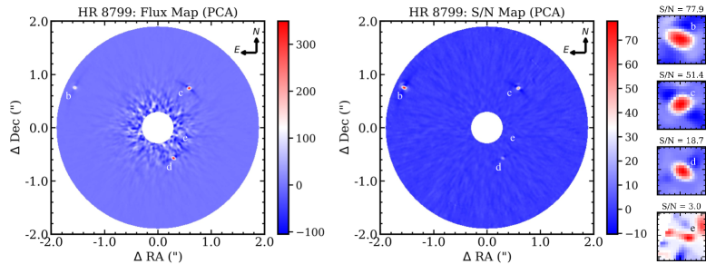
| 10 | HR 8799 b | 2011-07-21 | 148 | 2960 | 400 | Macintosh | 98.8 | 77.9 | |
| 10 | HR 8799 c | – | – | – | – | – | – | 66.7 | 51.4 |
| 10 | HR 8799 d | – | – | – | – | – | – | 30.2 | 18.7 |
| 10 | HR 8799 e | – | – | – | – | – | – | 5.7 | 3.0 |
| 11 | HR 8799 b | 2012-10-26 | 98 | 1960 | 400 | Cooray | 81.8 | 54.3 | |
| 11 | HR 8799 c | – | – | – | – | – | – | 52.8 | 25.5 |
| 11 | HR 8799 d | – | – | – | – | – | – | 21.5 | 11.5 |
| 11 | HR 8799 e | – | – | – | – | – | – | 5.0 | 4.1 |
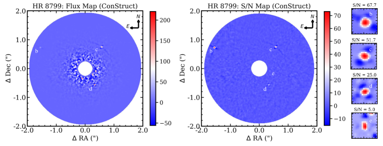
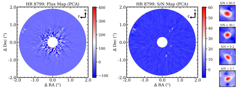
| 12 | HR 8799 b | 2012-07-22 | 133 | 3325 | 400 | Macintosh | 67.2 | 60.5 | |
| 12 | HR 8799 c | – | – | – | – | – | – | 51.7 | 30.1 |
| 12 | HR 8799 d | – | – | – | – | – | – | 25.0 | 9.2 |
| 12 | HR 8799 e | – | – | – | – | – | – | 5.0 | 3.7 |
| 13 | Gl 758 B | 2013-07-03 | 28 | 840 | 600 | Crepp | 4.2 | 10.2 | |
| 14 | Kappa And b | 2013-06-22 | 22 | 550 | 400 | Hinkley | 26.9 | 60.4 | |
| 15 | HD 4747 B | 2012-08-25 | 159 | 3816 | 300 | Johnson | 19.5 | 17.8 | |
| 16 | HD 4747 B | 2015-01-09 | 39 | 2340 | 600 | Knutson | 7.7 | 14.1 | |
| 17 | HD 8375 B | 2010-10-13 | 60 | 1086 | 300 | Crepp | 32.2 | 25.1 | |
| 18 | HD 114174 B | 2012-05-29 | 61 | 1220 | 300 | Crepp | 13.8 | 15.8 |
4 Algorithm Performance and Tuning
|
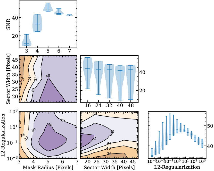
| (a) HR 8799 b |
|
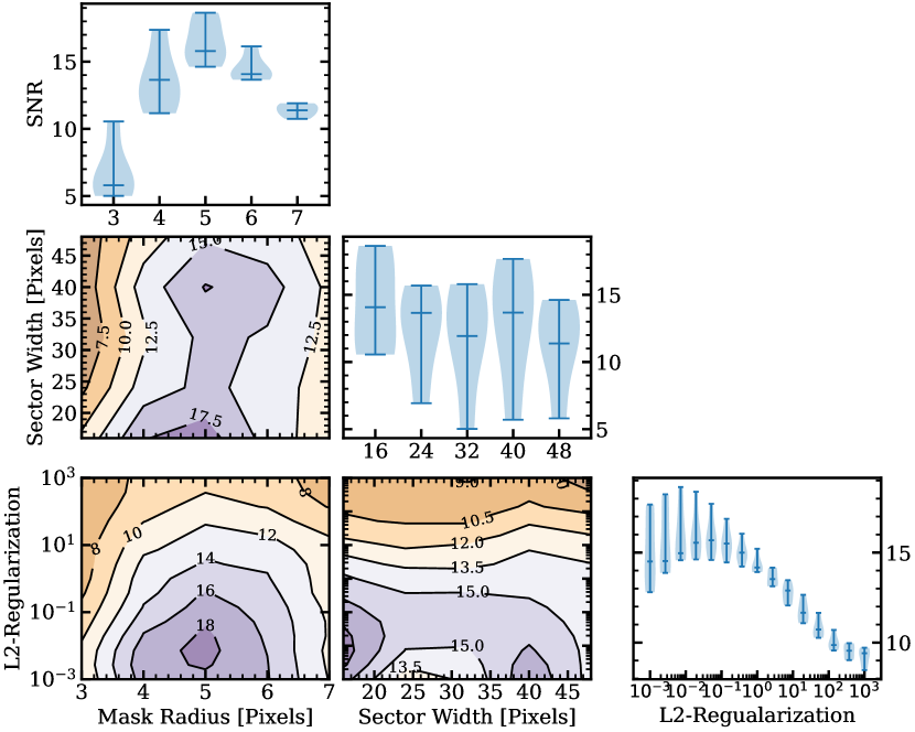
| (b) HR 8799 c |
|
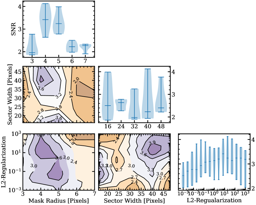
| (c) HR 8799 d |
|
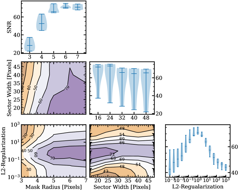
| (d) HR 8799 e |
In this section, we optimize ConStruct for detecting substellar companions in ADI sequences from NIRC2. We tune ConStruct over three selected algorithm parameters. NIRC2 ADI sequences of the HR 8799 system are used to tune our algorithm on the four known planetary companions in these data sets. This procedure allows us to select a particular parameter set for applying ConStruct on other ADI sequences. The goal is not to determine a universally optimal set of parameters, but rather to establish a reasonable set of parameter values that can then be applied to other data sets.
4.1 Selecting Design Parameters for ConStruct
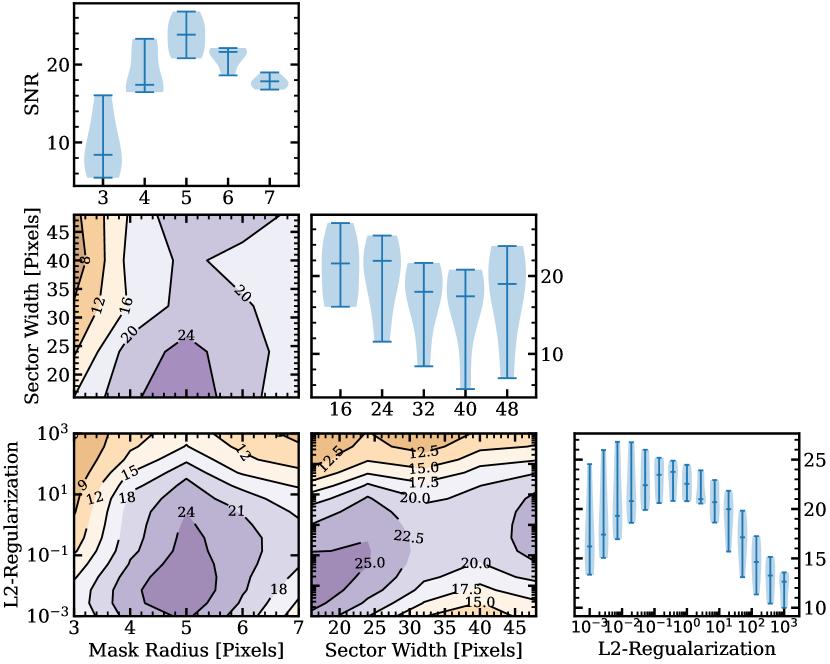
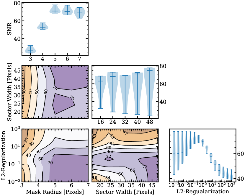
We tune three design parameters in ConStruct: 1) the radius of the masked region, , 2) the size of the sector used for the autoencoder prediction, , and 3) the regularization parameter, , in the linear correction model. Three HR 8799 ADI sequences from the Keck NIRC2 instrument serve as a test-bed for adjusting these design parameters. The objective is to find parameters that recover all four known planets in this sequence and maximize their S/N. These sequences were originally published in Konopacky et al. (2016), and the details of the observations are summarized in Table 1 in Sequences 9, 10, and 11.
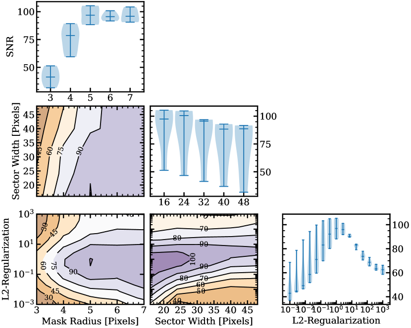
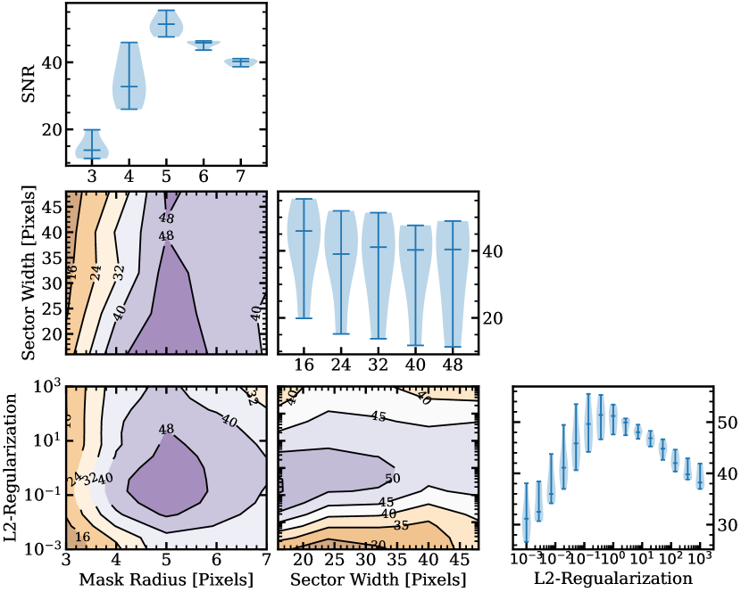
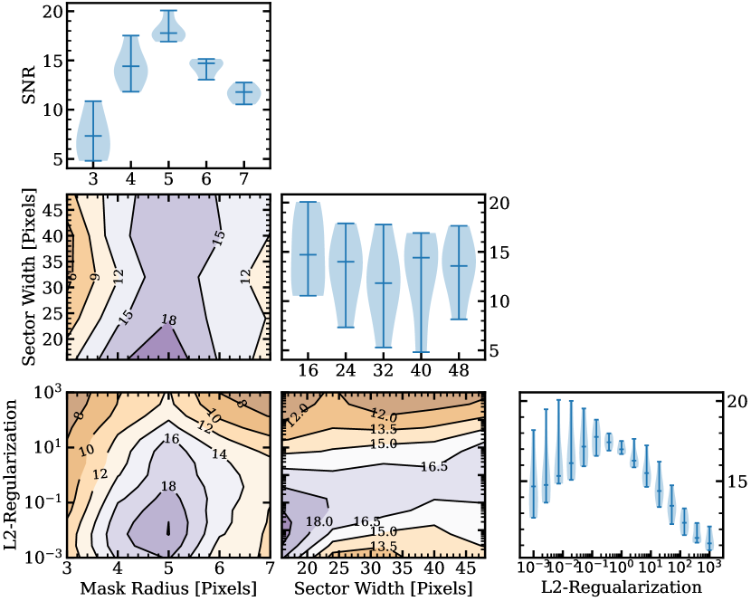
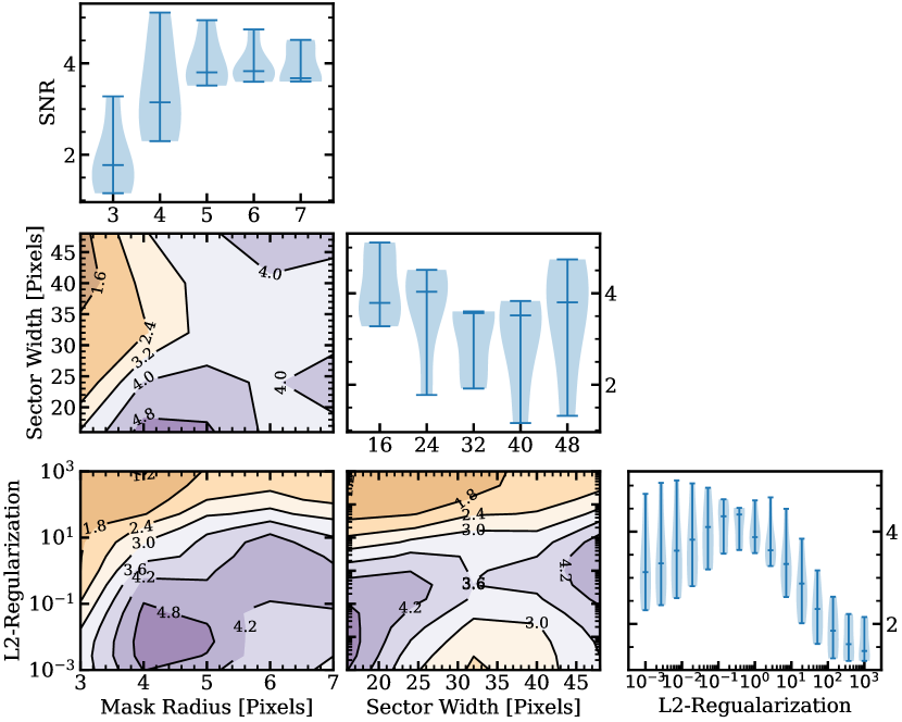
We run ConStruct over a combinatorial grid of the design parameters at the locations of the four planets for each data set. The regularization is iterated uniformly in log-space between and , with 15 increments. The mask radius is tested at values of 4, 5, 6, and 7 pixels. The radial and azimuthal widths of the image sector patches are adjusted from 16, 24, 32, and 40 pixels. In total, this produces 240 unique parameter combinations. We determine the S/N of each companion for design parameters, which creates a 3D grid with each axis corresponding to a design variable. Figure 7, show slices of the 3-D S/N grid of each planet in Sequence 10 in Table 1.
We perform the same analysis for all three HR 8799 data sets. These data have similar observation parameters (i.e., number of frames, field rotation, filter type), and we include the results for the other two sequences in Appendix D. From this study, we determine parameters that work well but are not necessarily optimal, for all planets across the three datasets in our sample. In deploying ConStruct on other datasets, we choose a sector size of 24 pixels, a mask radius of 5 pixels, and an L2 ridge regression regularization of 0.1.
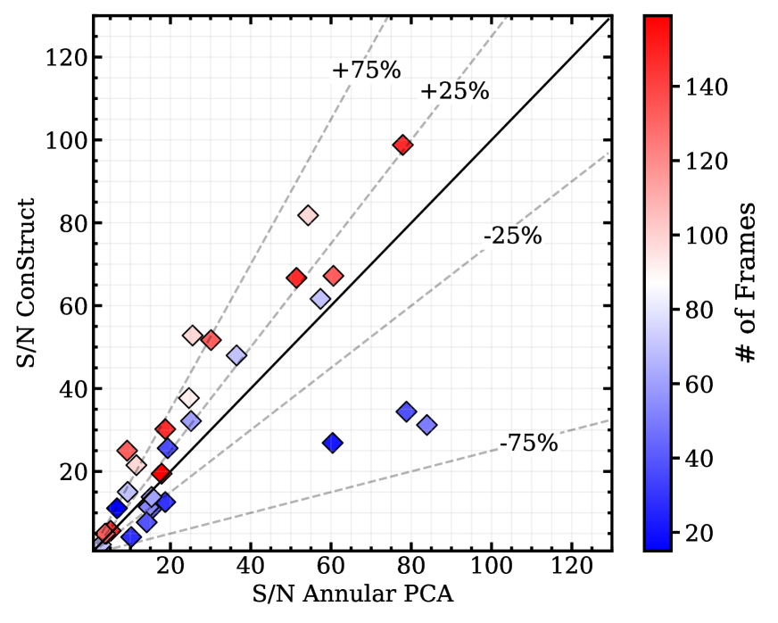
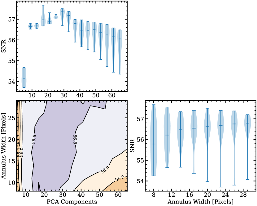
A standard annular PCA reduction serves to benchmark ConStruct’s performance on the HR 8799 ADI sequences in Table 1. For this, a similar parameter search is performed where the annular width and number of PCA components are iterated to find those that recover each of the planets at a maximal S/N. We iterate the annular width between 8 and 30 pixels in increments of 3 pixels, for a total of 7 different annular widths. The number of PCA components is iterated between 5 and the maximum allowable number, which is equivalent to the number of frames in the ADI sequence, in increments of 4 components. In Appendix E we show the performance of our PCA-based processing approach over the grid of parameters for three HR 8799 datasets contained in Table 1. Figure 8 compares these two approaches for all 12 sources in our tuning sample. For this, ConStruct produces a higher maximum S/N for planets b, c, and d than PCA over all datasets and produces comparable performance with the PCA-based reduction approach for planet e.
|
|
| (a) Maximum obtainable S/N for ConStruct and annular PCA on the tuning sample. |
|
| (b) Sample S/N for ConStruct and annular PCA. |
5 Performance on NIRC2 ADI Data
5.1 Sample S/N Comparison with PCA and ConStruct
We applied ConStruct to additional datasets obtained from KOA and compared the performance with a standard annnular PCA reduction approach. The 18 ADI sequences chosen contain known faint companions and are included in Table 1. In total, the sample includes 30 unique point sources. For all datasets, ConStruct uses the design parameters identified in Section 4. To provide a fair comparison between ConStruct and annular PCA, we also fix a set of design variables for our PCA reduction approach over this testing dataset. We identified the suitable design variables to be 17 pixels for the annulus width while using the maximum allowable number of PCA components (i.e., the number of frames in the ADI sequence).
|
| (a) ConStruct |
|
| (b) Annular PCA |
|
| (a) ConStruct |
|
| (b) Annular PCA |
|
| (a) Sequence 11 |
|
| (b) Sequence 12 |
For all the sources in our sample, we determine the recovered S/N produced from ConStruct and PCA with these fixed design parameters. Figure 8 shows a one-to-one comparison of the two algorithms for all 30 sources in our sample. ConStruct recovers 20 out of the 30 point sources at a higher S/N than PCA. Additionally, we find that the number of frames in the ADI sequence is correlated with ConStruct’s performance, where more frames give a higher S/N for ConStruct than PCA. The L2 regularization coefficient, , chosen in tuning ConStruct is likely the primary driver for this trend333For sequences with few frames, choosing a non-zero regularization prevents over-fitting. In this study, ConStruct is tuned on sequences with many frames, so the algorithm sees better results when deployed on sequences with similar characteristics..
5.2 Full Frame Reductions
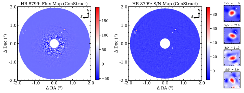
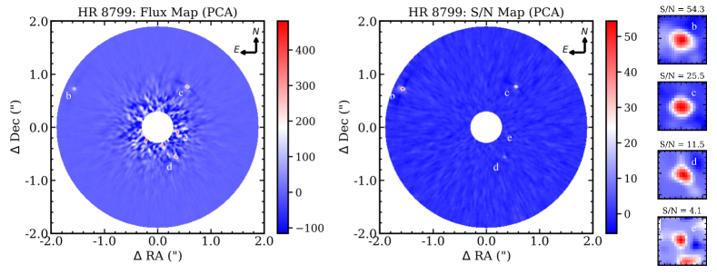
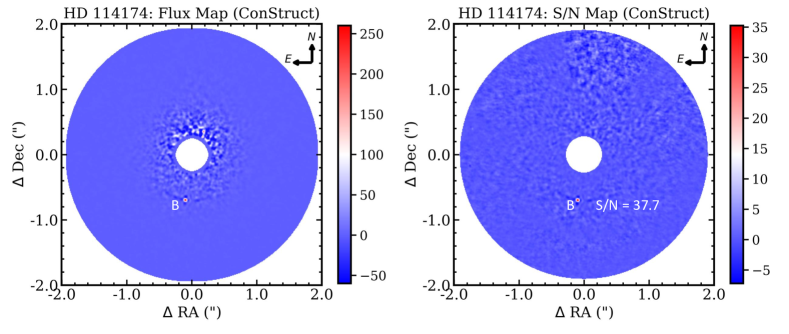
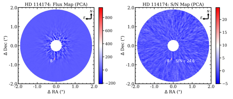
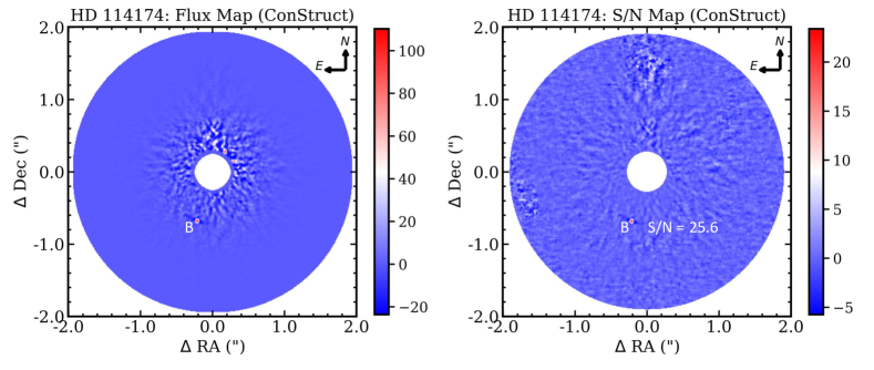
Figures 9 and 10 highlight two representative full-frame reductions for HR 8799 (Marois et al., 2008, 2010) and HD 114174 (Crepp et al., 2013) using ConStruct and PCA. The top and bottom panels correspond to the reductions produced by ConStruct and PCA, respectively. For each, the flux map (left) and S/N map (right) of the reduced data sets are shown. Each S/N map is produced by dividing the flux values in each pixel-width annulus by the empirical RMS of the residuals taken over a buffered annular region that extends pixels radially. In Figure 9, both ConStruct and PCA recover all four known planets in the HR 8799 system, however ConStruct produces a higher S/N. In Figure 10, both ConStruct and PCA recover the white dwarf companion HD 114174 B with an S/N of 37.7 and 24.6, respectively. Interestingly, individual speckle noise realizations produced by PCA appear more elongated radially whereas those produced by ConStruct have much less spatial covariance in the image plane. This effect may be attributed to the inclusion of data set diversity in training ConStruct over many ADI sequences.
5.3 Contrast Curves
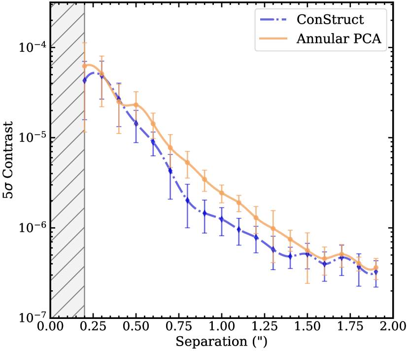
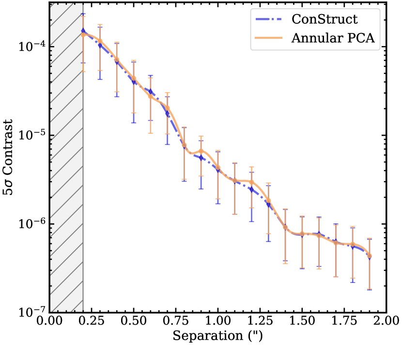
We generate contrast curves to rigorously compare the performance of ConStruct with PCA for two HR 8799 ADI sequences contained in Table 1. Synthetic sources are injected into each frame across varying radial separations. A source template is created by fitting a 2-D Gaussian profile to the central stellar PSF partially visible in the occulting disk of the coronagraph in NIRC2 images. Sources are injected over a grid of azimuthal coordinates and contrasts commensurate with the RMS of the residual speckle noise in a reduced image corresponding to the particular separation. For each frame, the grid is rotated in the negative parallactic rotation direction so that on-sky sources in the ADI sequence do not add coherently during the derotation and coaddition step. We perform a least-squares fit between the intensity of the injected source and the recovered S/N for each radial separation. We use the resulting fit to find the intensity of the source that is recovered at a confidence level, and divide it by the flux of the central stellar PSF to obtain the contrast. The stellar flux is found using frames of the unsaturated PSF taken immediately before or after the ADI sequence. The flux values in the unsaturated PSF are scaled linearly so that the exposure is equivalent to the ADI frames. We also determine an associated confidence interval for the contrast value by determining the sample standard deviation of the contrast value over the grid of azimuthally spaced source locations.
In Figure 11, we show contrast curves for two HR 8799 datasets, corresponding to Sequences 11 and 12 in Table 1. For Sequence 11, ConStruct shows improvement over PCA for nearly all separations. At its best, ConStruct improves the contrast by a factor of 2.6 at . Sequence 12, on the other hand, is nearly identical to PCA. The contrast curves share similar behavior to the results of the S/N analysis when comparing ConStruct and PCA. The properties of each dataset are the likely driver of these results, however it is difficult to directly attribute any one factor.
6 Conclusions
In this work, we introduced ConStruct, a deep learning-based algorithm for identifying faint point sources in ADI sequences. This algorithm uses an autoencoder neural network in a self-supervised training architecture to embed information from thousands of ADI image examples. The trained network is employed in a source present/absent processing framework to predict speckle noise, and recover faint signals in ADI sequences. We further augment the autoencoder neural network in ConStruct with a regularized least squares regression step to leverage temporal correlations in speckle noise across ADI frames. ConStruct is tuned using three datasets of the HR 8799 system taken with Keck/NIRC2 to identify suitable design parameters for a detailed assessment of its performance on other NIRC2 datasets. We demonstrated ConStruct with a sample of 30 point sources in 18 NIRC2 ADI sequences taken from KOA and compared the performance with a standard PCA-based reduction approach. For the examples analyzed, ConStruct improves the S/N of detections by up to and contrast up to a factor of 2.6.
There are several potential directions to improve ConStruct and make it more generally applicable for other high-contrast imaging datasets. This includes testing alternative data types for training and deploying ConStruct, including different filters and additional instruments besides NIRC2. It is also possible to assess a broader variety of learning architectures that may improve the accuracy of ConStruct. In ConStruct, we employ a regularized least-squares regression to use the temporal correlations in speckle noise across ADI frames. This step can potentially be implemented directly in the neural network with the addition of a Long Short-Term Memory (LSTM) block – a standard method in machine learning for predicting features with temporal correlations.
Additionally, there is growing interest in the high-contrast imaging community for processing procedures that operate under an inverse problem framework (Cantalloube et al., 2015; Flasseur et al., 2018, 2020). ConStruct may be adapted for these methods by representing speckle noise predictions as a continuous probability distribution, which can be achieved with a variational autoencoder. This work only considers single spectral band ADI sequences, but ConStruct can, in principle, be readily extended to multi-wavelength integral field units that take advantage of Spectral Differential Imaging (SDI) such as the Gemini Planet Imager (Macintosh et al., 2006), the Spectro-Polarimetric High-contrast Exoplanet REsearch (SPHERE) instrument (Beuzit et al., 2019), the Subaru Coronagraphic Extreme Adaptive Optics (SCExAO) instrument (Jovanovic et al., 2015), and MagAO-X (Males et al., 2018, 2020) by using higher dimensional convolutional layers. Finally, ConStruct and its future improvements present a promising approach for reducing data collected from the James Webb Space Telescope and future extreme adaptive optics ground-based facilities.
Acknowledgments
This research has made use of the Keck Observatory Archive (KOA), which is operated by the W. M. Keck Observatory and the NASA Exoplanet Science Institute (NExScI), under contract with the National Aeronautics and Space Administration. B.P.B. acknowledges support from the National Science Foundation grant AST-1909209, NASA Exoplanet Research Program grant 20-XRP202-0119, and the Alfred P. Sloan Foundation.
References
- Abadi et al. (2015) Abadi, M., Agarwal, A., Barham, P., et al. 2015. www.tensorflow.org.
- Alibert et al. (2005) Alibert, Y., Mordasini, C., Benz, W., & Winisdoerffer, C. 2005, A&A, 434, 343, doi: 10.1051/0004-6361:20042032
- Baron et al. (2019) Baron, F., Lafrenière, D., Étienne Artigau, et al. 2019, The Astronomical Journal, 158, 187, doi: 10.3847/1538-3881/ab4130
- Beuzit et al. (2019) Beuzit, J. L., Vigan, A., Mouillet, D., et al. 2019, A&A, 631, A155, doi: 10.1051/0004-6361/201935251
- Bowler (2016) Bowler, B. P. 2016, Publications of the Astronomical Society of the Pacific, 128, 102001, doi: 10.1088/1538-3873/128/968/102001
- Bowler et al. (2018) Bowler, B. P., Dupuy, T. J., Endl, M., et al. 2018, AJ, 155, 159, doi: 10.3847/1538-3881/aab2a6
- Burrows et al. (2001) Burrows, A., Hubbard, W. B., Lunine, J. I., & Liebert, J. 2001, Reviews of Modern Physics, 73, 719, doi: 10.1103/revmodphys.73.719
- Cantalloube et al. (2015) Cantalloube, F., Mouillet, D., Mugnier, L. M., et al. 2015, Astronomy & Astrophysics, 582, A89, doi: 10.1051/0004-6361/201425571
- Carson et al. (2013) Carson, J., Thalmann, C., Janson, M., et al. 2013, ApJ, 763, L32, doi: 10.1088/2041-8205/763/2/L32
- Chollet et al. (2015) Chollet, F., et al. 2015, Keras
- Craig et al. (2017) Craig, M., Crawford, S., Seifert, M., et al. 2017, astropy/ccdproc: v1.3.0.post1, doi: 10.5281/zenodo.1069648
- Crepp et al. (2016) Crepp, J. R., Gonzales, E. J., Bechter, E. B., et al. 2016, The Astrophysical Journal, 831, 136, doi: 10.3847/0004-637x/831/2/136
- Crepp et al. (2014) Crepp, J. R., Johnson, J. A., Howard, A. W., et al. 2014, ApJ, 781, 29, doi: 10.1088/0004-637X/781/1/29
- Crepp et al. (2013) —. 2013, ApJ, 774, 1, doi: 10.1088/0004-637X/774/1/1
- Crepp et al. (2012) Crepp, J. R., Johnson, J. A., Fischer, D. A., et al. 2012, ApJ, 751, 97, doi: 10.1088/0004-637X/751/2/97
- Crepp et al. (2013) Crepp, J. R., Johnson, J. A., Howard, A. W., et al. 2013, The Astrophysical Journal, 771, 46, doi: 10.1088/0004-637X/771/1/46
- Elharrouss et al. (2019) Elharrouss, O., Almaadeed, N., Al-Maadeed, S., & Akbari, Y. 2019, Neural Processing Letters, 51, 2007, doi: 10.1007/s11063-019-10163-0
- Fitzgerald & Graham (2005) Fitzgerald, M. P., & Graham, J. R. 2005, ApJ, 637, 541, doi: 10.1086/498339
- Flasseur et al. (2023) Flasseur, O., Bodrito, T., Mairal, J., et al. 2023, deep PACO: Combining statistical models with deep learning for exoplanet detection and characterization in direct imaging at high contrast, arXiv, doi: 10.48550/ARXIV.2303.02461
- Flasseur et al. (2018) Flasseur, O., Denis, L., Thiébaut, É., & Langlois, M. 2018, A&A, 618, A138, doi: 10.1051/0004-6361/201832745
- Flasseur et al. (2020) Flasseur, O., Denis, L., Thiébaut, E., & Langlois, M. 2020, A&A, 637, A9, doi: 10.1051/0004-6361/201937239
- Gaudi et al. (2021) Gaudi, B. S., Meyer, M., & Christiansen, J. 2021, in ExoFrontiers; Big Questions in Exoplanetary Science, ed. N. Madhusudhan, 2–1, doi: 10.1088/2514-3433/abfa8fch2
- Gebhard et al. (2022) Gebhard, T. D., Bonse, M. J., Quanz, S. P., & Schölkopf, B. 2022, Half-sibling regression meets exoplanet imaging: PSF modeling and subtraction using a flexible, domain knowledge-driven, causal framework, arXiv, doi: 10.48550/ARXIV.2204.03439
- Gonzalez et al. (2018) Gonzalez, C. A. G., Absil, O., & Droogenbroeck, M. V. 2018, Astronomy & Astrophysics, 613, A71, doi: 10.1051/0004-6361/201731961
- Guyon (2005) Guyon, O. 2005, The Astrophysical Journal, 629, 592, doi: 10.1086/431209
- Guyon et al. (2006) Guyon, O., Pluzhnik, E. A., Kuchner, M. J., Collins, B., & Ridgway, S. T. 2006, The Astrophysical Journal Supplement Series, 167, 81, doi: 10.1086/507630
- Hastie et al. (2009) Hastie, T., Tibshirani, R., & Friedman, J. 2009, The Elements of Statistical Learning, 2nd edn. (Springer). /bib/hastie/Hastie2001/ESLII_print10.pdf,http://www-stat.stanford.edu/~tibs/ElemStatLearn/,/bib/hastie/Hastie2001/weatherwax_epstein_hastie_solutions_manual.pdf
- Hinkley et al. (2007) Hinkley, S., Oppenheimer, B. R., Soummer, R., et al. 2007, ApJ, 654, 633, doi: 10.1086/509063
- Jovanovic et al. (2015) Jovanovic, N., Martinache, F., Guyon, O., et al. 2015, Publications of the Astronomical Society of the Pacific, 127, 890, doi: 10.1086/682989
- Kingma & Ba (2015) Kingma, D. P., & Ba, J. 2015, in 3rd International Conference on Learning Representations, ICLR 2015, San Diego, CA, USA, May 7-9, 2015, Conference Track Proceedings, ed. Y. Bengio & Y. LeCun. http://arxiv.org/abs/1412.6980
- Konopacky et al. (2016) Konopacky, Q. M., Marois, C., Macintosh, B. A., et al. 2016, The Astronomical Journal, 152, doi: 10.3847/0004-6256/152/2/28
- Lafrenière et al. (2009) Lafrenière, D., Marois, C., Doyon, R., & Barman, T. 2009, ApJ, 694, L148, doi: 10.1088/0004-637X/694/2/L148
- Lafreniere et al. (2007) Lafreniere, D., Marois, C., Doyon, R., Nadeau, D., & Artigau, E. 2007, The Astrophysical Journal, 660, 770, doi: 10.1086/513180
- Liu (2004) Liu, M. C. 2004, Science, 305, 1442, doi: 10.1126/science.1102929
- Liu et al. (2002) Liu, M. C., Fischer, D. A., Graham, J. R., et al. 2002, ApJ, 571, 519, doi: 10.1086/339845
- Lovis et al. (2010) Lovis, C., Fischer, D., Lovis, C., & Fischer, D. 2010, exop, 27. https://ui.adsabs.harvard.edu/abs/2010exop.book...27L/abstract
- Macintosh et al. (2006) Macintosh, B., Graham, J., Palmer, D., et al. 2006, in Advances in Adaptive Optics II, ed. B. L. Ellerbroek & D. B. Calia, Vol. 6272, International Society for Optics and Photonics (SPIE), 62720L, doi: 10.1117/12.672430
- Males et al. (2018) Males, J. R., Close, L. M., Miller, K., et al. 2018, in Society of Photo-Optical Instrumentation Engineers (SPIE) Conference Series, Vol. 10703, Adaptive Optics Systems VI, ed. L. M. Close, L. Schreiber, & D. Schmidt, 1070309, doi: 10.1117/12.2312992
- Males et al. (2020) Males, J. R., Close, L. M., Guyon, O., et al. 2020, in Society of Photo-Optical Instrumentation Engineers (SPIE) Conference Series, Vol. 11448, Society of Photo-Optical Instrumentation Engineers (SPIE) Conference Series, 114484L, doi: 10.1117/12.2561682
- Marois et al. (2005) Marois, C., Lafreniere, D., Doyon, R., Macintosh, B., & Nadeau, D. 2005, The Astrophysical Journal, 641, 556, doi: 10.1086/500401
- Marois et al. (2008) Marois, C., Macintosh, B., Barman, T., et al. 2008, Science, 322, 1348, doi: 10.1126/science.1166585
- Marois et al. (2010) Marois, C., Zuckerman, B., Konopacky, Q. M., Macintosh, B., & Barman, T. 2010, Nature, 468, 1080, doi: 10.1038/nature09684
- Martinez et al. (2012) Martinez, P., Loose, C., Aller Carpentier, E., & Kasper, M. 2012, A&A, 541, A136, doi: 10.1051/0004-6361/201118459
- Mawet et al. (2014) Mawet, D., Milli, J., Wahhaj, Z., et al. 2014, ApJ, 792, 97, doi: 10.1088/0004-637X/792/2/97
- Nielsen et al. (2019) Nielsen, E. L., De Rosa, R. J., Macintosh, B., et al. 2019, VizieR Online Data Catalog, J/AJ/158/13
- Oppenheimer & Hinkley (2009) Oppenheimer, B. R., & Hinkley, S. 2009, Annual Review of Astronomy and Astrophysics, 47, 253, doi: 10.1146/annurev-astro-082708-101717
- Pueyo et al. (2012) Pueyo, L., Crepp, J. R., Vasisht, G., et al. 2012, The Astrophysical Journal Supplement Series, 199, 6, doi: 10.1088/0067-0049/199/1/6
- Ronneberger et al. (2015) Ronneberger, O., Fischer, P., & Brox, T. 2015, U-Net: Convolutional Networks for Biomedical Image Segmentation, arXiv, doi: 10.48550/ARXIV.1505.04597
- Sanghi et al. (2022) Sanghi, A., Zhou, Y., & Bowler, B. P. 2022, AJ, 163, 119, doi: 10.3847/1538-3881/ac477e
- Seager (2008) Seager, S. 2008, Space Science Reviews 2008 135:1, 135, 345, doi: 10.1007/S11214-008-9308-5
- Soummer et al. (2012) Soummer, R., Pueyo, L., & Larkin, J. 2012, Astrophysical Journal Letters, 755, doi: 10.1088/2041-8205/755/2/L28
- Sparks & Ford (2002) Sparks, W. B., & Ford, H. C. 2002, The Astrophysical Journal, 578, 543, doi: 10.1086/342401
- Vigan et al. (2021) Vigan, A., Fontanive, C., Meyer, M., et al. 2021, A&A, 651, A72, doi: 10.1051/0004-6361/202038107
- Wahhaj et al. (2021) Wahhaj, Z., Milli, J., Romero, C., et al. 2021, A&A, 648, A26, doi: 10.1051/0004-6361/202038794
- Xie et al. (2022) Xie, C., Choquet, E., Vigan, A., et al. 2022, arXiv e-prints, arXiv:2208.07915. https://arxiv.org/abs/2208.07915
- Yip et al. (2019) Yip, K. H., Nikolaou, N., Coronica, P., et al. 2019, Lecture Notes in Computer Science (including subseries Lecture Notes in Artificial Intelligence and Lecture Notes in Bioinformatics), 11908 LNAI, 322, doi: 10.1007/978-3-030-46133-1_20
Appendix A Autoencoder Architecture
Here we show the parameters for the autoencoder neural network used in ConStruct. In total, the autoencoder consists of 32 unique layers. In Table 2, we show the parameters for each layer in the network, which include the layer type and the size of the layer.
| Layer | Type | Tensor Size |
|---|---|---|
| 0 | Input | (32, 32, 1) |
| 1 | Conv. | (32, 32, 32) |
| 2 | Conv. | (32, 32, 32) |
| 3 | Max. Pool | (16, 16, 32) |
| 4 | Conv. | (16, 16, 64) |
| 5 | Conv. | (16, 16, 64) |
| 6 | Max. Pool | (8, 8, 64) |
| 7 | Conv. | (8, 8, 128) |
| 8 | Conv. | (8, 8, 128) |
| 9 | Max. Pool | (4, 4, 128) |
| 10 | Conv. | (4, 4, 256) |
| 11 | Conv. | (4, 4, 256) |
| 12 | Max. Pool | (2, 2, 256) |
| 13 | Conv. | (2, 2, 512) |
| 14 | Conv. | (2, 2, 512) |
| 15 | Up Conv. | (4, 4, 256) |
| 16 | Concatenate | (4, 4, 512) |
| 17 | Conv. | (4, 4, 256) |
| 18 | Conv. | (4, 4, 256) |
| 19 | Up Conv. | (8, 8, 128) |
| 20 | Concatenate | (8, 8, 256) |
| 21 | Conv. | (8, 8, 128) |
| 22 | Conv. | (8, 8, 128) |
| 23 | Up Conv. | (16, 16, 64) |
| 24 | Concatenate | (16, 16, 128) |
| 25 | Conv. | (16, 16, 64) |
| 26 | Conv. | (16, 16, 64) |
| 27 | Up Conv. | (32, 32, 32) |
| 28 | Concatenate | (32, 32, 64) |
| 29 | Conv. | (32, 32, 32) |
| 30 | Conv. | (32, 32, 32) |
| 31 | Output | (32, 32, 1) |
Appendix B Additional Autoencoder Predictions of Speckle Noise
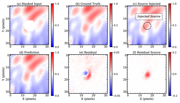
Here we show two additional examples demonstrating how the autoencoder neural network can predict the speckle noise in an image patch extracted from an ADI sequence. In this example, the patches are extracted from a frame contained in an ADI seqeunce of the HR 8799 system, corresponding to Sequence 9 in Table 1. A synthetic 2-D Gaussian source is injected into the center of the the image patch. The central region is then masked before being fed into the network.
|
| (a) |
|
| (b) |
Appendix C Training Data
In Table 3, we include the ADI sequences used for training ConStruct. These data are obtained from KOA. In total, 92 unique ADI sequences are used from various targets, many with known companions.
| Target | Date (UT) | # of Frames | Int. Time (s) | Filter | Program PI |
|---|---|---|---|---|---|
| GJ 504 | 2002-06-15 | 20 | 1200 | Charbonneau | |
| HN Peg | 2002-06-15 | 20 | 1200 | Charbonneau | |
| HR 6070 | 2003-03-13 | 15 | 435.6 | Liu | |
| 51 Eri | 2003-03-13 | 15 | 435.6 | Liu | |
| GI 355 | 2003-03-14 | 15 | 435.6 | Liu | |
| V889 Her | 2003-06-18 | 10 | 300 | Liu | |
| 49 Seti | 2003-11-11 | 10 | 600 | Liu | |
| HD 25457 | 2003-11-11 | 10 | 435.6 | Liu | |
| HD 22049 | 2003-11-11 | 10 | 435.6 | Liu | |
| HD 22049 | 2003-12-07 | 9 | 540 | de Pater | |
| HR 4796 | 2003-12-07 | 21 | 210 | Kalas | |
| HR 4796 | 2003-12-07 | 11 | 330 | Kalas | |
| HIP 102409 | 2004-05-30 | 48 | 2400 | dePater | |
| HIP 6276 | 2004-09-08 | 15 | 450 | Liu | |
| HD 147513 | 2005-04-18 | 14 | 840 | Kalas | |
| V889 Her | 2005-07-15 | 10 | 290.4 | Liu | |
| HD 191089 | 2005-10-21 | 15 | 300 | Kalas | |
| HIP 17395 | 2008-11-04 | 95 | 1900 | Macintosh | |
| HD 92945 | 2008-12-03 | 40 | 1600 | Kalas | |
| HD 107146 | 2008-12-17 | 55 | 880 | Jayawardhana | |
| HD 161868 | 2009-04-13 | 35 | 525 | Law | |
| HD 984 | 2009-07-31 | 60 | 1200 | Macintosh | |
| HIP 1134 | 2009-08-07 | 90 | 1800 | Macintosh | |
| HIP 7345 | 2009-08-07 | 107 | 2140 | Macintosh | |
| HIP 91043 | 2009-08-07 | 88 | 1760 | Macintosh | |
| HIP 95793 | 2009-11-01 | 60 | 2400 | Macintosh | |
| HIP 21547 | 2009-11-02 | 33 | 1980 | Macintosh | |
| HD 61005 | 2009-11-24 | 205 | 1025 | Kalas | |
| HD 61005 | 2009-12-05 | 58 | 1740 | Kalas | |
| HD 131835 | 2010-04-03 | 13 | 390 | Fitzgerald | |
| HD 131835 | 2010-04-03 | 92 | 2208 | Fitzgerald | |
| HD 131835 | 2010-04-03 | 109 | 3270 | Fitzgerald | |
| GL 758 | 2010-05-02 | 102 | 3060 | Biller | |
| HIP 95793 | 2010-07-10 | 45 | 1350 | Macintosh | |
| HIP 76063 | 2010-07-11 | 40 | 1200 | Macintosh | |
| HIP 95347 | 2010-07-11 | 56 | 1680 | Macintosh | |
| HIP 72197 | 2010-07-12 | 45 | 1350 | Macintosh | |
| HD 10008 | 2010-09-26 | 70 | 1680 | Hinkley | |
| HD 8375 | 2010-10-13 | 60 | 1086 | Crepp | |
| HIP 53954 | 2011-02-06 | 100 | 145.2 | Hinkley | |
| HIP 53954 | 2011-02-06 | 20 | 290.4 | Hinkley | |
| HIP 24528 | 2011-02-06 | 60 | 2400 | Hinkley | |
| HIP 25453 | 2011-02-06 | 60 | 960 | Hinkley | |
| HD 114174 | 2011-02-22 | 37 | 740 | Crepp | |
| HR 7672 | 2011-05-15 | 15 | 30 | Carpenter | |
| HR 7672 | 2011-05-15 | 30 | 450 | Carpenter | |
| HD 206860 | 2011-07-17 | 60 | 304.9 | Morales | |
| HD 206860 | 2011-07-17 | 41 | 208.4 | Morales | |
| HD 19467 | 2011-08-30 | 50 | 1250 | Crepp | |
| HD 61005 | 2012-01-04 | 21 | 420 | Fitzgerald | |
| HD 61005 | 2012-01-04 | 21 | 420 | Fitzgerald | |
| HD 61005 | 2012-01-04 | 61 | 1830 | Fitzgerald | |
| HD 114174 | 2012-02-02 | 92 | 1840 | Knutson | |
| HD 114174 | 2012-02-02 | 92 | 1840 | Knutson | |
| HD 114174 | 2012-05-29 | 10 | 250 | Crepp | |
| HD 114174 | 2012-05-29 | 61 | 1220 | Crepp | |
| HD 114174 | 2012-06-24 | 51 | 1275 | Crepp | |
| HD 114174 | 2012-07-04 | 100 | 2400 | Johnson | |
| HIP 107350 | 2012-07-22 | 30 | 600 | Macintosh | |
| HD 4747 | 2012-08-25 | 159 | 3816 | Johnson | |
| HD 19467 | 2012-08-26 | 20 | 600 | Crepp | |
| HD 19467 | 2012-08-26 | 20 | 480 | Crepp | |
| HIP 21547 | 2012-09-04 | 52 | 1560 | Macintosh | |
| HD 206860 | 2012-10-27 | 60 | 300 | Morales | |
| HIP 6276 | 2012-10-27 | 40 | 1400 | Morales | |
| HIP 44526 | 2012-12-05 | 23 | 920 | Hinkley | |
| Kappa And | 2013-05-01 | 43 | 778.3 | Hinkley | |
| HIP 116805 | 2013-05-30 | 38 | 1520 | Carpenter | |
| HIP 116805 | 2013-06-22 | 22 | 550 | Hinkley | |
| HD 182488 | 2013-07-03 | 28 | 840 | Crepp | |
| HIP 116805 | 2013-08-18 | 15 | 300 | Johnson | |
| HIP 11152 | 2013-09-25 | 58 | 290 | Hinkley | |
| HIP 45950 | 2014-01-12 | 48 | 720 | Knutson | |
| GJ 504 | 2014-05-13 | 30 | 150 | Hinkley | |
| GJ 504 | 2014-05-13 | 68 | 680 | Hinkley | |
| HD 114174 | 2014-05-21 | 10 | 100 | Knutson | |
| HD 114174 | 2014-05-21 | 10 | 100 | Knutson | |
| HD 4747 | 2014-10-12 | 201 | 6030 | Crepp | |
| HD 203030 | 2014-11-09 | 60 | 1800 | Bowler | |
| HD 4747 | 2015-01-09 | 39 | 2340 | Knutson | |
| HD 35841 | 2015-01-10 | 72 | 2880 | Hinkley | |
| HN Peg | 2015-06-02 | 71 | 2130 | Knutson | |
| HD 203030 | 2015-06-03 | 105 | 3150 | Knutson | |
| HIP 60074 | 2015-06-06 | 172 | 344 | Padgett | |
| GJ 504 | 2015-06-08 | 91 | 2730 | Currie | |
| Kappa And | 2016-05-26 | 29 | 580 | Mawet | |
| HD 191089 | 2016-06-26 | 144 | 4180.3 | Kalas | |
| K12 | 2016-08-20 | 100 | 400 | Morales | |
| HD 43989 | 2017-11-16 | 70 | 2240 | Choquet | |
| Kappa And | 2017-12-10 | 10 | 300 | Currie | |
| Kappa And | 2018-01-30 | 15 | 450 | Bowler | |
| Gamma Cep | 2019-07-07 | 20 | 106 | Bowler |
Appendix D Tuning ConStruct with the HR 8799 Planets
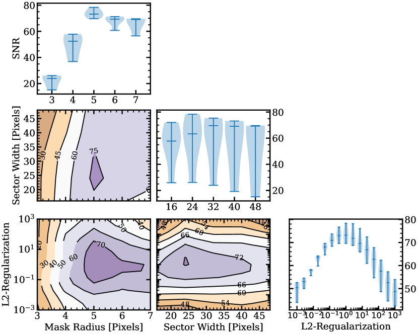
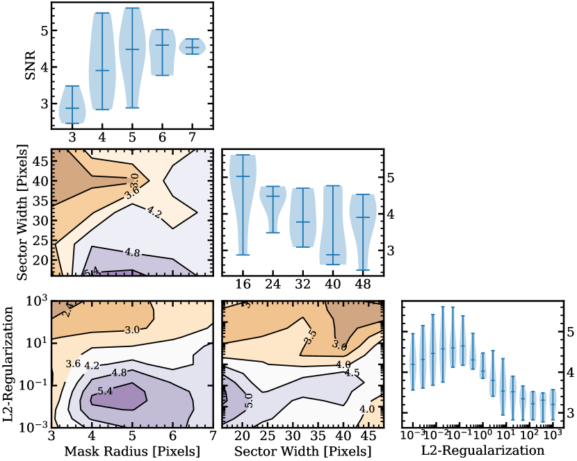
Here, we show the additional marginalized representations of the 3-D S/N parameter search, used for tuning ConStruct. Figure 13 shows the representation for Sequence 9 in Table 1. Figure 14 shows the marginalized representation for Sequence 10.
|
| (a) HR 8799 b |
|
| (b) HR 8799 c |
|
| (c) HR 8799 d |
|
| (d) HR 8799 e |
|
| (a) HR 8799 b |
|
| (b) HR 8799 c |
|
| (c) HR 8799 d |
|
| (d) HR 8799 e |
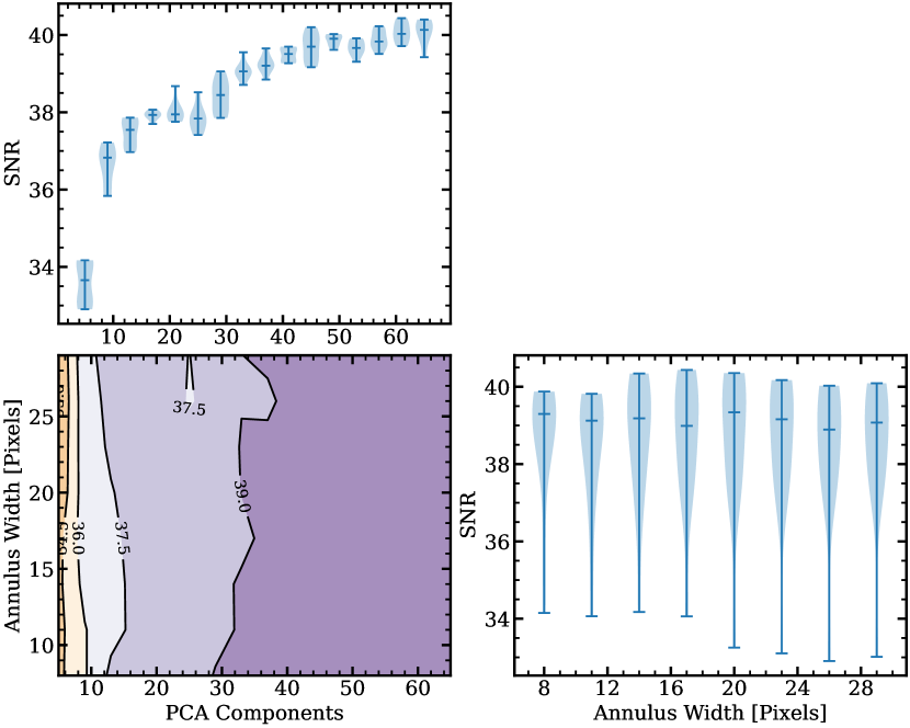
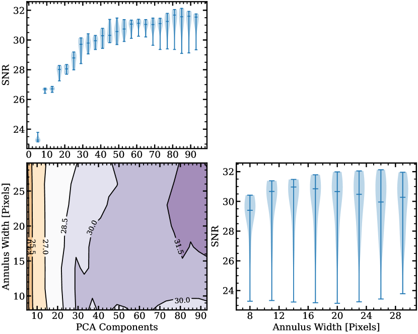
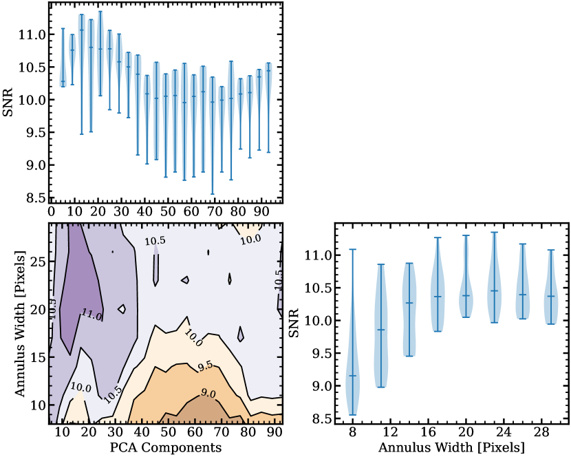
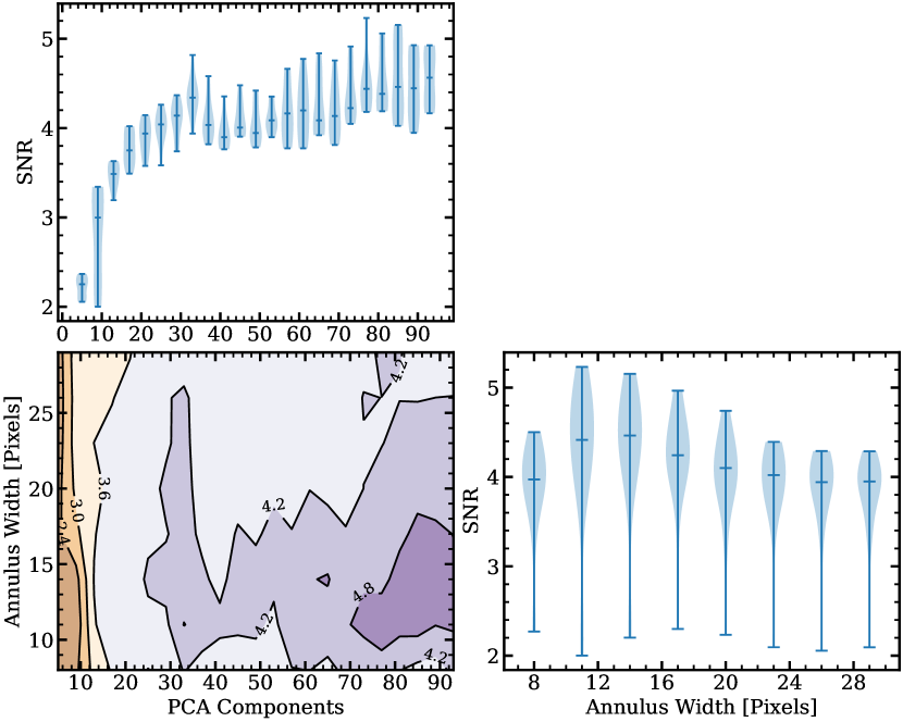
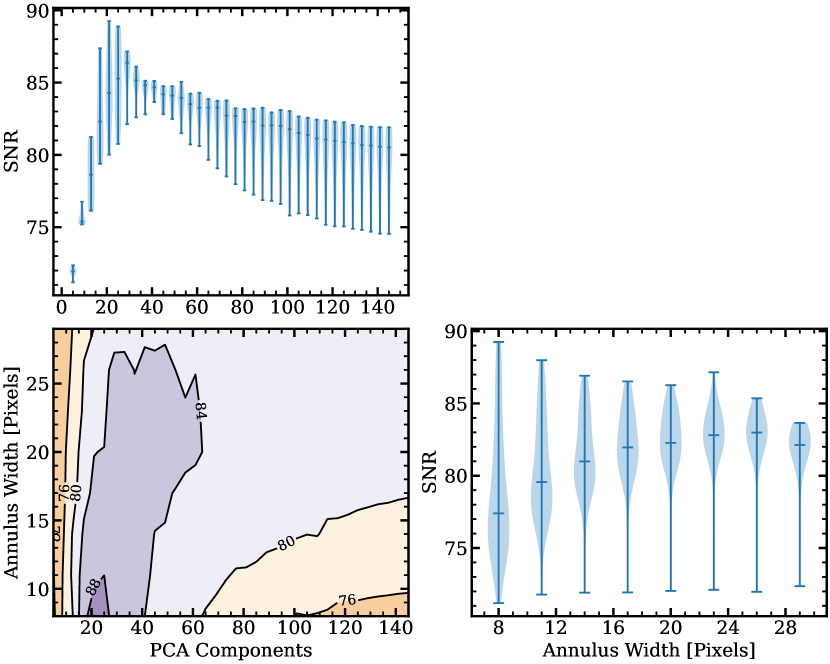
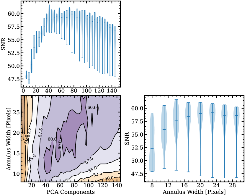
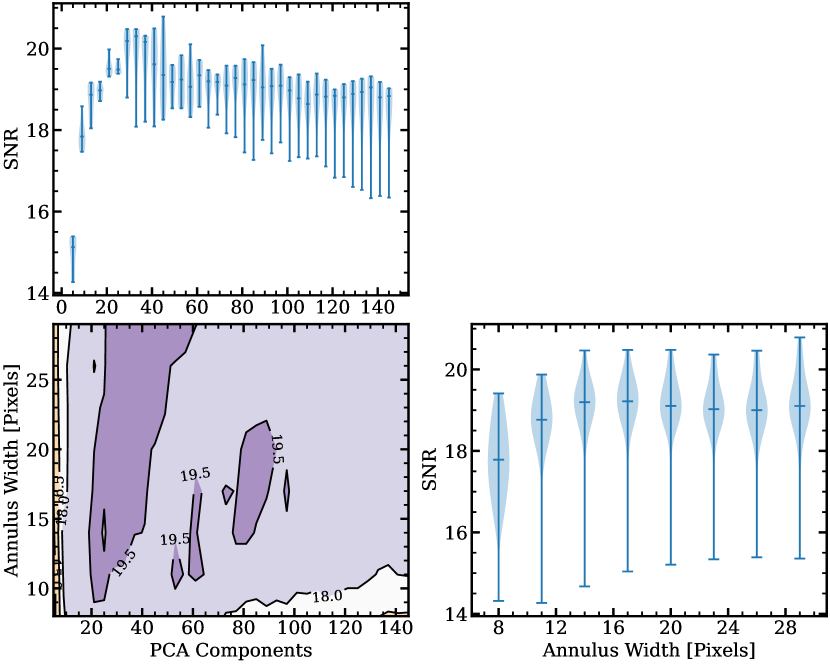
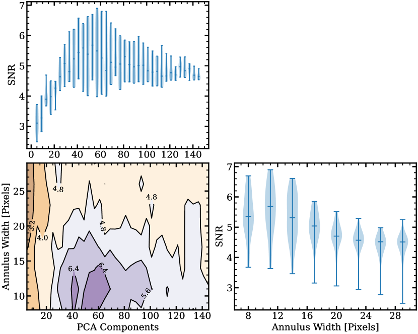
Appendix E Tuning PCA reductions with the HR 8799 Planets
Here, we show the performance of PCA post-processing over a grid of parameters tested on the HR 8799 planets. The grid is generated over a range of PCA components and annulus widths. The PCA components are sampled in increments of four components, starting at five, and terminating at the maximum allowable components (i.e., number of frames in the ADI sequence). The grid samples annulus widths in increments of three pixels, starting at 8 pixels and ending at 30.
|
| (a) HR 8799 b |
|
| (b) HR 8799 c |
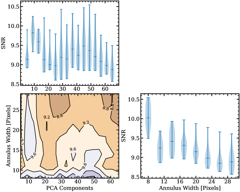
|
| (c) HR 8799 d |
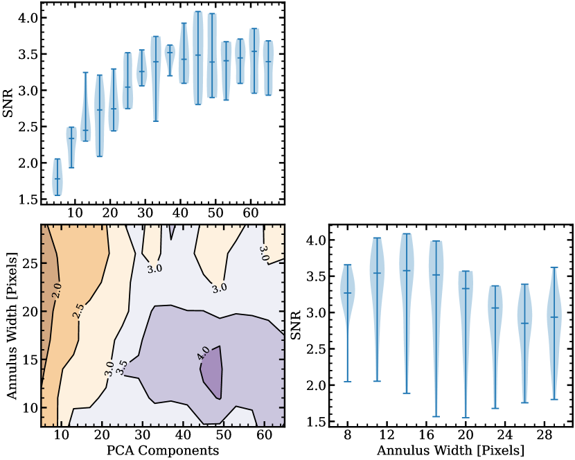
|
| (d) HR 8799 e |
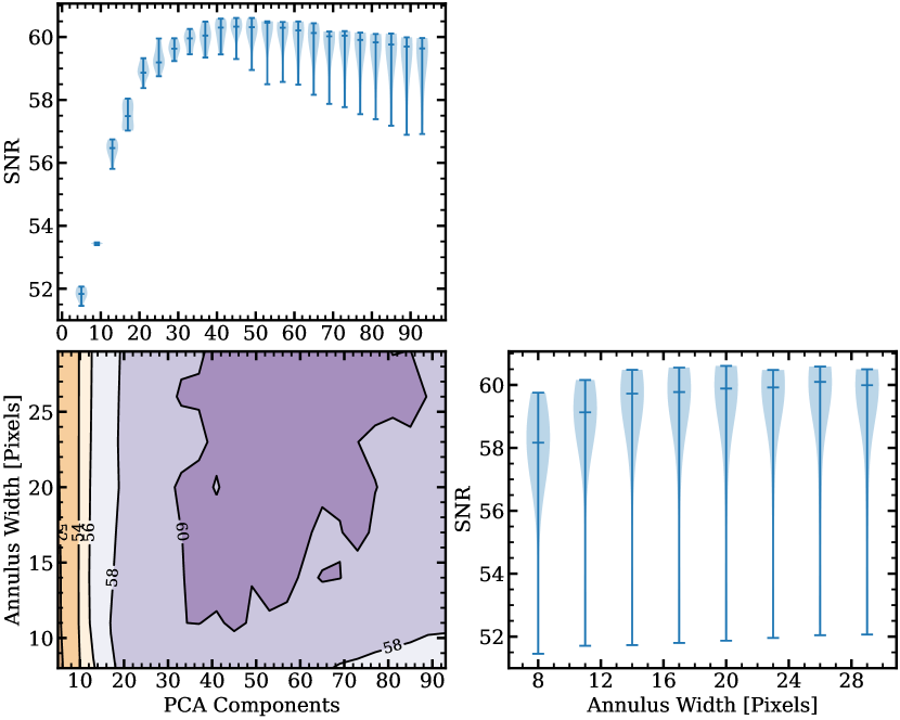
|
| (a) HR 8799 b |
|
| (b) HR 8799 c |
|
| (c) HR 8799 d |
|
| (d) HR 8799 e |
|
| (a) HR 8799 b |
|
| (b) HR 8799 c |
|
| (c) HR 8799 d |
|
| (d) HR 8799 e |
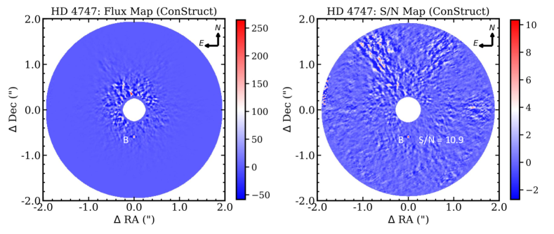
Appendix F Additional Reductions
Here, we show additional full-frame reductions of the ADI datasets used in this study processed with both ConStruct and PCA. Figure 18 shows the reductions for HD 4747 (Crepp et al., 2016), corresponding to Sequence 1 in Table 1. Figure 19 shows HD 19467 (Crepp et al., 2014) for Sequence 2. Figure 20 is for HD 114174 (Crepp et al., 2013), corresponding to Sequence 4. Figure 21 is for HR 7672 (Liu et al., 2002), corresponding to Sequence 7. Figures 22 and 23 show two Kappa And (Carson et al., 2013) reductions corresponding to Sequences 8 and 9, respectively. Figures 24 and 25 show two HR 8799 (Marois et al., 2008, 2010) reductions corresponding to Sequences 10 and 11, respectively.
|
| (a) ConStruct |
|
| (b) Annular PCA |
|
| (a) ConStruct |
|
| (b) Annular PCA |
|
| (a) ConStruct |
|
| (b) Annular PCA |
|
| (a) ConStruct |
|
| (b) Annular PCA |
|
| (a) ConStruct |
|
| (b) Annular PCA |
|
| (a) ConStruct |
|
| (b) Annular PCA |