Impact of carbon market on production emissions
Abstract
The aim of this paper is to address the effect of the carbon emission allowance market on the production policy of a large polluter production firm. We investigate this effect in two cases; when the large polluter cannot affect the risk premium of the allowance market, and when it can change the risk premium by its production. In this simple model, we ignore any possible investment of the firm in pollution reducing technologies. We formulate the problem of optimal production by a stochastic optimization problem. Then, we show that, as expected, the market reduces the optimal production policy in the first case if the firm is not given a generous initial cheap allowance package. However, when the large producer activities can change the market risk premium, the cut on the production and consequently pollution cannot be guaranteed. In fact, there are cases in this model when the optimal production is always larger than expected, and an increase in production, and thus pollution, can increase the profit of the firm. We conclude that some of the parameters of the market which contribute to this effect can be wisely controlled by the regulators in order to diminish this manipulative behavior of the firm.
Key words: EU ETS, Carbon emission allowance, Optimal production policy, HJB equations
AMS 2000 subject classifications: 91G80, 93E20, 91B70.
1 Introduction
The long term costs of global warming is believed to be significantly more than the cost of controlling it by reducing the pollution due to greenhouse gases (see [13]). The Kyoto protocol in 1997 concerns with the reduction of the greenhouse gases including and is accepted by several nations. These nations agreed to set goal on reduction of greenhouse gases and implement plans to reach the goals. One of the popular plans in the so-called cap-and-trade scheme adopted by several nations including members of European Union. The principle behind standard cap-and-trade is simple. Regulator marks the polluter installations and set a cap on the total emission at the end of a specific period of time and issue a number of allowances equal to the cap. Then, they allocate the allowances to the those installations. If the cap is reached, then all installations are mandated to pay a predetermined penalty or present sufficient allowances. At the same time, there is a market where they can trade for the allowances; if a firm does not need its allowances for whatever reason, they can sell it to those who want to produce more. Ther allowance papers are worthless, if the cap is not reached.
There are several variations of standard cap-and-trade scheme, running around the world, e.g. European Union Emission Trading Scheme (EU ETS), US REgenial CLean Air Incentive Market (RECLAIM) or Regional Greenhouse Gas Incentive (RGGI). Although based on the same principle, they may differ in certain details. Some of the specifics of the cap-and-trade market is to make it work more efficiently. For instance to avoid a sharp drop in the allowance price when the cap is not reachable, they can store their allowances for the next period of the scheme by paying an extra fee per allowance, which is referred to as banking. Also, regulator can distribute initial allowances to involved installations for free, or they can set an auction to distribute them, or a mixture of both. For example in the third phase of EU ETS 2013-2020, 40% of the allowances are distributed by auctioning, while in the first two phases 2006-2008 and 2008-2012, the allowances are distributed for free. Also, the cap can be set regionally where each region has its own cap on the total emission of the region, or globally where all regions have one cap on the total emission. The later creates a less stressful market. The efficiency of the design of the market is comprehensively studied in [5] where they show in the standard cap-and-trade system the presence of windfall profit based on the real market data and propose a more efficient allocation scheme. In [4], the authors study some alternatives to the standard cap-and-trade system which can potentially lead to less windfall profit for a dominant player in the market and less cost for the consumers of the product of the polluter firms. More precisely, in addition to initial auctioning, they propose to allocate part of the allowance over time, which make it more flexible for the regulator to achieve its pollution reduction target with less cost on the economy.
Several studies target the dynamics of the price of the allowance. In the presence of banking, the price of allowance in the current period can be viewed as an option on the price of allowance for the next period (See for example [6]). This approach is obviously not capable of explaining the price of the most farthest period, and therefore, it is important to take a different approach to explain the dynamics for the price in the last period. In [3], by adopting a stochastic game setting in discrete-time, the authors show the existence of a Nash equilibrium for the price of emission allowance, which appears to be a martingale. In addition, they show that this equilibrium price is equal to the marginal cost of total abatement which can be obtained by solving the problem of minimizing the total abatement cost in the market. In [2], they study the formation of equilibrium price in a continuous-time setting through a system of forward-backward SDEs (FBSDE) with singularity at terminal time. In their study, the singularity of the terminal condition is two-folded; one caused by the discontinuity of terminal condition of backward equation and the other by the degeneracy of the forward equation at terminal time. Then for some specific pathological examples, they showed the existence and the uniqueness of the solution to the system of FBSDEs, by approximating the terminal condition with smooth functions in a certain manner. Beside modeling allowance price by FBSDE, their main contribution is to bold the difficulties caused by discontinuous terminal condition of backward component and the demand for a more inclusive theory of FBSDEs in this case.
In this paper, we analyze the effect of the cap-and-trade scheme in reducing the carbon emission through reduction on the optimal production of the relevant production firms. The setting of this paper is similar to the third phase of EU ETS where one EU-wide cap on total emission is imposed. The firm’s objective is to maximize its utility on wealth, which is made of the profit gained from production and the value of carbon allowance portfolio, over its production policy and its portfolio strategy. Via standard duality, we manage to first solve the utility maximization problem over the portfolio strategy for a fixed production strategy. Then, we manage to derive a stochastic control problem over the optimal portfolio strategy only. In the Markovian case, the stochastic control problem for optimal production can be handled by the Hamilton-Jacobi-Bellman (HJB) equation. The terminal condition of the HJB equation is discontinuous, which causes a similar challenge as in [2]. However, we partially avoid this challenge by assuming that the forward equation modeling the state process is non-degenerate and therefore has no atom at the discontinuity of the terminal condition.
We further categorize the relevant firms by their impact on the risk premium of the price of carbon allowance. We first present the model for a small producer which is a price taker and can neither change the allowance price nor the total emission significantly. We use the change in the production of a small firm as a benchmark to make the comparison. We observe that the market always reduces the optimal production policy of a large firm who cannot affect the risk premium of the allowance price, if it is not given too much of free initial allowances. However, this study shows that a large producer with impact on the risk premium can take a manipulating role and its optimal production behavior does not necessarily reduce the emission. The key result to establish this comparison is that the price of the carbon allowance is equal to negative sensitivity of the value function of the firm with respect to its emission.
To better address the manipulative nature of a large producer, we make certain simplification in this model. We assume that the allowance market is complete. In addition, we ignore the effect of abatement and leave it for the future research. As for the profit function of the firm, it usually depends on the price of raw material and the product of the producer which are all stochastic. Here, we eventually ignore the stochastic nature of the profit of the firm in establishing the main results. This can be justified for a period of time in which the supply and demand remain stationary and non-volatile. We also assume that the emission dynamics is governed by an Itô process. This process usually represents the perception of the firm on the total emission. The total emission is not revealed by the regulators until the end of the period. While in the standard cap-and-trade each inclusive firm has to adjust its position on allowances yearly, here we assumed that the firm only needs to provide sufficient allowance only at the end of the period.
The study of a large producer manipulating the emission allowance market is back to [14] where they consider a monopoly (or monopsony) firm whose production impacts both allowance price and product price. They show, in a static context, that the monopoly firm can manipulate the market by transferring the abatement costs to its rivals and as a consequence increasing the cost of production for fringe firms. In their study, the monopoly firm strives to maximize its profit subject to demand and price impact constraints. In [11] and [12], the authors study the market power of a large producer in analogy to the market power in the context of exhaustible resource market in a dynamic setting where the firm decides how to buy/sell the allowance permits and how to use them over time. They show that the large producer firm covers its total emission in a competitive manner unless the initial allocation is not sufficient for its optimal production plan. In all the above mentioned literature, the stochastic nature of the allowance price in the market is ignored.
This paper is organized as follows. In Section 2, we present a general model and derive a characterization for the optimal production policy of a small production firm. The tool we use in this section is convex duality for utility maximization which helps us separate the trading activity of the producer and its profit from the production. In Section 3, we repeat the analysis of Section 2 for a large producer in two cases based on the power of impact of the large producer on the risk premium of the market. We start Section 3 in a general framework by using convex duality in a similar fashion to Section 2. Then later in this section, we narrow this study to Markovian setting and derive HJB equation for the profit function of the firm. We use this HJB equation to study the impact of the large producer both in the analytical and numerical results. In Section 4, we present out numerical results. Appendix sections cover the existence and uniqueness for the HJB equation, the existence of optimal production policy, and the implementation details of the numerical results.
2 Small producer with one-period carbon emission market
In this section, we consider be a filtered probability space satisfying the usual conditions which hosts one-dimensional Brownian motion , and we denote by the conditional expectation operator given . We also consider a production firm with risk preference described by the utility function assumed to be strictly increasing, strictly concave and over . We denote by the (random) rate of profit of the firm for a production rate at time . Here is an progressively measurable map111An progressively measurable map is usually defined for a mapping from to . However, we can simply extend it by calling a mappings -progressively measurable if and only if is -measurable for all . In this manner, if is a -progressively measurable process in the usual sense and is - progressively measurable in the extended sense, then is -progressively measurable in the usual sense.. We shall omit from the notations wherever appropriate. For fixed , we assume that the function is and strictly concave in , and satisfies
| and |
Let us denote by the rate of carbon emission generated by a production rate . Here, is an progressively measurable map such that for each , is and increasing in . Then the total amount of carbon emission induced by a production policy is given by
| (2.1) |
The aim of the carbon emission market is to incur some cost to the producer so as to obtain an overall reduction on the carbon emission.
From now on, we analyze the effect of the presence of the carbon emission market within the cap-and-trade scheme.
In order to model the allowance price, we introduce a state variable given by the dynamics:
| (2.2) |
where and are two bounded adapted processes and .
Remark 2.1.
The state variable should be interpreted as the perception of the firm on the total carbon emission. Since the total emission is only revealed at the end of the period, the process involves uncertainty and is considered stochastic.
We assume that there is one single period during which the carbon emission market is in place. At each time , the random variable indicates the aggregated market opinion on the cumulated carbon emission. At time , (resp. ) means that the cumulated total emission have (resp. not) exceeded the cap , fixed by the trading scheme. We simply take . Let be the penalty per unit (tonne) of carbon emission. Then, the value of the carbon emission contract at time is:
The carbon emission allowance can be viewed as a derivative security on defined by the above payoff. (See [15] and [7].) The carbon emission market allows for trading this contract in continuous-time throughout the time period . Assuming that the market is frictionless, it follows from the classical no-arbitrage valuation theory that the price of the carbon emission contract at each time is given by
| (2.3) |
where is a probability measure equivalent to , the so-called equivalent martingale measure, and denote the conditional expectation and probability given . Given market prices of the carbon allowances, the risk-neutral measure may be inferred from the market prices.
In the present context, and in contrast to a standard taxation (Remark 2.3), production firms have more incentive to reduce emission as they have the possibility to sell their allowances on the emission market.
We now formulate the objective function of the firm in the presence of the emission market. The primary activity of the firm is the production modeled by the rate at time . This generates a gain . The resulting carbon emission are given by . Given that the price of the allowance is available on the market, the profit on the time interval is given by , where is the number of free allowances of the firm. In addition to the production activity, the firm trades continuously on the carbon emission market. Let be an -adapted process such that -a.s.. For every , indicates the number of allowances held by the firm at time incuding those given to the firm at time , i.e. . Under the self-financing condition, the wealth accumulated by trading in the emission market is , where is the initial capital of the firm, including the market value of its initial allowances, i.e. . Therefore, the total wealth of the firm at time is given by where for all
We assume that the firm is allowed to trade with no constraint. Then, the objective function of the manager is:
| (2.4) |
where is the collection of all progressively measurable processes such that -a.s. and is bounded from below by a martingale, and is the collection of all non-negative progressively measurable bounded processes such that .
Notice that the stochastic integrals with respect to can be collected together in the expression of . Since is a linear subspace, it follows that the maximization with respect to and are completely decoupled, this problem is easily solved by optimizing successively with respect to and .
Proposition 2.2.
Under the assumptions enforced in this section, the optimal production policy is independent of the utility function of the producer , and obtained by solving
| (2.5) |
where is the martingale measure. Moreover, optimal production policy and optimal investment strategy are characterized by
| (2.6) |
Proof.
We first fix some production strategy . Since the market is complete, the partial maximization with respect to can be performed by the duality method in [8, Theorem 3.1] to obtain
| (2.7) |
Thus, problem (2.4) can be written as
Notice that is decreasing and the density . Then, finding the maximizer of the above problem can equivalently found by solving . Since is also decreasing, one can use (2.7) again pass to the equivalent problem which characterizes the optimal strategy . Finally, the optimal investment policy is characterized by (2.6) for . ∎
By using integration by parts, we can write
Since , we obtain Problem (2.5) provides an optimal production level defined by the first order condition:
| (2.8) |
Because of the assumptions on and , we deduce immediately that is less than the business-as-usual optimal production of the firm in the absence of any restriction on the emission, which is determined by . In other words, the emission market leads to a reduction of the production, and therefore a reduction of the carbon emission.
Let us summarize the present context of a small firm: (1) the trading activity of the firm has no impact on its optimal production policy which is obtain from maximizing the profit of the firm, (2) the firm’s optimal production is smaller than that of the business-as-usual situation, so that the emission market is indeed a good tool for the reduction of carbon emission, and (3) the emission market assigns a price to the externality that the firm manager can use in order to optimize his production scheme.
Remark 2.3.
Let us examine the case where there is no possibility to trade the carbon emission allowances, i.e. a standard taxation system where is the amount of tax to be paid at the end of period per unit of carbon emission. Assuming again that the firm’s horizon coincides with this end of period, its objective is:
Direct calculation leads to the following characterization of the optimal production level:
| (2.9) |
The natural interpretation of (2.9) is that the production firm assigns an individual price to its emission:
| (2.10) |
i.e. the expected value of the amount of tax to be paid under the measure defined by its marginal utility as a density. The probability measure is the objective risk-neutral measure of the firm. Given this evaluation, the firm optimizes its adjusted profit function, ; i.e. . We continue by commenting on the optimal production policy defined by (2.9):
-
•
This problem would be considerably simplified if the manager were to know the market price for carbon emission. But of course, in the present context, (2.10) gives the firm’s subjective price which is not quoted on any financial market and is hard to evaluate as the system of equations (2.9) is still a nontrivial nonlinear fixed point problem.
-
•
The present situation, based on a classical taxation policy, offers no incentive to reduce emission beyond . Indeed, if the optimal production is already below the level , then it is indeed the same as the business-as-usual situation. So, the taxation does not contribute to further reduce the carbon emission.
The emission market provides an evaluation of the externality of carbon emission by firms. Given this information there is no more need to know precisely the utility function of the firm in order to solve the nonlinear system (2.9). The quoted price of the externality is then very valuable for the managers as it allows them to better optimize their production scheme.
3 Large producer with one-period carbon emission market
In this section, we consider the case of a large carbon emitting production firm. We shall see that this leads to different considerations as the trading activity have an impact on the production policy of the firm. We model this situation by assuming that the state variable is affected by the production policy of the firm: where is a given impact coefficient. The price process of the carbon emission allowances is, as in the previous section, given by the no-arbitrage valuation principle and is also affected by the production policy . The equivalent martingale measure is characterized by its Radon-Nykodim density which can be represented as a Doléans-Dade exponential martingale generated by some risk premium process .
The martingale property of of the bove Doléans-Dade exponential follows from Assumption A-(iv) presented later. In general, the risk premium process may depend on the path of the control process . For technical reasons, we shall restrict the analysis to those risk-neutral probability measures with risk premium process depending on the current value of the control process. i.e. is an progressively measurable map. Under , the dynamics of the price process is given by for , where the volatility function is progressively measurable and depends on the control process .
Remark 3.1.
The study performed in [15] supports the assumption of existence of a martingale measure. In fact, by using empirical data, they showed that the discounted price of the allowance is martingale. As a consequence, there is no seasonal effect in the price and we can simply assume that is independent of time .
The effect of large producer on the market price of allowances is two-fold; one by directly adding to the drift of process and the other by impacting the way the market evaluates the allowances, i.e. by changing martingale measure . To separate the analysis of these two effects, in the next section we first consider the case where the risk premium of the market is not affected by the large producer.
3.1 Large carbon emission with no impact on risk premium
In this subsection, we restrict our attention to the case of large emitting firm with no impact on the risk premium, i.e. is independent of for . The objective of the large emitting firm is:
Proposition 3.2.
Assume that the risk premium is independent of . Then, the optimal production policy is independent of the utility function of the producer , and obtained by solving
| (3.1) |
where is the martingale measure. Moreover, if is an optimal production scheme, then the optimal investment strategy is characterized by
| (3.2) |
Proof.
The proof follows the same line of arguments as in Proposition 2.2. ∎
In order to push further the characterization of the optimal production policy , we specialize the discussion to the Markov case by assuming the following for the triple .
Assumption A.
, , and are in and satisfy
-
(i)
is strictly concave in , and ,
-
(ii)
is convex and strictly increasing in ,
-
(iii)
is concave and nondecreasing in and ,
-
(iv)
for some .
We also enforce a Markovian dynamics for process under measure ; i.e.
for some deterministic functions and a nonnegative constant .
The controlled variable is now defined by the dynamics which records the cumulated carbon emission of the firm. The dynamic version of the production policy optimization problem (3.1) is given by:
where is the collection of all non-negative progressively measurable processes such that , and is the expectation with respect to conditional on , . Here we absorb the initial free allowances into the condition by assuming that can take negative values. Then, is a viscosity solution of the dynamic programming equation with a terminal condition :
| (3.3) |
where . By Lemmas A.8 and A.11 and Corollary A.9, is continuously differentiable once in and twice in when , Lipschitz in and exists and is right-continuous. Then, the optimal production is given by the maximum
| (3.4) |
By Lemma A.13, we have
| (3.5) |
If the maximum in (3.4) is attained in an interior point, then it satisfies
| (3.6) |
Otherwise in case the maximum in (3.4) is not attained in an interior point, we have . Thus, it follows from comparing (3.6) with if and only if . In fact, a larger positive implies a smaller below . For instance if , remains non-positive at all time. In this case, by choosing a large penalty term , the optimal production and consequently the emission can be controlled to meet the target. In other words, the impact of the production of the firm on the prices of carbon emission allowances increases the cost of the externality for the firm. This immediately affects the profit function of the firm and leads to a decrease of the level of optimal production. Hence, the presence of the emission market is playing a positive role in terms of reducing the carbon emission. The following result summarizes the above discussion.
Theorem 3.3.
Corollary 3.4.
Under the same assumption as Theorem 3.3, .
3.2 Large carbon emission impacting the risk-neutral measure
We now consider the general case where the risk premium process is impacted by the emission of the production firm:
The partial maximization with respect to , as in the proof of Proposition 3.2, is still valid in this context, and reduces the production firm’s problem to
| (3.7) |
where is defined by
| (3.8) |
In order to move further, we assume that the preferences of the production firm are defined by an exponential utility function
Then , and (3.7) reduces to
| (3.9) |
Finally, the budget constraint (3.8) is in the present case:
so that the optimization problem (3.9) is equivalent to:
| (3.10) |
Notice the difference between the above optimization problem, which determines the optimal production policy of the production firm, and the problem in Section 3.1 where the firm does not impact the risk premium. In the present section, the firm’s optimization criterion is penalized by the entropy of the risk-neutral measure with respect to the statistical measure. Unlike Section 3.1, the optimal production of the firm with impact on the risk premium of the market depends on the risk preference of the firm.
The firm’s optimal production problem (3.10) is a standard stochastic control problem. We continue this discussion by considering the Markov case, and introducing the dynamic version of (3.10):
| (3.11) |
where the controlled state dynamics is given by:
| (3.12) |
is a Brownian motion under , and and are functions in , and , and are functions in .
By classical arguments, we then see that is a viscosity solution of
| (3.13) |
where
In terms of the value function , the optimal production policy is obtained as the maximizer in the above equation, i.e.
| (3.14) |
Observe that if we assume is regular enough, then Assumption A implies that argmax is a singleton and is unique. In addition if an interior maximum occurs, then the first order condition is:
Moreover, we shall show in Lemma A.13 that the price of the carbon emission allowance, as observed on the emission market, is given by:
| (3.15) |
Then, it follows that the optimal production policy of the firm is defined by:
| (3.16) | |||||
Contrary to the previous case where the risk premium process was not impacted by the carbon emission of the large firm, we cannot always conclude from the above formula that is smaller than ; the optimal production policy in the absence of a financial market given by (2.8). More precisely, if defined below is non-negative, then we can conclude that .
| (3.17) |
However, has no known sign, and there is no economic argument supporting that it should have some specific sign. Under Assumption A, we can only be sure that . However, while , does not have a known sign. Therefore due to the impact on the emission market, the optimal production of the large producer can potentially be higher than the case when there is no emission market. Based on the discussion above, the case where we can make sure is provided in the following proposition. The above discussion is made rigorous in the following results which follows from Appendix A.
Theorem 3.5.
Corollary 3.6.
Under the same assumption as Theorem 3.3, if we have , then .
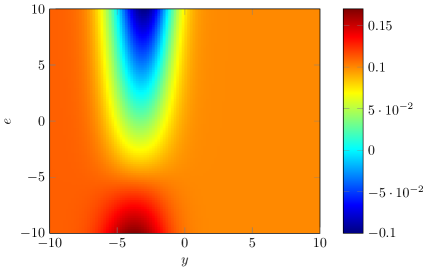
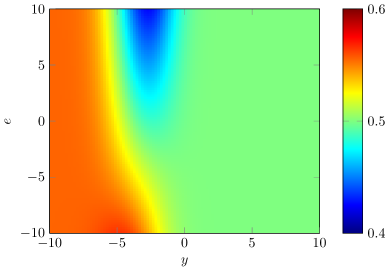
In the next section, we discuss the cases where through numerical implementation of HJB equation (3.13) to determine the region where . An important question in this case is how much the total emission is affected for different choice of parameters and controlled by the regulator.
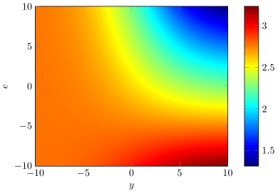
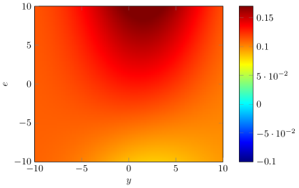
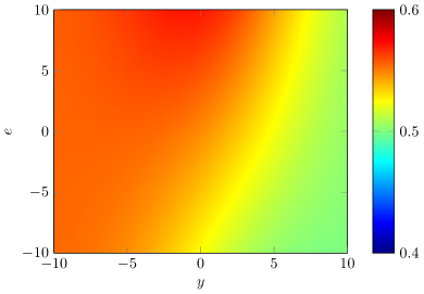
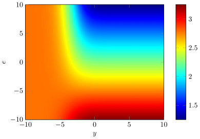
4 Numerical results
The main goal of the numerical results is to understand the behavior of the optimal strategy in (3.16) and more precisely to study the case where . If we consider , , , , and at this moment , then (3.13) reduces to
| (4.1) |
Note that by Lemmas A.12 and A.13, we have and optimal control is given by
where , and we used direct calculations to obtain
To determine the region where , we have to find the region where given by (3.17) is positive, i.e.
For the choice of parameters , () and , we approximated the value function, correction term , and optimal control by a finite-difference Trotter-Kato based scheme whose details is given in Appendix B.
;
;
;
;
;
;
Appendix A Uniqueness, verification and existence of optimal control
Throughout the appendix, we assume that is a filtered probability space satisfying the usual conditions which hosts a Brownian motion and let denote the expectation with respect to . Let
| (A.1) |
where and
| (A.2) |
where are continuous in and Lipschitz in with .
Remark A.1.
Notice that in the current Appendix, the reference probability measure is different from the physical probability measure introduced at the beginning of Section 2. This setting helps us extend the results in this appendix to both value functions and . More precisely, if we set and , then . Else if and , then ; here the dependency of martingale measure with respect to in the definition of is absorbed in the dynamic of .
We would like to show that can be characterized by the HJB equation
| (A.3) |
where
Because of discontinuity in terminal condition, we adopt the definition of discontinuous viscosity solutions from [16, Section 6.2] or [1, Section 4.2] . For a locally bounded measurable function , we denote by and the upper semicontinuous and lower semicontinuous envelopes of , respectively.
Definition A.2.
Let be a locally bounded measurable function. For (A.3) with terminal value ,
-
(a)
a locally bounded measurable function upper semicontinuous on is called a viscosity subsolution if
-
(i)
-
(ii)
for any smooth function such that with , at we have
-
(i)
-
(b)
a locally bounded measurable function lower semicontinuous on is called a viscosity supersolution of (A.3) if
-
(i)
-
(ii)
for any smooth function such that with , at we have
-
(i)
-
(c)
a locally bounded measurable function continuous on is called a viscosity solution of (A.3) if it is both a viscosity sub- and supersolution.
Theorem A.3.
Proof.
By Assumption A, is locally bounded, and can be approximated by a net of continuous functions
Thus, one can apply [16, Theorems 7.4 and 6.8] to obtain (a.ii) and (b.ii) in Definition A.2. To show (a.i) and (b.i), we approximate the terminal condition by two smooth functions and from below and above respectively, i.e. on , on and , and . Then by [16, Theorems 7.4 and 7.6], the value functions and defined below are the unique continuous viscosity solutions333in class of functions with linear growth of problem (A.3) with terminal condition and , respectively.
On the other hand, it follows from the the optimal control problems of , , and that
. Therefore, by taking upper semicontinuous and lower semicontinuous envelopes from both sides and then sending , we obtain the desired result.
For uniqueness, first notice that as . By standard comparison, e.g. [16, Theorem 6.21], Since any upper semicontinuous subsolution (lower semicontinuous supersolution ) of (A.3), is also an upper semicontinuous subsolution (a lower semicontinuous supersolution) of HJB problem for (), we have (). Thus,
and by sending , we obtain uniqueness for .
∎
Remark A.4.
The above continuity result does not imply that . In fact, it only implies that . In this case, the uniqueness may be violated along the half-line . But, we can see that it does not affect the main results of this study.
Theorem A.3 requires minimal regularity of the value function . However to achieve the results of Section 3 for the large production firm, we need to show that an optimal control exists and can be expressed in terms of derivatives of . To do so, we need to impose Assumption Y.
Assumption Y.
are and there is some positive constant , such that for all .
Remark A.5.
The above assumption implies that the semigroup , generated by operator on a bounded regular domain with continuous boundary conditions, is in , in the sense that for any bounded measurable function , for all ; see proof of [9, Theorem 2.10.1].
Lemma A.6.
Let Assumption Y holds. Then, for all .
Proof.
Consider the (not necessarily probability) measure defined by
where . Then, one can write where under satisfies , where is a Brownian motion under . Assumption Y implies that Aronson inequality holds for the density of ; in particular, has no atoms. Thus, and since , . ∎
Lemma A.7.
Proof.
For the moment, let . Then, for any , Itô’s formula implies
| (A.4) |
where is a continuous local martingale. Then, supersolution property of implies that
Let be a sequence for in the definition of local martingale such that . By choosing , taking expectation , and sending , we obtain that
The equality in the above holds from Lemma A.6. If , then by Krylov method of shaking coefficients [10, proof of Theorem 2.2], one can find a supersolution such that . Thus, and the proof of the first part is complete after sending .
The first regularity result is covered by the following two lemmas.
Lemma A.8.
is convex and continuous in uniformly on
Proof.
Convexity in follows from that is supremum of linear functions in . For , we can write
where . Thus, and the inequality is uniform on , which completes the proof. ∎
The following corollary follows from the properties of convex functions and the above Lemma.
Corollary A.9.
Right (left) partial derivatives of , i.e. () exists, is non-decreasing and is right(left)-continuous and bounded in .
Remark A.10.
By Corollary A.9, in Definition A.2 of viscosity supersolution solution, a continuously differentiable test function which touches from below satisfies . Therefore, the supersolution property implies that
provided that is continuous for .
In addition, if is continuous, then the above inequality must hold as equality. To see this, consider a point at which we have a strict inequality in the above. It follows from Lemma A.8 and Corollary A.9 that there exists a point such that the above inequality holds at and exists at . This violates the subsolution property of at .
For the subsolution property, the set of the test functions which touch from above is empty unless , i.e. exists.
Following the above remark, one can study the following terminal value problem which shares the same solution with (A.3).
| (A.5) |
To establish the regularity property in and , we present the following Lemma.
Lemma A.11.
Proof.
First observe that by Assumption (A)-(iv) and [17, Theorem 1.7], the viscosity solution to (A.5) is in on for any fixed . Now for fixed , consider the following boundary value problem on parabolic domain
where and
Since is locally bounded, one can apply Duhamel’s principle on to obtain
By Assumption Y, the right hand side in the above and consquently is in for all and . Notice that is a viscosity solution of and which has a uniques solution . Thus, is in for all and . ∎
Lemma A.12.
Lemma A.13.
Proof.
Suppose that . and let be the optimal control for problem A.1 starting at . Then, by direct calculations one can write
Dividing both sides by and sending yields to . One can obtain the other inequality by the fact that according to Lemma A.12, is right-continuous in and has no atoms. If is the optimal control for problem A.1 starting at , then
Sending yields to . ∎
Appendix B Numerical scheme
In this section, we present details of numerical approximation of the nonlinear problem (4.1) from Section 4. The first step is to discretize in time and in -space. Let be the time step and , for . We set a computational bounded domain for the space domain and discretize the computational domain by an appropriately fine grid with , , and . We set the discrete terminal data . To solve (4.1) numerically, we need to set (1) appropriate artificial boundary conditions (a.k.a. ABC) for the computational domain, (2) treatment of discontinuity of the terminal condition, and (3) stable approximation of the semi-linear terms in (4.1).
To properly set the ABC for computational domain, we return to the optimization problem (3.11). If is sufficiently large so that defined by (3.12) satisfies uniformly on , then we can approximate the value function with the following simple deterministic control problem.
In a similar but simpler fashion, at we have , and thus the approximate ABC becomes . We postpone the derivation of boundary condition on or/and for after we present the algorithm.
In order to handle the discontinuity of terminal condition in the algorithm, we adopt a splitting (Trotter-Kato type) method. At each time step, we handle the calculations in to half-steps. In the first half-step, we solve the heat equation with the same boundary conditions as in the previous step. This regularizes the discontinuous terminal condition. In the second half-step, we solve with ABC boundary condition for the current time step.
To treat the semi-linear term in the second half-step above, we write it as the multiplication of and . Notice that the first term is equal to the optimal control . If we calculated the first term by using the first half-step (solution heat equation), then the second half-step is to solve a linear equation . The above discussion is summarized in the following algorithm.
| (B.1) |
To avoid the hassle of setting ABC on both and , we can approximate from one side by . To set the boundary condition at , notice that first order linear PDE (B.1) can easily be solved by the method of characteristics. However, we can only use method of characteristics as long as we stay in the computational domain. More specifically, method of characteristics can give us the solution at ; i.e.
| (B.2) |
Therefore, we use eqrefeqn:char to set ABC at for (B.1) at step 5 in the algorithm is solved, i.e.
Remark B.1.
Estimation (B.2), which is based on the method of characteristics, can be equivalently derived from approximate dynamic programing principle for the following deterministic optimal control problem which corresponds to (B.1).
| (B.3) |
where and . The dynamic programming principle of problem (B.3) over the interval is
Observe that is an approximation of the optimal control on interval . Thus replacing by yields (B.2).
References
- [1] G. Barles, Solutions de viscosité des équations de Hamilton-Jacobi, Springer Verlag, 1994.
- [2] R. Carmona, F. Delarue, G.-E. Espinosa, and N. Touzi, Singular forward–backward stochastic differential equations and emissions derivatives, The Annals of Applied Probability, 23 (2013), pp. 1086–1128.
- [3] R. Carmona, M. Fehr, and J. Hinz, Optimal stochastic control and carbon price formation, SIAM Journal on Control and Optimization, 48 (2009), pp. 2168–2190.
- [4] , Properly designed emissions trading schemes do work!, Centre for Climate Change Economics and Policy and Grantham Research Institute on Climate Change and the Environment, (2009).
- [5] R. Carmona, M. Fehr, J. Hinz, and A. Porchet, Market design for emission trading schemes, Siam Review, 52 (2010), pp. 403–452.
- [6] U. Çetin and M. Verschuere, Pricing and hedging in carbon emissions markets, International Journal of Theoretical and Applied Finance, 12 (2009), pp. 949–967.
- [7] M. Chesney and L. Taschini, The endogenous price dynamics of emission allowances and an application to CO2 option pricing, Applied Mathematical Finance, 19 (2012), pp. 447–475.
- [8] J. Cvitanić, W. Schachermayer, and H. Wang, Utility maximization in incomplete markets with random endowment, Finance and Stochastics, 5 (2001), pp. 259–272.
- [9] A. Friedman, Partial differential equations. holt, rinehart and winston, Inc., New York, 1 (1969), p. 969.
- [10] N. V. Krylov, The rate of convergence of finite-difference approximations for bellman equations with lipschitz coefficients, Applied Mathematics & Optimization, 52 (2005), pp. 365–399.
- [11] M. Liski and J.-P. Montero, A note on market power in an emission permits market with banking, Environmental and Resource Economics, 31 (2005), pp. 159–173.
- [12] , Market power in an exhaustible resource market: The case of storable pollution permits, Documento de Trabajo, (2008).
- [13] J. J. McCarthy, Climate change 2001: impacts, adaptation, and vulnerability: contribution of Working Group II to the third assessment report of the Intergovernmental Panel on Climate Change, Cambridge University Press, 2001.
- [14] W. S. Misiolek and H. W. Elder, Exclusionary manipulation of markets for pollution rights, Journal of Environmental Economics and Management, 16 (1989), pp. 156–166.
- [15] J. Seifert, M. Uhrig-Homburg, and M. Wagner, Dynamic behavior of CO2 spot prices, Journal of Environmental Economics and Management, 56 (2008), pp. 180–194.
- [16] N. Touzi, Optimal stochastic control, stochastic target problems, and backward SDE, vol. 29, Springer, 2012.
- [17] L. Wang, On the regularity theory of fully nonlinear parabolic equations: Ii, Communications on pure and applied mathematics, 45 (1992), pp. 141–178.