Calculation of SU($2$) string tension in the continuum limit by an effective theory of center vortices

Abstract

The area law fall-off for the Wilson loop average has been confirmed by lattice calculations. Using an effective theory for an ensemble of center vortices, we observe the area law fall-off in the continuum limit for the SU($2$) gauge group in three-dimensional Euclidean space-time. The string tension is obtained in terms of the intrinsic properties of the vortices and the parameter describing their interactions. A good qualitative agreement between our results and the lattice ones is observed. In addition, we show that the repulsive force between the vortices increases with temperature. This behavior is expected due to the reduction of vortex structures at higher temperatures, required for the deconfinement regime.

PACS numbers

74.25.Ha, 74.25.Uv, 12.38.Aw, 12.38.Lg.

I Introduction

Quantum Chromodynamics $\left(\text{QCD}\right)$ describes the strong interaction explaining the underlying structure of hadrons in terms of quarks and gluons QCD1 ; QCD2 ; QCD3 . The dynamics of gluons as the mediate particles of strong interactions are governed by the Yang-Mills theory Yang-Mills .

In the ultraviolet regime, the gauge-coupling constant of QCD becomes small so that the asymptotic freedom behavior is dominant, and the perturbative methods can provide a direct description of QCD vacuum in terms of quarks and gluons. Therefore, non-divergent scattering amplitudes for the high-energy regime or the ultraviolet region can be computed WH .

On the other hand, in the infrared regime, the strong gauge-coupling constant nature of QCD leads to non-perturbative problems which are not easily resolved Nambo-Joan1 ; Nambo-Joan2 ; K. Higashijima ; U-Bar ; E. V. Shuryak ; diakonov . Quarks and gluons as the fundamental degrees of freedom of QCD, have not been observed as isolated particles in the low-energy regime. So far, only hadrons including mesons and baryons, have been observed as color singlet objects in nature. This experimental fact reflects the hypothesis of color confinement mechanism as one of the most controversial unsolved issues in particle physics confinement2004 ; Greensite . During the past few decades, many ideas have been proposed to approach this problem based on non-perturbative methods. cho-restricted ; cho-extented ; Faddeev-Niemi ; t Hooft78 ; Cornwall ; t Hooft80 ; t Hooft81 ; t Hooft82 ; Shabanov ; Faddeev-Niemi2

Lattice QCD and phenomenological models can be introduced as the most popular non-perturbative methods to explain the quark confinement cho-restricted ; cho-extented ; Ripka ; Ichie ; lattice1 ; lattice2 ; lattice3 ; lattice3.1 ; Greensite2003 ; lattice4 ; lattice5 ; lattice6 ; lattice7 ; lattice8 ; deldar ; Deldar1 . The attempt to clarify the mechanism of the confinement phenomenon has led to the fact that the QCD vacuum has some non-trivial structure and this structure is responsible for the confinement of quarks inside the hadrons Ichie ; bruckmann . Topological objects like magnetic monopoles, vortices, instantons, dyons, and calorons are among the candidates that can be used to describe the confinement via some phenomenological models Ichie ; Deldar2 ; Deldar3 ; Deldar4 .

Any theory that investigates the confinement mechanism must predict some features like N-ality dependence and Casimir scaling of string tension, and a linear potential between a pair of static quark-antiquark, which are the important properties of the confining force Greensite . However, there is still no comprehensive mechanism that explains all the properties of the QCD in the infrared regime. Therefore, the study of quark confinement is still of main interest to particle physicists.

From lattice QCD simulations, the potential between a pair of quark-antiquark is kondo : $V^{q\bar{q}}(r)=V^{\text{ele}}(r)+V^{\text{mag}}(r)$. Where $V^{\text{ele}}(r)=-\dfrac{A}{r}$ indicates the Coulombic potential which is inversely proportional to the distance between the quark-antiquark pair $r$ columb , and $V^{\text{mag}}(r)=\sigma r$ shows the linear potential which increases with the distance and is proportional to the string tension Ripka ; Ichie .

The area law fall-off for the Wilson loop average is a well-known gauge-invariant criterion to study quark confinement. It leads to a linear potential between a pair of static quark-antiquark Wilson . To study the linear part of the confinement potential, the quenched approximation is used where the dynamical quarks are removed for the infrared regime Greensite , and the confinement mechanism is described by the dynamics of gluons.

One can introduce some collective modes from gluons that are associated with the topological degrees of freedom of the QCD vacuum, and as a result, it is assumed that the QCD vacuum is filled with the topological defects obtained from these collective modes. Ichie ; kondo

In the absence of matter fields, the center vortex model is a promising scenario for quark confinement. Historically, vortex-like structures were introduced in superconductors in 1959 Gorkov . Even though they were not observed at that time, they were recognized a few years later by Abrikosov Abrikosov . It was proposed in various forms by ’t Hooft t Hooft78 ; t Hooft80 ; t Hooft81 ; t Hooft82 , Nielsen and Olesen NO , Ambjorn and Olesen AO , Mack and Petkova Mack ; MP , and Cornwall Cornwall in the late 1970s with a field theoretical approach. The idea is that the QCD vacuum is filled with closed magnetic vortices which can be condensed in the confined phase. If a Wilson loop is linked to a vortex in an SU($N$) gauge group, the Wilson loop obtains a phase equal to $e^{i2\pi k/N}$ ($k=1$ to $N-1$), corresponding to the type of the vortex. As a result, some disorders are created in the lattice which eventually lead to an area law fall-off and the confinement at the end.

Vortices are defined by the center of the SU($N$) gauge group and there exist $(N-1)$ distinct vortices, which are called non-Abelian Z_N vortices. Lattice calculations show that the Z_N type vortices produce full string tension as the Yang-Mills vacuum does. This is an encouraging motivation to study confinement via center vortices. If the center vortices are removed from the lattice, the string tension also disappears DFGO97 ; DFG97 ; DFG98 ; LTER ; ELRT ; GLR .

The vortex picture relies upon center gauge fixing and center projection DFG97 ; DFG98 . The vortices which appear after performing center projection on the lattice, are called projection vortices (or p-vortices).

For SU($2$) gauge group, the string tension obtained from the projected thin center-vortex ensemble reproduces almost $97.7\%$ of the fundamental string tension calculated from the non gauge fixed situation. For SU($3$), this value is $\sim 62\%$ Langfeld . Another important feature of the center vortex picture is that it naturally explains N-ality dependence of the asymptotic string tension. On the other hand, the modified models of vortices like thick center vortices can explain qualitatively the Casimir scaling dependence for higher representations t Hooft80 ; faber ; Debbio ; Deldar2001 ; Deldar2005 . Therefore, the center vortex models can be a promising scenario for quark confinement.

The most common methods of identifying vortices in the lattice simulation are direct maximal center gauge (DMCG) DFG98 and indirect maximal center gauge (IMCG) DFG97 . Using phenomenological models, vortices have been identified by different methods. There are many articles about this subject; for instance, see Refs. t Hooft78 ; samuel . We have also conducted some studies on identifying vortices in the continuum limit of QCD for the SU($2$) and SU($3$) gauge group asmaee ; karimimanesh .

After reviewing the maximal center gauge fixing to identify vortices in Sec. (II), we review the partition function in Sec. (III) by using a technique that has long been used by polymer physicists. The idea is that a condensate of oriented closed strings can be mapped onto a complex scalar field in a field theoretical approach. Some particle physicists have also used this trick; for instance, see Refs. samuel ; stone ; stone78 ; samuel78 ; oxman . Assuming the intrinsic properties for the center vortex loops such as the stiffness and the tension, as well as defining an interaction between the vortices, one can consider an effective partition function for an ensemble of vortices using the polymer technique. In Sec. (IV), we calculate the Wilson loop average in the continuum limit using an ensemble of closed center vortices in three-dimensional Euclidean space-time. We show that the Wilson loop average displays an area law fall-off and the string tension is derived for the SU($2$) gauge group in terms of the intrinsic properties of the center vortices and the parameter which describes the interaction between the vortices. A good qualitative agreement between the plot of the stiffness versus the tension of this calculation and the lattice results is obtained. The repulsive potential between vortices is studied and it is discussed that the strength of the potential shows an appropriate behavior concerning the temperature.

II Introducing vortices in the continuum limit

It has been more than three decades since the properties of the center vortices and their role in quark confinement have been confirmed by lattice QCD; for a good review see reference Greensite2003 .

Direct maximal center gauge $\left(\text{DMCG}\right)$ and indirect maximal center gauge $\left(\text{IMCG}\right)$ are among the most common methods of identifying vortices in lattice simulations. DMCG and IMCG are introduced to perform maximal center gauge fixing and center projection to identify vortices. Other methods for identifying vortices were also proposed in lattice QCD. Examples are Laplacian center gauge fixing by de Forcrand et al. LCGF ; LCGF1 and direct Laplacian center gauge fixing by Langfeld et al. Langfeld2001 and Faber et al. Faber . All of these methods yield qualitatively similar results.

Center vortices are defined by the centers of the SU($N$) gauge group and carry magnetic fluxes corresponding to the centers, Z($N$). The magnetic fluxes are associated with the non-trivial center elements $z_{k}=\text{exp}\left(i\dfrac{2\pi}{N}k\right)\textbf{1}_{N\times N},\left(k=1,2,...,N-1\right)$ of Z($N$) discrete gauge group. For SU($2$) gauge group, the non-trivial center element corresponds to -1 and the trivial center element to +1, where 1 represents a $2\times 2$ unit matrix. The center vortices are defined as a string, surface and volume in $D=2$, $3$ and $4$, respectively.

It is assumed that the center vortices carrying magnetic fluxes, squeeze the electric fields between a quark-antiquark pair inside a flux tube. If a Wilson loop is linked to a vortex in an SU($N$) gauge group, it obtains a phase equal to the center element, corresponding to the type of the vortex. As a result, some disorders are created in the lattice which eventually lead to an area law fall-off.

In this section, we review the emergence of vortices in the continuum limit which we have reported in reference asmaee . Inspired by DMCG method in lattice QCD which confirms the existence of vortices using the maximal center gauge fixing and center projection, we have shown that vortices are identified by performing a singular gauge transformation. Linking the Wilson loop and the vortices, the Wilson loop gets a phase equal to the non-trivial center elements associated with $z$($k$),

$$W(C)\longrightarrow z(k)W(C).$$ (1)

The non-trivial center elements $z(k)$ of SU($N$) group are given as,

$$z(k)=e^{i\frac{2\pi}{N}k}\textbf{1},\quad\left(k=1,2,...,N-1\right),$$ (2)

where 1 represents an $N\times N$ unit matrix. On the other hand, the center elements $z(k)$ can be rewritten as the following oxman

$$z(k)=e^{i2\pi\nu(k)},\quad\nu(k)=\nu^{a}(k)H_{a},$$ (3)

where $\nu(k)$ are co-weights and $H_{a}$’s indicate the generators of the Cartan subalgebra.

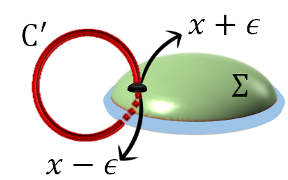
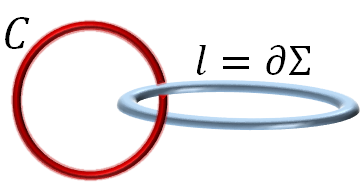
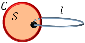
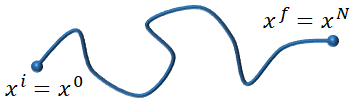
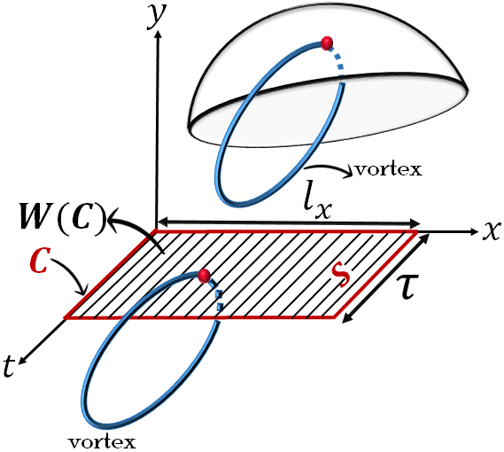
In three-dimensional space-time, a non-trivial contribution to the Wilson loop operator is obtained by the linking number $L\left(C,l\right)$ between the Wilson loop $C$ and the vortex loop $l$. Where $l$ indicates the boundary of the hypersurface $\Sigma$ $\left(\text{ i.e.}\ l=\partial\Sigma\right)$ shown in Fig. 1(b). The linking number can also be described in other alternative ways: by the intersection number $I\left(C,\Sigma\right)$ between the Wilson loop $C$ and the hypersurface $\Sigma$ shown in Fig. 1(a), or by the intersection number $I\left(S,l\right)$ between the Wilson surface $S$ and the vortex loop $l$ (see Fig. 1(c)). These three definitions are equivalent: $L\left(C,l\right)=I\left(C,\Sigma\right)=I\left(S,l\right)$ kondo . We recall that the linking number and the intersection number are integers.

(a)

(b)

(c)

Figure 1: (a) Intersection between the Wilson loop $C$ and hypersurface $\Sigma$. (b) Linking between the Wilson loop $C$ and a vortex loop $l$ which is the boundary of hypersurface, $l=\partial\Sigma$. (c) Intersection between the Wilson surface $S$ and the vortex loop $l$.

Under a center gauge transformation $N(x)\in$ SU($2$), the contribution of the thin vortex defined on the closed loop $l=\partial\Sigma$ for $x\neq\Sigma$ is asmaee ; ER2017 ,

$$\text{thin\ vortex}=\dfrac{i}{g}N(x)\partial_{\mu}N^{\dagger}(x),\quad x\notin\Sigma.$$ (4)

For SU($2$) group, the appropriate center gauge transformation is asmaee ,

$$N=e^{i\varphi T^{3}}=\left(\begin{matrix}e^{i\frac{\varphi}{2}}&0\\ 0&e^{-i\frac{\varphi}{2}}\end{matrix}\right),\quad\varphi\in\left[0,2\pi\right),$$ (5)

where $\varphi$ is the azimuth angle in cylindrical coordinates and $T^{3}$ is equal to the half of the Pauli matrix $\sigma^{3}$. Replacing Eq. (5) in Eq. (4), the contribution of the thin vortex is,

$$\text{thin\ vortex}\equiv A_{\mu}^{l}(x)=\vec{A}_{\mu}^{l}.\vec{T}=\dfrac{i}{g}N\partial_{\mu}N^{\dagger}=\dfrac{1}{g}\partial_{\mu}\varphi T^{3}.$$ (6)

The spatial component of the thin vortex is,

$$\vec{A}_{\varphi}^{l}.\vec{T}=\dfrac{1}{g\rho}T^{3},\quad\vec{A}_{\rho}^{l}.\vec{T}=0.$$ (7)

Equation (7) represents the gauge field associated with the thin vortex in cylindrical coordinates. The thin vortex is observed at $\rho=0$ in the third direction of color space. The magnetic vortex flux $\Phi^{\text{flux}}$ is,

$$\begin{split}\Phi^{\text{flux}}&=\int dx_{\mu}\left(\vec{A}_{\mu}^{l}.\vec{T}\right)=\dfrac{1}{2g}\int^{2\pi}_{0}d\varphi\left(\begin{matrix}1&0\\ 0&-1\end{matrix}\right)\\ &=\dfrac{2\pi}{g}T^{3}.\end{split}$$ (8)

We would like to calculate the Wilson loop average from the vortex ensemble. The center gauge fixing imposed on the SU($2$) Yang-Mills theory is assumed to be similar to the center gauge fixing on a lattice. Therefore, the contribution of the vortex field $A_{\mu}^{l}$ to the Wilson loop is as the following,

$$W_{\text{vortex}}(C)\equiv e^{i\oint_{C}dx_{\mu}A_{\mu}^{l}(x)}.$$ (9)

On the other hand, when the thin vortex loop $l$ intersects the Wilson surface $S$, the Wilson loop obtains a factor as the following,

$$W_{\text{vortex}}(C)=z^{I(S,l)},$$ (10)

where $z$ is the non-trivial center element of the SU($2$) gauge group. Replacing Eq. (3) for SU($2$) group in Eq. (10),

$$W_{\text{vortex}}(C)=e^{i2\pi\nu I(S,l)}.$$ (11)

Using Eqs. (9) and (11), the relationship between intersection number and the line integral of a vortex field $A_{\mu}^{l}$ is as follows,

$$\oint_{C}dx_{\mu}A_{\mu}^{l}(x)=2\pi\nu I(S,l).$$ (12)

An explicit integral formula for the intersection $I\left(S,l\right)$ between the Wilson surface $S$ and the vortex loop $l$ is defined kondo ,

$$\begin{split}&I\left(S,l\right)=\dfrac{1}{4\pi}\oint_{l=\partial\Sigma}dx_{\mu}\int_{S}d^{2}{\sigma}_{\mu}\delta^{\left(3\right)}\left(x-\bar{x}\left(\sigma\right)\right),\\ &d^{2}{\sigma}_{\mu}=\epsilon_{\mu\nu\rho}\dfrac{\partial\bar{x}_{\nu}}{\partial\sigma_{1}}\dfrac{\partial\bar{x}_{\rho}}{\partial\sigma_{2}}d\sigma_{1}d\sigma_{2},\end{split}$$ (13)

where $d^{2}{\sigma}_{\mu}$ is the surface element and $S$ is parameterized by $\bar{x}\left(\sigma\right)=\bar{x}\left(\sigma_{1},\sigma_{2}\right)$.

Replacing Eq. (13) in Eq. (12),

$$\oint_{C}dx_{\mu}A_{\mu}^{l}(x)=\dfrac{\nu}{2}\oint_{l=\partial\Sigma}dx_{\mu}\int_{S}d^{2}{\sigma}_{\mu}\delta^{\left(3\right)}\left(x-\bar{x}\left(\sigma\right)\right).$$ (14)

The vector field $J_{\mu}^{C}$ is defined on the Wilson surface $S$ as the following,

$$J_{\mu}^{C}(x)\equiv\dfrac{\nu}{2}\int_{S}d^{2}\sigma_{\mu}\delta^{\left(3\right)}\left(x-\bar{x}\left(\sigma\right)\right).$$ (15)

Replacing Eq. (15) in Eq. (14),

$$\oint_{C}dx_{\mu}A_{\mu}^{l}(x)=\oint_{l}dx_{\mu}J_{\mu}^{C}(x).$$ (16)

The linking number $L(C,l)$ is symmetric with respect to the interchange of the loops $C$ and $l$: $L(C,l)=L(l,C)$. Applying this interchange to the previous equation, one obtains a noticeable result. The vortex field $A_{\mu}^{l}$ and the vector field $J_{\mu}^{l}$ are somehow equivalent. The vortex field $A_{\mu}^{l}$ which is defined on the closed loop $l$ can be gauge transformed to the vector field $J_{\mu}^{l}$. Indeed, when $n$ vortices intersect the Wilson surface, the flux of all $n$ vortices passes through the surface $S$ $\left(\text{see\ Fig.}\ \ref{fig2}\right)$, therefore, the vector field $J_{\mu}^{C}$ in Eq. (15) indicates the gauge potential of the vortex field which its worldline $l$ is replaced by $C$ oxman .

Figure 2: $n$ vortices intersecting the Wilson surface $S$ bounded by the closed loop $C$.

It is useful to rewrite Eq. (16) as the following,

$$\begin{split}\oint_{C}dx_{\mu}A_{\mu}^{l}(x)=\oint_{l}dx_{\mu}J_{\mu}^{C}(x)&=\int_{0}^{L}ds\dfrac{dx_{\mu}}{ds}J_{\mu}^{C}(x(s))\\ &=\int_{0}^{L}dsu_{\mu}(s)J_{\mu}^{C}\left(x\left(s\right)\right),\end{split}$$ (17)

where $L$ is the total length of the vortex worldline and $s$ is the arc length parameter of the vortex loop which runs from $0$ to $L$, and $u_{\mu}(s)$ is a tangent vector to the $s$.

Replacing (17) in Eq. (9), the Wilson loop average is,

$$W_{\text{vortex}}(C)=e^{i\int_{0}^{L}dsu_{\mu}(s)J_{\mu}^{C}\left(x(s)\right)}.$$ (18)

From the above equation and Fig. 2, if $n$ vortices intersect the Wilson surface $S$,

$$W_{\text{vortex}}(C)=e^{i\sum_{i=1}^{n}\int_{0}^{L_{i}}ds_{i}u_{\mu}(s_{i})J_{\mu}^{C}(x(s_{i}))}.$$ (19)

In fact, $J_{\mu}^{C}(x)$ describes a general vector field containing the flux of the $n$ vortices passing through surface $S$.

III Partition function for an ensemble of center vortices

To calculate the linear potential between a pair of quark-antiquark and the string tension in three-dimensional Euclidean space-time, we use the partition function of an ensemble of center vortices. To obtain an effective partition function, one can use a trick that for a long time has been used by polymer physicists, and particle physicists have used that, as well. The idea is that a condensate of oriented closed strings can be mapped onto a complex scalar field. The action is written in terms of the interacting vortices and intrinsic properties of the vortex loops such as the tension and stiffness.

The action of an ensemble of $n$ vortices can be written as the following oxman ; stiff1 ; stiff2 ; stiff3 ,

$$S^{0}_{n}=\sum_{i=1}^{n}\int_{0}^{L_{i}}ds_{i}\left[\mu+\dfrac{1}{2\kappa}\left(\dfrac{du_{\mu}(s_{i})}{ds_{i}}\right)^{2}\right],$$ (20)

where $\mu$ indicates the action per length and is called the tension of the center vortex. The parameter $\dfrac{1}{\kappa}$ shows the stiffness of the vortices and it is small for flexible vortices. The structure of a vortex is described by a space curve $x(s)$ in which $s\in\left[0,L\right]$ is a parameter denoting the arc length along the vortex backbone. The vector $u\left(s\right)=\frac{dx\left(s\right)}{ds}$ is a tangent vector and $\frac{du\left(s\right)}{ds}=\frac{d^{2}x\left(s\right)}{ds^{2}}$ is interpreted as the local curvature of the vortex. Fredrickson

To make the model more physical, one should assume a potential that represents the interaction between the vortices. Therefore, a delta-function type potential $V(x_{i}-x_{j})$ is assumed oxman ,

$$V(x_{i}-x_{j})=\dfrac{1}{\zeta}\delta^{\left(3\right)}(x_{i}-x_{j}),\quad\zeta>0.$$ (21)

We call the parameter $\dfrac{1}{\zeta}$ as the strength of the potential. The action corresponding to Eq. (21), shown the vortices interaction is,

$$\begin{split}S^{\text{int}}_{n}&=\dfrac{1}{2}\sum_{i,j=1}^{n}\int_{0}^{L_{i}}\int_{0}^{L_{j}}ds_{i}ds_{j}V(x_{i}(s_{i}),x_{j}(s_{j}))\\ &=\dfrac{1}{2\zeta}\sum_{i,j=1}^{n}\int_{0}^{L_{i}}\int_{0}^{L_{j}}ds_{i}ds_{j}\delta^{\left(3\right)}(x_{i}(s_{i})-x_{j}(s_{j})).\end{split}$$ (22)

Using Eqs. (20) and (22), the action of the vortex ensemble is obtained as the sum of the non-interacting part $S^{0}_{n}$ and the interacting part $S^{\text{int}}_{n}$,

$$S^{\text{total}}_{n}=S^{0}_{n}+S^{\text{int}}_{n}.$$ (23)

Next, an interaction between the Wilson loop, defined by the vector field $J_{\mu}^{C}(x)$ in Eq. (19), and the vortex ensemble is assumed. Using Eqs. (19) and (23), the partition function of the ensemble of $n$ vortices and the Wilson loop is written as,

$$Z\left[J_{\mu}^{C}\right]=\sum_{n}\int\left[Dl\right]_{n}e^{i\sum_{i=1}^{n}\int_{0}^{L_{i}}ds_{i}u_{\mu}(s_{i})J^{C}_{\mu}(x(s_{i}))}e^{-S^{\text{total}}_{n}},$$ (24)

where,

$$\left[Dl\right]_{n}\equiv\dfrac{1}{n!}\prod_{i=1}^{n}\int_{0}^{\infty}\dfrac{dL_{i}}{L_{i}}\prod_{j=1}^{n}\int dv_{j}\prod_{k=1}^{n}\int\left[Dv\left(s_{k}\right)\right]_{v_{k},v_{k}}^{L_{k}},$$ (25)

The measure $\left[Dl\right]_{n}$ integrates over all possible states of the $n$ vortices. The measure $dL_{i}$ integrates on vortex worldlines which have a fixed length of $L$. The measures $dv_{j}=d^{3}x_{j}d^{2}u_{j}$ and $\left[Dv\left(s_{k}\right)\right]_{v_{k},v_{k}}^{L_{k}}$ correspond to the vortex loop oxman .

For no intersection between the Wilson surface and the vortices, the vector field $J^{C}_{\mu}$ is zero and the partition function of the vortex ensemble is $Z\left[J^{C}_{\mu}=0\right]\equiv Z\left[0\right]=\sum_{n}\int\left[Dl\right]_{n}e^{-S^{\text{total}}_{n}}$. Therefore, one can define the Wilson loop average in terms of the two partition functions,

$$\left\langle W(C)\right\rangle=\dfrac{Z[J^{C}_{\mu}]}{Z[0]}.$$ (26)

In Sec. IV, using Eq. (26) we obtain the area law fall-off for the Wilson loop average.

To get a more efficient statement for the partition function, $e^{-S^{\text{int}}_{n}}$ in Eq. (22) can be rewritten in terms of a scalar vortex density $\rho(x)$, defined as the following,

$$\rho(x)\equiv\sum_{i=1}^{n}\int_{0}^{L_{i}}ds_{i}\delta^{(3)}(x-x_{i}(s_{i})).$$ (27)

Using Eq. (27),

$$e^{-\frac{1}{2\zeta}\int d^{3}x\rho^{2}}=e^{-S^{\text{int}}_{n}}.$$ (28)

${W[\phi]}$ is defined in terms of the scalar field $\phi$,

$$W[\phi]\equiv\int d^{3}x\phi^{2}(x).$$ (29)

Using Eq. (29) and the Gaussian formula, Eq. (28) is obtained from the left hand side of the following expression,

$$\dfrac{1}{\sqrt{\pi}}\int\left[D\phi\right]e^{-W[\phi]}e^{i\sqrt{\frac{2}{\zeta}}\int d^{3}x\rho(x)\phi(x)}=e^{-S^{\text{int}}_{n}}.$$ (30)

Replacing Eqs. (20), (23) and (30) in Eq. (24),

$$Z\left[J^{C}_{\mu}\right]=\dfrac{1}{\sqrt{\pi}}\int\left[D\phi\right]e^{-W[\phi]}\sum_{n}\int\left[Dl\right]_{n}e^{-\sum_{i=1}^{n}\int_{0}^{L_{i}}ds_{i}\left[w(x_{i},u_{\mu}(s_{i}))+\frac{1}{2\kappa}\dot{u}_{\mu}^{2}(s_{i})\right]},$$ (31)

where

$$w(x_{i},u_{\mu}(s_{i}))\equiv\mu-i\left(u_{\mu}(s_{i})J^{C}_{\mu}(x(s_{i}))+\sqrt{\dfrac{2}{\zeta}}\phi(x_{i})\right).$$ (32)

In order to calculate the partition function of Eq. (31), particle physicists use the trick introduced by polymer physicists which we are going to briefly explain.

(a)

(b)

(c)

(d)

Figure 3: (a) A continuous curve between $x^{i}$ and $x^{f}$, (b) the polymer approximation of (a). (c) a closed curve, (d) the polymer approximation of (c).

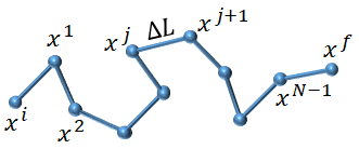
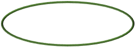
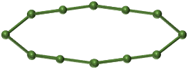
The continuous curve of Fig. 3(a), is divided into $N$ parts shown in Fig. 3(b). It resembles a polymer with the vertices acting as atoms (or monomers) and the segments acting as bonds. The polymer of Fig. 3(b) extends from $x^{i}$ to $x^{f}$ via $x^{1},x^{2},...,x^{\left(N-1\right)}$ and each bond has a fixed length equal to $\epsilon$. Therefore, the total length of the polymer is equal to $N\epsilon.$ Similarly, a vortex of worldline of length $L$ can be divided into $N$ parts with fixed length $\epsilon$ and the extension of the vortex is assumed to be from $x^{0}$ to $x^{N}$. To get the continuum, $\epsilon\rightarrow 0$ and $N\rightarrow\infty$, and finally the vortex loop is obtained if $x^{i}=x$, $x^{f}=x$ (see Fig. 3(c)). The polymer approximation of a loop shown in Fig. 3(c) is brought in Fig. 3(d)).

Replacing the measure $[Dl]_{n}$ of Eq. (25) in Eq. (31), the partition function for the vortex worldline with length $L$ which extends from $x^{0}$ identified by $u_{\mu}^{0}$ to $x^{N}$ identified by $u_{\mu}^{N}$ is,

$$Z\left[J^{C}_{\mu}\right]=\dfrac{1}{\sqrt{\pi}}\int\left[D\phi\right]\ e^{-W[\phi]}\ \text{exp}\left\{\int_{0}^{\infty}\dfrac{dL}{L}\int dvq\left(v,v,L\right)\right\}$$ (33)

$q\left(v^{N},v^{0},L\right)$ is defined as the following,

$$q\left(v^{N},v^{0},L\right)=\int\left[Dv\left(s_{k}\right)\right]_{v^{N},v^{0}}^{L}e^{-\int_{0}^{L}ds\left[w(x,u_{\mu}(s))+\frac{1}{2\kappa}\left(\dot{u}_{\mu}(s)\right)^{2}\right]}.$$ (34)

It is called the end-to-end distance probability distribution for the vortex worldline with length $L$, which goes from $x^{0}$ to $x^{N}$ (see Fig. 3(a)). Therefore, $\int dvq\left(v,v,L\right)$ in the last equality of Eq. (33) represent the partition function of a vortex loop with fixed length $L$. Setting $v^{N}=v^{0}=v$ in Eq. (34), we obtain $q$ for a loop needed in Eq. (33).

$$q\left(x^{N},u^{N};x^{0},u^{0};L\right)=\int\prod_{i=1}^{N-1}d^{3}x^{i}d^{2}u^{i}\prod_{j=1}^{N}e^{-\epsilon w\left(x^{j}(s^{j}),u^{j}\right)}\prod_{k=1}^{N}\psi\left(u^{k}-u^{k-1}\right)\delta^{(3)}\left(x^{k}-x^{k-1}-u^{k}\epsilon\right),$$ (35)

where $\psi\left(u^{k}-u^{k-1}\right)\equiv e^{-\frac{1}{2\kappa}\epsilon\left(\frac{u^{k}-u^{k-1}}{\epsilon}\right)^{2}}$.

On the other hand, the relation between $q\left(v^{N},v^{0},L\right)$ and $q\left(x^{N},u^{N};x^{0},u^{0};L\right)$ is defined as,

$$q\left(v^{N},v^{0},L\right)=\lim_{N\rightarrow\infty}q\left(x^{N},u^{N};x^{0},u^{0};L\right).$$ (36)

Separating one of the segments, for example, the last one, from the others and keeping the rest as a string with the length $L-\epsilon$, we can rewrite (35) as the following,

$$q\left(x^{N},u^{N};x^{0},u^{0};L\right)=e^{-\epsilon w\left(x^{N}(s^{N}),u^{N}\right)}\int d^{2}u^{N-1}\psi\left(u^{N}-u^{N-1}\right)q\left(x^{N}-u^{N}\epsilon,u^{N-1};x^{0},u^{0};L-\epsilon\right).$$ (37)

where $q\left(x^{N-1},u^{N-1};x^{0},u^{0},L-\epsilon\right)$ is the end-to-end distance probability distribution for the vortex worldline with length $L-\epsilon$ extending from $x^{0}$ to $x^{N-1}$.

Taylor expanding both sides of Eq. (37), and keeping the terms to the first order in $\epsilon$, one finds that,

$$\partial_{L}q\left(x^{N},u^{N};x^{0},u^{0};L\right)=\left[\dfrac{\kappa}{2}\nabla^{2}_{u}-\mu+i\sqrt{\frac{2}{\zeta}}\phi(x_{N})-u^{N}.D_{\mu}\right]q\left(x^{N},u^{N};x^{0},u^{0};L\right),\quad D_{\mu}=\nabla_{x^{N}}-iJ^{C}_{\mu}(x^{N}),$$ (38)

where $D_{\mu}$ is the covariant derivative and $\nabla_{u}^{2}$ is the Laplacian operator on the unit sphere.

Equation (38) can be solved with the following initial conditions,

$$q\left(x^{N},u^{N};x^{0},u^{0};L=0\right)=\delta^{\left(3\right)}\left(x^{N}-x^{0}\right)\delta^{\left(2\right)}\left(u^{N}-u^{0}\right).$$ (39)

For the small stiffness limit, corresponding to large $\kappa$, we can use the methods of Refs. oxman ; Fredrickson ; oxman1 and finally, the solution can be approximated by,

$$q\left(x^{N},u^{N};x^{0},u^{0};L\right)\approx\dfrac{1}{4\pi}\left\langle x^{N}\left|e^{-L\hat{O}}\right|x^{0}\right\rangle,$$ (40)

where

$$\hat{O}=-\dfrac{1}{3\kappa}D_{\mu}D_{\mu}+\mu-i\sqrt{\dfrac{2}{\zeta}}\phi.$$ (41)

Replacing Eq. (40) in the exponential of Eq. (33) for $x^{N}=x^{0}=x$,

$$\begin{split}\int_{0}^{\infty}\dfrac{dL}{L}\int dvq\left(v,v;L\right)&=\int_{0}^{\infty}\dfrac{dL}{L}\int d^{3}x\left\langle x\left|e^{-L\hat{O}}\right|x\right\rangle\\ &=\int_{0}^{\infty}\dfrac{dL}{L}\ \text{Tr}\ e^{-L\hat{O}}=\text{Tr}\ln\hat{O}.\end{split}$$ (42)

And we use the following equation,

$$\exp\left\{-\text{Tr}\ln\hat{O}\right\}=\int D\bar{V}DV\ e^{-\int d^{3}x\bar{V}\hat{O}V}.$$ (43)

Replacing Eqs. (29),(41), (42) and (43) into Eq. (33), the partition function $Z[J^{C}_{\mu}]$ is,

$$\begin{split}Z\left[J^{C}_{\mu}\right]&=\dfrac{1}{\sqrt{\pi}}\int\left[D\phi\right]\ e^{-W[\phi]}\int D\bar{V}DV\ e^{-\int d^{3}x\bar{V}\left(-\frac{1}{3\kappa}D_{\mu}D_{\mu}+\mu-i\sqrt{\frac{2}{\zeta}}\phi\right)V}\\ &=\dfrac{1}{\sqrt{\pi}}\int D\bar{V}DV\ e^{-\int d^{3}x\left(\frac{1}{3\kappa}\bar{D}_{\mu}\bar{V}D_{\mu}V+\mu\bar{V}V\right)}\int\left[D\phi\right]\ e^{\int d^{3}x\left(-\phi^{2}+i\sqrt{\frac{2}{\zeta}}\bar{V}V\phi\right)}\\ &=\int D\bar{V}DV\ e^{-\int d^{3}x\left(\frac{1}{3\kappa}\bar{D}_{\mu}\bar{V}D_{\mu}V+\mu\bar{V}V+\frac{1}{2\zeta}\left(\bar{V}V\right)^{2}\right)},\end{split}$$ (44)

in the last equality, the Gaussian formula is used to calculate the second integral and $V$ is a complex field.

In this section, we have explained how one can obtain an effective partition function for a vortex ensemble using the trick of polymer physicists. In the next section, we use the effective partition function Eq. (44) to compute the Wilson loop average and we obtain the area law fall-off which leads to the linear potential between a pair of static quark-antiquark and at the end the string tension is extracted. The dependence of the string tension on the vortex parameters and the temperature are discussed in detail.

IV the Wilson loop average in the presence of the center vortices - the area law fall-off

From the partition function of Eq. (44), the Lagrangian of the vortex ensemble is understood to be,

$$\mathcal{L}=\dfrac{1}{3\kappa}\bar{D}_{\mu}\bar{V}D_{\mu}V+\underbrace{\mu\bar{V}V+\dfrac{1}{2\zeta}\left(\bar{V}V\right)^{2}}_{\equiv\mathbf{V}\left(\bar{V},V\right)},$$ (45)

The Lagrangian $\mathcal{L}$ is invariant under a global U($1$) gauge transformation. The vacuum expectation value $v$ is obtained by minimizing the potential $\mathbf{V}\left(\bar{V},V\right)$,

$$v^{2}=-\mu\zeta>0,\quad\mu<0.$$ (46)

The complex scalar field $V(x)$ can be defined as,

$$V(x)=ve^{i\gamma(x)}.$$ (47)

The scalar field $\gamma(x)$ is a modulo $2\pi$ function so that a set of degenerate vacua are related to each other. Rewriting the potential $\mathbf{V}\left(\bar{V},V\right)$ in terms of the vacuum expectation value $v$, the partition function is,

$$Z\left[J^{C}_{\mu}\right]=\int D\bar{V}DV\ e^{-\int d^{3}x\left(\frac{1}{3\kappa}\bar{D}_{\mu}\bar{V}D_{\mu}V+\frac{1}{2\zeta}\left(\bar{V}V-v^{2}\right)^{2}\right)}.$$ (48)

To compute the Wilson loop average in the presence of the vortices, we use Eqs. (26) and (48).

We recall that when there is no intersection between the Wilson surface and the vortices, the vector field $J^{C}_{\mu}$ is zero and the covariant derivative $D_{\mu}=\partial_{\mu}-igJ^{C}_{\mu}$ is replaced by the partial derivative $\partial_{\mu}$. Therefore, using Eq. (48), the partition function $Z[0]$ is,

$$Z[0]=\int D\bar{V}DVe^{-\int d^{3}x\left(\frac{1}{3\kappa}\partial_{\mu}\bar{V}\partial_{\mu}V+\frac{1}{2\zeta}\left(\bar{V}V-v^{2}\right)^{2}\right)}.$$ (49)

Then, the Wilson loop average is calculated as the following,

$$\left\langle W(C)\right\rangle=\dfrac{Z[J^{C}_{\mu}]}{Z[0]}=\dfrac{\int D\bar{V}DV\ e^{-\int d^{3}x\left(\frac{1}{3\kappa}\bar{D}_{\mu}\bar{V}D_{\mu}V+\frac{1}{2\zeta}\left(\bar{V}V-v^{2}\right)^{2}\right)}}{\int D\bar{V}DVe^{-\int d^{3}x\left(\frac{1}{3\kappa}\partial_{\mu}\bar{V}\partial_{\mu}V+\frac{1}{2\zeta}\left(\bar{V}V-v^{2}\right)^{2}\right)}}=\dfrac{\int D\bar{V}DV\ e^{-\int d^{3}x\frac{1}{3\kappa}\bar{D}_{\mu}\bar{V}D_{\mu}V}}{\int D\bar{V}DVe^{-\int d^{3}x\frac{1}{3\kappa}\partial_{\mu}\bar{V}\partial_{\mu}V}}.$$ (50)

The last equality is obtained by expansion of the complex scalar field V around the vacuum expectation value.

The partition function $Z[0]$ in Eq. (50) is defined in the absence of any linking between the vortices and the Wilson loop,

$$Z[0]=\int D\bar{V}DVe^{-\int d^{3}x\frac{1}{3\kappa}\partial_{\mu}\bar{V}\partial_{\mu}V}.$$ (51)

Using Eq. (47),

$$\partial_{\mu}\bar{V}(x)\partial_{\mu}V(x)=v^{2}\left(\partial_{\mu}\gamma(x)\right)^{2}.$$ (52)

Replacing Eq. (52) in Eq. (51), the partition function $Z[0]$ is,

$$Z[0]=N^{\prime}v^{2}\int D\gamma e^{-\frac{v^{2}}{3\kappa}\int d^{3}x\left(\partial_{\mu}\gamma(x)\right)^{2}},$$ (53)

where $N^{\prime}$ is an overall normalization factor and is irrelevant. Equation (53) expresses the partition function $Z[0]$ as a functional integral on $\gamma$. In three-dimensional Euclidean space-time kapusta ,

$$\begin{split}S_{0}&\equiv-\frac{v^{2}}{3\kappa}\int d^{3}x\left(\partial_{\mu}\gamma(x)\right)^{2}\\ &=-\frac{v^{2}}{3\kappa}\int^{\beta}_{0}dt\int d^{2}x\left[\left(\frac{\partial\gamma(x)}{\partial t}\right)^{2}+\left(\nabla\gamma(x)\right)^{2}\right]\\ &=-\frac{v^{2}}{3\kappa}\int^{\beta}_{0}dt\int d^{2}x\gamma(x)\left(-\frac{\partial^{2}}{\partial t^{2}}-\nabla^{2}\right)\gamma(x).\end{split}$$ (54)

Next, we use a Fourier expansion for the scalar field $\gamma(x)$ kapusta ,

$$\gamma(x)=\gamma\left(t,x,y\right)=\gamma\left(t,\vec{x}\right)=\sum_{n=-\infty}^{\infty}\sum_{\vec{p}}e^{i\left(w_{n}t+\vec{p}.\vec{x}\right)}\gamma_{n}(\vec{p}),$$ (55)

where $w_{n}=2\pi nT$ and $T$ is the temperature. Using Eq. (55),

$$\begin{split}&\frac{\partial^{2}\gamma(x)}{\partial t^{2}}=-\sum_{n=-\infty}^{\infty}\sum_{\vec{p}}w_{n}^{2}e^{i\left(w_{n}t+\vec{p}.\vec{x}\right)}\gamma_{n}(\vec{p}).\\ &\nabla^{2}\gamma(x)=\frac{\partial^{2}\gamma(x)}{\partial x^{2}}+\frac{\partial^{2}\gamma(x)}{\partial y^{2}}\\ &\quad\quad\quad\ =-\sum_{n=-\infty}^{\infty}\sum_{\vec{p}}\vec{p}^{2}e^{i\left(w_{n}t+\vec{p}.\vec{x}\right)}\gamma_{n}(\vec{p}),\quad\vec{p}^{2}=\vec{p}^{2}_{x}+\vec{p}^{2}_{y}.\end{split}$$ (56)

Replacing Eq. (56) in Eq. (54),

$$S_{0}=-\dfrac{v^{2}\mathtt{V}}{3\kappa}\sum_{n=-\infty}^{\infty}\sum_{\vec{p}}\left(w_{n}^{2}+\vec{p}^{2}\right)\left|\gamma_{n}(\vec{p})\right|^{2},$$ (57)

where $\mathtt{V}\equiv\beta L^{2}$ is the volume and $L$ indicates the spatial length and $\beta$ represents the imaginary time. Using Eq. (57) in Eq. (53) for the action, the partition function $Z[0]$ is,

$$\begin{split}Z[0]&=N^{\prime}v^{2}\prod_{n=-\infty}^{\infty}\prod_{\vec{p}}\ \int d\gamma_{n}(\vec{p})\ e^{-\frac{v^{2}\mathtt{V}}{3\kappa}\left(w_{n}^{2}+\vec{p}^{2}\right)\left|\gamma_{n}(\vec{p})\right|^{2}}\\ &=N^{\prime}v^{2}\prod_{n=-\infty}^{\infty}\prod_{\vec{p}}\left(\dfrac{3\kappa\pi}{v^{2}\mathtt{V}}\right)^{\frac{1}{2}}\left[w_{n}^{2}+\vec{p}^{2}\right]^{-\frac{1}{2}}.\end{split}$$ (58)

In the second equality, the Gaussian integral formula is used.

Next, we calculate the partition function $Z[J^{C}_{\mu}]$ in Eq. (50). We recall that it shows the case where the Wilson loop links the vortices,

$$Z[J^{C}_{\mu}]=\int D\bar{V}DV\ e^{-\frac{1}{3\kappa}\int d^{3}x\bar{D}_{\mu}\bar{V}D_{\mu}V}.$$ (59)

Replacing the definition of the covariant derivative $D_{\mu}=\partial_{\mu}-iJ^{C}_{\mu}$ in the above equation,

$$Z[J^{C}_{\mu}]=\int D\bar{V}DV\ e^{-\frac{1}{3\kappa}\int d^{3}x\partial_{\mu}\bar{V}(x)\partial_{\mu}V(x)}\ e^{-\frac{1}{3\kappa}\int d^{3}xJ^{C}_{\mu}\bar{V}(x)J^{C}_{\mu}V(x)}\ e^{\frac{i}{3\kappa}\int d^{3}x\left(\partial_{\mu}\bar{V}(x)\right)J^{C}_{\mu}V(x)}\ e^{-\frac{i}{3\kappa}\int d^{3}xJ^{C}_{\mu}(x)\bar{V}(x)\partial_{\mu}V(x)}.$$ (60)

To obtain the partition function $Z[J^{C}_{\mu}]$, we first calculate the four exponential functions appeared in Eq. (60).

The first one is,

$$\begin{split}I_{1}&\equiv e^{-\frac{1}{3\kappa}\int d^{3}x\partial_{\mu}\bar{V}(x)\partial_{\mu}V(x)}=e^{S_{0}}\\ &=\prod_{n=-\infty}^{\infty}\prod_{\vec{p}}e^{-\frac{v^{2}\mathtt{V}}{3\kappa}\left(w_{n}^{2}+\vec{p}^{2}\right)\left|\gamma_{n}(\vec{p})\right|^{2}},\end{split}$$ (61)

where we have used Eq. (57) in the second line.

The second exponential function in the integral of Eq. (60) is,

$$I_{2}\equiv e^{-\frac{1}{3\kappa}\int d^{3}xJ^{C}_{\mu}\bar{V}(x)J^{C}_{\mu}V(x)}.$$ (62)

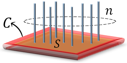
The Wilson surface whose boundary is the Wilson loop is not unique and different Wilson surfaces are related to each other by gauge transformations. On the other hand, the string tension which is calculated by the Wilson loop average, is a gauge invariant quantity and is independent of the choice of the Wilson surface shape. Each point on the Wilson surface is characterized by $\left(t,x,y\right)$. For simplicity, we consider the Wilson surface as a rectangular shape on the $t-x$ plane and each point on this Wilson surface is parameterized by $\left(\bar{t},\bar{x}\right)$. Fig. 4 shows a schematic picture of a three dimensional Wilson loop which is projected on $t-x$ plane. The origin is located on one of the corners of the rectangle. Projection on the $t-x$ plane is assumed to be equivalent to a gauge transformation.

Figure 4: Intersection between the Wilson surface and the vortex loop.

Replacing Eqs. (15) and (47) in Eq. (62),

$$\begin{split}I_{2}&=e^{-\frac{v^{2}\nu^{2}}{12\kappa}\int_{S}d^{2}\sigma_{\mu}\int_{S}d^{2}\sigma^{\prime}_{\mu}\int d^{3}x\delta^{\left(3\right)}\left(x-\bar{x}(\sigma)\right)\delta^{\left(3\right)}\left(x-\bar{x}^{\prime}(\sigma^{\prime})\right)}\\ &=e^{-\frac{v^{2}\nu^{2}}{12\kappa}\int_{S}d^{2}\sigma_{\mu}\int_{S}d^{2}\sigma^{\prime}_{\mu}\delta^{\left(3\right)}\left(\bar{x}^{\prime}(\sigma^{\prime})-\bar{x}(\sigma)\right)}\\ &=e^{-\frac{v^{2}\nu^{2}}{12\kappa}\int_{S}d^{2}\sigma_{\mu}\int_{S}d\bar{t}^{\prime}d\bar{x}^{\prime}\delta\left(\bar{t}^{\prime}-\bar{t}\right)\delta\left(\bar{x}^{\prime}-\bar{x}\right)\delta\left(\bar{y}^{\prime}-\bar{y}\right)}\\ &=e^{-\frac{v^{2}\nu^{2}}{12\kappa}\int_{S}d\bar{t}d\bar{x}\delta\left(\bar{y}^{\prime}-\bar{y}\right)}.\end{split}$$ (63)

We have chosen $\bar{y}^{\prime}=0$ since the projected Wilson loop is indeed located at the $t-x$ plane. Therefore the above equation is,

$$I_{2}=e^{-\frac{v^{2}\nu^{2}}{12\kappa}\delta\left(\bar{y}\right)\int_{0}^{\tau}d\bar{t}\int_{0}^{l_{x}}d\bar{x}}=e^{-\frac{v^{2}\nu^{2}}{12\kappa}\delta\left(\bar{y}\right)\times S},$$ (64)

where $S\equiv\tau l_{x}$ is the area of the Wilson loop in the $t-x$ plane. $\delta\left(\bar{y}\right)$ shows the intersection location of the Wilson surface and the vortex loop (see Fig. 1.(c)). In other words, we have a singularity at $\bar{y}=0$.

The third exponential function of the integral of Eq. (60) is,

$$I_{3}\equiv e^{\frac{i}{3\kappa}\int d^{3}x\left(\partial_{\mu}\bar{V}(x)\right)J^{C}_{\mu}V(x)}.$$ (65)

Replacing Eqs. (15) and (47) in Eq. (65),

$$\begin{split}I_{3}&=e^{\frac{i}{3\kappa}\int d^{3}x\partial_{\mu}\left(ve^{-i\gamma(x)}\right)\frac{\nu}{2}\int_{S}d^{2}\sigma_{\mu}\delta^{\left(3\right)}\left(x-\bar{x}(\sigma)\right)ve^{i\gamma(x)}}\\ &=e^{\frac{v^{2}\nu}{6\kappa}\int_{S}d^{2}\sigma_{\mu}\int d^{3}x\partial_{\mu}\gamma(x)\delta^{\left(3\right)}\left(x-\bar{x}(\sigma)\right)}\\ &=e^{\frac{v^{2}\nu}{6\kappa}\int_{S}d^{2}\sigma_{\mu}\partial_{\mu}\gamma(\bar{x}(\sigma))}.\end{split}$$ (66)

On the other hand,

$$d^{2}\sigma_{\mu}\partial_{\mu}\gamma(x(\sigma))=d^{2}\sigma_{0}\partial_{0}\gamma(x)+d^{2}\sigma_{1}\partial_{1}\gamma(x)+d^{2}\sigma_{2}\partial_{2}\gamma(x).$$ (67)

From Fig. (4), we choose the following parameterization,

$$\begin{split}&\bar{x}_{0}=\bar{t},\quad\bar{x}_{1}=\bar{x},\quad\bar{x}_{2}=\bar{y}\\ &\sigma_{1}=\bar{t},\quad\sigma_{2}=\bar{x}.\end{split}$$ (68)

Using Eqs. (13) and (68), the surface elements $d^{2}\sigma_{0}$ and $d^{2}\sigma_{1}$ are zero, and the surface element $d^{2}\sigma_{2}$ is equal to $d\bar{t}d\bar{x}$. Thus,

$$d^{2}\sigma_{\mu}\partial_{\mu}\gamma(x(\sigma))=d^{2}\sigma_{2}\partial_{2}\gamma(x(\sigma))=d\bar{t}d\bar{x}\dfrac{\partial\gamma(x)}{\partial y}.$$ (69)

From Eq. (55),

$$\begin{split}&\dfrac{\partial\gamma(x)}{\partial y}=\sum_{n=-\infty}^{\infty}\sum_{\vec{p}}ip_{y}\ e^{i\left(w_{n}t+\vec{p}.\vec{x}\right)}\gamma_{n}(\vec{p}),\\ &\dfrac{\partial\gamma(\bar{x})}{\partial y}\mid_{S}=\sum_{n=-\infty}^{\infty}\sum_{\vec{p}}ip_{y}\ e^{i\left(w_{n}\bar{t}+p_{x}\bar{x}\right)}\gamma_{n}(\vec{p}).\end{split}$$ (70)

Finally,

$$\int_{S}d^{2}\sigma_{\mu}\partial_{\mu}\gamma(\bar{x}(\sigma))=\sum_{n=-\infty}^{\infty}\sum_{\vec{p}}ip_{y}\gamma_{n}(\vec{p})\int_{S}d\bar{t}d\bar{x}e^{i\left(w_{n}\bar{t}+p_{x}\bar{x}\right)}.$$ (71)

Replacing Eq. (71) in Eq. (66),

$$\begin{split}I_{3}&=e^{\frac{v^{2}\nu}{6\kappa}\sum_{n=-\infty}^{\infty}\sum_{\vec{p}}ip_{y}\gamma_{n}(\vec{p})\int_{0}^{\tau}d\bar{t}e^{iw_{n}\bar{t}}\int_{0}^{l_{x}}d\bar{x}e^{ip_{x}\bar{x}}}\\ &=e^{\frac{v^{2}\nu}{6\kappa}\sum_{n=-\infty}^{\infty}\sum_{\vec{p}}ip_{y}\gamma_{n}(\vec{p})\tau l_{x}\delta_{w_{n},0}\delta_{p_{x},0}},\end{split}$$ (72)

where $w_{n}=2\pi nT$. Therefore, for finite temperature $\delta_{w_{n},0}=\delta_{n,0}$.

$$I_{3}=e^{i\frac{v^{2}\nu}{6\kappa}\tau l_{x}\sum_{\vec{p}}p_{y}\gamma_{0}\left(\vec{\mathtt{P}}\right)}=\prod_{\vec{p}}e^{i\frac{v^{2}\nu}{6\kappa}\tau l_{x}p_{y}\gamma_{0}\left(\vec{\mathtt{P}}\right)},$$ (73)

where, we define $\gamma_{0}\left(\vec{\mathtt{P}}\right)\equiv\gamma_{0}\left(0,\vec{p}_{y}\right)$.

The fourth exponential of the integral of Eq. (60) is,

$$I_{4}\equiv e^{-\frac{i}{3\kappa}\int d^{3}xJ^{C}_{\mu}(x)\bar{V}(x)\partial_{\mu}V(x)}.$$ (74)

Replacing Eqs. (15) and (47) in Eq. (74),

$$\begin{split}I_{4}&=e^{-\frac{i}{3\kappa}\int d^{3}x\frac{\nu}{2}\int_{S}d^{2}\sigma_{\mu}\delta^{\left(3\right)}\left(x-\bar{x}(\sigma)\right)ve^{-i\gamma(x)}\partial_{\mu}\left(ve^{i\gamma(x)}\right)}\\ &=e^{\frac{v^{2}\nu}{6\kappa}\int_{S}d^{2}\sigma_{\mu}\partial_{\mu}\gamma(\bar{x}(\sigma))}.\end{split}$$ (75)

Comparing Eqs. (66) and (75), we conclude that $I_{3}=I_{4}$.

Now we are ready to calculate the partition function for the linking Wilson loop and vortices using the above calculations. Replacing Eqs. (61), (64) and (73) in Eq. (60),

$$\begin{split}Z\left[J^{C}_{\mu}\right]&=N^{\prime}v^{2}e^{-\frac{v^{2}\nu^{2}}{12\kappa}\delta\left(\bar{y}\right)\times S}\prod_{n=-\infty}^{\infty}\prod_{\vec{p}}\int d\gamma_{n}(\vec{p})\ e^{-\frac{v^{2}\mathtt{V}}{3\kappa}\left(w_{n}^{2}+\vec{p}^{2}\right)\left|\gamma_{n}(\vec{p})\right|^{2}}e^{i\frac{v^{2}\nu}{3\kappa}\tau l_{x}p_{y}\gamma_{0}\left(\vec{\mathtt{P}}\right)}\\ &=N^{\prime}v^{2}e^{-\frac{v^{2}\nu^{2}}{12\kappa}\delta\left(\bar{y}\right)\times S}\times\left\{\prod_{\overset{n=-\infty}{n\neq 0}}^{\infty}\prod_{\overset{\vec{p}}{p_{x}\neq 0}}\int d\gamma_{n}(\vec{p})\ e^{-\frac{v^{2}\mathtt{V}}{3\kappa}\left(w_{n}^{2}+\vec{p}^{2}\right)\left|\gamma_{n}(\vec{p})\right|^{2}}\right\}\\ &\qquad\qquad\quad\quad\quad\quad\quad\times\left\{\prod_{\overset{\vec{p}}{p_{x}=0}}\int d\gamma_{0}\left(\vec{\mathtt{p}}\right)e^{\left[-\frac{v^{2}\mathtt{V}}{3\kappa}p^{2}_{y}\left|\gamma_{0}(\vec{\mathtt{P}})\right|^{2}+i\frac{v^{2}\nu}{3\kappa}\tau l_{x}p_{y}\gamma_{0}\left(\vec{\mathtt{P}}\right)\right]}\right\}.\end{split}$$ (76)

Using the Gaussian formula

$$Z\left[J^{C}_{\mu}\right]=N^{\prime}v^{2}e^{-\frac{v^{2}\nu^{2}}{12\kappa}\delta\left(\bar{y}\right)\times S}\times\left\{\prod_{\overset{n=-\infty}{n\neq 0}}^{\infty}\prod_{\overset{\vec{p}}{p_{x}\neq 0}}\left(\dfrac{3\kappa\pi}{v^{2}\mathtt{V}}\right)^{\frac{1}{2}}\left[w_{n}^{2}+\vec{p}^{2}\right]^{-\frac{1}{2}}\right\}\times\left\{\prod_{\overset{\vec{p}}{p_{x}=0}}\left(\dfrac{3\kappa\pi}{v^{2}\mathtt{V}}\right)^{\frac{1}{2}}\dfrac{1}{p_{y}}\right\}\times e^{-\frac{v^{2}\nu^{2}}{12\kappa}\ \frac{\tau^{2}l^{2}_{x}}{\mathtt{V}}}.$$ (77)

Following the same method of calculation $Z[J^{C}_{\mu}]$, we obtain $Z[0]$ from Eq. (58),

$$\begin{split}Z[0]&=N^{\prime}v^{2}\prod_{n=-\infty}^{\infty}\prod_{\vec{p}}\ \int d\gamma_{n}(\vec{p})\ e^{-\frac{v^{2}\mathtt{V}}{3\kappa}\left(w_{n}^{2}+\vec{p}^{2}\right)\left|\gamma_{n}(\vec{p})\right|^{2}}\\ &=N^{\prime}v^{2}\left\{\prod_{\overset{n=-\infty}{n\neq 0}}^{\infty}\prod_{\overset{\vec{p}}{p_{x}\neq 0}}\int d\gamma_{n}(\vec{p})e^{-\frac{v^{2}\mathtt{V}}{3\kappa}\left(w_{n}^{2}+\vec{p}^{2}\right)\left|\gamma_{n}(\vec{p})\right|^{2}}\right\}\times\left\{\prod_{\overset{\vec{p}}{p_{x}=0}}d\gamma_{0}(\vec{\mathtt{P}})e^{-\frac{v^{2}\mathtt{V}p^{2}_{y}}{3\kappa}\left|\gamma_{0}(\vec{\mathtt{P}})\right|^{2}}\right\}\\ &=N^{\prime}v^{2}\left\{\prod_{\overset{n=-\infty}{n\neq 0}}^{\infty}\prod_{\overset{\vec{p}}{p_{x}\neq 0}}\left(\dfrac{3\kappa\pi}{v^{2}\mathtt{V}}\right)^{\dfrac{1}{2}}\left[w_{n}^{2}+\vec{p}^{2}\right]^{-\dfrac{1}{2}}\right\}\times\left\{\prod_{\overset{\vec{p}}{p_{x}=0}}\left(\dfrac{3\kappa\pi}{v^{2}\mathtt{V}}\right)^{\dfrac{1}{2}}\dfrac{1}{p_{y}}\right\}.\end{split}$$ (78)

Next, we compute the Wilson loop average for the vortex ensemble by replacing Eqs. (77) and (78) in Eq. (50),

$$\begin{split}\left\langle W(C)\right\rangle&=\dfrac{N^{\prime}v^{2}e^{-\frac{v^{2}\nu^{2}}{12\kappa}\delta\left(\bar{y}\right)\times S}\times\left\{\prod_{\overset{n=-\infty}{n\neq 0}}^{\infty}\prod_{\overset{\vec{p}}{p_{x}\neq 0}}\left(\dfrac{3\kappa\pi}{v^{2}\mathtt{V}}\right)^{\frac{1}{2}}\left[w_{n}^{2}+\vec{p}^{2}\right]^{-\frac{1}{2}}\right\}\times\left\{\prod_{\overset{\vec{p}}{p_{x}=0}}\left(\dfrac{3\kappa\pi}{v^{2}\mathtt{V}}\right)^{\frac{1}{2}}\dfrac{1}{p_{y}}\right\}\times e^{-\frac{v^{2}\nu^{2}}{12\kappa}\ \frac{\tau^{2}l^{2}_{x}}{\mathtt{V}}}}{N^{\prime}v^{2}\left\{\prod_{\overset{n=-\infty}{n\neq 0}}^{\infty}\prod_{\overset{\vec{p}}{p_{x}\neq 0}}\left(\dfrac{3\kappa\pi}{v^{2}\mathtt{V}}\right)^{\frac{1}{2}}\left[w_{n}^{2}+\vec{p}^{2}\right]^{-\frac{1}{2}}\right\}\times\left\{\prod_{\overset{\vec{p}}{p_{x}=0}}\left(\dfrac{3\kappa\pi}{v^{2}\mathtt{V}}\right)^{\frac{1}{2}}\dfrac{1}{p_{y}}\right\}}\\ \\ &=e^{-\frac{v^{2}\nu^{2}}{12\kappa}\delta\left(\bar{y}\right)\times S}\times e^{-\frac{v^{2}\nu^{2}}{12\kappa}\ \frac{\tau^{2}l^{2}_{x}}{\mathtt{V}}}.\end{split}$$ (79)

In the infinite-volume limit, the second exponential in Eq. (79) is,

$$\lim_{\mathtt{V}\rightarrow\infty}e^{-\frac{v^{2}\nu^{2}}{12\kappa}\ \frac{\tau^{2}l^{2}_{x}}{\mathtt{V}}}=1.$$ (80)

Then, simplifying Eq. (79), the Wilson loop average $\left\langle W(C)\right\rangle$ is obtained,

$$\left\langle W(C)\right\rangle=e^{-\frac{v^{2}\nu^{2}}{12\kappa}\delta\left(\bar{y}\right)\times S}.$$ (81)

This is what we have planned to obtain, the area law fall-off for the Wilson loop which corresponds to a linear potential between a pair of static quark-antiquark.

Next, we obtain the string tension and discuss its characteristics in terms of the stiffness, tension and the parameter defined as the potential strength between the vortices. As mentioned in section II, when a Wilson loop pierces the hypersurface $\Sigma$, it observes a singularity (see Fig. 1.(a)), which multiplies the Wilson loop by a phase (see Eq. (1)). On the other hand, we recall that the linking number $L\left(C,l\right)$ is symmetric concerning the interchange of the loops $C$ and $l$. Therefore, it can be interpreted in such a way that the Wilson surface $S$ pierces by the vortex loop $l$ and the singularity on $S$ is observed (see Fig. 1.(c)). This singularity is shown as $\delta(\bar{y})$ in Eq. (81). For simplicity, we consider the Wilson surface as a rectangular shape on the $t-x$ plane, therefore this singularity is located on the $\bar{y}=0$ plane.

The area $S$ and the string tension $\sigma$ have dimensions $L^{2}$ and $L^{-2}$, respectively; where $L$ indicates the length. On the other hand, the delta function $\delta(\bar{y})$ has dimension $L^{-1}$. Using temperature $T$ which has dimension $L^{-1}$, the Wilson loop is rewritten as,

$$\left\langle W(C)\right\rangle=e^{-\frac{v^{2}\nu^{2}T}{12\kappa}\frac{\delta\left(\bar{y}\right)}{T}\times S}.$$ (82)

Where the parameter $\dfrac{\delta(\bar{y})}{T}$ is dimensionless. As a result, the string tension is obtained in terms of the parameters $v$, $\nu$ and $\dfrac{1}{\kappa}$ which are the vacuum expectation value, the co-weights and stiffness, respectively,

$$\sigma=\dfrac{v^{2}\nu^{2}}{12\kappa}T.$$ (83)

Using Eq. (46) and the fact that for the fundamental representation $\nu=\dfrac{1}{2}$, the string tension of Eq. (83) is obtained as the following,

$$\sigma=\dfrac{\left|\mu\right|\zeta}{48\kappa}T.$$ (84)

Where the sign of $\mu$ is applied by using the absolute value in the above equation. Since all the parameters $\mu$, $\zeta$, $\kappa$ and $T$ have dimension $L^{-1}$, the string tension in Eq. (84) has dimension $L^{-2}$.

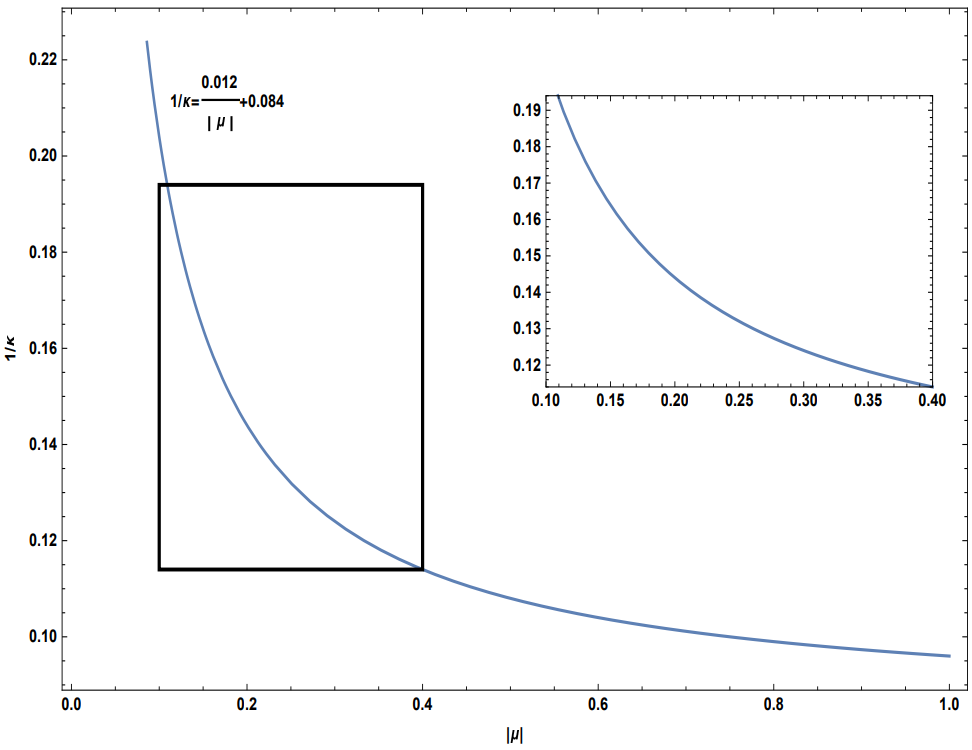
From Eq. (84), the relation between the tension $\left|\mu\right|$ and the stiffness $\dfrac{1}{\kappa}$ is,

$$\dfrac{1}{\kappa}=\dfrac{48\sigma}{\zeta T}\dfrac{1}{\left|\mu\right|}.$$ (85)

This equation shows that the stiffness $\dfrac{1}{\kappa}$ decreases by increasing the tension $\left|\mu\right|$. Reduction of the stiffness results in a more flexible vortex loop. This behavior is in good qualitative agreement with the results reported in stiff1 .

To plot the stiffness $\dfrac{1}{\kappa}$ versus the tension $\left|\mu\right|$, one must know the coefficient $\dfrac{48\sigma}{\zeta T}$ in Eq. (85). We have used figure $2$ of reference stiff1 and the coefficient is obtained to be approximately equal to 0.012. Fig. 5 shows the plot of $\dfrac{1}{\kappa}$ versus $\left|\mu\right|$ from our calculation and using the coefficient $\dfrac{48\sigma}{\zeta T}$ obtained from reference stiff1 . The stiffness and the tension are scaled with the temperature and are dimensionless. A magnification is done in the upper right to compare the data with the range of the data reported in figure 2 of reference stiff1 .

Assuming $\dfrac{48\sigma}{\zeta T}=0.012$ from the above discussion, the dimensionless string tension is rewritten from Eq. (85),

$$\dfrac{\sigma(T)}{T^{2}}=\dfrac{0.012}{48}\dfrac{\zeta(T)}{T}.$$ (86)

Figure 5: stiffness $\dfrac{1}{\kappa}$ versus the tension $\left|\mu\right|$. A magnification is done in the upper right of the plot to compare the data with the range of the data reported in ref. stiff1 .

On the other hand, the temperature dependence of SU($2$) string tension has been computed by lattice QCD zeta ,

$$\dfrac{\sigma(T)}{T^{2}}=\dfrac{\sigma_{0}}{T^{2}_{c}}\left(\dfrac{T_{c}}{T}\right)^{2}A\left(1-\dfrac{T}{T_{c}}\right)^{0.63}\left(1+B\left(1-\dfrac{T}{T_{c}}\right)^{\frac{1}{2}}\right),$$ (87)

where the constants $A=1.39$ and $B=\dfrac{1}{A}-1$ zeta . The ratio $\dfrac{T_{c}}{\sqrt{\sigma_{0}}}\approx 0.69$ with $\sigma_{0}=\left(440\text{Mev}\right)^{2}$ stiff1 , gives $T_{c}=303.6\text{Mev}$. From Eqs. (86) and (87), the dimensionless quantity $\dfrac{\zeta(T)}{T}$ is concluded,

$$\dfrac{\zeta(T)}{T}=\dfrac{48}{0.012}\dfrac{\sigma_{0}}{T^{2}}A\left(1-\dfrac{T}{T_{c}}\right)^{0.63}\left(1+B\left(1-\dfrac{T}{T_{c}}\right)^{\frac{1}{2}}\right),$$ (88)

where the string tension and $\dfrac{\zeta(T)}{T}$ are scaled with the temperature. Fig. 6 plots $\dfrac{1}{\zeta(T)}$ versus $\dfrac{T}{T_{c}}$.

Figure 6: Dependence of the parameter which indicates the potential strength between the vortices, to the temperature.

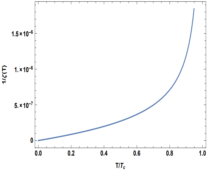
The potential between the vortices represented in Eq. (21) is repulsive and it is a function of the parameter $\dfrac{1}{\zeta}$. On the other hand, Fig. 6 shows that $\dfrac{1}{\zeta}$ increases by increasing the temperature. Thus, the repulsive potential between the vortices increases by increasing the temperature. This result is in good agreement with the result of lattice QCD zeta lattice and the fact that by increasing the temperature one gets close to the deconfinement regime and expects the disappearance of vortex configurations. Increasing the repulsive forces between the vortices at higher temperatures may prevent the vortices from having stable topological structures required for quark confinement.

V Summary and Conclusions

Inspired by lattice results confirming the area law fall-off for the Wilson loop average, we compute the Wilson loop in the continuum limit for SU($2$) gauge group in three-dimensional Euclidean space-time. The area law fall-off is observed and the linear potential between a pair of quark-antiquark and the string tension is obtained.

A technique used by polymer physicists and later by particle physicists is applied to an ensemble of vortices to get the appropriate partition function containing a free complex scalar field representing the vortex field. The action of an ensemble of $n$ non-interacting vortices is written in terms of two intrinsic parameters of the vortices called the tension and the stiffness. Then, a potential between the vortices is assumed and the partition function of the ensemble of vortices linking the Wilson loop, is obtained.

We have used the above partition function to compute the Wilson loop. The area law fall-off for the Wilson loop is observed and the string tension is extracted in terms of the vortices parameters. The stiffens versus the tension plot of this calculation is in good qualitative agreement with the lattice results reported by stiff1 .

A comparison between our results and the lattice ones stiff1 is done to obtain a coefficient of our calculations which contains the string tension and the potential strength. As a result, a dimensionless string tension is defined in terms of the potential strength. This string tension is compared with the string tension reported by zeta , and the potential strength in terms of the temperature is obtained. It is shown that the repulsive force between the vortices increases with the temperature. This is what one expects from the vortex models if one wants to see the reduction of vortex effects at higher temperatures. It is also in agreement with lattice results where the effect of topological defects must be decreased at smaller distances.

References

• (1) R. F. Alvarez-Estrada, F. Fernandez, J. L. Sanchez-Gomez, and V. Vento, Models of Hadrons Structure Based on Quantum Chromodynamics (Springer, Berlin, Heidelberg, 1986).
• (2) W. Greiner, S. Schramm, E. Stein, and D.A. Bromley, Quantum Chromodynamics (Springer, 2004).
• (3) C. Gattringe, and C. B. Lang,Quantum Chromodynamics on the Lattice: On Introductory Presentation (Springer-Varlag, Berlin, Heidelberg, 2010).
• (4) C.N. Yang, and R.L. Mills, Conservation of isotopic spin and isotopic gauge invariance, Phys. Rev. 96, 191 (1954).
• (5) W. Marciano, and H. Pagels, Quantum chromodynamics: A review. Phys. Rep. 36, 137 (1978).
• (6) Y. Nambu, and G. Jona-Lasinio, Dynamical model of elementary particles based on an analogy with superconductivity. I, Phys. Rev. 122, 345 (1961).
• (7) Y. Nambu, and G. Jona-Lasinio, Dynamical model of elementary particles based on an analogy with superconductivity. II, Phys. Rev. 124, 246 (1961).
• (8) K. Higashijima, Theory of Dynamical Symmetry Breaking, Prog. Theor. Phys. Suppl. 104, 1 (1991).
• (9) U. Bar-Gadda, Infrared behavior of the effective coupling in quantum Chromodynamics: a non-perturbative approach, Nucl. Phys. B163, 312 (1980).
• (10) E. V. Shuryak, Theory and phenomenology of the QCD vacuum, Phys. Rep. 115, 151 (1984).
• (11) D. I. Diakonov, and V. Yu. Petrov, A theory of light quarks in the instanton vacuum, Nucl. Phys. B272, 457 (1986).
• (12) H. Suganuma, N. Ishii, M. Oka, H. Enyo, T. Hatsuda, T. Kunihiro, and K. Yazaki, International Conference on Color Confinement and Hadrons in Quantum Chromodynamics: The Institute of Physical and Chemical Research (World Scientific, Singapore, 2004).
• (13) J. Greensite, An Introduction to the Confinement Problem (Lecture Notes in Physics) (Springer-Varlag, Berlin, Heidelberg, 2011).
• (14) Y. M. Cho, Restricted gauge theory, Phys. Rev. D 21, 1080 (1980).
• (15) Y. M. Cho, Extended gauge theory and its mass spectrum, Phys. Rev. D 23, 2415 (1981).
• (16) L. Faddeev, and A. J. Niemi, Partially dual variables in SU($2$) Yang-Mills theory, Phys. Rev. Lett. 82, 1624 (1999).
• (17) G. ’t Hooft, On the phase transition towards permanent quark confinement, Nucl.Phys. B138, 1 (1978).
• (18) J. M. Cornwall, Quark confinement and vortices in massive gauge invariant QCD, Nucl. Phys. B157, 392 (1979).
• (19) G. ’t Hooft, Confinement and topology in non-Abelian gauge theories, Austriaca Suppl. 22, 531 (1980).
• (20) G. ‘t Hooft, Topology of the gauge condition and new confinement phases in non-Abelian gauge theories, Nucl. Phys. B190, 455 (1981).
• (21) G. ‘t Hooft, The topological mechanism for permanent quark confinement in a non-Abelian gauge theory, Phys. Scr. 25, 133 (1982).
• (22) S.V. Shabanov, Yang-Mills theory as an Abelian theory without gauge fixing, Phys. Lett. B 463, 263 (1999).
• (23) L. Faddeev, and A.J. Niemi, Decomposing the Yang-Mills field, Phys. Lett. B 464, 90 (1999).
• (24) G. Ripka, Dual superconductor models of color confinement, Lect. Notes Phys. 639, 1 (2004).
• (25) H. Ichie, and H. Suganuma, Dual Higgs theory for color confinement in quantum Chromodynamics, arXiv: hep-lat/9906005.
• (26) J. D. Stack, S. D. Neiman, and R. Wensley, String tension from monopoles in SU($2$) lattice gauge theory, Phys. Rev. D 50, 3399 (1994).
• (27) R. W. Haymaker, Confinement studies in lattice QCD, Phys. Rep. 315, 153 (1999).
• (28) K.-I. Kondo, and Y. Taira, A proposal of lattice simulation for quark confinement based on a novel reformulation of QCD, Nucl. Phys. Proc. Suppl. 83, 497 (2000).
• (29) L. Dittmann, T. Heinzl, and A. Wipf, A lattice study of the Faddeev-Niemi effective action, Nucl. Phys. Proc. Suppl. 106, 649 (2002).
• (30) J. Greensite, The confinement problem in lattice gauge theory, Prog. Part. Nucl. Phys. 51, 1 (2003).
• (31) S. Kato, K.-I. Kondo, T. Murakami, A. Shibata, T. Shinohara, and S. Ito, Lattice construction of Cho–Faddeev–Niemi decomposition and gauge invariant monopole, Phys. Lett. B 632, 326 (2006).
• (32) S. Ito, S. Kato, K.-I. Kondo, T. Murakami, A. Shibata, and T. Shinohara, Compact lattice formulation of Cho-Faddeev-Niemi decomposition: String tension from magnetic monopoles, Phys. Lett. B 645, 67 (2007).
• (33) K.-I. Kondo, A. Shibata, T. Shinohara, T. Murakami, S. Kato, and S. Ito, New descriptions of lattice SU($N$) Yang-Mills theory towards quark confinement, Phys. Lett. B 669, 107 (2008).
• (34) S. Kato, K.-I. Kondo, and A. Shibata, Gauge-independent “Abelian” and magnetic-monopole dominance, and the dual Meissner effect in lattice SU($2$) Yang-Mills theory, Phys. Rev. D 91, 034506 (2015).
• (35) H. J. Rothe, Lattice Gauge Theories: An introduction (World Scientific Lecture Notes in Physics), 4th edition (World Scientific, 2012).
• (36) S. M. Hosseini Nejad, and S. Deldar, Role of the SU($2$) and SU($3$) subgroups in observing confinement in the G($2$) gauge group, Phys.Rev.D 89, 1 (2014).
• (37) S. Deldar, and A. Mohamadnejad, Quark confinement in restricted SU($2$) Gauge Theory, Phys. Rev. D 86, 065005 (2012).
• (38) F. Bruckmann, Topological objects in QCD, JHEP 152, 61 (2007).
• (39) A. Mohamadnejad, and S. Deldar, Appearance of vortices and monopoles in a decomposition of an SU($2$) Yang–Mills field, PTEP 2015, 2 (2015).
• (40) Z. Dehghan, and S. Deldar, Cho decomposition, Abelian gauge fixing, and monopoles in G($2$) Yang-Mills theory, Phys.Rev.D 99, 11 (2019).
• (41) N. Karimimanesh, and S. Deldar, Detection of monopoles and vortices in SU($2$) Yang–Mills theory, Int.J.Mod.Phys.A 37, 1 (2022).
• (42) K.-I. Kondo, S.Kato, A. Shibata, and T. Shinohara, Quark confinement: Dual superconductor picture based on a non-Abelian Stokes theorem and reformulations of Yang-Mills theory, Phys. Rep. 579, 1 (2015).
• (43) T. Appelquist, M. Dine, and I. J. Muzinich, The static potential in quantum chromodynamics, Phys. Lett. B 69, 231 (1977).
• (44) K. Wilson, Confinement of quarks, Phys. Rev. D 10, 2445 (1974).
• (45) L. P. Gor’kov, Microscopic derivation of the Ginzburg-Landau equations in the theory of superconductivity, Sov. Phys. JETP 9, 1364 (1959).
• (46) A. A. Abrikosov, Nobel lecture: Type-II superconductors and the vortex lattice, Rev. Mod. Phys. 76, 975 (2004).
• (47) H. B. Nielsen, and P. Olesen, A quantum liquid model for the QCD vacuum: Gauge and rotational invariance of domain and quantized homogeneous color fields, Nucl. Phys. B160, 380 (1979).
• (48) J. Ambjorn, and P. Olesen, On the formation of a random color magnetic quantum liquid in QCD, Nucl. Phys. B170, 60 (1980).
• (49) G. Mack, Predictions of a Theory of Quark Confinement, Phys. Rev. Lett. 45, 1378 (1980).
• (50) G. Mack, and V.B. Petkova, Sufficient condition for confinement of static quarks by a vortex condensation mechanism, Ann. Phys. (N. Y.) 125, 117 (1980).
• (51) L. D. Debbio, M. Faber, J. Greensite, and S. Olejnik, Center dominance and Z($2$) vortices in SU($2$) lattice gauge theory, Phys. Rev. D 55, 2298 (1997).
• (52) L. D. Debbio, M. Faber, J. Giedt, J. Greensite, and S. Olejnik, Detection of center vortices in the lattice Yang-Mills vacuum, Phys. Rev. D 58, 094501 (1998).
• (53) L. D. Debbio, M. Faber, J. Greensite, and S. Olejnik, Some cautionary remarks on Abelian projection and Abelian dominance, Nucl. Phys. Proc. Suppl. 53, 141 (1997).
• (54) K. Langfeld, O. Tennert, M. Engelhardt, and H. Reinhardt, Center vortices of Yang-Mills theory at finite temperatures, Phys. Lett. B 452, 301 (1999).
• (55) M. Engelhardt, K. Langfeld, H. Reinhardt, and O. Tennert, Deconfinement in SU($2$) Yang-Mills theory as a center vortex percolation transition, Phys. Rev. D 61, 054504 (2000).
• (56) J. Gattnar, K. Langfeld, and H. Reinhardt, Center-vortex dominance after dimensional reduction of SU($2$) lattice gauge theory, Phys. Lett. B 489, 251 (2000).
• (57) K. Langfeld, Vortex structures in pure lattice gauge theory, Phys. Rev. D 69, 014503 (2004).
• (58) M. Faber, J. Greensite, and S. Olejnik, Casimir scaling from center vortices: Towards an understanding of the adjoint string tension, Phys. Rev. D 57, 2603 (1998).
• (59) L. D. Debbio, M. Faber, J. Greensite, and S. Olejnik, Center dominance, center vortices, and confinement, arXiv:hep-lat/9708023.
• (60) S. Deldar, Potentials between static SU($3$) sources in the fat center vortices model, JHEP 01, 013 (2001).
• (61) S. Deldar, and Sh. Rafibakhsh, SU($4$) string tensions from the fat-center-vortices model, JHEP 42, 319 (2005).
• (62) S. Samuel, Topological symmetry breakdown and quark confinement, Nucl. Phys. B154, 62 (1979).
• (63) Z. Asmaee, S. Deldar, and M. Kiamari, Introducing vortices in the continuum using direct and indirect methods, Phys. Rev. D 105, 096020 (2022).
• (64) N. Karimimanesh, S. Deldar, and Z. Asmaee, Monopoles, vortices and their correlations in SU(3) gauge group, Eur. Phys. J. C 83, 483 (2023).
• (65) M. Stone, and P. R. Thomas, Condensed monopoles and Abelian confinement, Phys. Rev. Lett. 41, 351 (1978).
• (66) P. R. Thomas, and M. Stone, Nature of the Phase Transition in a Nonlinear O($2$)-$3$ Model, Nucl. Phys. B144, 513 (1978).
• (67) K. Bardakci, and S. Samuel, Local field theory for solitons, Phys. Rev. D 18, 2849 (1978).
• (68) L. E. Oxman, and H. Reinhardt, Effective theory of the D $=3$ center vortex ensemble, Eur. Phys. J. C 78, 3 (2018).
• (69) C. Alexandrou, P. de Forcrand, and M. D’Elia, The role of center vortices in QCD, Nucl. Phys. A663, 1031 (2000).
• (70) P. de Forcrand, and M. Pepe, Center vortices and monopoles without lattice gribov copies, Nucl. Phys. B598, 557 (2001).
• (71) K. Langfeld, and H. Reinhardt, Center vortex properties in the Laplace center gauge of SU($2$) Yang-Mills theory, Phys. Lett. B 504, 338 (2001).
• (72) M. Faber, J. Greensite, and S. Olejnik, Direct Laplacian center gauge, JHEP 11, 53 (2001).
• (73) M. Engelhardt, and H. Reinhardt, Center projection vortices in continuum Yang-Mills theory, Nucl. Phys. B567, 249 (2000).
• (74) M. Engelhardt, and H. Reinhardt, Center vortex model for the infrared sector of Yang-Mills theory - Confinement and Deconfinement, Nucl. Phys. B585, 591 (2000).
• (75) M. Engelhardt, M. Quandt, and H. Reinhardt, Center Vortex Model for the Infrared Sector of SU($3$) Yang-Mills Theory - Confinement and Deconfinement, Nucl. Phys. B685, 227 (2004).
• (76) M. Quandt, H. Reinhardt, and M. Engelhardt, Center Vortex Model for the Infrared Sector of SU(3) Yang-Mills Theory - Vortex Free Energy, Phys. Rev. D 71, 054026 (2005).
• (77) G. Fredrickson, The Equilibrium Theory of Inhomogeneous Polymers (Clarendon, Oxford, 2006).
• (78) L.E. Oxman, G.C.S. Rosa, and B.F.I. Teixeira, Coloured loops in 4D and their effective field representation, J. Phys. A47, 305401, (2014).
• (79) J. I. Kapusta, and C. Gale, Finite-temperature field theory: Principles and applications, Cambridge monographs on mathematical physics, (Cambridge university press, 2006).
• (80) F. Bruckmann, S. Dinter, E. Ilgenfritz, B. Maier, M. M¨uller-Preussker, and M. Wagner, Confining dyon gas with finite-volume effects under control, Phys. Rev. D 85, 034502 (2012).
• (81) M. Engelhardt, K. Langfeld, H. Reinhardt, and O. Tennert, Interaction of confining vortices in SU($2$) lattice gauge theory, Phys. Lett. B431, 141 (1998).