Efficient Inverse Design Optimization through Multi-fidelity Simulations, Machine Learning, and Search Space Reduction Strategies

Abstract

This paper introduces a methodology designed to augment the inverse design optimization process in scenarios constrained by limited compute, through the strategic synergy of multi-fidelity evaluations, machine learning models, and optimization algorithms. The proposed methodology is analyzed on two distinct engineering inverse design problems: airfoil inverse design and the scalar field reconstruction problem. It leverages a machine learning model trained with low-fidelity simulation data, in each optimization cycle, thereby proficiently predicting a target variable and discerning whether a high-fidelity simulation is necessitated, which notably conserves computational resources. Additionally, the machine learning model is strategically deployed prior to optimization to reduce the search space, thereby further accelerating convergence toward the optimal solution. The methodology has been employed to enhance two optimization algorithms, namely Differential Evolution and Particle Swarm Optimization. Comparative analyses illustrate performance improvements across both algorithms. Notably, this method is adeptly adaptable across any inverse design application, facilitating a harmonious synergy between a representative low-fidelity ML model, and high-fidelity simulation, and can be seamlessly applied across any variety of population-based optimization algorithms.

1 Introduction

Inverse design problems represent a frontier in the field of engineering and science, where the objective is to discover the necessary system inputs to achieve a desired known output. Rather than following the traditional forward design process–which starts with given parameters and attempts to predict the outcome–inverse design turns the procedure on its head, beginning with the desired outcome and working backward to determine the optimal parameters to realize it. Particularly in scenarios with computationally expensive or hierarchical simulations, multi-fidelity evaluations play a pivotal role, offering a trade-off between accuracy and computational cost.

The first subsection provides an overview of multi-fidelity optimization methods, machine learning approaches for inverse design, a brief summary of the machine learning (ML) enhanced framework, and the organizational structure of the manuscript. The second and third subsections offer a literature review of the two distinct problems (airfoil inverse design and scalar field reconstruction) used to investigate the proposed ML-enhanced design framework.

1.1 Machine Learning Models and Multi-fidelity Inverse Design

Multi-fidelity methods, that range from faster and approximate objective function evaluations to detailed, computationally intensive ones have been explored in-depth for optimization purposes [15]. Surrogate-based optimization techniques tailored for multi-fidelity problems offer a promising approach for system approximation with the need for high-fidelity (HF) evaluations at every single optimization cycle [14].

In the context of inverse design optimization coupled with a multi-fidelity approach, an additional layer of complexity is introduced when the target output is a distribution. Bayesian optimization methods have provided great insights in this specific domain, especially when the inverse design problem is rooted in uncertainty or when prior knowledge is available [37, 41, 47]. However, due to the curse of dimensionality, Bayesian approaches can encounter computational challenges.

Many existing methods lack the adaptability to dynamically select the appropriate fidelity level based on interim results or statistical confidence. The integration of ML tools with traditional optimization in a cohesive framework for inverse design, while also ensuring interpretability remains a nuanced challenge.

The essence of multi-fidelity (MF) simulations is to harmoniously integrate models of varying accuracy and computational expense. By leveraging the strengths of both high-fidelity (HF) and ML models, it is possible to achieve accurate solutions while conserving computational resources and minimizing energy consumption in the exascale era of computing. This is especially pivotal in scenarios where computational budgets are limited, but the accuracy cannot be compromised. Hence, this paper presents an innovative inverse design framework that integrates metaheuristic algorithms with a pre-trained reduced-order low-fidelity (LF) ML model to reduce the size of the search space, thereby accelerating the inverse design process. LF data, employed in training the ML model, originates from simulations characterized by coarse discretization. The term reduced-order pertains to the method of simplifying the training data, initially a vector of values, into a singular scalar measure. In addition, the pre-trained ML model as a part of the framework decides the need for HF simulations by comparing the discrepancy between the target performance and the predicted LF reduced-order information. This innovation stands out from prior research by facilitating predictive decision-making regarding the necessity for HF simulations, leveraging LF and reduced-order data. Once trained, the ML model can enhance optimization for any target design within its applicable domain, thereby substantially extending its reach and impact.

Within the inverse design framework, this study delves into two distinct metaheuristic population-based algorithms: Particle Swarm Optimization (PSO) and Differential Evolution (DE). It examines two separate ML algorithms and techniques for search space reduction, underscoring the framework’s modularity. Any kind of optimization algorithm could be incorporated into the framework, however, PSO and DE were chosen since they generally require a high number of evaluations. The importance of this research is emphasized by its application to airfoil inverse design and scalar field reconstruction challenges. To the best of the authors’ knowledge, no approaches in the literature combine population-based algorithms with ML techniques for both search space reduction and MF optimization within a single framework.

The manuscript is structured to offer a thorough understanding of the research. Following the introduction, Sect. 2 delves into the ML-enhanced inverse design framework. Sect. 3 and Sect. 4 provide an in-depth examination of the airfoil inverse design and the scalar field reconstruction problems, respectively. Sect. 5 outlines the numerical experiments, detailing the simulation setup, accuracy metrics, and all the hyperparameters employed in this study for both problem domains. Finally, Sect. 6 presents a comprehensive discussion of the results of the ML model, techniques for search space reduction, and a meticulous analysis of the ML-enhanced framework, contrasting it with traditional optimization algorithms.

1.2 Airfoil Inverse Design Problem

Airfoil inverse design and airfoil shape optimization occupy a pivotal role in engineering, particularly in the realm of aeronautics [4, 19] and wind energy generation [48]. The main objective is to enhance the performance of elements such as aircraft wings, wind turbine blades, or propeller blades. By optimizing the shape of an airfoil, engineers manipulate aerodynamic parameters like lift and drag, and other phenomena such as noise generation and structural stability, ultimately leading to improvements in energy consumption, speed, load-bearing capacity, and environmental impact. Airfoil inverse design, in particular, is invaluable as it allows engineers to derive the optimal shape based on desired aerodynamic properties, thereby enabling the creation of highly specialized designs tailored to specific applications or environmental conditions. This level of optimization is critical to the ongoing evolution and sustainability of technologies reliant on aerodynamic performance.

Recently, ML techniques have become dominant in the field of aerodynamic shape optimization (see the comprehensive review by Li et al [32]). More specifically, inverse design and multi-fidelity optimization approaches can be divided into two main groups: those focusing on generative models for inverse design, and those utilizing optimization methods.

In the generative models category, several researchers have applied unique methods for airfoil shape parametrization and prediction. Zhang et al [64] and Du et al [13] have developed airfoil inverse design frameworks utilizing Metric-based Proper Orthogonal Decomposition and B-Spline Generative Adversarial Network (GAN) model, respectively. Also, Xiao et al [59] used a combination of Isometric Feature Mapping, Proper Orthogonal Decomposition, and Free Form Deform method for this purpose. GANs for generating pressure distributions and shapes have been applied by Deng and Yi [10] and Wang et al [55]. Yonekura et al [62] used NACA airfoil data to train Conditional Wasserstein GAN with a gradient penalty model for generating smooth airfoil shapes. Lastly, [61] created an inverse design framework for wind airfoils based on a hybrid Multilayer Perceptron (MLP) and Variational Autoencoder.

In the optimization methods category, Du et al [12] developed a multi-fidelity manifold mapping technique for enhancing the Pattern Search algorithm. Likewise, Pehlivanoglu [42] used a continuously retrained Radial Basis Function Neural Network to accelerate the PSO process for multi-element airfoils. Other researchers like Leifsson et al [31], Koziel and Leifsson [29] focused on iterative optimization of continually corrected low-fidelity models. Furthermore, Zhu et al [65] and Lei et al [30] proposed methods to accelerate the optimization process for specific design problems such as cascaded airfoil shape and transonic wings. Han et al [19] utilized surrogate-based optimization (Kriging) for optimal shape determination. Finally, in the work by Tandis and Assareh [51], a hybrid Genetic and Bees evolutionary algorithm was developed for the inverse design of airfoils.

1.3 Scalar Field Reconstruction Problem

The scalar field reconstruction problem emerges as an inverse design challenge across various scientific and engineering domains, representing a specific variant of the inverse boundary value problem [52]. This problem centers on deducing the distribution of a scalar field from sparse measurements [3]. At its core, it entails the iterative numerical solution of the diffusion partial differential equation within the desired domain, with the ultimate goal of inversely determining the appropriate boundary condition that aligns with the target measurements.

Extracting scalar field information, especially determining boundary conditions, poses considerable challenges due to its computational intensity. Nonetheless, the need for precise reconstruction is paramount given its broad applications. These encompass environmental monitoring and pollutant dispersion [20, 60, 17], ocean remote sensing [57], thermal system studies [24], heat conduction analysis [38], material phase transitions [58], and innovations in combustion diagnostics [45, 46].

The scalar field reconstruction problem has been solved with both ML and optimization methods, however, ML approaches have been vastly more popular than optimization algorithms. In the ML approaches category, [16] developed a coupled deep reversible regression model coupled with a physics-informed approach for temperature field reconstruction. [46] used an MLP trained to reconstruct temperature and concentration fields from infrared emissions measurements. [9] created a hybrid Fruit Fly Optimization and Generalized Regression Neural Network method for fast sea salinity and temperature field reconstruction based on surface measurements. [36] utilized a Gaussian radial basis function-based kernel regression model in order to reconstruct temperature fields from acoustic signal measurements. [34] used a GAN approach to reconstruct flow fields, including temperature for a nanofluid flow case, and similarly, [35] utilized a Convolutional Neural Network for the same problem. Furthermore, Huang et al [22] utilized a hybrid Dynamic Mode Decomposition and a Convolutional Long Short-Term Memory network for temperature field reconstruction within a T-junction.

Various optimization strategies have been developed for scalar field reconstruction. These encompass the fusion of the Broyden-Fletcher-Goldfarb-Shanno algorithm with the Cuckoo Search Optimization Algorithm for transient heat conduction boundary determination [7, 6]. Genetic Algorithms have also been employed, notably in addressing the boundary conditions for material phase transitions (the Stefan boundary value problem) [49], as well as solving the inverse boundary value problem of the heat, wave, and Poisson partial differential equations [26].

The scalar reconstruction problem stands to gain substantially from the hybrid ML optimization strategy introduced in this paper. Unlike many methods discussed in this section, the approach uniquely leverages the strengths of ML in conjunction with optimization techniques. This becomes particularly valuable in adapting to large changes in the design space, a scenario where traditional ML methods might experience concept drift. In such cases, the optimization component of this strategy acts not only as a corrective measure but also as a guiding force, refining and directing the initial ML predictions towards more effective inverse design solutions.

2 ML-Enhanced Inverse Design Framework

This section introduces the ML-enhanced inverse design framework. The methodology consists of two primary stages: training an ML model and applying it to reduce the size of the search space thus enabling optimization acceleration, and finally, executing the ML-enhanced optimization process to find the design corresponding to the target performance. The framework uniquely combines LF simulation data for ML model training with HF simulations for optimization, creating a versatile multi-fidelity system. Once trained, the ML model can be utilized to augment the inverse design for a given problem. This, however, is applicable to the solutions that lie within the boundaries of the dataset used for training the model. The general workflow of the inverse design framework and the components is displayed in Fig. 1.

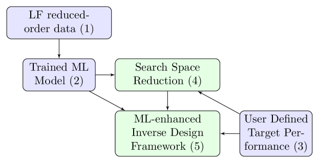
Figure 1: The training of the ML model commences with the generation of LF data (1) used for training the ML model (2). Once the model is trained and its accuracy is determined, it enables the search space reduction (4) and the ML-enhanced inverse design methodology (5). The inverse design procedure requires the specification of a target performance (3). Blocks highlighted in light green (4) and (5) denote stages involving an optimization process.

2.1 Inverse Design Optimization and Objective Function Definition

The inverse design problem can be mathematically articulated as:

$$\mathbf{x}=f^{-1}(y)$$ (1)

Here, the objective is to ascertain the design parameters $\mathbf{x}$ that generate a known target value $y$ which is evaluated with the inverse of the objective function $f$. This is in stark contrast to forward problems, where $y$ is typically unknown. Inverse design problems, tend to be ill-posed. They commonly encounter the problem of multiple viable solutions, complicating the process of identifying a unique and optimal solution.

In Eq. (2) the inverse design optimization problem is defined as:

$$\underset{\mathbf{x}}{\text{minimize}} \varepsilon(f(\mathbf{x}),y)$$ (2)

subject to $$\mathbf{x}_{lb}\leq\mathbf{x}\leq\mathbf{x}_{ub}$$

The objective of this optimization problem is to minimize the discrepancy between the desired output, $y$, and the outcome derived from the proposed design, denoted as $\mathbf{x}$. The measure of this discrepancy is given by the error-based objective function, denoted by $\varepsilon$, which can be customized to suit the unique requirements of the problem at hand. It is important to note that the design parameters $\mathbf{x}$ are not unbounded; they must lie within a compact design space defined by the lower and upper boundaries, $\mathbf{x}_{lb}$ and $\mathbf{x}_{ub}$ respectively, defined by the problem under consideration.

In this study, the root mean square error is used as $\varepsilon$:

$$\underset{\mathbf{x}}{\text{minimize}} \varepsilon(\mathbf{x})=\sqrt{\frac{1}{m}\lVert\mathbf{P}^{C}(\mathbf{x})-\mathbf{T}\rVert_{2}^{2}}$$ (3)

subject to $$\mathbf{x}_{lb}\leq\mathbf{x}\leq\mathbf{x}_{ub},$$

where x = (x₁,…, x_m)^T is the optimization design vector in the decision space $\mathbb{R}^{m}$, $m$ is the dimension of the general optimization design vector, $\mathbf{P}^{C}$$(\mathbf{x})$ denotes the computed performance based on the design vector $\mathbf{x}$, while $\mathbf{T}$ signifies the user-defined target performance. Both $\mathbf{P}^{C}$$(\mathbf{x})$ and $\mathbf{T}$ are of dimension $m$. Ideally, an exact match between these values would result in an objective function value of zero.

2.2 ML-Enhanced Optimization

The process begins by determining a target performance vector and extracting any accessible reduced-order information from it, such as statistical metrics (average, minimum, maximum, etc.), thereby defining a target performance scalar value. A prerequisite for the framework is a pre-trained ML model (discussed in Sect. 2.4), capable of predicting the reduced-order information for any design that is being evaluated during the optimization process. Furthermore, the framework utilizes an ML-generated search space reduction, thereby expediting the approximation of the optimum. Fig. 2 depicts the ML-enhanced optimization framework and all of the necessary parameters.

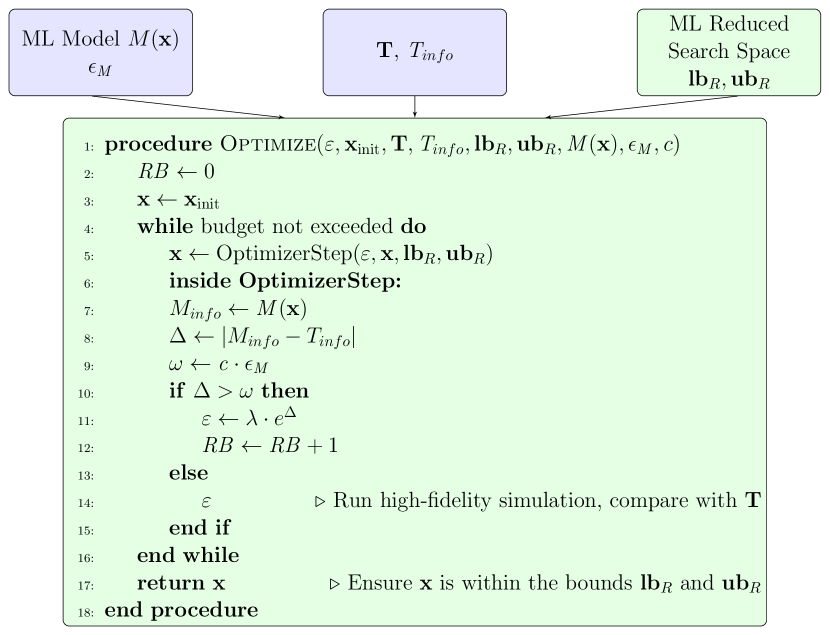
Figure 2: The flowchart and pseudo-code of the ML-enhanced inverse design framework. $\mathbf{T}$ and $\mathit{T}_{info}$ denote the user-defined target performance and the reduced-order information obtained from the target performance, respectively. $\Delta$ is the absolute error between the reduced-order target information and the ML model ($M(\mathbf{x})$) predicted reduced-order information $M_{info}$ for a given design $\mathbf{x}$. $\omega$ is the threshold parameter that is calculated by a user-defined threshold scaling factor $c$ and the error of the ML model $\epsilon_{\mathit{M}}$ (e.g. root mean square error or mean absolute error), and $\mathbf{x}_{init}$ is the initial design that was randomly generated for every optimization run. $\lambda$ denotes the error scaling parameter and is set to 2. The $\mathbf{lb}_{R}$ and $\mathbf{ub}_{R}$ denote the reduced lower and upper boundaries of the optimization design vector as defined by the ML model, respectively. Blocks highlighted in light green denote stages involving an optimization process. $RB$ denotes the remaining HF simulation budget. A higher value of $RB$ is better, and implies less HF simulations used for optimization.

During the optimization process, each evaluation of the objective function $\varepsilon$ commences with the invocation of the pre-trained ML model, denoted by $M(\mathbf{x})$ (detailed in Sect. 2.4), to predict the value of $\mathit{M}_{info}$ for a given optimization design vector $\mathbf{x}$. The subsequent step involves computing the absolute error between the ML predicted value of $\mathit{M}_{info}$ and the target value $\mathit{T}_{info}$ for each evaluation of the design vector. In cases where this predicted absolute error, designated as $\Delta$, exceeds a pre-established threshold value $\omega$, the objective function $\varepsilon$ is assigned the value of $\lambda\cdot$e^Δ ($\lambda$ = 2). Conversely, if $\Delta$ is less than or equal to $\omega$, $\varepsilon$ is evaluated with a HF simulation and a predefined error metric (Eq. (3)). The remaining budget ($RB$) denotes the remaining HF simulation budget which is used as a comparison metric with the unenhanced inverse design algorithms in Sect. 6, and a higher value of $RB$ signifies enhanced performance, specifically in terms of increased computational efficiency and savings. The optimization process stops when the simulation budget is exceeded.

The proposed ML-enhanced inverse design framework can be used in conjunction with any population-based global optimization algorithm. In this study, it is investigated how the ML model enhances two population-based algorithms, namely, DE and PSO. The fundamental goal of this framework is to enhance the robustness and efficiency of the optimization algorithms through the use of ML-generated search space reduction and ML-guided evaluation of HF simulations.

2.3 ML-Generated Search Space Reduction

Data-driven search space reduction strategies have been of interest in recent years in order to accelerate global optimization when the design space is large or when the computational budget is very limited [21, 56, 63, 43].

A pre-trained ML model is used to determine the reduced search space by minimizing the absolute difference between the target value $\mathit{T}_{info}$ and the ML-predicted value $\mathit{M}_{info}$, which are both scalar values, unlike the T which has multiple values that are compared through an appropriate error metric.

The $\mathit{T}_{info}$ value can be extracted from the T array, and it contains the same reduced-order information that the pre-trained ML model is mapped to. To determine the reduced search space, it is necessary to determine the optimal solution defined as in Eq. (4):

$$\underset{\mathbf{x}}{\text{minimize}} |\mathit{M}(\mathbf{x})-\mathit{T}_{info}|$$ (4)

subject to $$\mathbf{x}_{lb}\leq\mathbf{x}\leq\mathbf{x}_{ub}$$

The solution vector $\mathbf{x}^{*}$ represents an optimized design. The primary objective of this optimization process is to strategically reduce the search space using the ML model. This approach aims to significantly minimize the demand for computational resources, an essential factor when operating within a stringent computational budget. Given the inherent ill-posedness of most inverse design problems, this optimization procedure is repeatedly executed, and a matrix of optimal solutions $\mathbf{S}$ is obtained. More specifically, each row of $\mathbf{S}$ represents one of the optimal solutions $N$, while each column is one of the design variables $m$ as defined in:

$$\mathbf{S}=\begin{bmatrix}\mathbf{x}^{*}_{1}\\ \mathbf{x}^{*}_{2}\\ \vdots\\ \mathbf{x}^{*}_{N}\end{bmatrix}=\begin{bmatrix}x^{*}_{1,1}&x^{*}_{1,2}&\cdots&x^{*}_{1,m}\\ x^{*}_{2,1}&x^{*}_{2,2}&\cdots&x^{*}_{2,m}\\ \vdots&\vdots&\ddots&\vdots\\ x^{*}_{N,1}&x^{*}_{N,2}&\cdots&x^{*}_{N,m}\end{bmatrix}$$ (5)

where $x^{*}_{N,m}$ is the design point in dimension $m$ of the optimized solution $N$, and $\mathbf{x}^{*}_{N}$ is the $N^{th}$ solution vector.

The flowchart and pseudocode of the search space reduction optimization procedure are shown in Fig. 3.

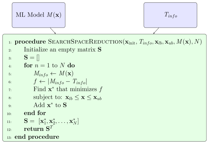
Figure 3: The search space reduction procedure requires a pre-trained ML model in order to generate the $\mathit{M}_{info}$ scalar value and compare it with the $\mathit{T}_{info}$ value. The objective of each of the $\mathit{N}$ optimization runs is to minimize the absolute difference between the two values. The $\mathit{N}$ value is predefined by the user and ultimately will determine the number of optimization solutions within the matrix $\mathbf{S}$ that will be used to form the reduced search space for the ML-enhanced inverse design framework.

The obtained solutions within the matrix $\mathbf{S}$ are then subjected to statistical processing and depends on the specific inverse design problem being solved (see Sect. 3 and Sect. 4), which yields the tighter lower and upper boundaries $\mathbf{lb}_{R}$ and $\mathbf{ub}_{R}$, respectively.

2.4 Machine Learning Model

The ML model $M$ takes as input the optimization design vector and maps it into $\mathit{M}_{info}$ which is further compared with the $\mathit{T}_{info}$ value, thereby minimizing the necessity for HF simulations.

The performance of three different ML algorithms is analyzed within this methodology – A Deep Neural Network (DNN), and two different gradient boosting algorithms – LightGBM (LGB) [27] and XGBoost (XGB) [8].

XGBoost or eXtreme Gradient Boosting (XGB) is a scalable tree boosting framework that effectively integrates a sparsity-aware algorithm alongside a weighted quantile sketch, thereby facilitating an approximate tree learning process. The combination of cache access patterns, elevated data compression, and sharding empowers XGBoost to construct an efficient and powerful tree boosting system.

LightGBM (LGB) is a robust and efficient gradient boosting framework aimed at enhanced performance and speed. It incorporates innovative strategies such as gradient-based one-side sampling and exclusive feature bundling to expedite processing and improve efficiency. LightGBM has a unique leaf-wise tree growth strategy, which deviates from the conventional level-wise approach seen in other boosting algorithms, and contributes to improved model accuracy by minimizing loss, thereby achieving faster convergence.

A DNN configured as an MLP is fundamentally composed of three distinct types of layers: the input, hidden, and output layers. These layers are constituted by artificial neuron nodes. The MLP model can incorporate multiple hidden layers as part of its neural architecture. Each neuron residing within the hidden and output layers utilizes a nonlinear activation function, echoing the complex processing mechanisms observed in the human brain [40]. This structure effectively facilitates the MLP’s ability to model and solve intricate nonlinear problems.

2.5 Metaheuristic Optimization Algorithms

Two distinct metaheuristic optimization algorithms will be compared: Particle Swarm Optimization (PSO) and Differential Evolution (DE). Both algorithms belong to the broader categories of swarm intelligence and evolutionary algorithms. Fundamentally, these categories rely on populations of agents that abide by specific rules to identify optimal solutions. Using both PSO and DE will demonstrate the general applicability of the ML-enhancement.

PSO is a population-based stochastic optimization algorithm, inspired by the social behavior of bird flocking or fish schooling [28]. In PSO, each individual particle in the swarm population represents a solution in the search space. Every particle updates its position based on its local best position, as well as the global best solution of the swarm. This cooperative search process, conducted through the iterative adjustment of velocities and positions increases the rate of convergence of the swarm towards the local or global optimum.

DE is a population-based stochastic search technique, commonly used for global optimization problems over continuous optimization design vectors [50]. In DE, the potential solutions are evolved over time via a simple arithmetic operation: a combination of mutation, crossover, and selection operations. Each individual in the population is a potential solution, and the evolution of these individuals is performed based on the differences between randomly sampled pairs of individuals within the population. The differential evolution of the population ensures a good rate of convergence, however, converging to a global optimum is not guaranteed. The success-history-based parameter adaptation (SHADE) variant of DE is used in this investigation. In the SHADE variant, the scaling factor and crossover rate are adaptively adjusted for each individual in the population based on a history of successful parameters. This dynamic adaptation allows for more effective exploration and exploitation of the search space, potentially improving the performance of the algorithm.

3 Airfoil Inverse Design

In this section, the airfoil inverse design problem is defined through the lens of the ML-enhanced optimization algorithm.

3.1 Airfoil Inverse Design Problem Description

The goal of the airfoil inverse design problem is to determine the optimal geometry of an airfoil given a set of target pressure coefficients on the surface of the airfoil. The parameters used for the airfoil inverse design and the search space reduction in the context of Eq. (3) and Eq. (4) are presented in Table 1. Each evaluation of the function $\varepsilon(\mathbf{x})$ (Eq. (3)) necessitates executing a flow simulation over a generated design.

Table 1: Mapping of problem-specific parameters for the airfoil inverse design to their corresponding general parameters used in the objective function and the search space reduction process.

General Parameter	Problem Specific Parameter
$\mathit{T}_{info}$	$C^{T}_{p_{min}}$
$\mathbf{T}$	$\mathbf{C}_{p}^{T}$
$\mathbf{P}^{C}(\textbf{x})$	$\mathbf{C}_{p}^{C}(\mathbf{x})$
$\mathit{M}_{info}$	$C_{p_{min}}$

$\mathbf{C}_{p}^{C}$$(\mathbf{x})$ denotes the computed pressure distribution around an airfoil based on the design vector $\mathbf{x}$, while $\mathbf{C}_{p}^{T}$ signifies the user-defined target pressure distribution measured at the same locations. $C^{T}_{p_{min}}$ denotes the target minimum pressure coefficient obtained from $\mathbf{C}_{p}^{T}$, and since the minimum pressure coefficient is used, the ML model’s task is to map optimization design vector $\mathbf{x}$ to the minimum pressure coefficient $C_{p_{min}}$ observed on the surface of the airfoil.

The airfoil inverse design optimization problem uses B-Spline approximation for the boundary definition, based on the $NACA0012$ airfoil, as this method offers superior shape parametrization [44]. Utilizing the splrep function from the scipy 1.9.1 module [53], the B-Splines are defined with coefficients, knots, a maximum degree of 5, and a smoothness parameter set at 0.00001. The knots generated by the splrep function as well as the degree and the smoothness of the splines remain unchanged throughout the optimization procedure.

The optimization design vector for the airfoil inverse design problem $\mathbf{x_{A}}$ is comprised of $N_{c}=30$ design variables with 15 lower ($\mathbf{c_{l}}$) and 15 upper ($\mathbf{c_{u}}$) airfoil surface B-Spline coefficients:

$$\mathbf{x_{A}}=[\mathbf{c_{l}},\mathbf{c_{u}}]^{T}\in\mathbb{R}^{N_{c}},\quad\begin{cases}\gamma\cdot\mathbf{c_{L0012}}\leq\mathbf{c_{l}}\leq\mathbf{0}\\ \mathbf{0}\leq\mathbf{c_{u}}\leq\gamma\cdot\mathbf{c_{U0012}}\\ \end{cases}$$ (6)

The bounds of these variables are determined by the $NACA0012$ lower and upper B-Spline coefficient vectors denoted as $\mathbf{c_{L0012}}$ and $\mathbf{c_{U0012}}$, respectively, scaled by a multiplication factor $\gamma=3$. The extracted lower boundary B-Spline coefficients in $\mathbf{c_{L0012}}$ are negative.

To prevent the possibility of overlap between the lower and upper coefficients in $\mathbf{c_{l}}$ and $\mathbf{c_{u}}$ (a scenario that may occur if certain coefficients converge to zero) a slight adjustment is made: 1e-5 is added to the $\mathbf{c_{u}}$ vector and subtracted from $\mathbf{c_{l}}$. This ensures that the box constraint in Eq. (3) remains intact. The constraints on $\mathbf{c_{l}}$ and $\mathbf{c_{u}}$ in Eq. (6) represent the prior lower and upper bounds ($\mathbf{x}_{lb}$ and $\mathbf{x}_{ub}$) for the ML-guided search space reduction process (Eq. (4)) as well as the boundaries used by the unenhanced optimization algorithms. The reconstructed lower and upper boundaries of the optimization design vector are shown in Fig. 4.

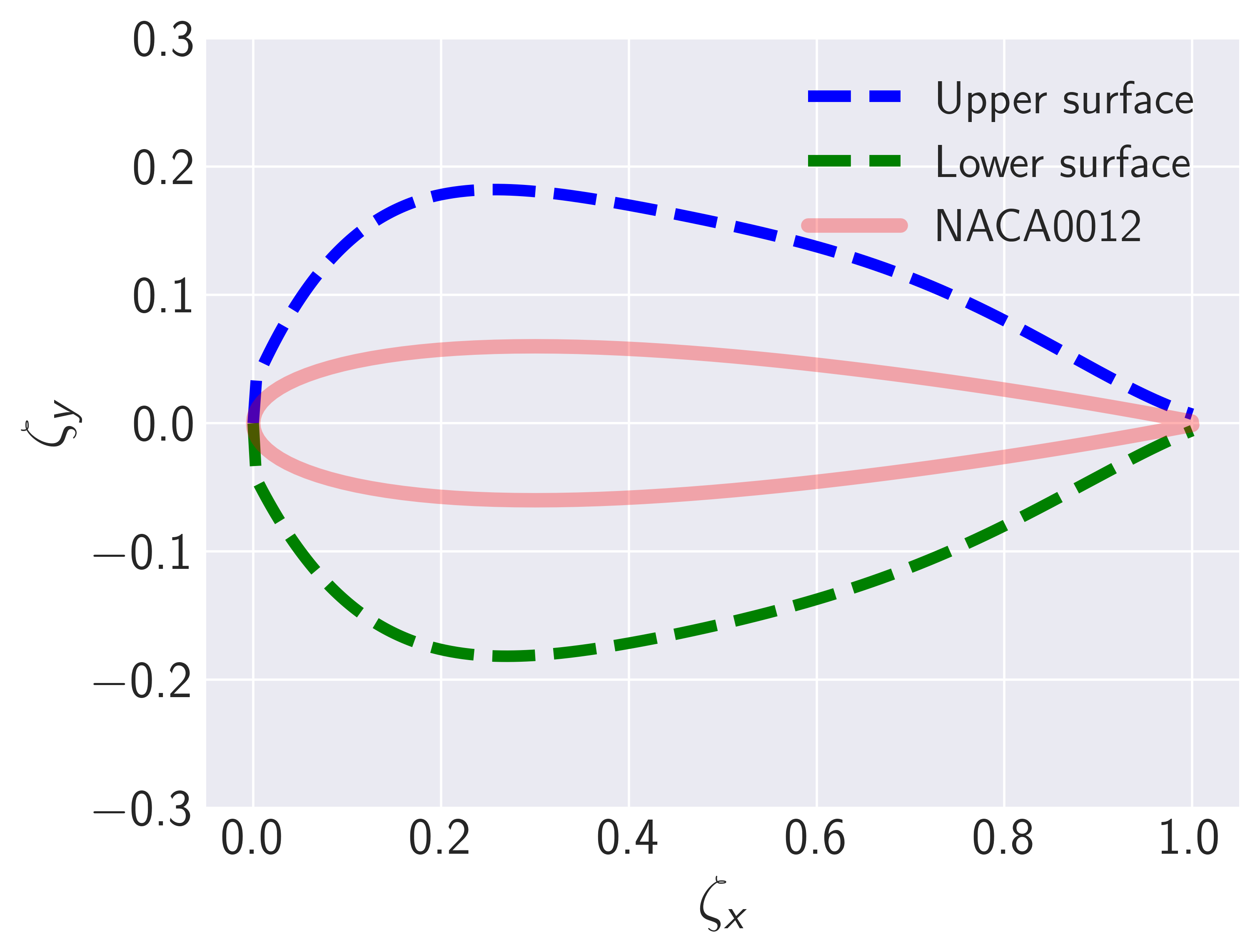
Figure 4: Optimization constraints generated by multiplying the $NACA0012$ baseline B-Spline coefficients by a factor of 3. The $\zeta_{x}$ and $\zeta_{y}$ axis are the chord-length normalized $x$ and $y$ coordinates.

3.2 Airfoil Inverse Design Search Space Reduction

The task of airfoil inverse design revolves around manufacturing processes where there exists a well-bounded optimal design. After the search space reduction technique is applied, a whole matrix of solutions $\mathbf{S}$ is obtained, as detailed in the Sect. 2.3. By statistically analyzing the matrix of optimal solutions derived from the ML model, the column-averaged values of the solution matrix $\mathbf{S}$ provide a meaningful representation of the probable design space. The matrix of solutions for the airfoil inverse design problem $\mathbf{S}_{A}$ is defined as

$$\mathbf{S}_{A}=\begin{bmatrix}\mathbf{x}^{opt}_{A_{1}}\\ \mathbf{x}^{opt}_{A_{2}}\\ \vdots\\ \mathbf{x}^{opt}_{A_{N}}\end{bmatrix}$$ (7)

Given the matrix $\mathbf{S}_{A}$ (where $\mathbf{x}^{opt}_{A_{N}}$ is the $N^{th}$ optimized solution of the airfoil inverse design problem), the element-wise mean value for each design vector dimension is defined as $\bar{\mathbf{x}}_{A}$. Furthermore, the averaged design vector $\bar{\mathbf{x}}_{A}$ is multiplied by a safety factor $\eta$ to ensure that the target design is within the new boundaries gives:

$$\mathbf{x_{A_{\eta}}}=\eta\cdot\bar{\mathbf{x}}_{A}$$ (8)

The design vector $\mathbf{x_{A_{\eta}}}$ represents an airfoil shape itself, i.e. it contains the design variables which are the lower and upper B-Spline coefficients, hence, new lower and upper boundaries ($\mathbf{lb}_{R}$ and $\mathbf{ub}_{R}$) are constructed based on this design vector for the airfoil inverse design problem. Different values of hyperparameter $\eta$ are investigated to assess their impact on the performance of the ML enhanced optimization, more specifically, $\eta\in\{1,1.1,1.2,1.3\}$. This approach is apt for the airfoil design as it reflects the realistic manufacturing constraints and ensures that the true design remains within these averaged values.

4 Scalar Field Reconstruction

In this section, the scalar field reconstruction problem is defined through the optimization design vector, constraints, and the search space reduction strategy.

4.1 Scalar Field Reconstruction Problem Description

The goal of the scalar field reconstruction problem is to determine the scalar boundary values based on a set of target scalar measurements on a given domain. The essence lies in optimizing the boundary conditions for a diffusion partial differential equation (PDE). This mathematical model describes how a scalar quantity spreads within a given domain. Instead of prescribing boundary conditions outright, the problem aims to find the ideal boundary conditions that, when applied to the diffusion PDE, result in a reconstructed scalar field that closely aligns with measured data. The diffusion PDE is defined as:

$$\frac{\partial s}{\partial t}=D\nabla^{2}s\quad\text{in }\Omega,\quad t\in[0,t_{max}]$$ (9)

where $s$ is the non-dimensional scalar value, $D$ is the diffusion coefficient set to 1 (m²/s), $t$ denotes the time (s), while $t_{max}$ denotes the maximum or end time of the simulation, and $\Omega$ is the domain. For the purposes of demonstrating the ML-enhanced inverse design framework, the $t_{max}$ is set to 0.1 s and is treated as a converged state, i.e. the scalar diffusion is treated as a quasi-transient problem.

The parameters used for the scalar field reconstruction and the search space reduction in the context of Eq. (3) and Eq. (4) are presented in Table 2.

Table 2: Mapping of problem-specific parameters for the scalar field reconstruction problem to their corresponding general parameters used in the objective function and the search space reduction process.

General Parameter	Problem Specific Parameter
$T_{info}$	$s^{T}_{{}_{max}}$
$\mathbf{T}$	$\mathbf{s}^{T}$
$\mathbf{P}^{C}(\textbf{x})$	$\mathbf{s}^{C}(\mathbf{x})$
$M_{info}$	${s_{max}}$

$\mathbf{s}^{C}$($\mathbf{x}$) denotes the computed scalar distribution on a given domain $\Omega$ based on the design vector $\mathbf{x}$ (denoted as $\mathbf{x_{s}}$ for the scalar field reconstruction problem) which is used to define the boundary condition, while $\mathbf{s}^{T}$ signifies the user-defined target scalar field measured at the same locations. $s^{T}_{{}_{max}}$ denotes the target maximum scalar value obtained from $\mathbf{s}^{T}$. The design vector constraint for the scalar field reconstruction problem is defined in Eq. (10). Since the maximum value of the $\mathbf{s}^{T}$ is used as the reduced-order information, the ML model maps the design vector $\mathbf{x_{s}}$ to the maximum scalar value ${s_{max}}$ observed in the domain.

$$\mathbf{x_{s}}=[s_{1},s_{2},\ldots,s_{I}]^{T}\in\mathbb{R}^{I},$$ (10)

$$\quad 0\leq s_{i}\leq s_{max}\quad\text{for}\quad i=1,2,\ldots,I.$$

The scalar design vector $\mathbf{x_{s}}$ consists of scalar values $s_{i}$ that collectively form a boundary condition for a given domain. The minimum scalar value at the boundary is defined as 0 and the maximum value $s_{max}$ is set to 30. For a HF simulation, the number of scalar values $i$ defined at the top of the domain $\Omega$ is 80 ($I=80$). However, with each evaluation of $\mathbf{x_{s}}$, it is necessary to obtain the $M_{info}$ value, and a discrepancy arises due to the ML model being trained with LF data where the number of scalar values was set to 20. In order to evaluate the $\mathbf{x_{s}}$ with $I=80$ using the ML model, the $\mathbf{x_{s}}$ are linearly interpolated and the scalar values at the LF boundary points are extracted in order to be evaluated by the ML model in order to predict $s{{}_{max}}$. In accordance with the diffusion PDE (Eq. (9)), the scalar boundary values are defined as the Dirichlet boundary condition (Eq. (11)) for the top part of the domain $\partial\Omega_{top}$:

$$s=g(\mathbf{x_{s}},t)\quad\text{on }\partial\Omega_{top},\quad t\in[0,T].$$ (11)

Other parts of the domain $\partial\Omega_{other}$ (left, right, bottom) are defined as the Neumann boundary condition:

$$\frac{\partial s}{\partial\mathbf{n}}=0\quad\text{on }\partial\Omega_{other},\quad t\in[0,T],$$ (12)

where $\mathbf{n}$ is the unit normal vector pointing outward from the domain. Finally, the mathematical domain $\Omega$ for the given scalar field reconstruction problem along with the appropriate boundary conditions are shown in Fig. 5.

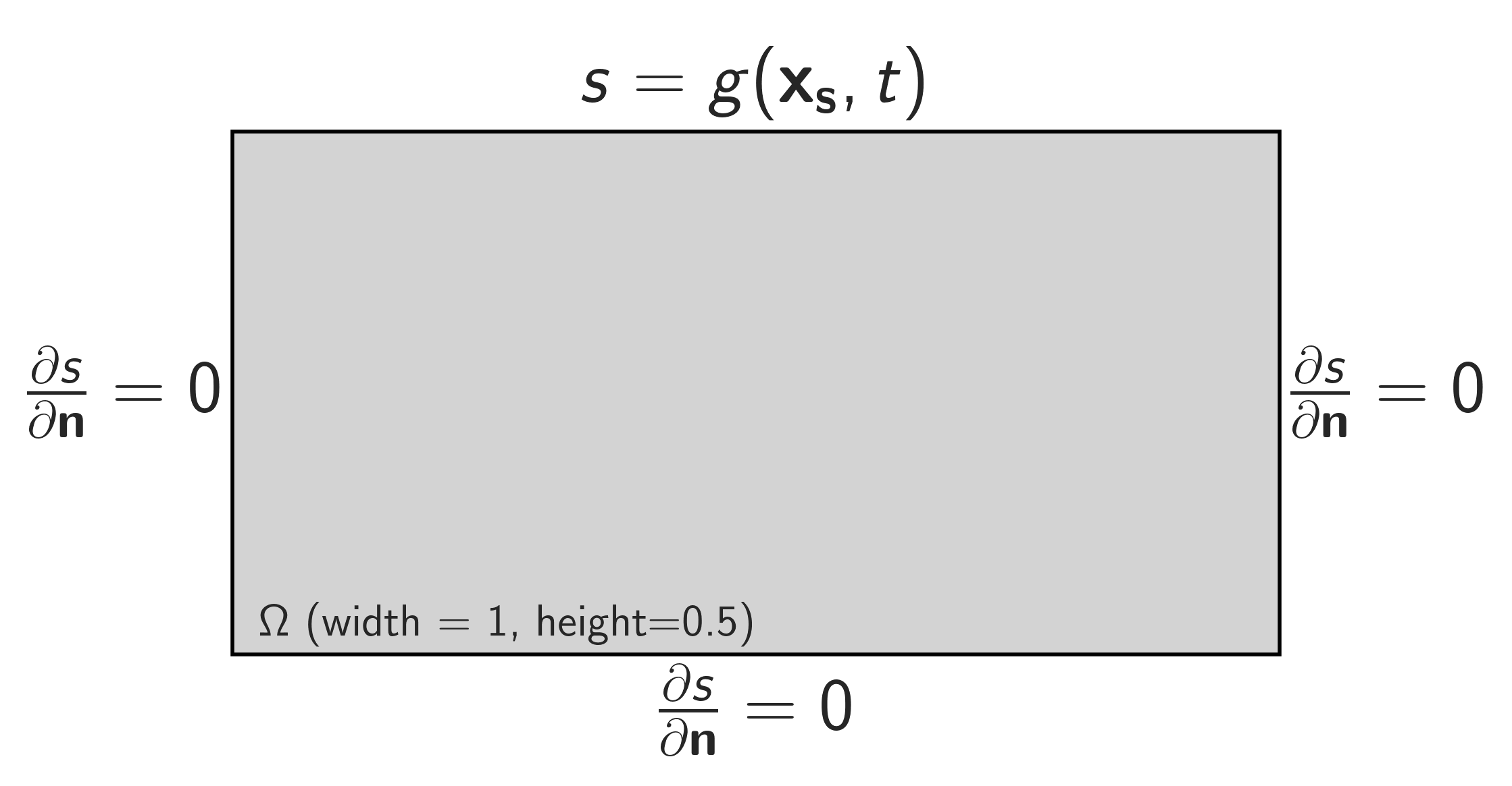
Figure 5: The mathematical domain $\Omega$ of the scalar reconstruction problem. The top boundary condition is the Dirichlet boundary condition where the optimization design vector $\mathbf{x_{s}}$ is set, while the bottom, left, and right parts are defined as the Neumann boundary condition. The height and width are presented in meters.

4.2 Scalar Field Reconstruction Search Space Reduction

In addressing the scalar field reconstruction problem, the size of the search space presents a significant challenge. This vast space comprises a myriad of valid solutions, making basic averaging methods inadequate for capturing its breadth. The solution matrix $\mathbf{S}_{s}$ of optimized design vectors $\mathbf{x_{s}}$ that contain boundary condition scalar values is defined as

$$\mathbf{S}_{s}=\begin{bmatrix}\mathbf{x}^{opt}_{s_{1}}\\ \mathbf{x}^{opt}_{s_{2}}\\ \vdots\\ \mathbf{x}^{opt}_{s_{N}}\end{bmatrix}$$ (13)

where $\mathbf{x}^{opt}_{s_{N}}$ is the $N^{th}$ optimized design vector. Subsequently, the design vectors within matrix $\mathbf{S}_{s}$ are subjected to regression model fitting. This fitting utilizes polynomials of degree $d$ $\in\{1,2,3,4\}$ for each $n=1,2,\ldots,N$ design vector, forming the new regression model solution matrix $\mathbf{S}_{sreg}$ as:

$$\mathbf{S}_{sreg}=\bigcup_{n=1}^{N}\bigcup_{d=1}^{4}\text{RegressionFit}(\mathbf{x}^{opt}_{s_{n}},\text{degree}=d)$$ (14)

Polynomial regression coefficients are determined using the numpy 1.24.3 function polyfit for 20 equally spaced points between 0 and 1 (which corresponds to the LF discretization), and this regression model, generated by the function poly1d, is subsequently evaluated for the HF discretization ($I=80$) with equally spaced points between 0 and 1, resulting in the final $\mathbf{S}_{sreg}$ set. To determine the new optimization boundaries for the scalar field reconstruction problem, the maximum scalar value is extracted from the flattened matrix $\mathbf{S}_{sreg}$ set: $max(\mathbf{S}_{sreg})$ defines the upper optimization boundary value for each dimension $I$, thus forming the new upper boundary $\mathbf{ub}_{R}$. For safety reasons, the lower boundary $\mathbf{lb}_{R}$ remains as specified in Eq. (10), i.e., $\mathbf{0}$.

Fig. 6 illustrates an instance of the search space reduction process. The green line represents the true solution, the blue line shows the reduction of the search space (approximately 50% pruned) as described above and the black line represents the average of $N$ optimized boundary conditions for comparison. The green curve lies below the black curve, suggesting that the space reduction methodology used for the airfoil inverse design problem might be similarly effective here.

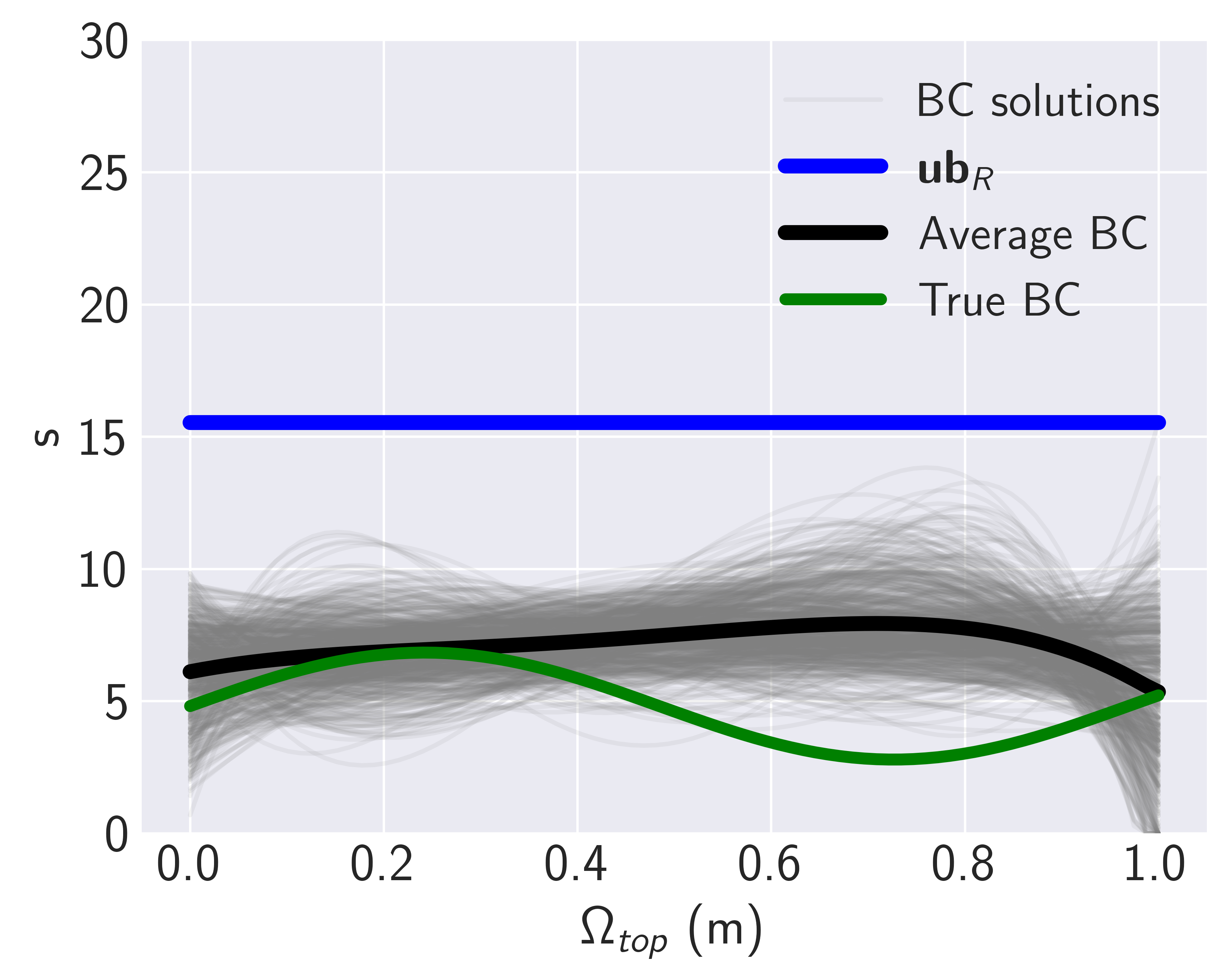
Figure 6: Scalar field reconstruction search space reduction example. The grey lines are the $N$ solutions within the matrix $\mathbf{S}_{s}$, the black line is the average value of the solutions in matrix $\mathbf{S}_{s}$, the green line is the true boundary condition that corresponds to the $\mathbf{T}$ field measurements, and the blue line is the new upper boundary $\mathbf{ub}_{R}$ obtained with the search space reduction procedure described in this section.

5 Numerical Experiments Setup and Hyperparameters

In this section, the airfoil inverse design instances and the boundary conditions for the scalar reconstruction problems are described. Details concerning the solvers utilized for simulating these inverse design problems are provided. Additionally, the section offers insights into the ML dataset generation, hyperparameters of optimization and machine learning algorithms, and the metrics applied to gauge the accuracy of the ML models.

5.1 Airfoils and Aerodynamic Flow Analysis

The airfoils $RAE2822$ and $NACA2410$ are used for the numerical analysis. They both exhibit asymmetry along the chord line unlike the base $NACA0012$ airfoil which was used to construct the original lower and upper boundaries of the decision vector. The $NACA2410$ airfoil is a member of the same family as the $NACA0012$, which serves as a reference for defining the B-Spline coefficient constraints. The $RAE2822$ airfoil is one of the most widely used benchmark airfoils in the field of aerodynamic shape optimization and inverse design [32, 10, 18, 33]. The shapes of both airfoils are shown in Fig. 7.

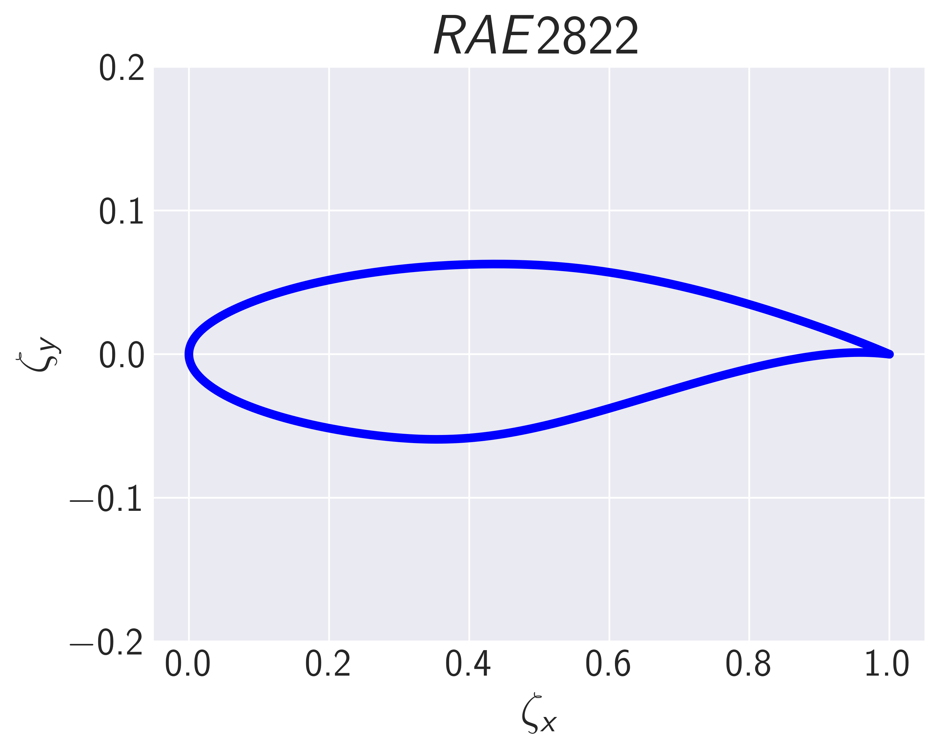
(a)

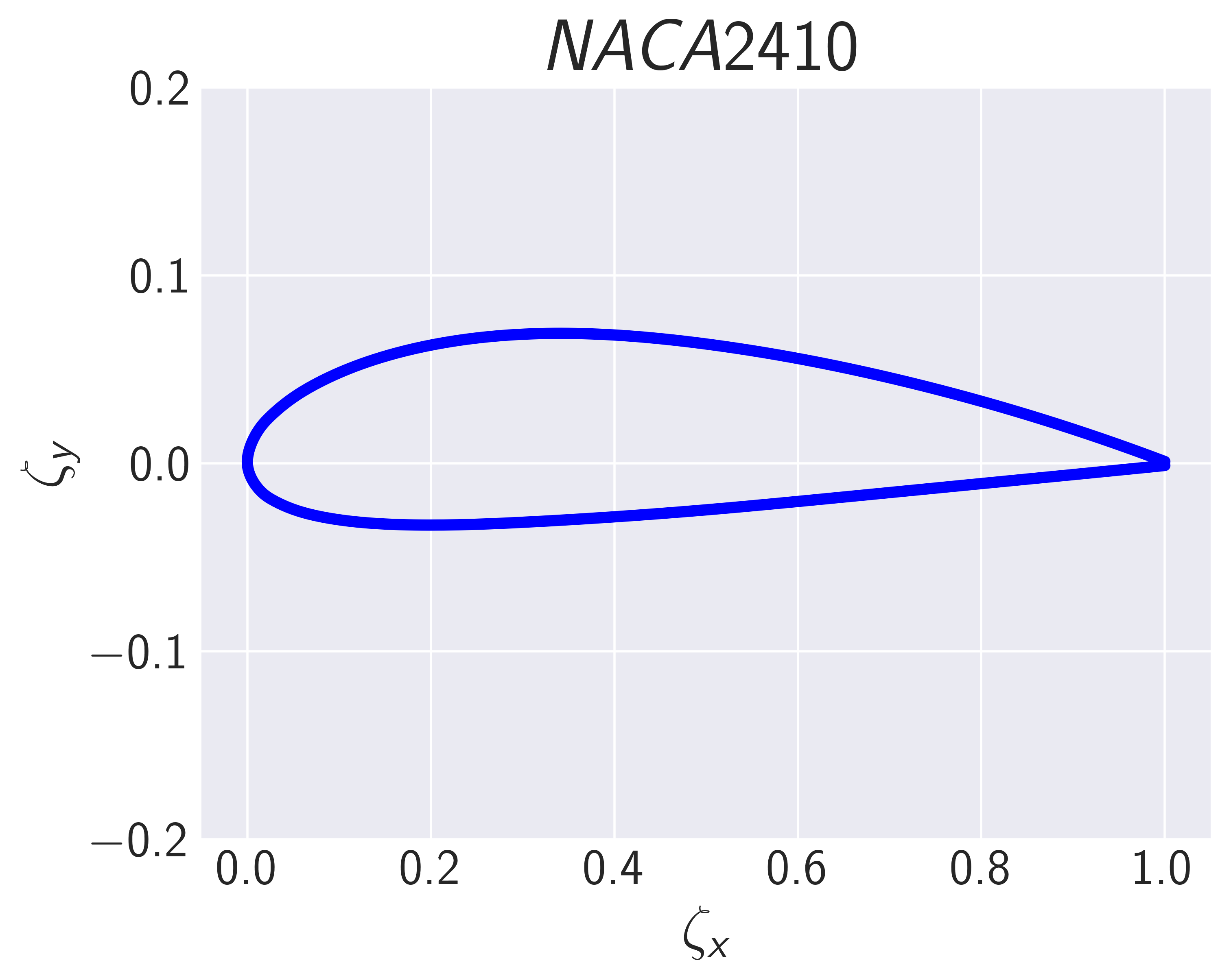
(b)

Figure 7: Investigated airfoil geometries: (a) $RAE2822$ airfoil (b) $NACA2410$ airfoil. Due to the optimization constraints being generated based on the $NACA0012$ airfoil as well as the ML model dataset (Sect. 5.3), the $RAE2822$ shape provides a harder optimization challenge due to its larger deviation from the camber line.

For both investigated airfoils, the flow simulation parameters–Reynolds number (Re), Angle of Attack (AoA), and Mach number (Ma)–were set to 5$\cdot 10^{7}$, 4, and 0, respectively. The target pressure coefficients were derived from these flow conditions and the specific airfoils, including the $C^{T}_{p_{min}}$ values. Specifically, for the $RAE2822$, $C^{T}_{p_{min}}=-2.27$ and for the $NACA2410$, $C^{T}_{p_{min}}=-1.58$. The aerodynamic flow analysis was conducted using XFOIL. This software package, specifically designed for subsonic airfoil analysis, served as the primary tool for assessing the pressure coefficients around the airfoil [11]. The Python wrapper for XFOIL simulations – xfoil 1.1.1 [54] was utilized.

XFOIL operates on a numerical panel method, which is integrated with a boundary layer model, facilitating accurate predictions of flow behavior around an airfoil. Through an iterative process, XFOIL effectively solves the potential flow equation for inviscid flows and the integral boundary layer equations for momentum and energy in viscous flows. It is optimally designed to accommodate incompressible flow scenarios with a Reynolds number between $10^{6}$ and $10^{8}$. The number of discretization panels used for XFOIL simulations determines the fidelity of the simulation. It has been shown by Morgado et al [39] that XFOIL is more accurate than other methods for high lift low Reynolds number airfoils. In HF simulations, the discretization panel value is set to 300, while in LF simulations it is reduced to 100.

For each analysis, XFOIL takes as input the airfoil design, which is represented by the coordinates generated by the optimization variables: B-Spline degree, coefficients, and knots. Additional parameters, such as Re, AoA, and Ma must be specified for each simulation. Each XFOIL evaluation outputs the pressure coefficients measured around the airfoil which are compared with the target pressure coefficients. The number of iterations was set to 400 for every simulation, while the panel bunching parameter was set to 1, the trailing and leading edge density ratio was set to 0.15, and the refined-area-leading edge panel density ratio was set to 0.2.

While the proposed inverse design framework can leverage various computational fluid dynamics (CFD) analysis tools, XFOIL has been selected for its computational efficiency and as a proof-of-concept. In the future, this methodology can easily be expanded to incorporate more sophisticated approaches, such as Large Eddy Simulation (LES), which has significantly higher computational demands.

5.2 Scalar Diffusion Boundary Conditions and Solver

Two distinct boundary conditions (BC) were investigated to demonstrate the versatility of a single ML model across various scenarios. As depicted in Fig. 8, one BC exhibits a sinusoidal pattern, whereas the other adheres to a linear trend. Both BCs were used to generate $\mathbf{s}^{T}$ arrays. The values were measured at locations given in Appendix A (Fig. 20 and Table 9). The $T_{info}$ ($s_{max}$) value for the sinusoidal BC (Fig. 8(a)) was 5.67, while for the linear BC (Fig. 8(b)) it was 9.1.

To simulate the BCs over the domain, the open source computational fluid dynamics library OpenFOAM 9 was used [25]. More specifically, the laplacianFoam diffusion PDE solver was used. The details about the LF and HF domains are presented in Table 3. The LF scalar diffusion simulation is solved for a computational domain that is 16 times smaller than the HF computational domain.

(a)

(b)

Figure 8: Two investigated boundary condition cases: (a) Sinusoidal boundary condition (b) Linear boundary condition. The x-axis defines the top boundary domain which ranges from 0 to 1, while the y-axis is the scalar value for each $\Omega_{top}$.

Table 3: “Total cells” refers to the number of cells within the computational domain. “Top BC cells” signifies the quantity of cells along the $\Omega_{x}$-axis direction, where the Dirichlet boundary condition is applied. $\delta\Omega_{x}$ and $\delta\Omega_{y}$ represent the cell sizes in the $\Omega_{x}$ and $\Omega_{y}$ axis directions, respectively.

Type	Total cells	Top BC cells	$\delta\Omega_{x}$	$\delta\Omega_{y}$
LF	400	20	0.05	0.025
HF	6400	80	0.0125	0.00625

5.3 ML model training datasets

In this section, the ML dataset procedure is presented for both the airfoil inverse design problem and the scalar field reconstruction.

5.3.1 Minimum Pressure Coefficient Dataset

In order to train the ML model, a suitable dataset must be generated. As defined in Sect. 3, the $M_{info}$ value corresponds to the minimum pressure coefficient, denoted $C_{p_{\text{min}}}$, necessitating the simulation of aerodynamic properties across a wide array of geometries and their mapping to respective $C_{p_{min}}$ values. This dataset was assembled utilizing the Latin Hypercube Sampling (LHS) design of experiment technique. Input features for training the ML model were generated using LHS as B-Spline coefficients ($\mathbf{c_{u}}$ and $\mathbf{c_{l}}$ in Eq. (6)). Each B-spline coefficient was subsequently transformed into an airfoil geometry to obtain the corresponding $C_{p_{min}}$ value. All data were generated utilizing LF simulations, employing 100 discretization panels, with the flow parameters defined in Sect. 5.1. A total of 15000 LF simulations were conducted, meaning a total of 15000 B-Spline and C${}_{p_{min}}$ pairs were generated.

5.3.2 Maximum Scalar Dataset

The $M_{info}$ for the scalar field reconstruction requires identification of the maximum scalar value, $s_{max}$ within the domain. To curate a dataset, variations were made in the BC scalar values. For every distinct scalar value set, a simulation was executed, capturing the corresponding $s_{max}$ value. An in-depth analysis of the methodology employed to generate diverse BCs for this reconstruction problem can be found in Fig. 21. For dataset creation, 15000 LF simulations were executed using OpenFOAM 9, with full details provided in Sect. 5.2.

5.4 ML Model Accuracy Metrics

The accuracy of all ML models was assessed using the $RMSE$ (Eq. (15)) since it is used to evaluate the $\omega$ value within the ML-enhanced framework (as shown in Fig. 2).

$$\text{$RMSE$}=\sqrt{\frac{\sum_{l=1}^{L}(y_{l}-\hat{y}_{l})^{2}}{L}}$$ (15)

The variables $y_{l}$, $\hat{y}_{l}$, and $L$ represent the $l^{th}$ actual value, the $l^{th}$ ML model prediction, and the test set size, respectively. The K-Fold cross-validation procedure ($k=5$) was used to evaluate the accuracy and uncertainty of all three investigated algorithms.

5.5 PSO and DE Optimization Algorithm Hyperparameters

For the two examined problems, the swarm size and the population size parameters for the PSO and DE algorithms were both set to 10. Both DE and PSO implementations Indago 0.4.5 [23] Python module for numerical optimization were used.

For the PSO algorithm, the inertia parameter was set at 0.8. The cognitive and social rates of the swarm were standardized to 1, mainly based on the default recommendations with the Python module.

For DE, the key hyperparameters, such as the archive size factor, historical memory size, and mutation rate, were configured to 2.6, 4, and 0.11, respectively, following recommendations from the utilized Python module.

5.6 ML Algorithms Hyperparameters

In this subsection, the optimized hyperparameters of all investigated ML algorithms are presented. The best performing algorithm was further used as a part of the enhanced inverse design framework. All three ML algorithms were optimized using the Python framework for hyperparameter optimization Optuna 3.1.0. [2]. The number of trials for all three algorithms was 100, and Optuna-based hyperparameter optimization goal was to minimize the average $RMSE$ of a shuffled K-Fold ($k=3$) cross-validation procedure. The ML algorithms were separately tuned for both investigated problems/datasets (described in Sect. 5.3), and 15000 LF data instances were used for optimization. The optimal set of hyperparameters was independently selected for each of the three investigated algorithms, based on the results from 100 trials conducted using Optuna.

The XGB algorithm hyperparameters used are presented in Table 4. The max_depth parameter controls the depth of each tree, the n_estimators defines the total number of gradient boosted trees in the model, learning_rate scales the contribution of each tree when it is added to the ensemble of trees, colsample_bytree and subsample parameters specify the fraction of the randomly sampled features and data instances used to construct each tree, respectively, and gamma, reg_alpha and reg_lambda are regularization parameters. The Python module xgboost 1.7.4 was used.

Table 4: XGB model hyperparameters tuned with the Optuna Python framework. The best solution of 100 trials is shown. The first column denotes the names of the tuned hyperparameters, while the second column shows the values obtained for the airfoil inverse design (AID) problem, and the third column shows the parameter values for the scalar field reconstruction (SFR) problem.

Hyperparameter	AID	SFR
max_depth	4	5
n_estimators	500	500
learning_rate	0.07	0.06
colsample_bytree	0.94	0.19
subsample	0.54	0.36
gamma	0.42	1.33
reg_alpha	2.44	0.51
reg_lambda	4.16	0.20

The LGB model hyperparameters are presented in Table 5. The num_iterations parameter controls the number of boosting iterations performed. Each iteration builds a new tree that boosts the performance of the model. The learning_rate scales the contribution of each tree when it is added to the model (similarly as XGB), lambda_l1 and lambda_l2 are L1 and L2 regularization parameters added in order to reduce overfitting. The parameter num_leaves controls the complexity of the model, and min_child_samples refers to the minimum number of data instances a leaf node must have after a split, as a form of regularization. The feature_fraction parameter defines tha fraction of features used at each training iteration, while bagging_fraction determines the number of data instances used at each iteration. Both parameters are also used as a form of regularization. The Python module LightGBM 3.3.5 was used.

Table 5: LGB model hyperparameters tuned with the Optuna Python framework (the best solution out of 100 for each problem). The first column denotes the names of the tuned hyperparameters, the second column shows the values obtained for the airfoil inverse design (AID) problem, and the third column shows the parameter values for the scalar field reconstruction (SFR) problem.

Hyperparameter	AID	SFR
num_iterations	2500	2500
learning_rate	0.0187	0.0190
lambda_l1	1.78	0.40
lambda_l2	7.43	6.71
num_leaves	41	68
min_child_samples	37	99
feature_fraction	0.77	0.56
bagging_fraction	0.45	0.52

The hyperparameters for the MLP are detailed in Table 6. The LeakyReLU activation function was applied to all hidden layers in the AID problem, whereas the SFR used ReLU. Monte Carlo dropout layers were integrated into the architecture to reduce overfitting. During training for both problems, 30% of the data was reserved for validation. An early stopping criterion with a patience value of 20 was set based on the validation loss to further combat overfitting. The MLP was implemented in Tensorflow 2.11.0 [1].

Table 6: MLP hyperparameters tuned with the Optuna Python framework (the best solution out of 100 trials is shown for each problem). The first column denotes the names of the tuned hyperparameters, the second column shows the values obtained for the airfoil inverse design (AID) problem, and the third column shows the parameter values for the scalar field reconstruction (SFR) problem.

Hyperparameter	AID	SFR
Layers	3	2
Neurons per layer	92,116,34	388,322
Dropout per layer	0.1,0.1,0.0	0.1,0.0
Activation function	LeakyReLU	ReLU
Optimizer	Adam	Adam
Epochs	100	500
Batch size	128	64
Learning rate	0.00083	0.00060

6 Results and Discussion

In this section, the results and analyses for the ML model, search space reduction, and ML-enhanced framework for both demonstration problems are detailed. An in-depth hyperparameter analysis of the ML-enhanced framework is showcased, followed by overarching recommendations for optimal utilization. The section concludes by highlighting the advantages and limitations of the proposed technique.

6.1 Machine Learning Models Results

In this subsection, the ML model results for both the AID and SFR problems are presented through the accuracy metrics presented in Sect. 5.4.

6.1.1 AID ML Model Results

Fig. 9 presents the $RMSE$ scores for the three ML algorithms applied to the AID problem for varying dataset sizes. The dataset size was varied in order to assess the influence it has on the ML-enhanced framework, and to obtain the learning curve for each algorithm. All models show that the larger the dataset size, the better (lower) the resulting $RMSE$. It can be seen that for smaller datasets, XGB has better performance than LGB and MLP, but its accuracy marginally lags when leveraging all 15000 data instances for training and cross-validation. Given its overall top performance, XGB (trained with four different dataset sizes) was selected as the ML model for the inverse design framework, and the K-fold cross-validation $RMSE$ values used for further analysis are presented in Table 7.

Figure 9: The mean (solid lines) and standard deviation (shaded areas) K-Fold $RMSE$ for the three investigated ML algorithms for the AID problem. Lower $RMSE$ values are better.

Table 7: XGB $RMSE$ values used for calculating the $\omega$ threshold parameter for each scenario and dataset size.

Dataset size	$RMSE$
500	0.81
1000	0.61
5000	0.39
15000	0.34

6.1.2 SFR ML Model Results

Fig. 10 shows the $RMSE$ values of the three ML algorithms when applied to the SFR problem using different dataset sizes. The results show the MLP’s superior performance over both LGB and XGB across all dataset sizes. As a result, the MLP was selected as the ML model within the inverse design framework for the SFR problem. The specific K-fold cross-validation $RMSE$ values for the MLP, which were used to compute the $\omega$ parameter for the SFR problem, are detailed in Table 8. Given the minimal performance difference between the models trained with 5000 and 15000 instances, only three distinct models trained on three different amounts of data were compared within the ML-enhanced framework.

Figure 10: The mean (solid lines) and standard deviation (shaded areas) K-Fold $RMSE$ for the three investigated ML algorithms for the SFR problem.

Table 8: MLP $RMSE$ values used for calculating the $\omega$ threshold parameter for each of the two SFR BC scenarios and dataset size.

Dataset size	$RMSE$
500	7.63
1000	4.27
5000	0.78

6.2 Search Space reduction with the ML Model

In this subsection, the results of the search space reduction technique for both investigated problems are presented. To generate the new boundaries $\mathbf{lb}_{R}$ and $\mathbf{ub}_{R}$ of the reduced search space, models trained on different dataset sizes were compared. The DE was employed to solve Eq. (4) 150 times ($N=150$ solutions). The DE algorithm was configured with a maximum of 800 function evaluations, and the population size was set to equal the dimensionality of the optimization vector i.e. 20 for SFR and 30 for AID. A comparative analysis of different $N$ values is provided in Appendix C.

6.2.1 AID Search Space Reduction

In Sect. 6.1, the choice of the XGB algorithm was justified by its marginal superiority over other algorithms, especially when various training data sizes are taken into account. For the purpose of generating a reduced search space, the XGB was trained using data instances of sizes 500, 1000, 5000, and 15000. The results of the edge cases of the XGB-produced boundaries $\mathbf{lb}_{R}$ and $\mathbf{ub}_{R}$ are illustrated in Fig. 11. Since every solution in the matrix $\mathbf{S}_{A}$ represents an airfoil itself with lower and upper shape coefficients, the new lower and upper boundaries were derived solely by averaging the solution matrix $\mathbf{S}_{A}$ where $\eta=1$ encompass the genuine target designs. A notable overlap is observed in a section of the upper trailing edge between the target and the new boundary ($\zeta_{x}>0.8$). When the safety factor is increased to its maximum investigated value of $\eta=1.3$, this overlap at $\zeta_{x}>0.8$ significantly diminishes, and a noticeable distinction is achieved between the new and the original boundaries (Figures 11(b) and 11(d)).

When training the XGB model with different numbers of instances, only minor variations in results emerge. This suggests that the ML model trained with a small dataset suffices to prune a segment of the design space for such problems. This observation holds for both $NACA2410$ and $RAE2822$ search space reductions, as illustrated in Fig. 11. Finally, an analysis of how the number of solutions $N$ effects the change in the airfoil shape and the search space reduction is shown in Fig. 22 (Appendix C).

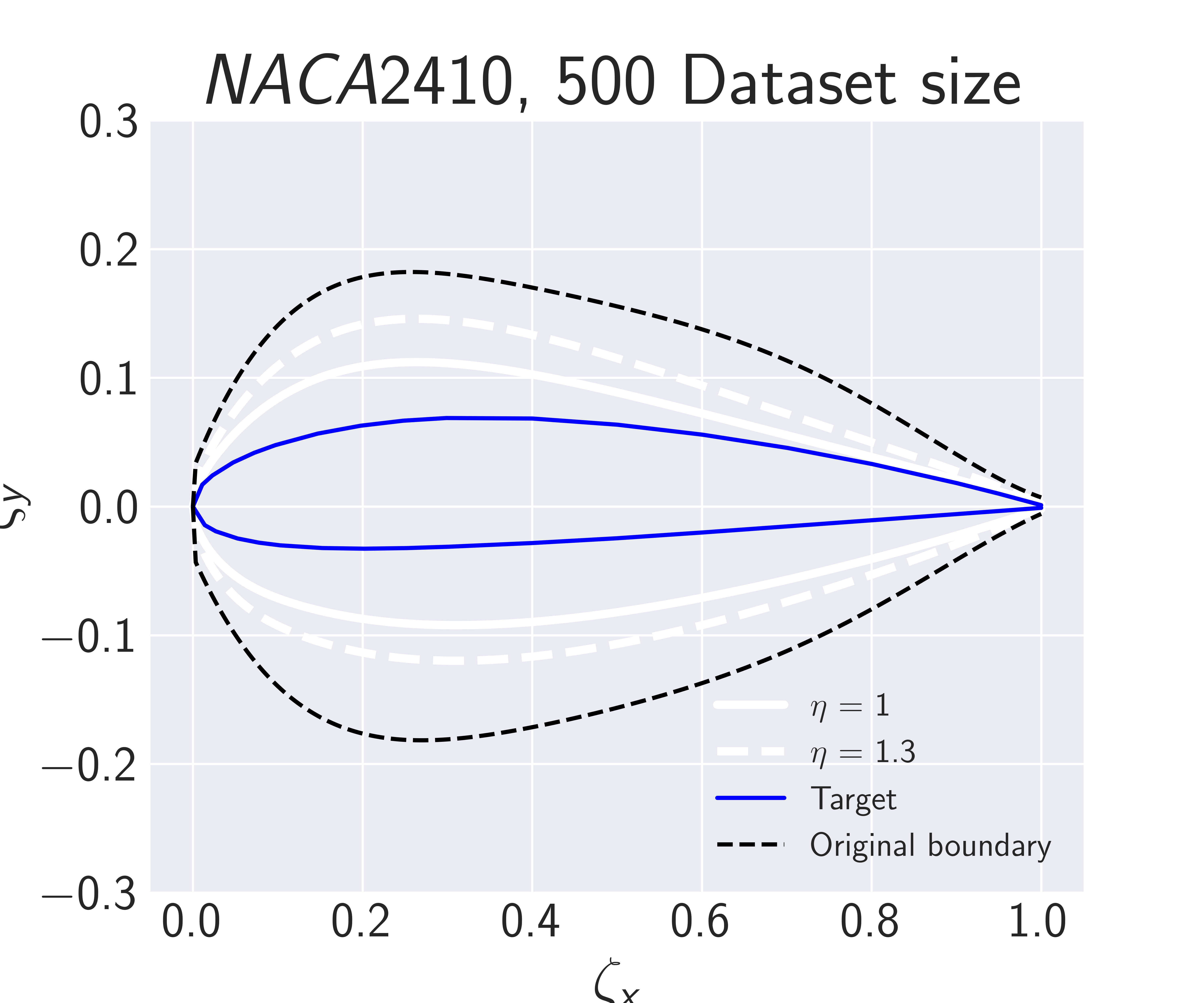
(a)

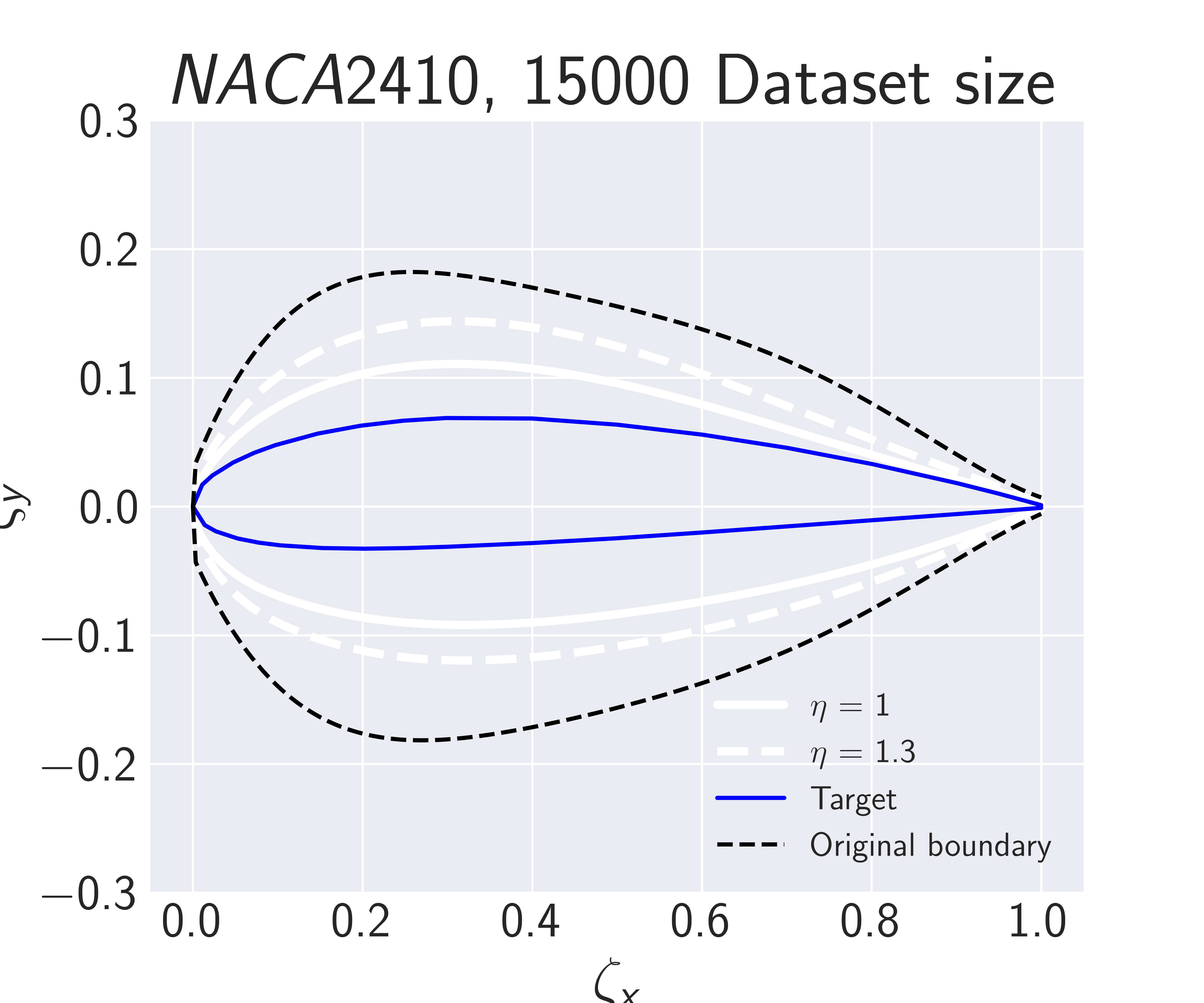
(b)

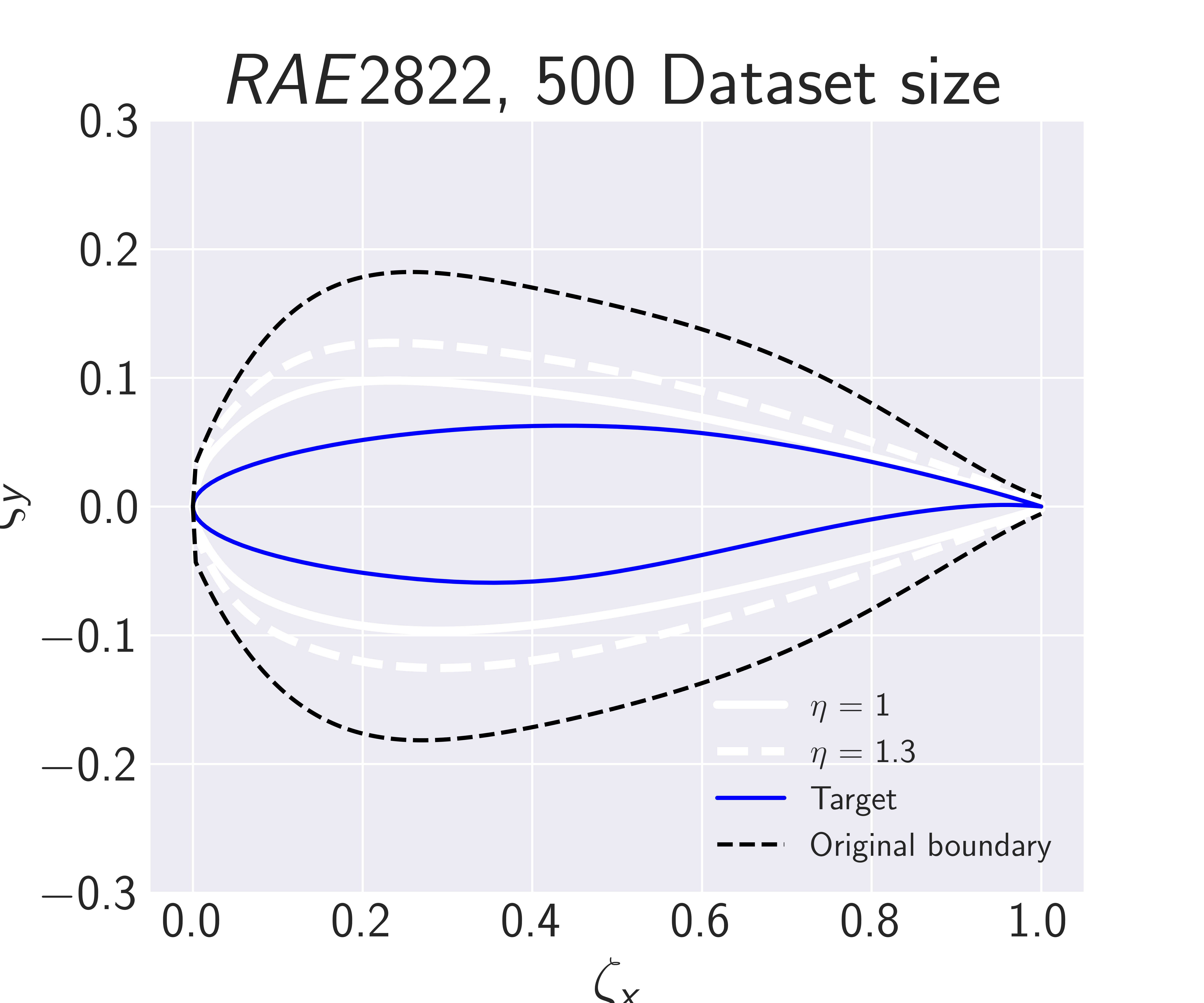
(c)

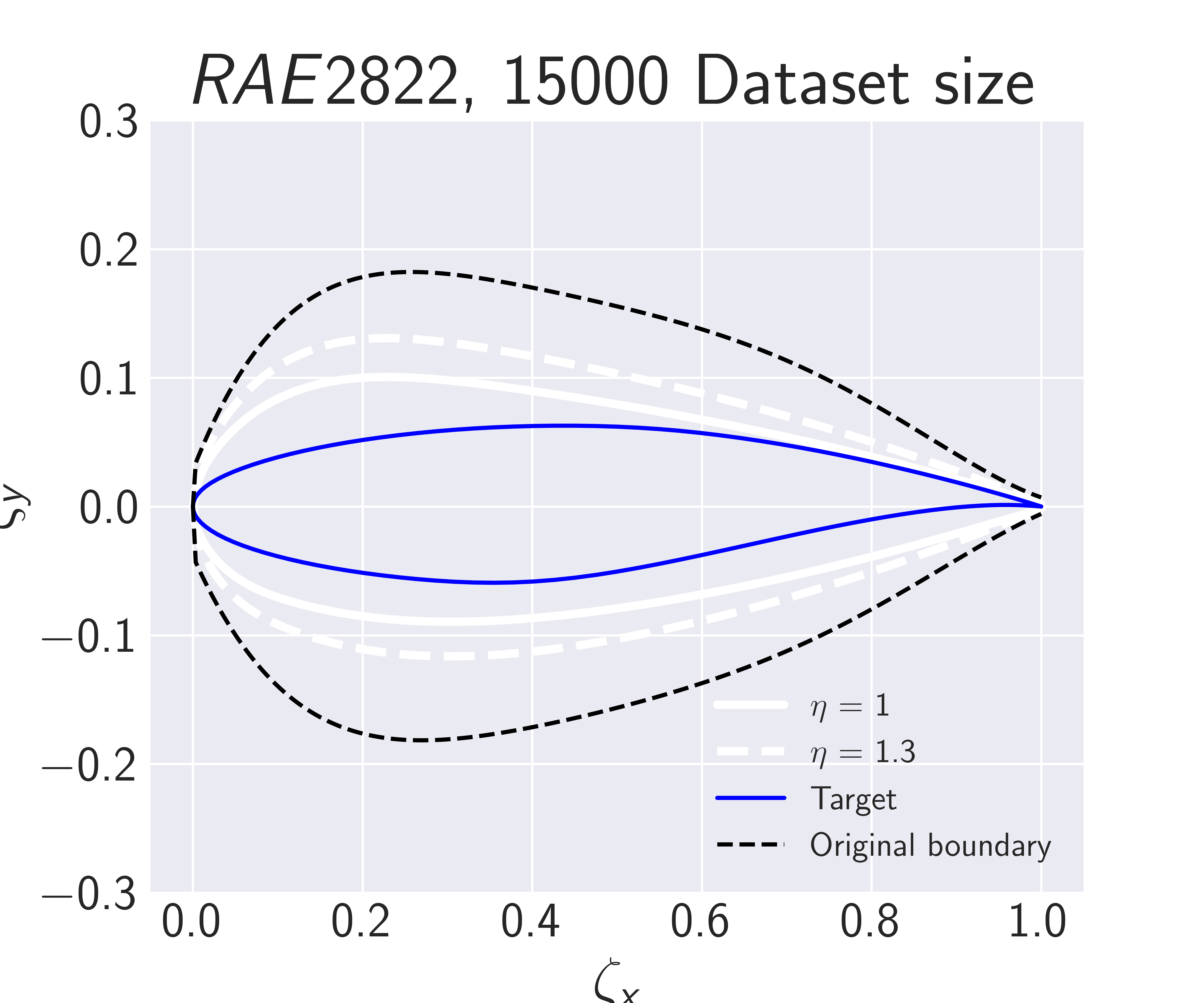
(d)

Figure 11: Search space reduction technique results generated by the XGB model: (a) $NACA2410$ with dataset size 500 (b) $NACA2410$ with dataset size 15000 (c) $RAE2822$ with dataset size 500 (d) $RAE2822$ with dataset size 15000. The white lines indicate the reduced search space boundaries, i.e. $\mathbf{lb}_{R}$ and $\mathbf{ub}_{R}$ for different values of $\eta$. There is no noticeable difference between the white lines when the dataset size is increased, indicating that a significant search space reduction is achievable even with an ML model trained on a small dataset.

6.2.2 SFR Search Space Reduction

For the SFR problem, the MLP outperformed the other investigated algorithms in modeling $s_{max}$. Fig. 12 displays the MLP results of the search space reduction. The MLP was trained with dataset sizes 500, 1000, and 5000. Across both BC scenarios, all three MLP models significantly reduce the size of the search space, confining the $\mathbf{ub}_{R}$ value between $s=13$ and $s=18$ (43% to 60% of the design space pruned). Compared to the airfoil problem, these newly produced boundaries exhibit greater sensitivity to changes in dataset size, but all three can be reliably incorporated into the ML-enhanced inverse design framework without losing the true solutions. Additionally, Fig. 23 (Appendix C) presents an analysis of how the number of solutions, $N$, impacts both cases of the SFR problem.

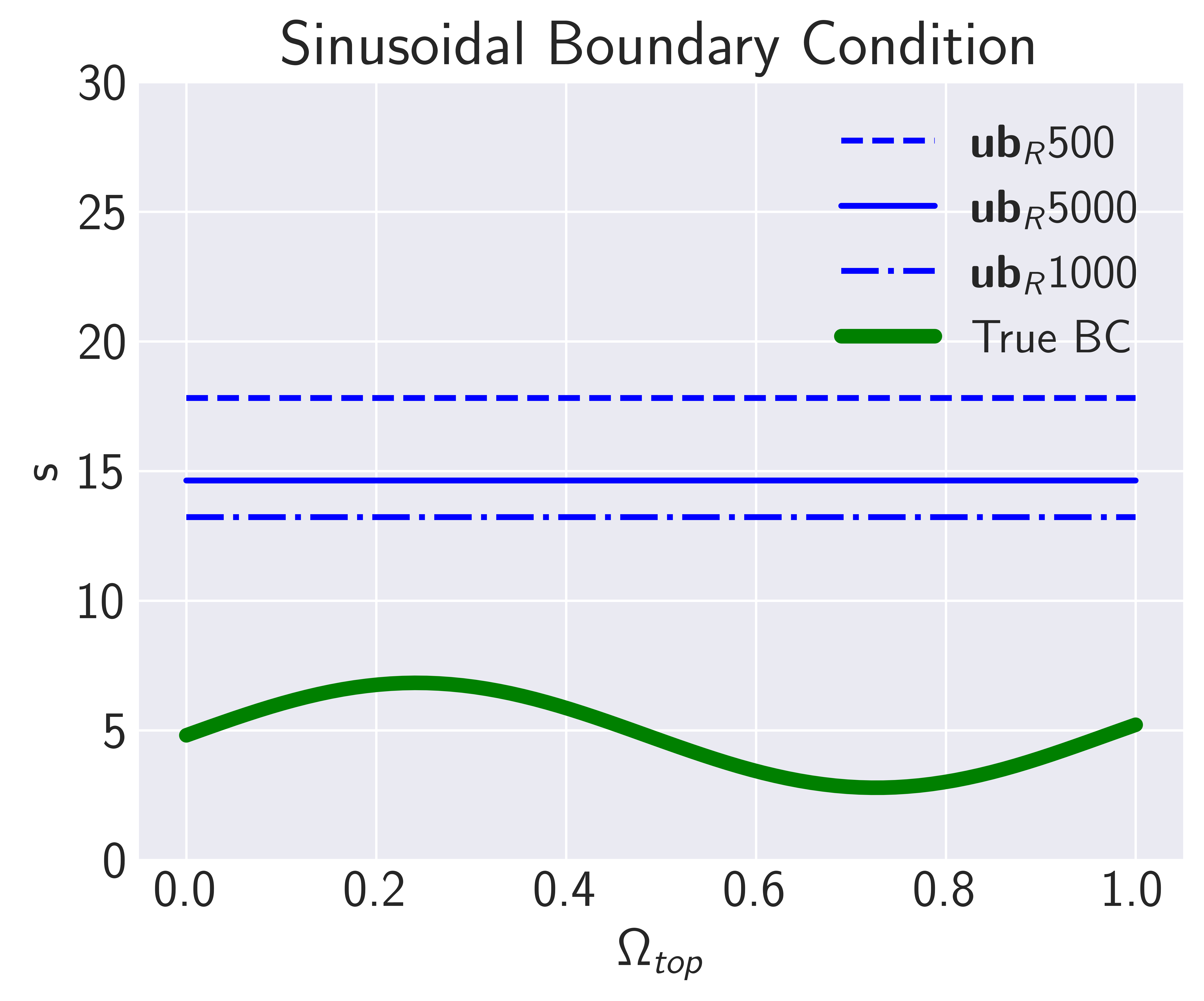
(a)

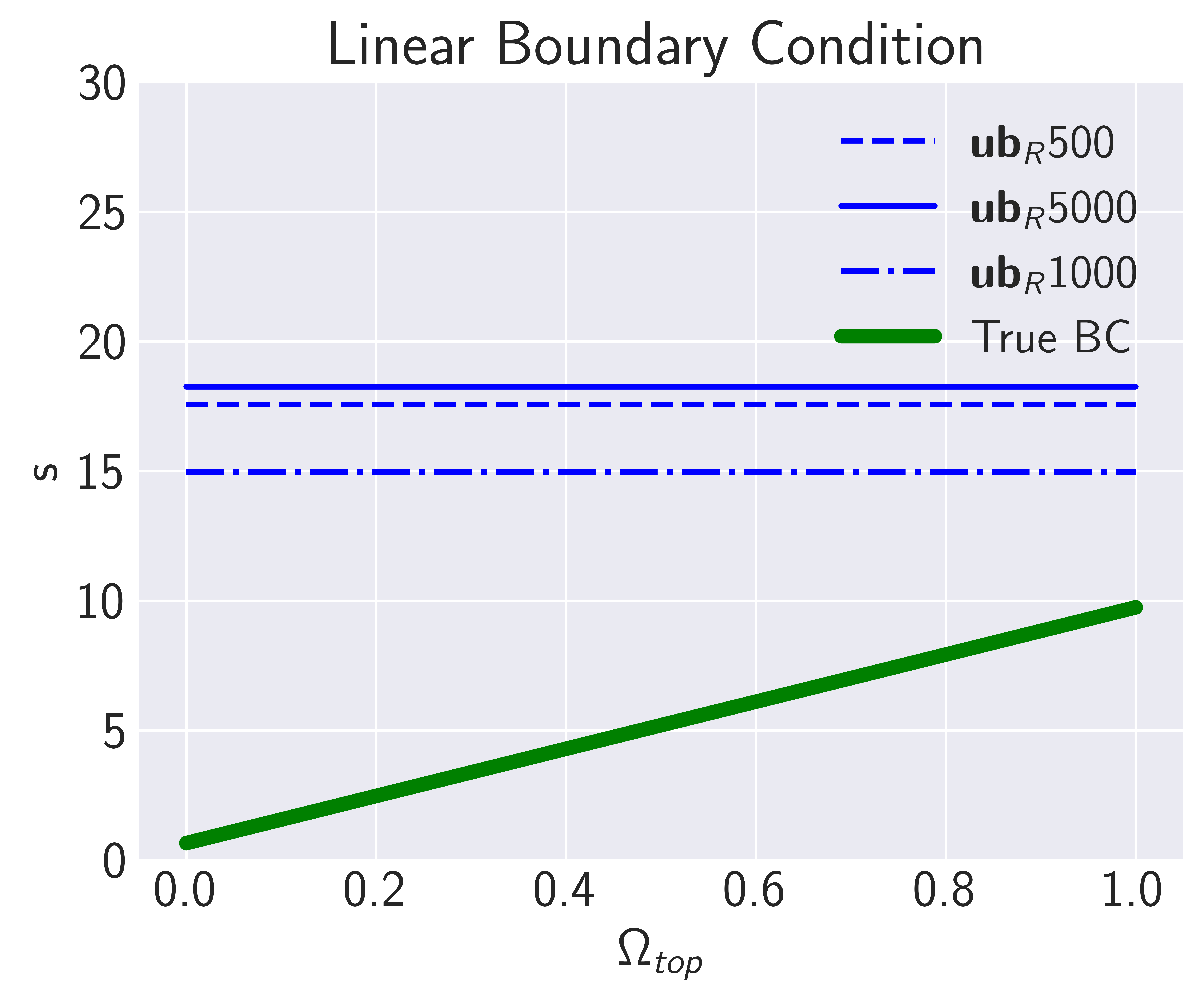
(b)

Figure 12: The search space reduction technique developed for the SFR problem implemented on two distinct cases: (a) Sinusoidal BC (b) Linear BC. The green line represents the BC utilized to derive the HF target solution, while the blue lines indicate the upper boundaries of the search space produced using varied dataset sizes for training the MLP.

6.3 ML-Enhanced Inverse Design Framework Results

This section provides a comprehensive analysis of the ML-enhanced inverse design framework, detailing the hyperparameters ($c$ values, $\eta$, ML dataset size) for both problem categories. Following this, a meticulous comparison is presented between the conventional inverse design approach which employs classic optimization algorithms like DE and PSO, and the ML-enhanced optimization algorithms. Both strategies aim to minimize the objective function described in Eq. (3) subject to the constraints specified in Eq. (6) and Eq. (10) for the AID and SFR challenges, respectively. Given the stringent computational budget, both methodologies are restricted to 200 HF simulations for each problem. Furthermore, to account for the inherent randomness of the population-based algorithms in use, all hyperparameter combinations are subjected to 30 runs, facilitating a robust uncertainty analysis.

Within the ML-enhanced inverse design framework, the boundaries resulting from the search space reduction techniques are utilized, i.e., when the ML model is trained with a particular dataset size, the $\mathbf{lb}_{R}$ and $\mathbf{ub}_{R}$ corresponding to that ML model are applied. The user-defined hyperparameter $c$ is utilized to scale the K-fold cross-validation $RMSE$ values of the ML models. For the AID problem, the explored values are $c\in\{1,2,4,6,8\}$, while for the SFR problem, they are $c\in\{0.25,0.5,1,2,4\}$. The differing ranges for $c$ between the two problems arise from the variance in magnitude of their $RMSE$ values. However, there is an overlap in the sets, which aids in formulating a generalized recommendation. The $RMSE$ metric of the ML models was used to calculate the $\omega$ threshold as defined in Sect. 2. This decision is motivated by the intuitiveness and interpretability offered by the $RMSE$ value. By reflecting the degree of discrepancy in the model’s predictions, it provides a clear and meaningful measure of the model’s performance.

6.3.1 AID Results

The results of the ML-enhanced inverse design framework utilizing the XGB model and the search space reduction technique ($\eta$ = 1 and $\eta$ = 1.3) applied to the AID problem for the $NACA2410$ and $RAE2822$ airfoils are shown in Figures 13 and 14. $PSO_{ML-EN}$ and $DE_{ML-EN}$ denote the ML-enhanced versions of the optimization algorithms. For comparison, the average and standard deviation over the results of 30 runs of the unehannced PSO and DE algorithms are shown as horizontal black and grey lines, respectively. The markers indicate the dataset size used to train the XGB model, which was then incorporated into the ML-enhanced optimization algorithm and used to form $\mathbf{lb}_{R}$ and $\mathbf{ub}_{R}$. These markers are color-coded based on the $RB$ values, implying that the fitness values were obtained from a number of HF simulations defined as $TSB-RB$, where $TSB$ represents the total simulation budget, specifically set at 200. The full results which include the $\mathbf{lb}_{R}$ and $\mathbf{ub}_{R}$ formed with $\eta$ = 1.1 and $\eta$ = 1.2 are given in Fig. 24 and Fig. 25 (Appendix D), respectively.

First, a clear observation is that the DE algorithm, in both its unenhanced and ML-enhanced forms, outperforms the PSO algorithm. Moreover, across most tested hyperparameters, airfoil types, and optimization algorithms, the ML-enhanced variant consistently surpasses the performance of its unenhanced counterpart. There are a few instances where DE or PSO exhibit competitive performance in terms of raw fitness (RMSE) value, particularly when the $c$ value is set to 1 and the XGB models trained with dataset sizes of 5000 and 15000 are employed. However, note that both $PSO_{ML-EN}$ and $DE_{ML-EN}$ have consumed only about 60% of their HF simulation budgets (remaining budget $RB\sim 70-80$), whereas their unenhanced versions have fully exhausted theirs.

Once the user defined $RMSE$ scaling parameter $c$ value reaches and exceeds 4, the $RB$ value becomes zero for most dataset sizes and $\eta$ values. Given that the $RB$ value is zero, it indicates that only HF simulations were utilized for assessing the design vector. Consequently, it can be inferred that, in this particular scenario, employing unenhanced algorithms alongside a reduced search space would yield equivalent results. ML-enhanced algorithms, especially when employing models trained on dataset sizes of 5000 and 15000 and when $c$ = 2 (observable in Figures 13 and 14), not only converge to a better solution but also economize on the total HF computational budget ($RB\sim 30-50$) when compared with the unenhanced versions.

For a general recommendation on the use of ML-enhanced optimization algorithms for the AID problem within a limited HF computational budget, any of the investigated $\eta$ factors can be employed. However, to ensure the target design falls within the reduced search space, an $\eta$ value of 1.3 is preferable. This choice allows for convergence across all configurations. In terms of achieving optimal fitness and conserving the computational budget, the $c$ value of 2 appears to be the best across all dataset sizes and algorithm combinations. Furthermore, a $c$ value of 1 can be considered for exploratory inverse designs, as it requires fewer HF simulation runs to attain comparable or superior results to the unenhanced algorithms.

The ML models trained on smaller datasets (500 and 1000) suffice to expedite the inverse design process, achieving ($RB\sim 20-50$) for $c$ = 1 and $c$ = 2. These ML models also lead to effective search space reduction when the entire simulation budget is used up in pursuit of the optimal design.

Fig. 15 offers a comparison between selected ML-enhanced algorithm configurations and their unenhanced optimization counterparts. The first column displays the optimal achieved airfoil geometry, while the second presents the optimal set of pressure coefficients, both set against the target values. The third column illustrates the convergence graphs of all 30 runs for both algorithm variants. The first row corresponds to the PSO algorithm and the $NACA2410$ airfoil, while the second shows an example of the DE algorithm and the $RAE2822$ airfoil. Considering all three visual metrics, both $DE_{ML-EN}$ and $PSO_{ML-EN}$ surpass their unenhanced counterparts. Yet, neither algorithm achieves an exact alignment with the target designs, in terms of geometry and pressure coefficient sets. This discrepancy arises because the framework is assessed under strict computational budgets, with a specific focus on only 200 HF simulations, however, further improvements for both approaches are likely with larger computational budgets.

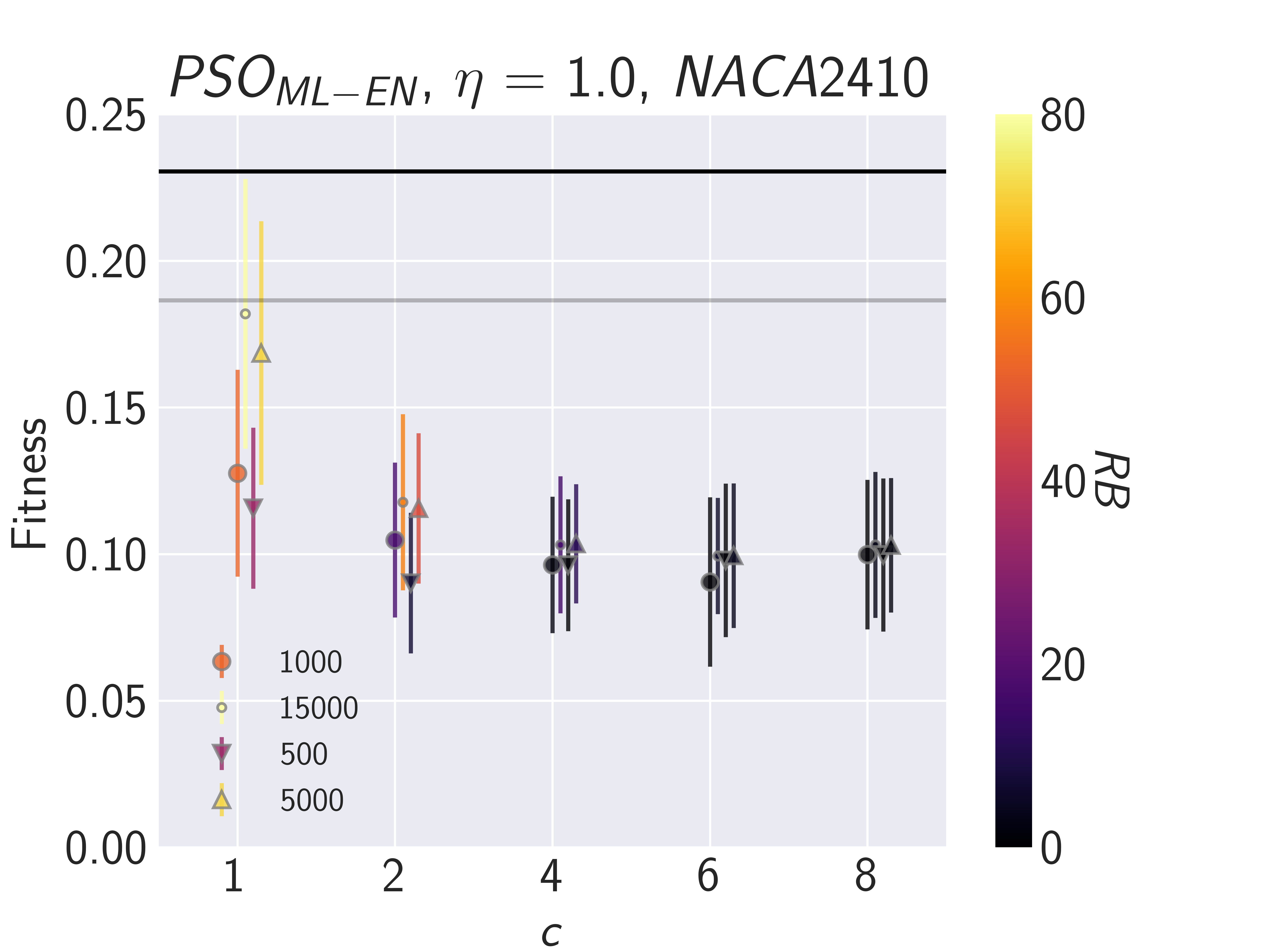
(a)

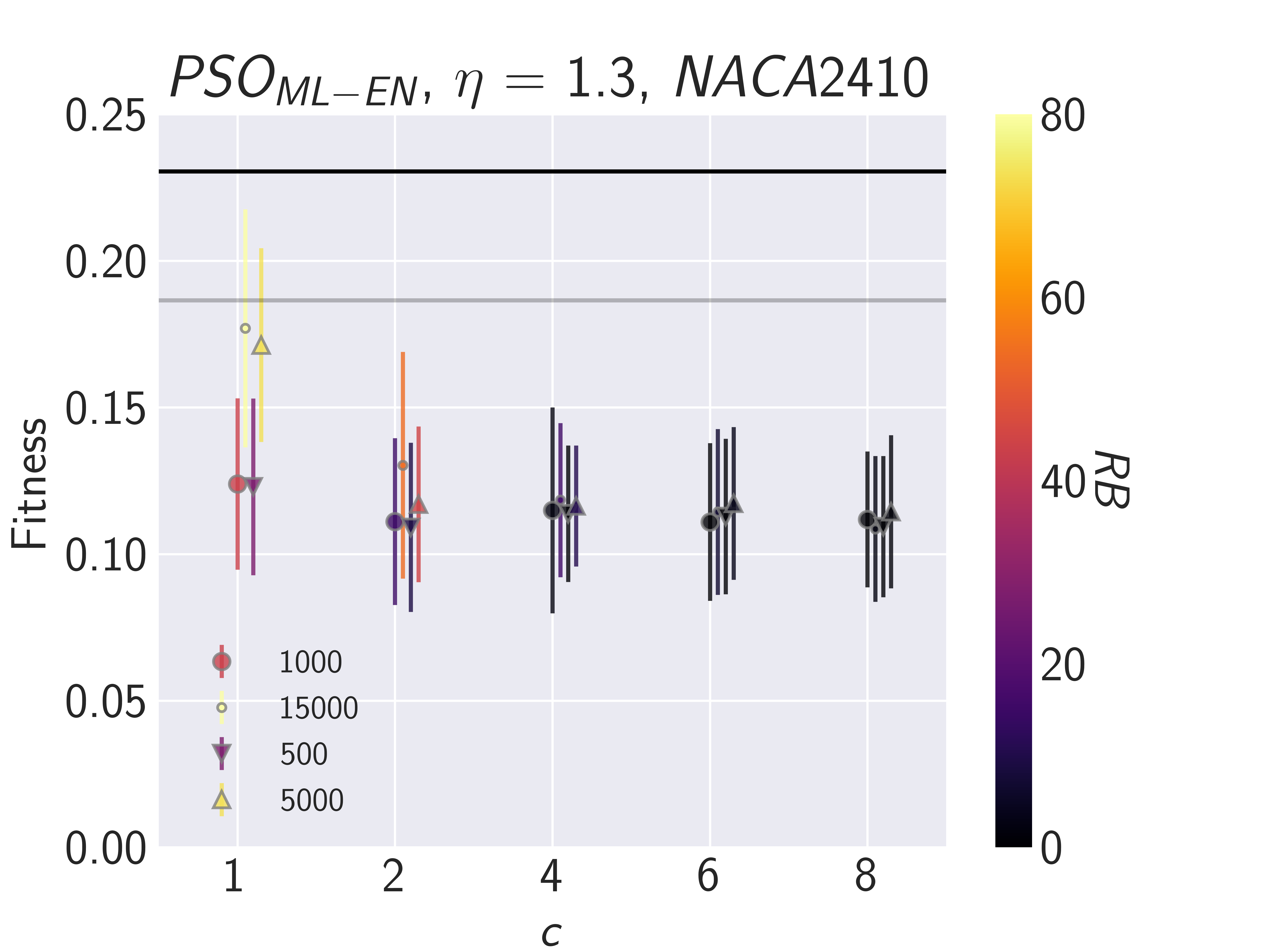
(b)

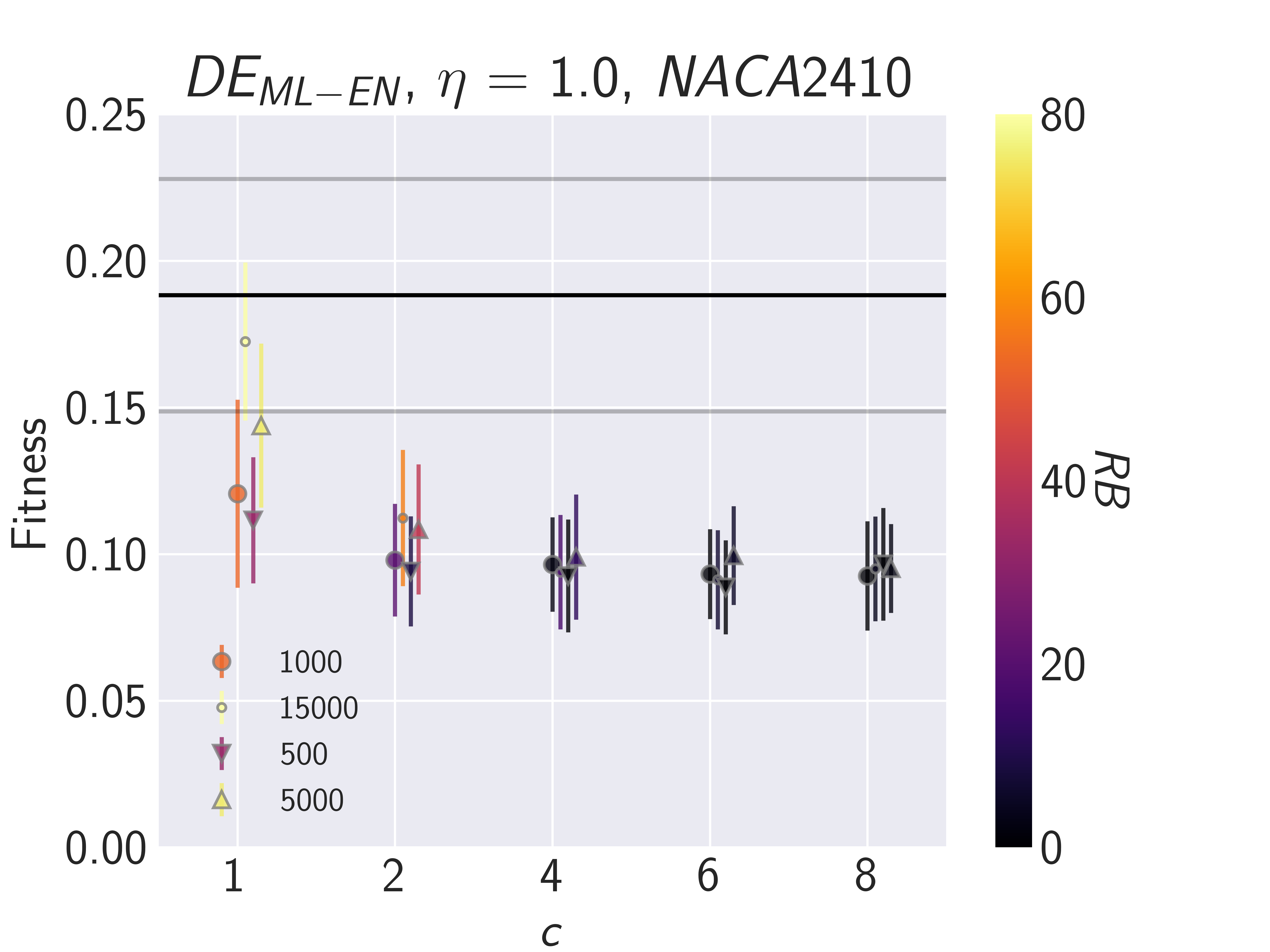
(c)

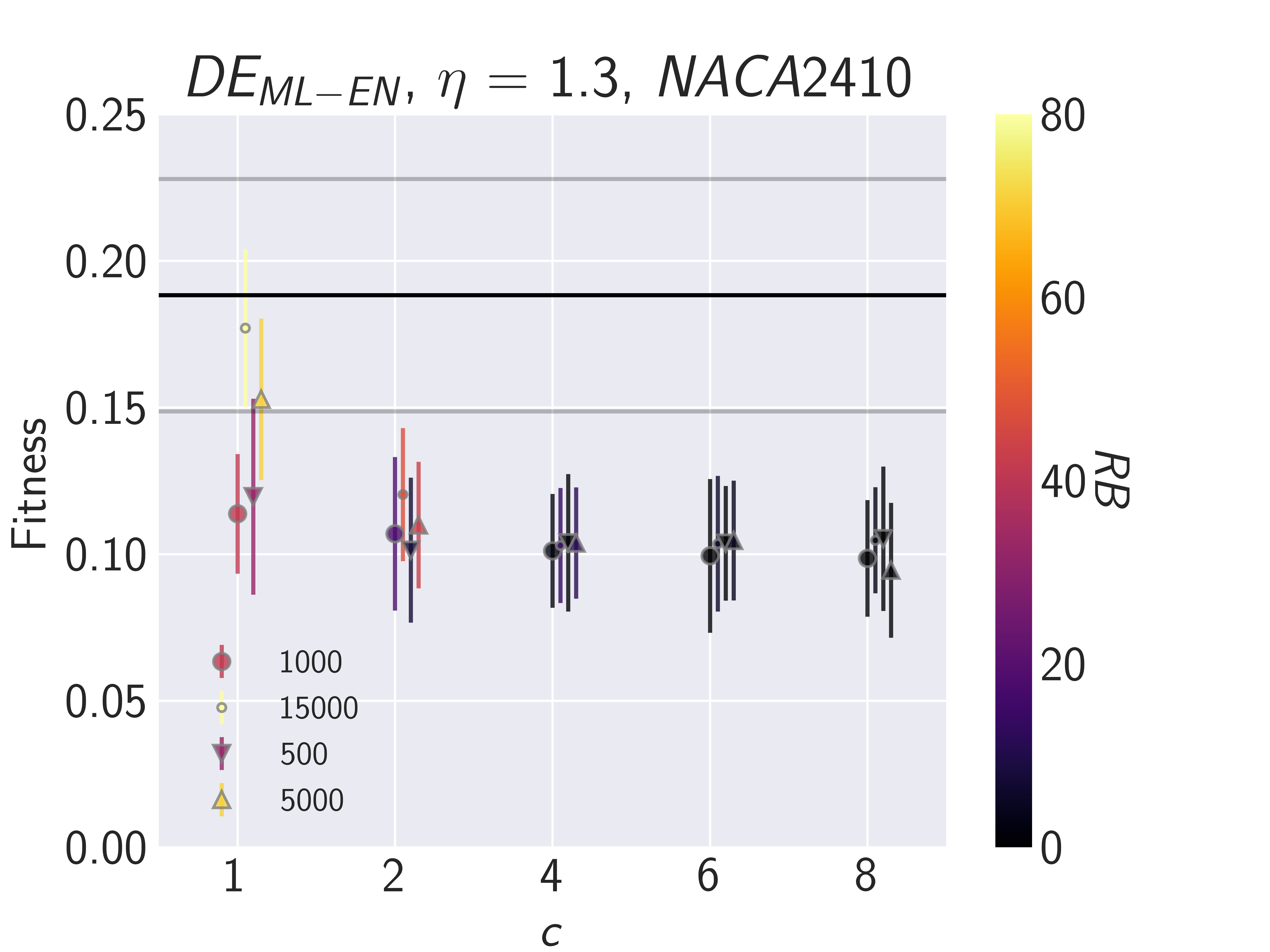
(d)

Figure 13: Results from the ML-enhanced framework for $NACA2410$ that include the search space reduction for the following configurations: (a) $PSO_{ML-EN}$, $\eta$ = 1 (b) $PSO_{ML-EN}$, $\eta$ = 1.3 (c) $DE_{ML-EN}$, $\eta$ = 1 (d) $DE_{ML-EN}$, $\eta$ = 1.3. The markers denote the different dataset sizes used to train the ML model, while the coloring of the markers represents the remaining simulation budget ($RB$) values. A higher $RB$ signifies greater savings in the computational budget (less requirements for HF simulations), while low fitness values imply a better approximation of the target performance. The markers are slightly offset for each $c$ value to improve visibility.

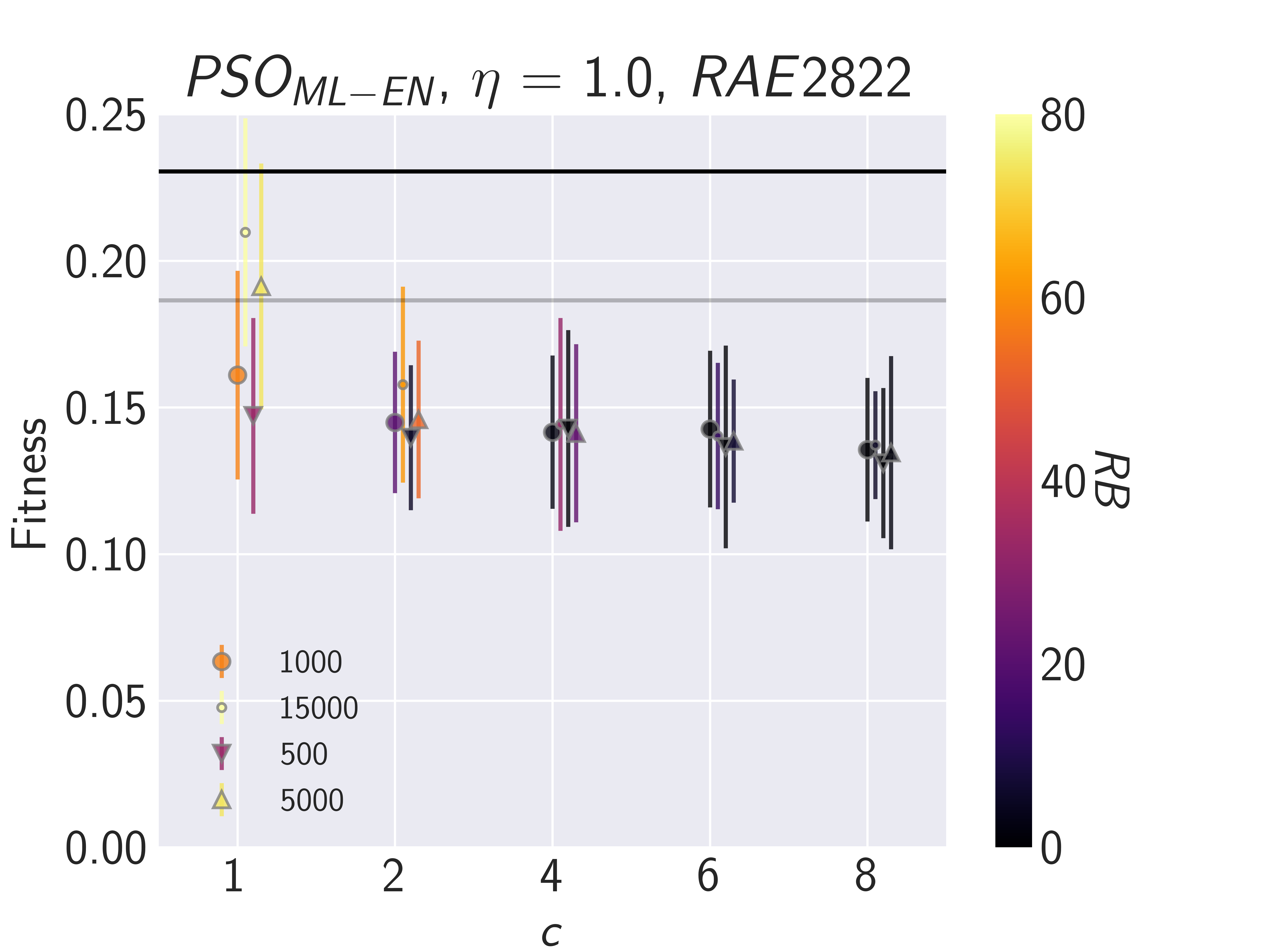
(a)

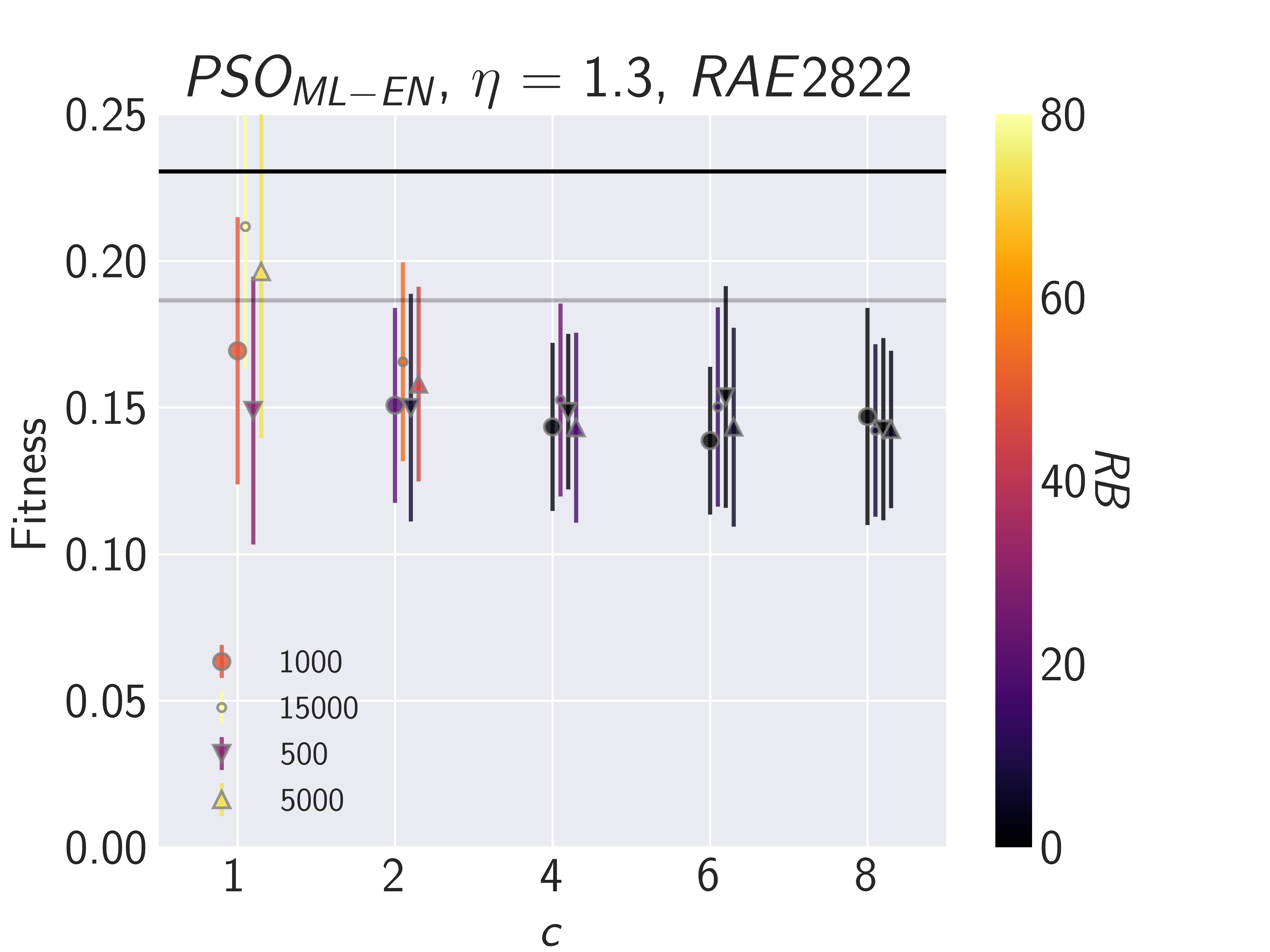
(b)

(c)

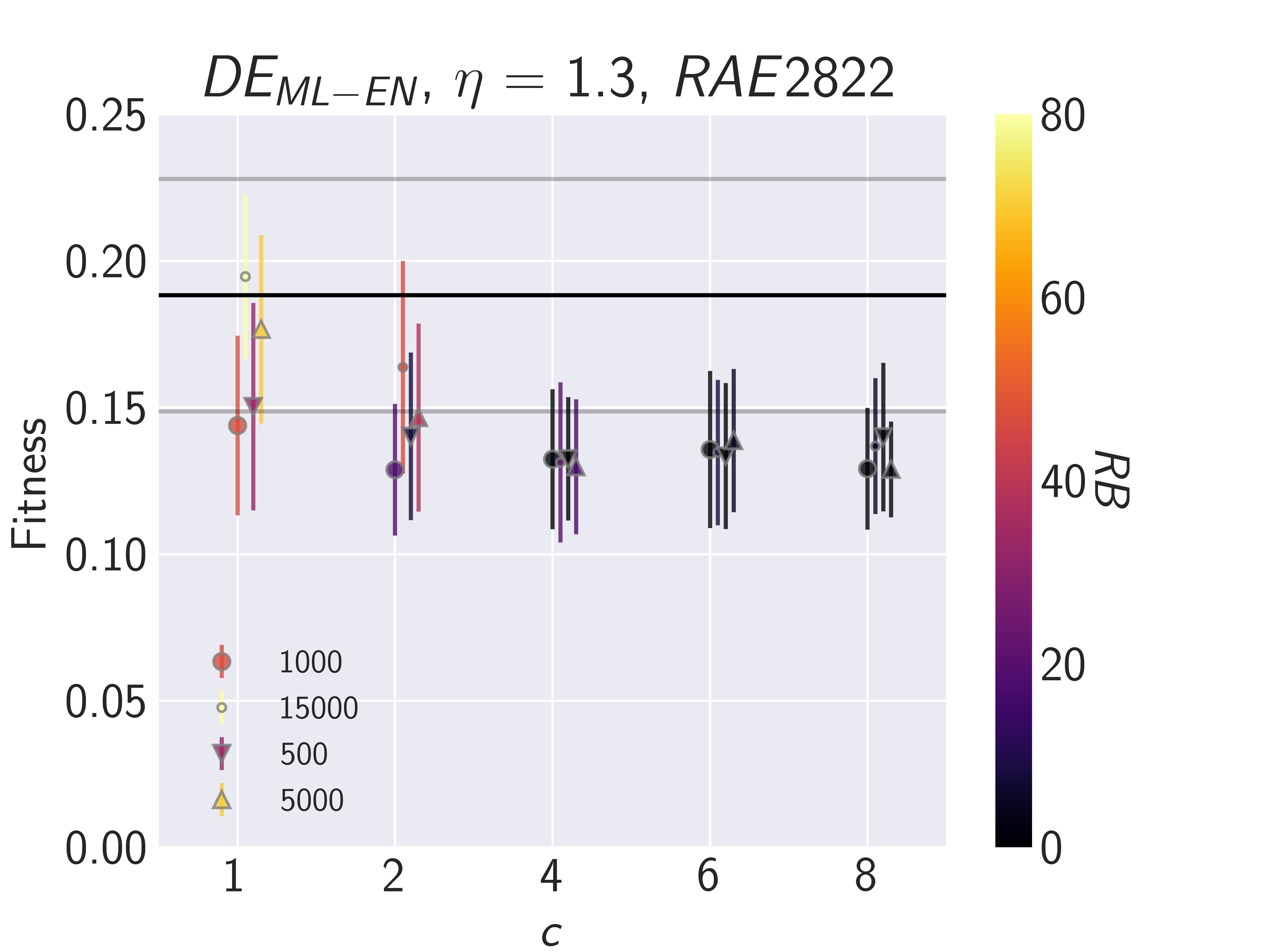
(d)

Figure 14: Results from the ML-enhanced framework for $RAE2822$ that include the search space reduction for the following configurations: (a) $PSO_{ML-EN}$, $\eta$ = 1 (b) $PSO_{ML-EN}$, $\eta$ = 1.3 (c) $DE_{ML-EN}$, $\eta$ = 1 (d) $DE_{ML-EN}$, $\eta$ = 1.3. The markers denote the different dataset sizes used to train the ML model, while the coloring of the markers represents the remaining simulation budget ($RB$) values. A higher $RB$ signifies greater savings in the computational budget, while low fitness values imply a better approximation of the target performance. The markers are slightly offset for each $c$ value to improve visibility.

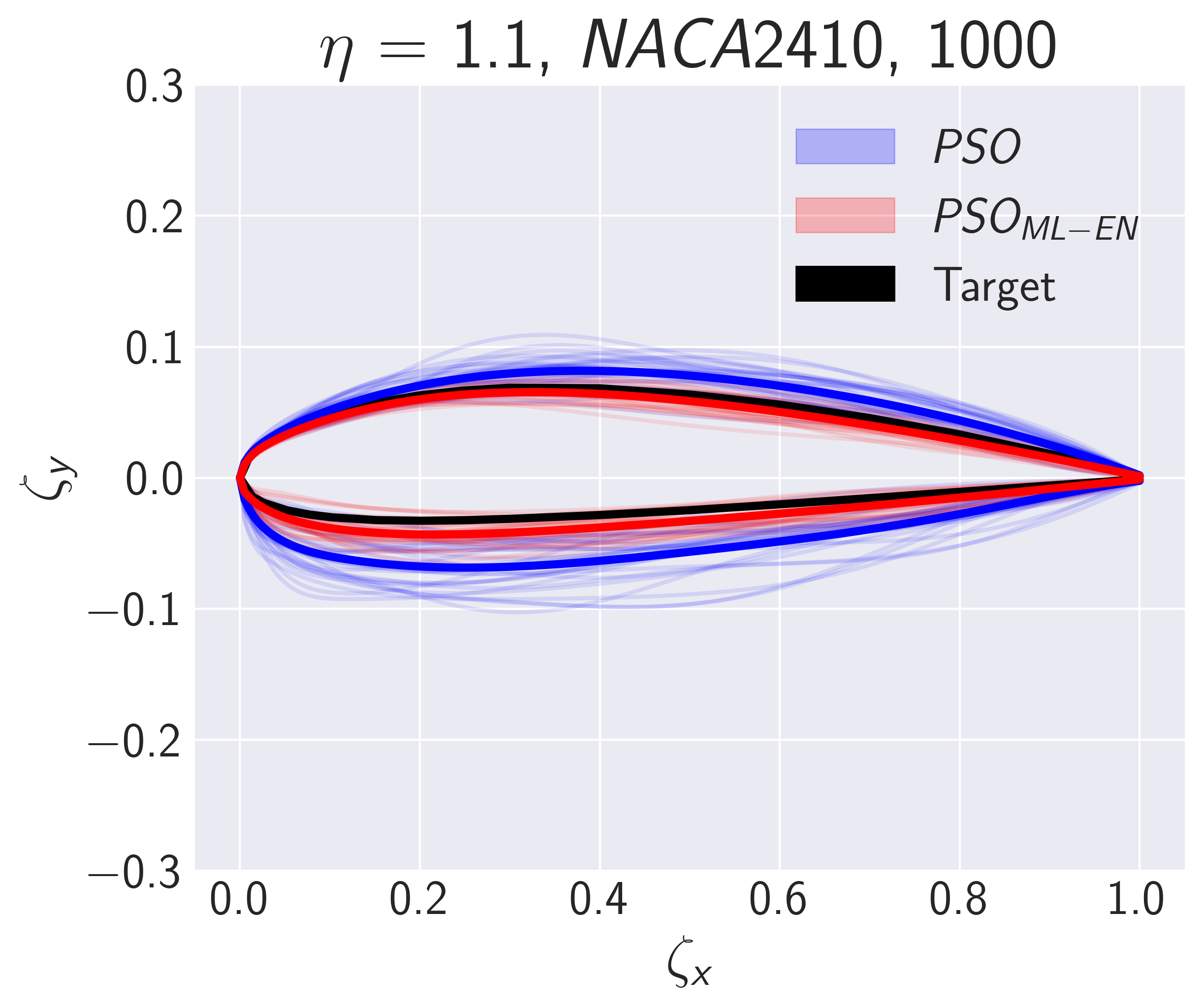
(a)

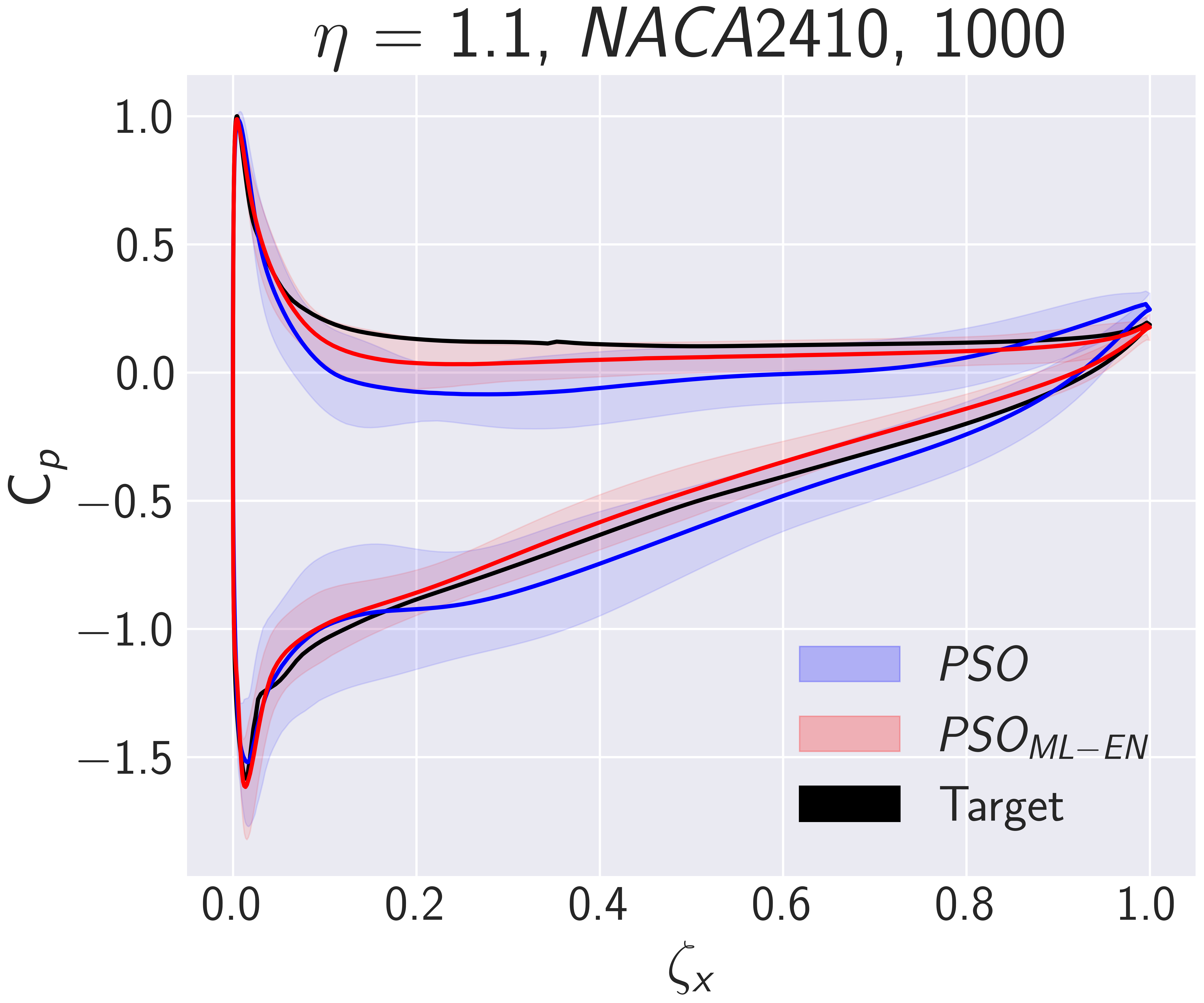
(b)

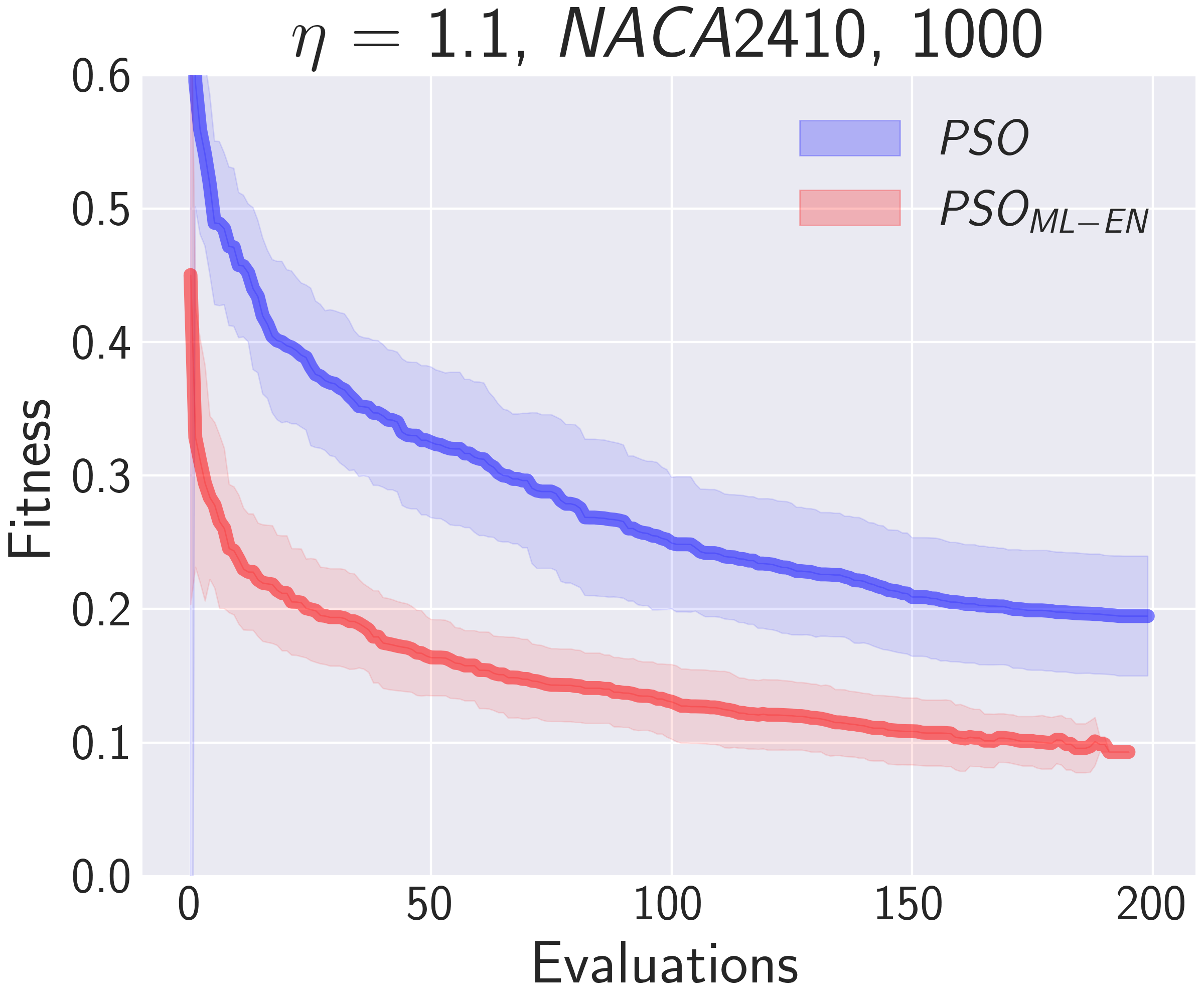
(c)

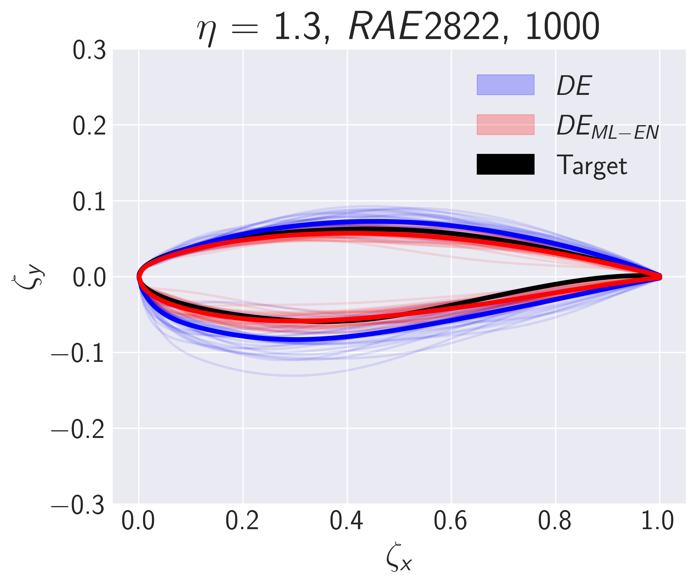
(d)

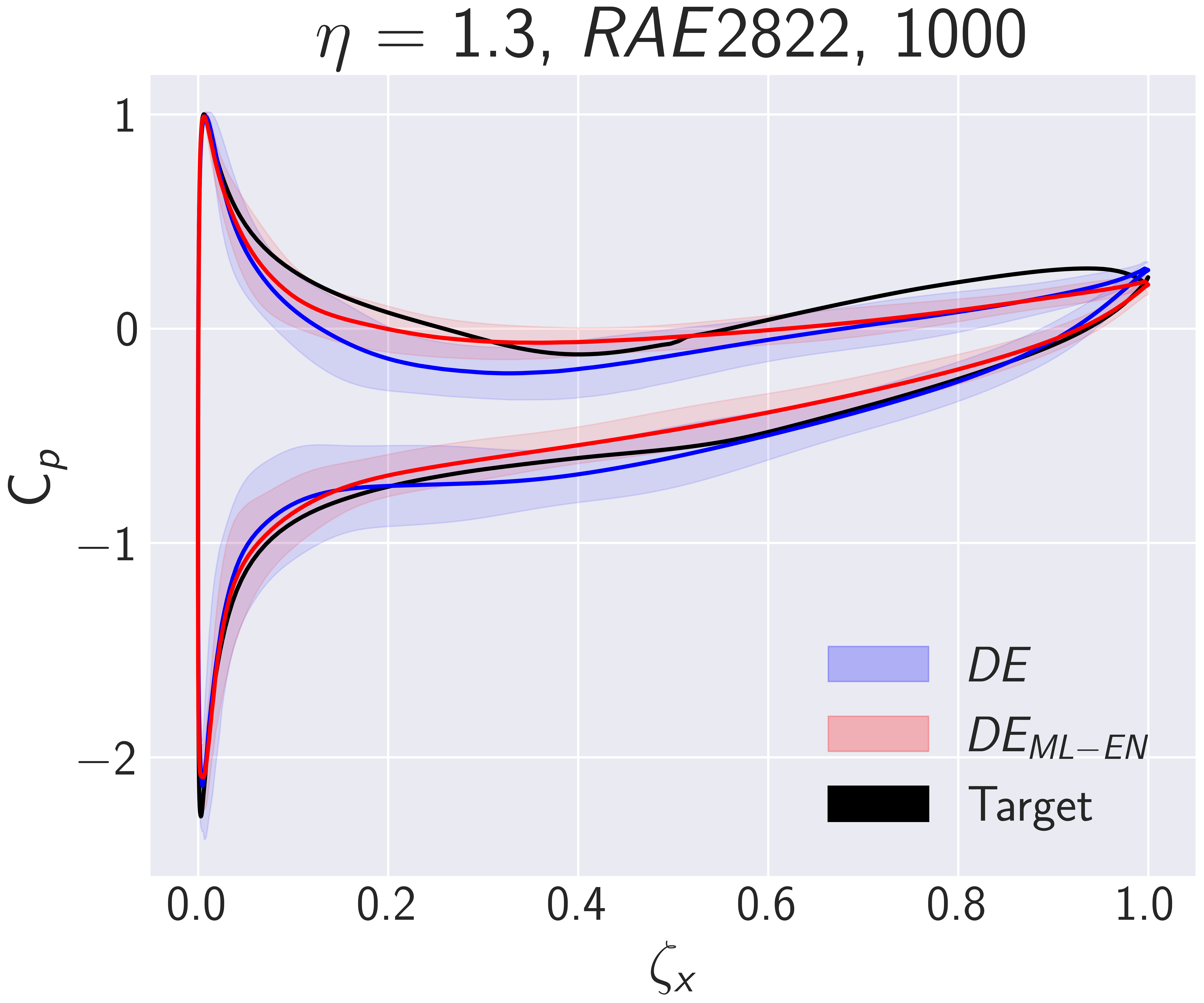
(e)

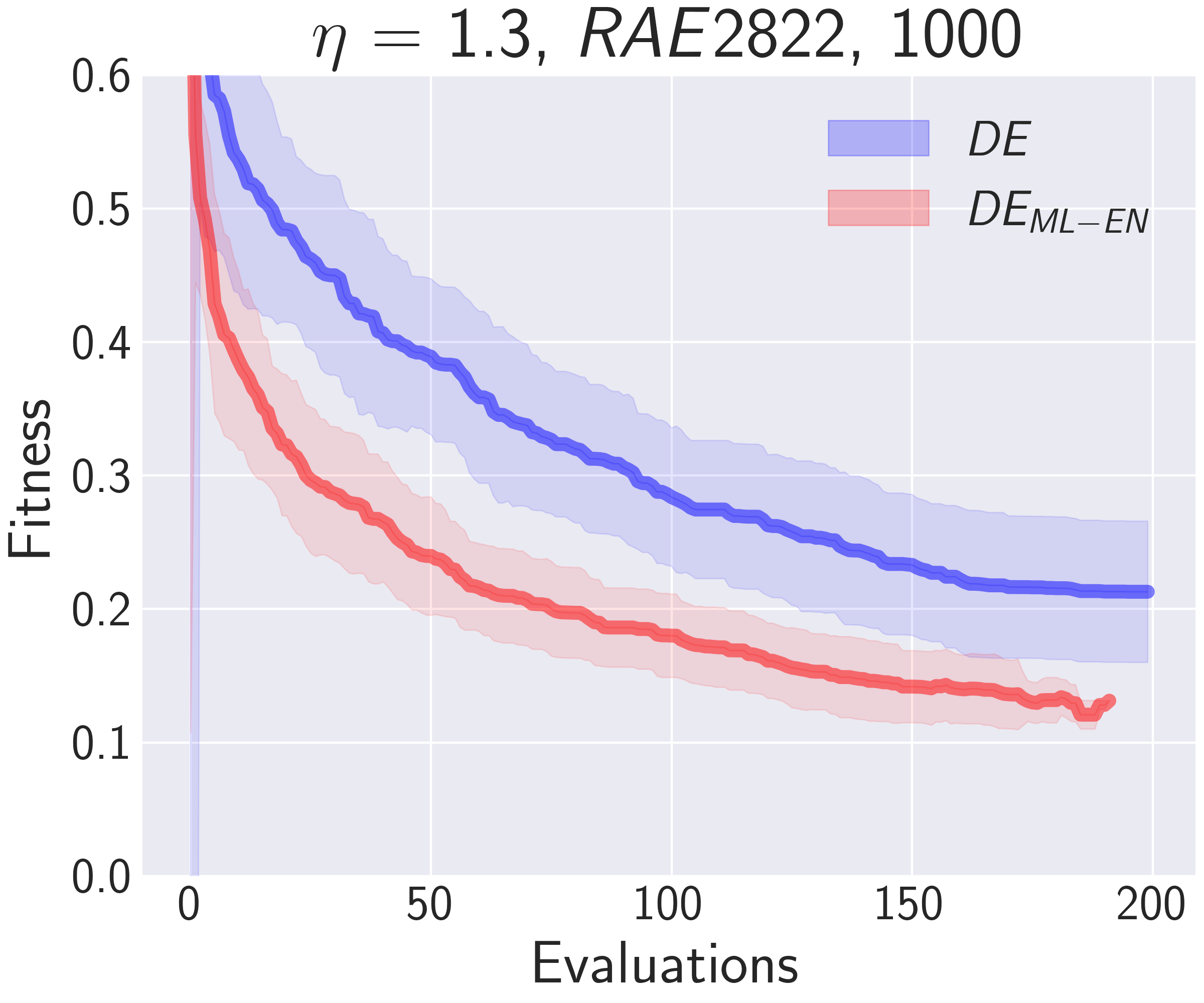
(f)

Figure 15: A comparative analysis of ML-enhanced algorithm configurations (dataset size = 1000 for both rows, $\eta$ = 1.1 for top and $\eta$ = 1.3 for bottom row, respectively) versus their unenhanced optimization equivalents: (a) Optimal achieved $NACA2410$ airfoil geometry for the PSO and $PSO_{ML-EN}$ (b) Optimal set of pressure coefficients for the same configuration juxtaposed with target values (c) Convergence of all 30 runs for PSO and $PSO_{ML-EN}$ (d) Optimal achieved $RAE2822$ airfoil geometry for DE and $DE_{ML-EN}$ (e) Corresponding optimal pressure coefficients set against target values for the $RAE2822$ airfoil (f) Average convergence and standard deviation of all 30 runs for both algorithm variants. The thicker lines in the first and second column represent the average optimized designs and pressure coefficients from the 30 runs, while the transparent shaded region in the second column depicts the standard deviation of the pressure coefficients.

6.3.2 SFR Results

Fig. 16 presents the hyperparameter analysis for the ML-framework applied to the SFR problem. It also provides a comparison with the unenhanced algorithms showing the average and standard deviation of the fitness, indicated by the horizontal black and grey lines, respectively. The ML-enhanced algorithms consistently outshine their traditional counterparts. Drawing parallels with the AID problem, it is observed that while elevating the $c$ parameter allows the framework to focus on improving the target performance approximation (reducing the fitness value), it does so at the expense of fully utilizing the entire simulation budget.

The ML-enhanced optimizers with the MLP model trained on the dataset size 1000 exhibit superior performance in terms of fitness value compared to their counterparts trained on dataset sizes 500 and 5000, respectively. This difference can be attributed to the more effective search space reduction achieved by the 1000-instance model, as evidenced by Figures 12(a) and 12(b). The applied search space reduction notably contributes to reducing fitness uncertainty across all hyperparameter combinations as observed through the standard deviation lines corresponding to each marker. This advantage becomes even more pronounced when compared to the standard deviation observed in the unenhanced algorithms.

For dataset sizes of 500 and 1000, a $c$ value of 1 or greater causes the ML-enhanced algorithms to consume the entire budget of HF simulations. Notably, when optimizers are paired with the MLP model trained on 5000 instances, the fitness scales almost linearly with the $c$ value. The 5000-instance trained ML-enhanced optimizers strike an good trade-off between achieving low fitness ($RMSE$) values and conserving HF simulations. Considering results from both BC scenarios, the hyperparameter settings that would achieve a trade-off between a good target performance approximation and simulation budget would be the 1000 dataset model at $c$ = 0.25 or the 5000 dataset model at $c$ = 1. If the goal is to substantially narrow down the design space, a noisy model, like the one trained on 500 instances, proves sufficient.

Fig. 17 displays examples of the optimized BCs for both test instances. The results from PSO_ML-EN for the sinusoidal BC employed an MLP trained on 1000 instances with $c$ = 1, while for the linear BC an MLP trained on 500 instances with $c$ = 1 was used. Different reconstructed averaged BCs are depicted for both instances and algorithms. This variety arises because the final optimized average design vectors, which contained raw scalar values for each $\Omega_{top}$ coordinate, underwent regression model fitting ranging from degrees 1 to 4, described in Sect. 4.2. In both cases presented in Fig. 17, both the average reconstructed BCs (for all regression model degrees) and the convergence plot clearly demonstrate the superiority of PSO_ML-EN over PSO.

In Fig. 18, the reconstructed scalar fields generated by the BCs presented in Fig. 17 are shown. The top row shows the fields for the sinusoidal BC, while the bottom row shows the fields for the linear BC. The first column shows the ground truth, while the second and third columns show the $PSO_{ML-EN}$ and PSO reconstructed scalar fields. It is obvious that the BCs generated by the ML-enhanced algorithm align much more closely with the true solution. Finally, Fig. 19 shows the absolute error between the true scalar fields (for both BC cases) and those obtained by $PSO_{ML-EN}$ and PSO-optimized boundary conditions. The absolute error was calculated for every point in the HF domain, and with the range of the absolute error being the same for both results shown, it is apparent that the $PSO_{ML-EN}$ generated BC is more accurate.

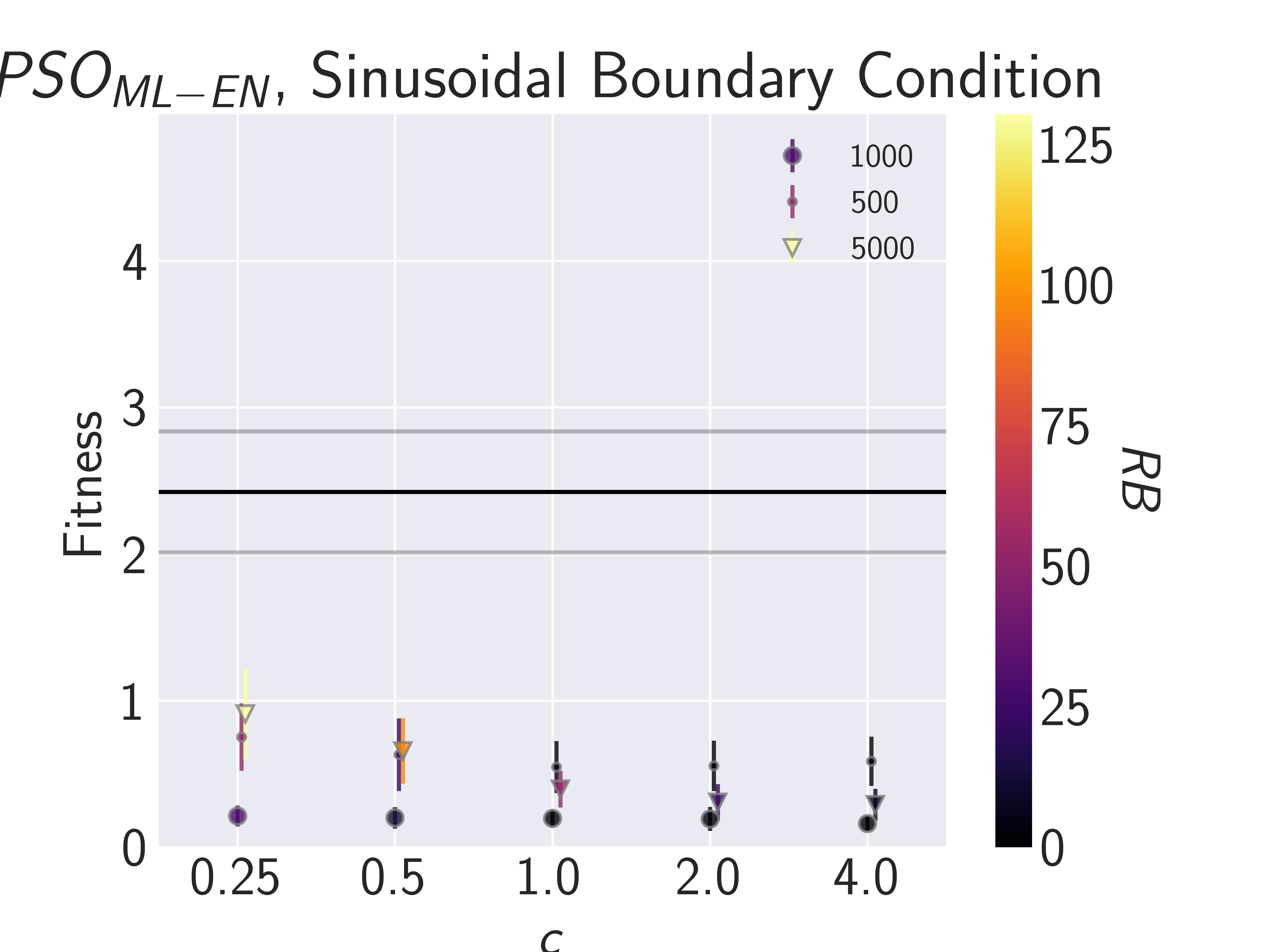
(a)

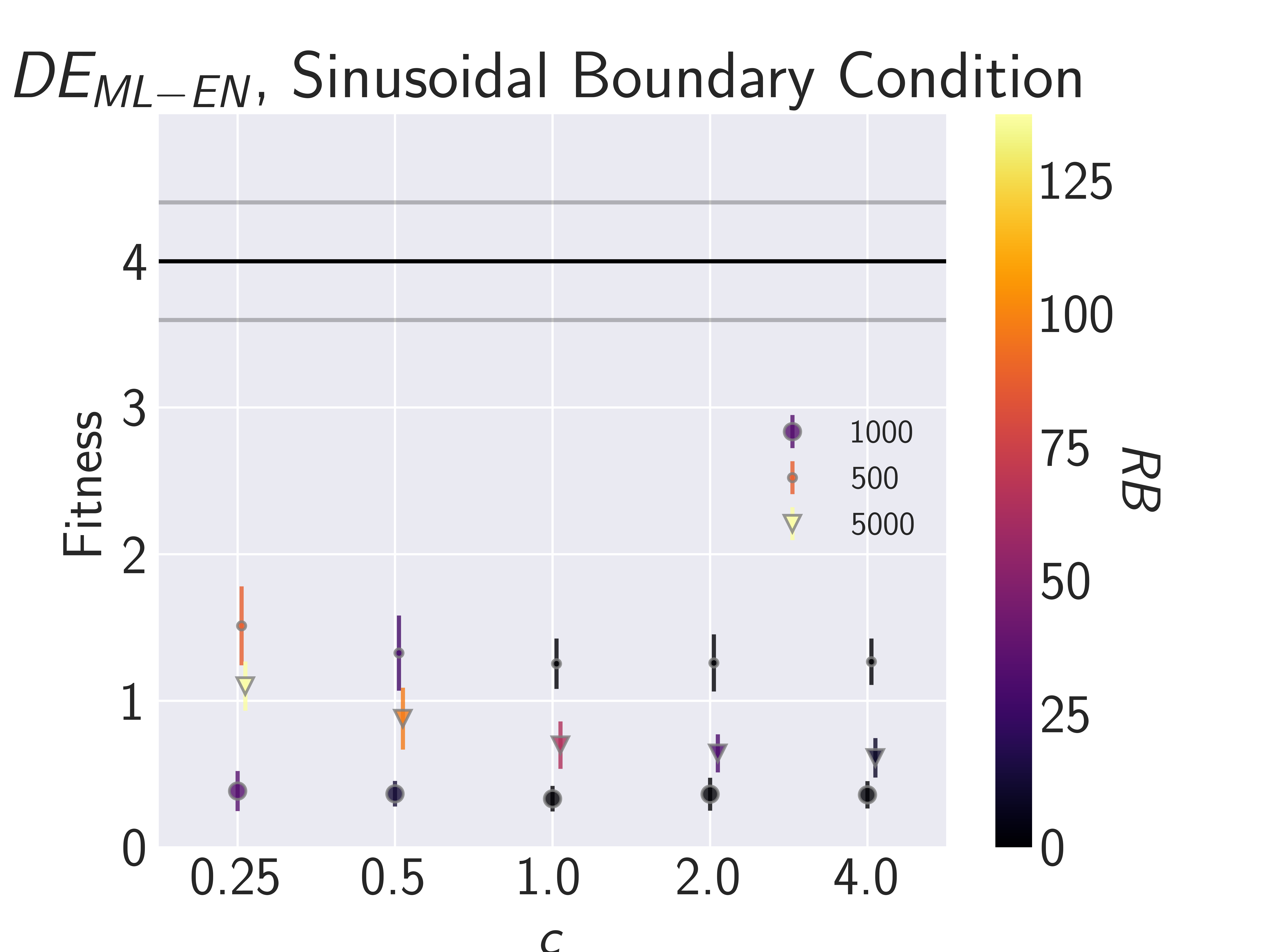
(b)

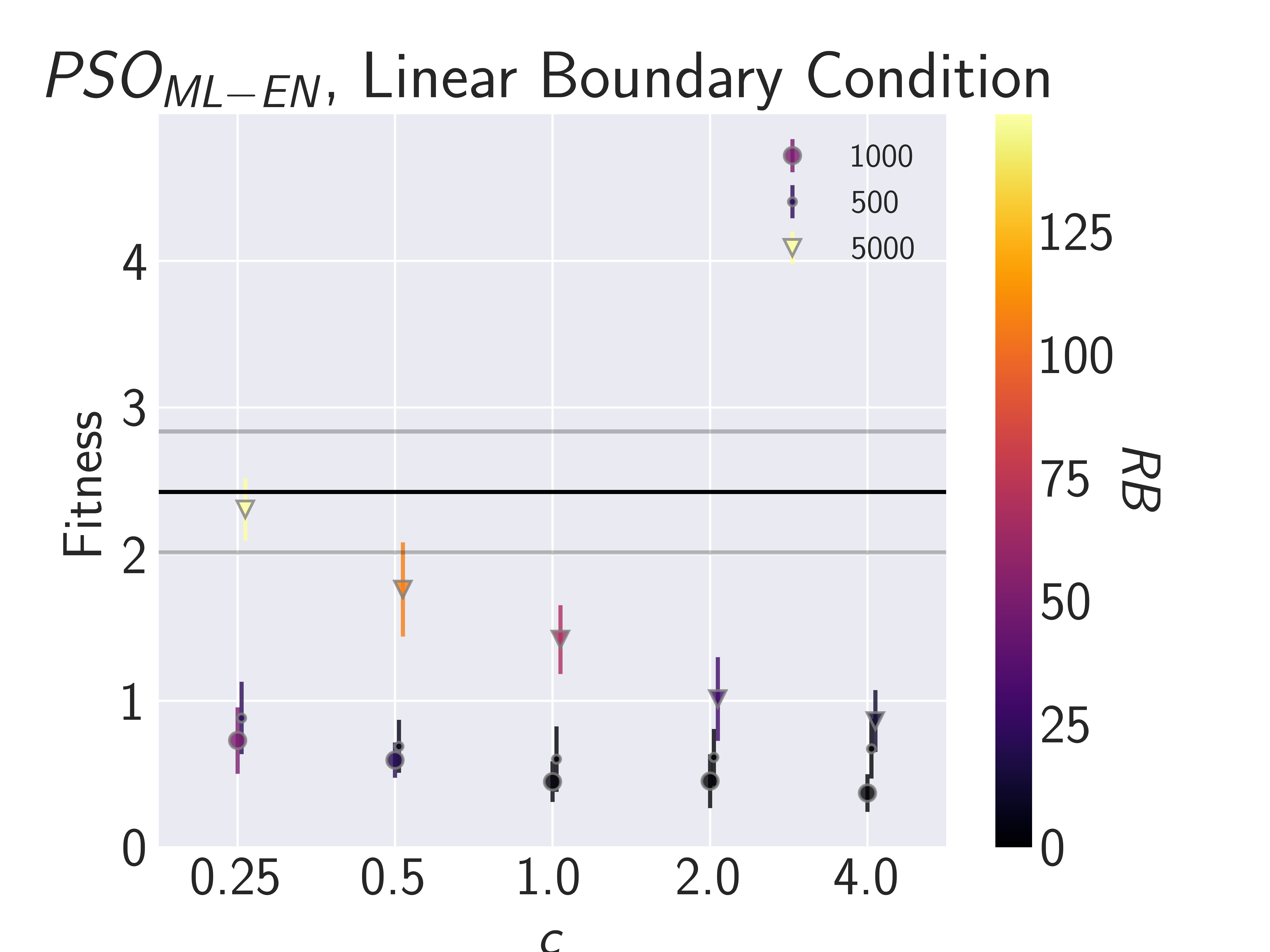
(c)

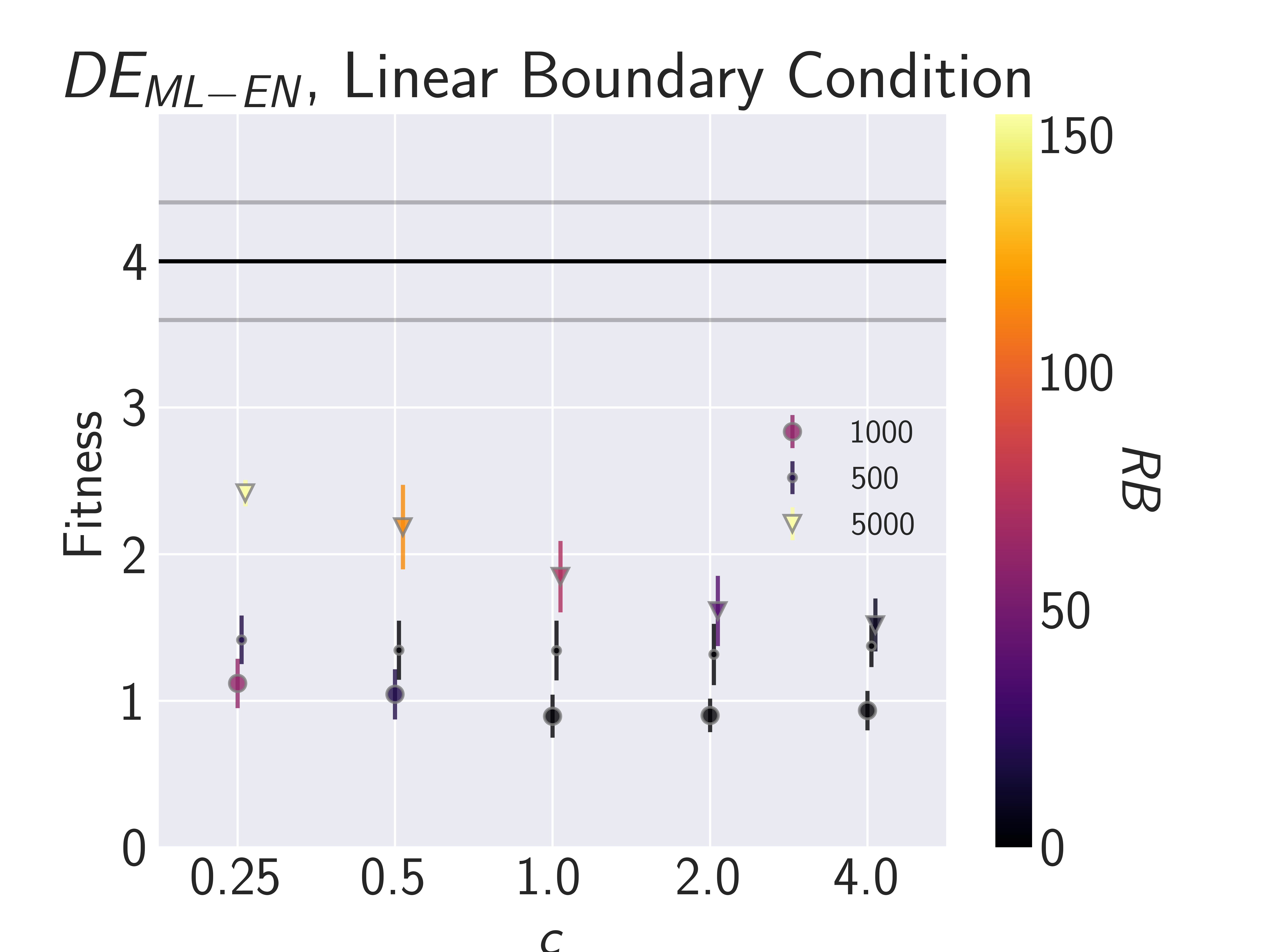
(d)

Figure 16: ML-enhanced framework results for the surface field reconstruction problem: (a) $PSO_{ML-EN}$ for the sinusoidal BC (b) $DE_{ML-EN}$ for the sinusoidal BC (c) $PSO_{ML-EN}$ for the linear BC (d) $DE_{ML-EN}$ for the linear BC. The markers denote the different dataset sizes used to train the ML model, while the coloring of the markers represents the remaining simulation budget ($RB$) values. A higher $RB$ signifies greater savings in the computational budget, while low fitness values imply a better approximation of the target performance. The markers are slightly offset for each $c$ value to improve visibility.

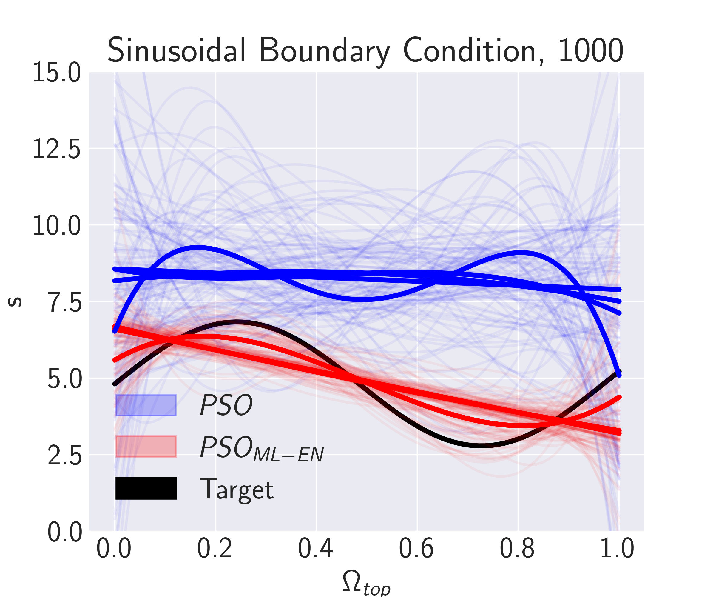
(a)

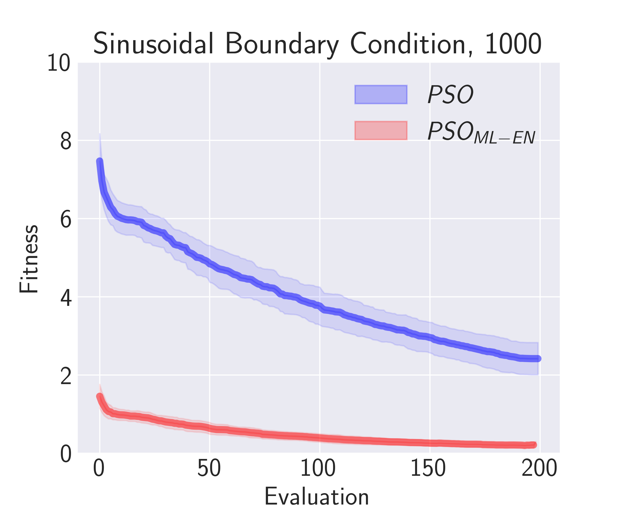
(b)

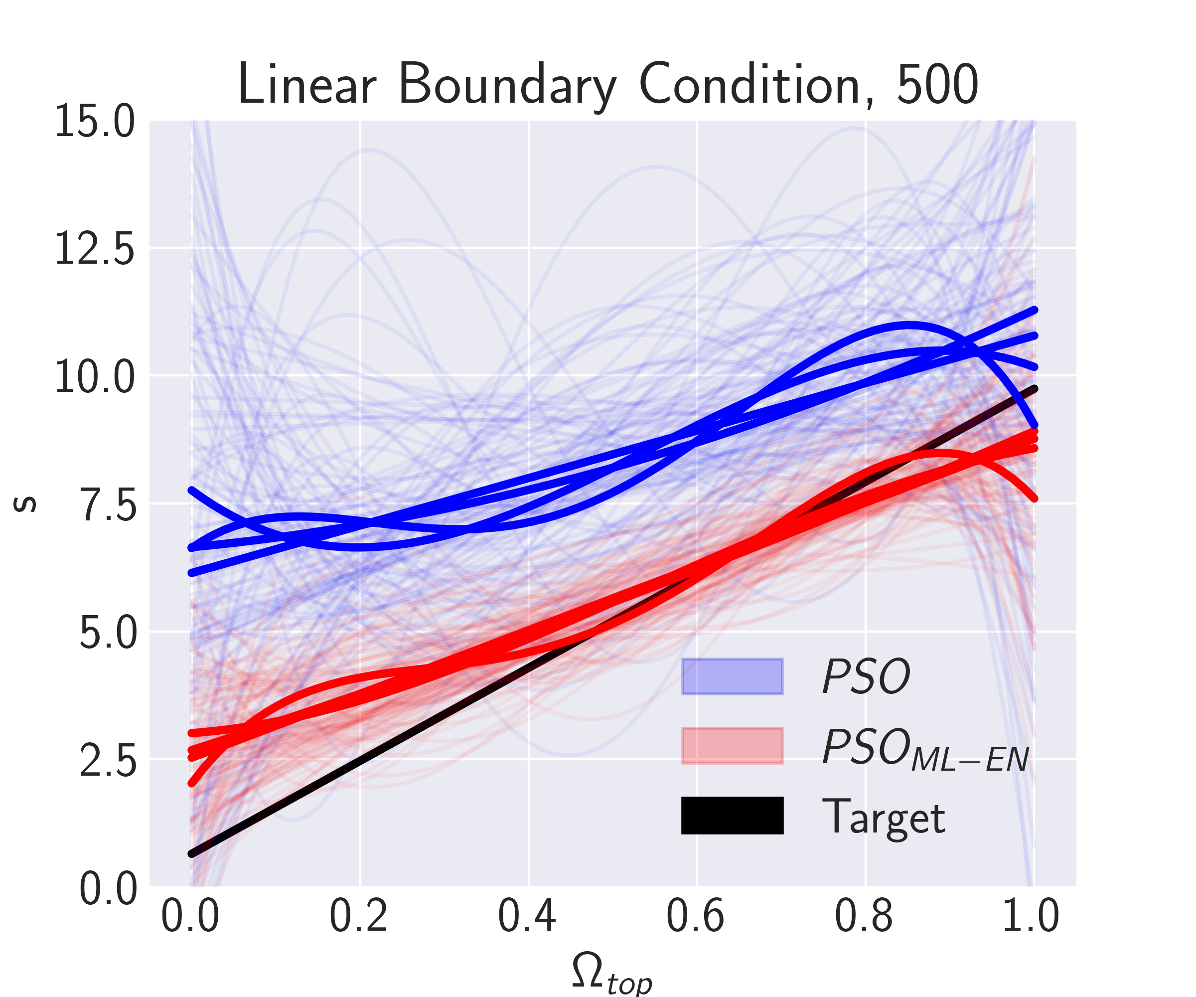
(c)

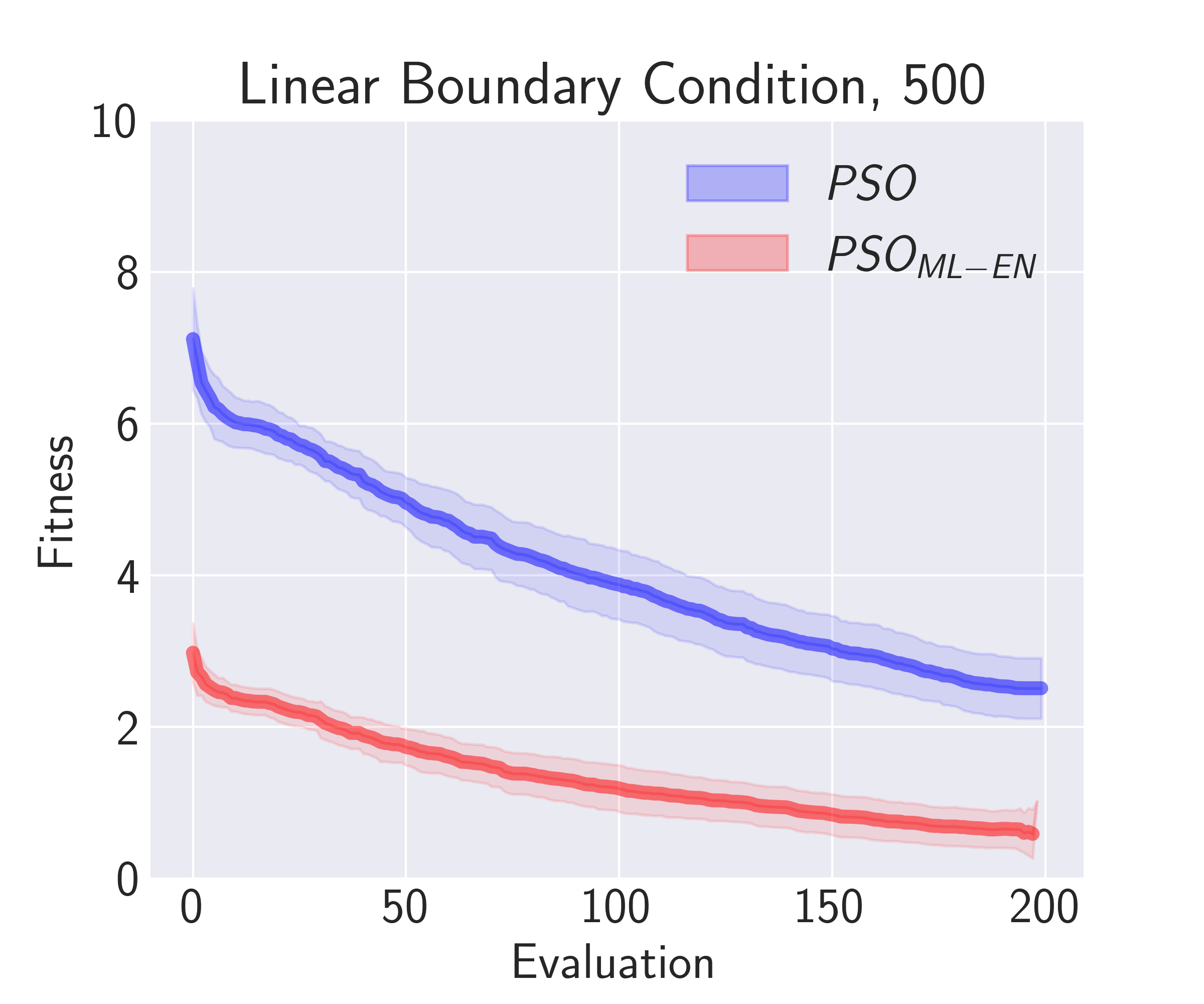
(d)

Figure 17: A comparative analysis of ML-enhanced PSO algorithm configurations with $c$ = 1 (MLP training dataset size = 1000 for top row, and 500 for bottom row) versus their unenhanced optimization equivalents: (a) PSO and $PSO_{ML-EN}$ comparison of the reconstructed sinusoidal BC juxtaposed with the true BC (b) Sinusoidal BC case 30 runs average convergence and standard deviation plot of PSO and $PSO_{ML-EN}$ (c) PSO and $PSO_{ML-EN}$ comparison of the reconstructed linear boundary condition juxtaposed with the true BC (d) Linear BC case 30 runs average convergence and standard deviation plot of PSO and $PSO_{ML-EN}$. The thicker lines in the first column represent the average BCs of the 30 runs. There are four thicker lines shown since the solutions were approximated with four different degrees of regression.

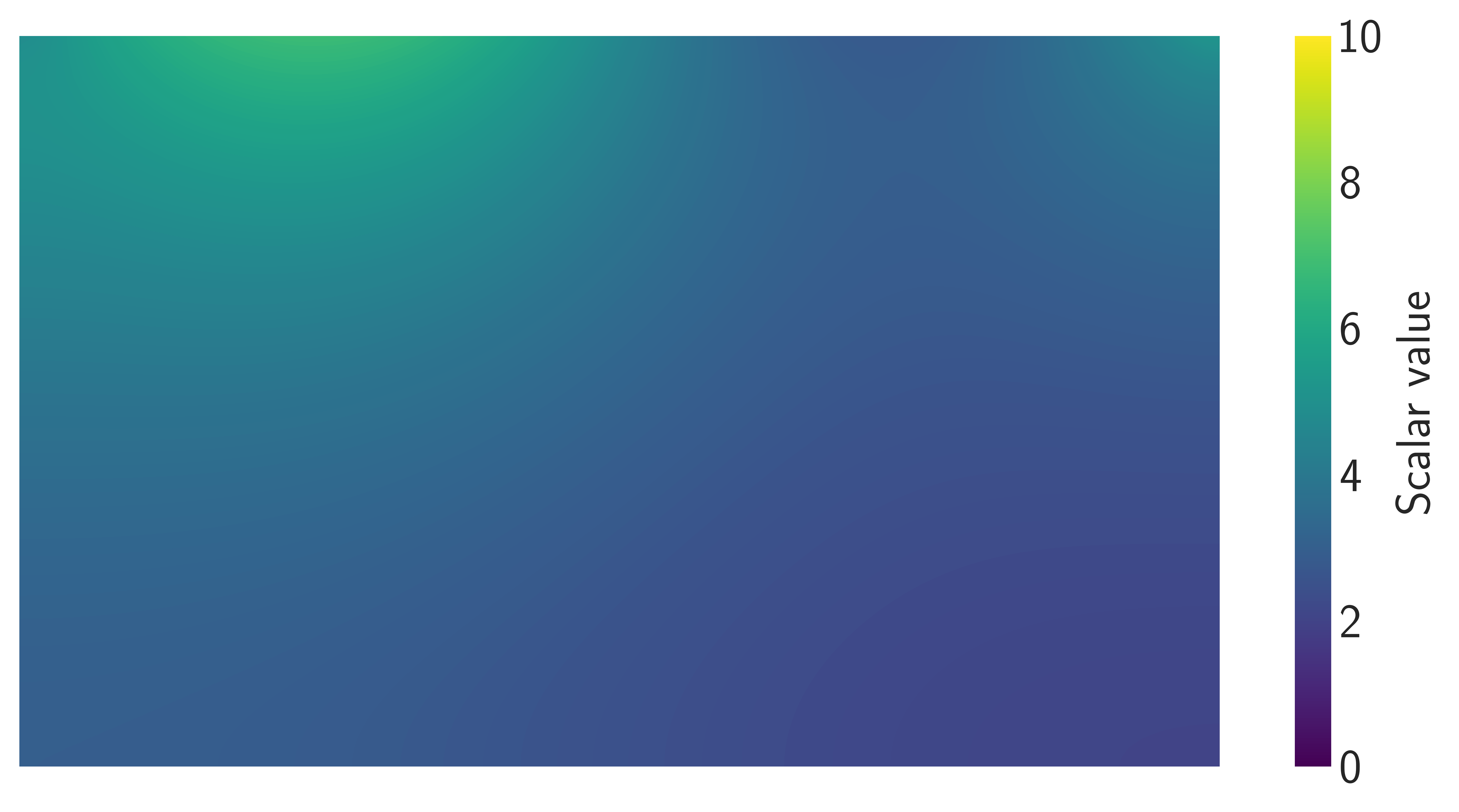
(a)

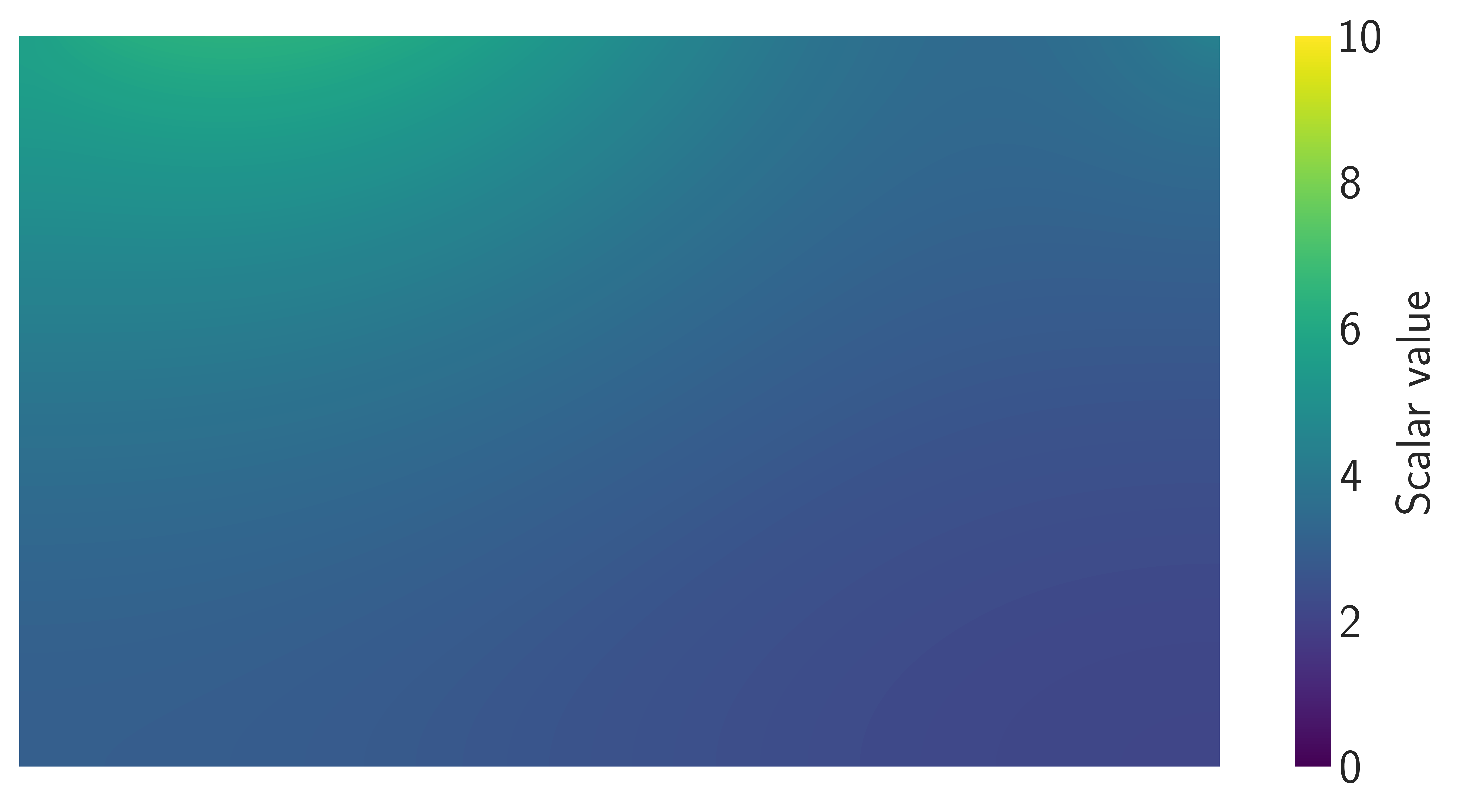
(b)

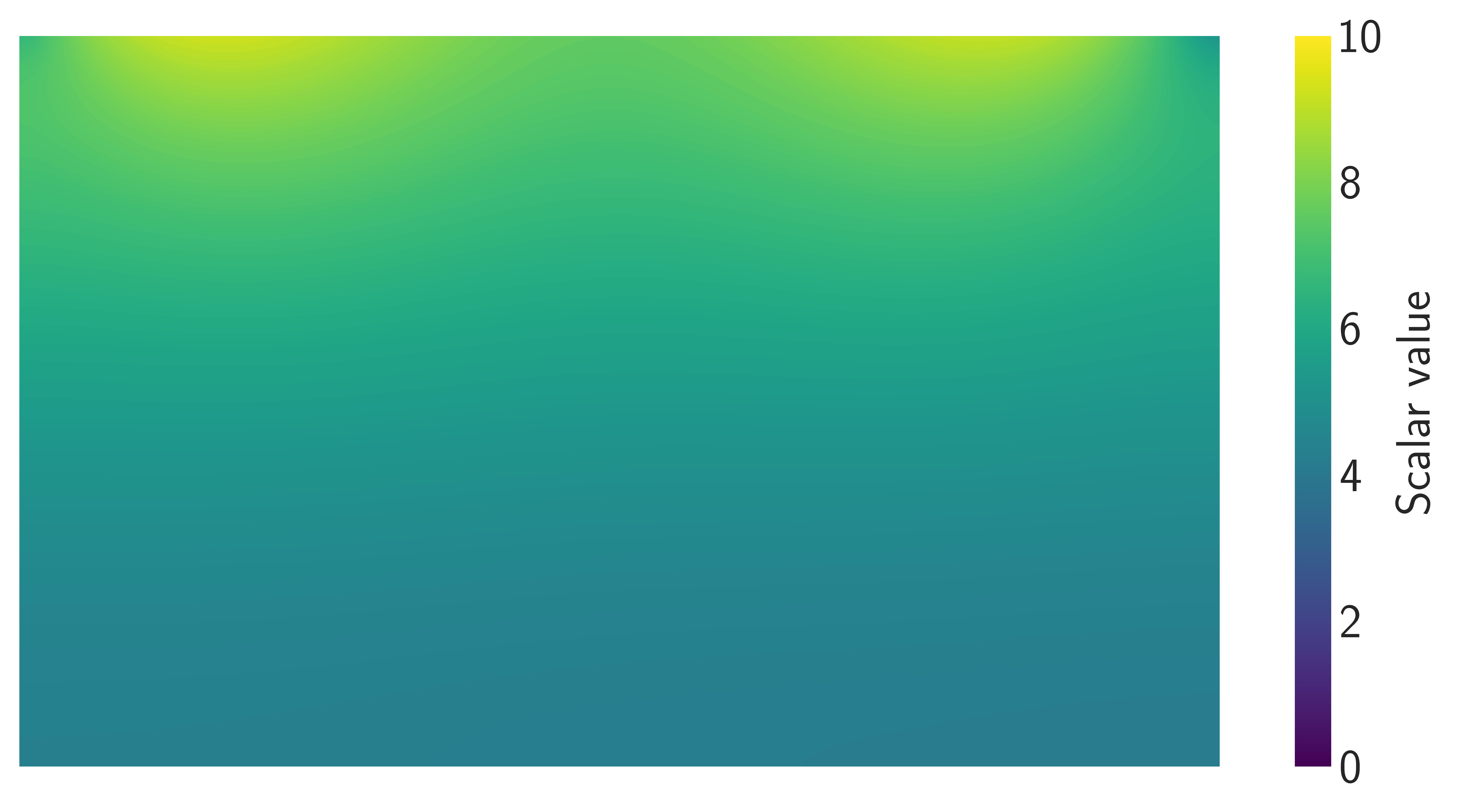
(c)

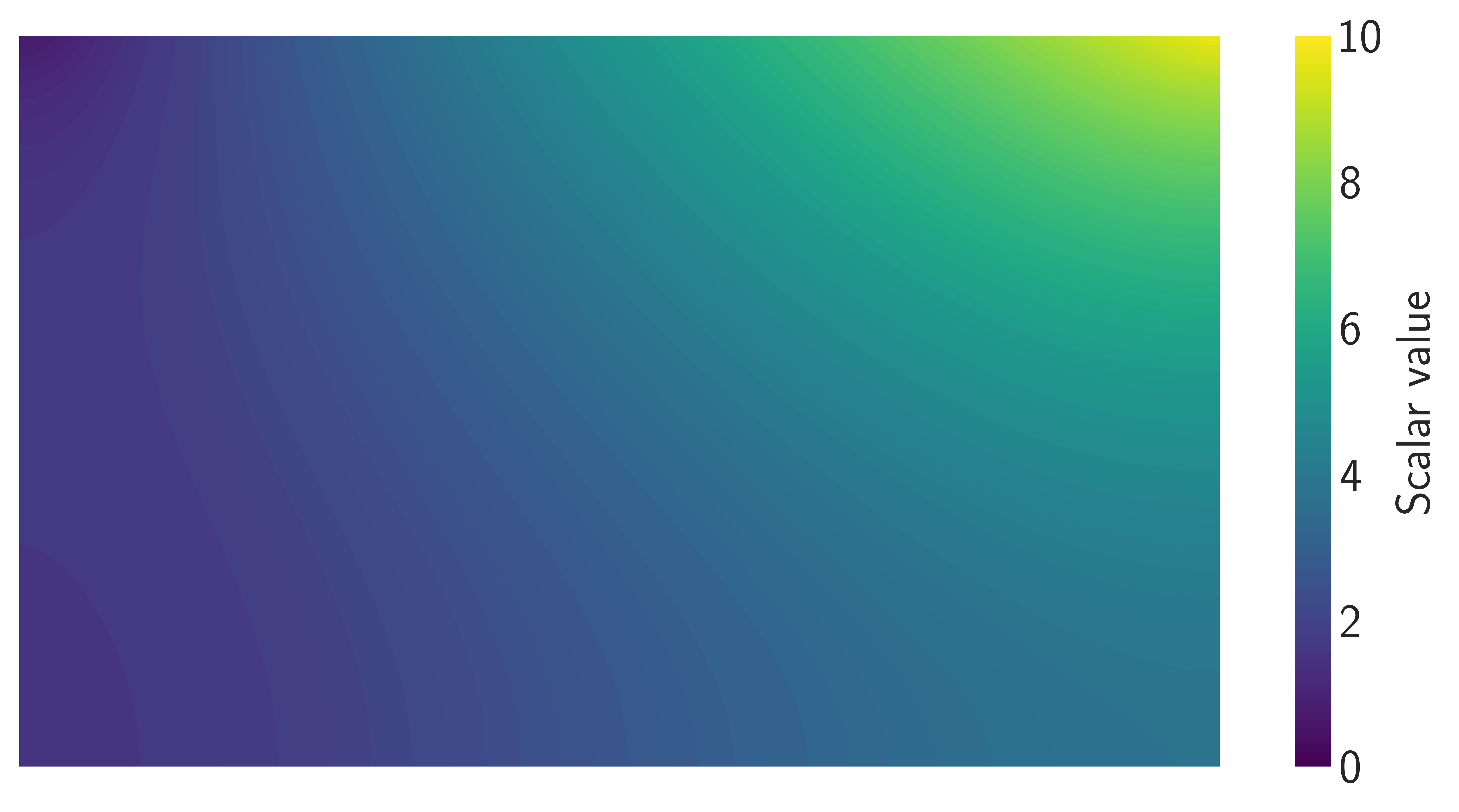
(d)

(e)

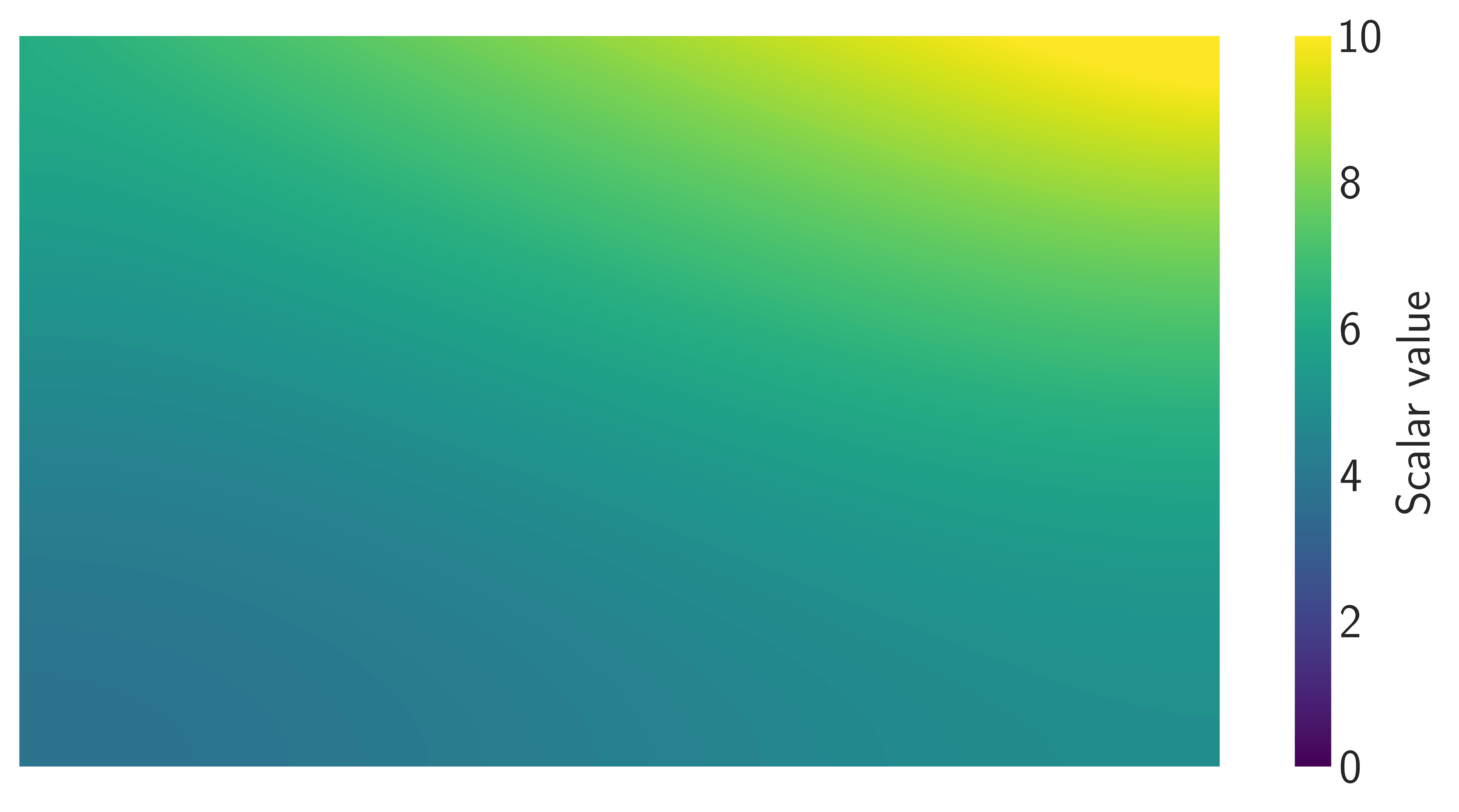
(f)

Figure 18: Reconstructed scalar fields with the average optimized design vectors presented in Fig. 17: (a) True sinusoidal boundary condition (b) $PSO_{ML-EN}$ reconstructed sinusoidal boundary condition (4-th degree regression model) (c) PSO reconstructed sinusoidal boundary condition (4-th degree regression model) (d) True linear boundary condition (e) $PSO_{ML-EN}$ reconstructed linear boundary condition (linear regression model) (f) PSO reconstructed linear boundary condition (linear regression model).

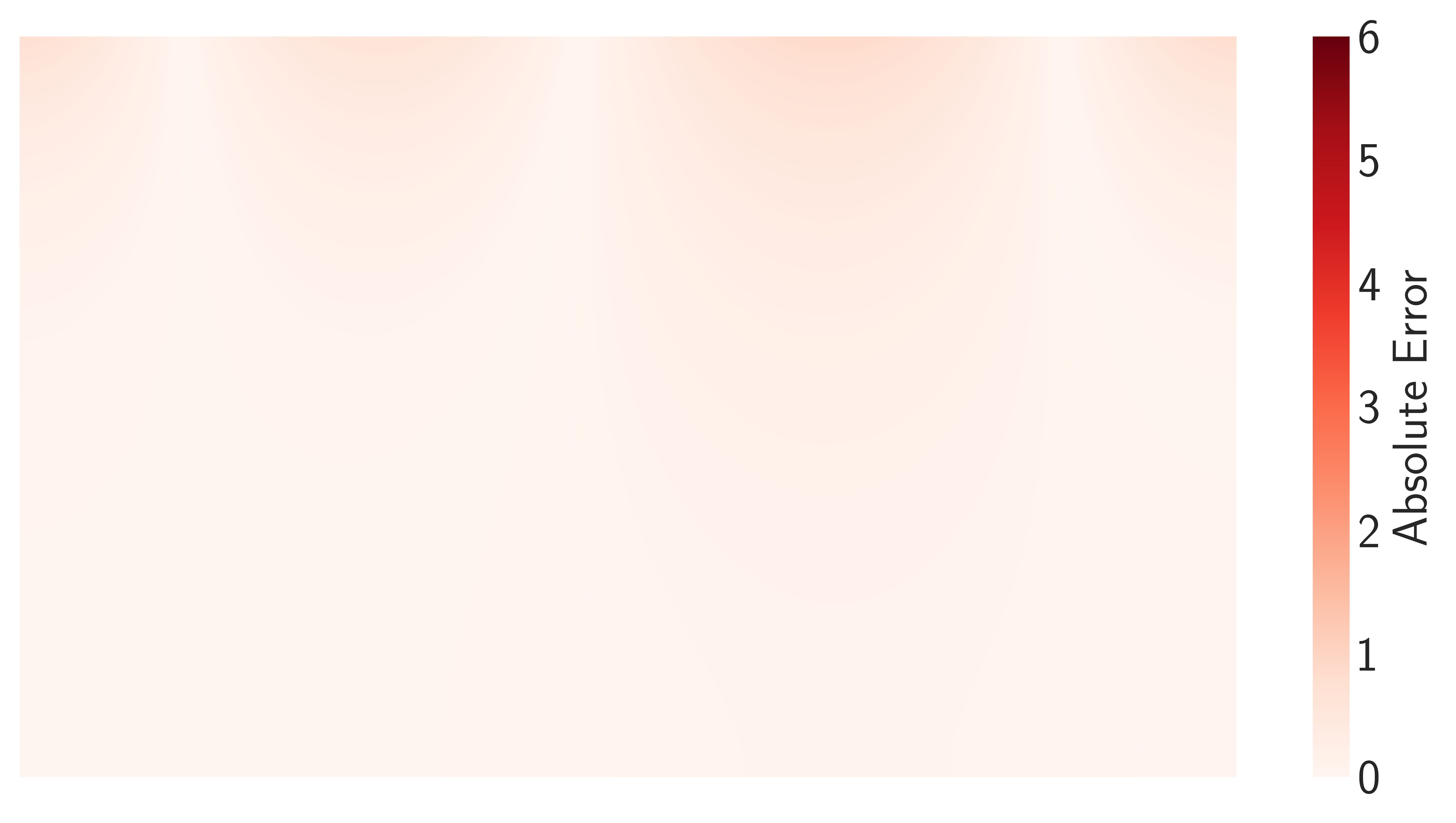
(a)

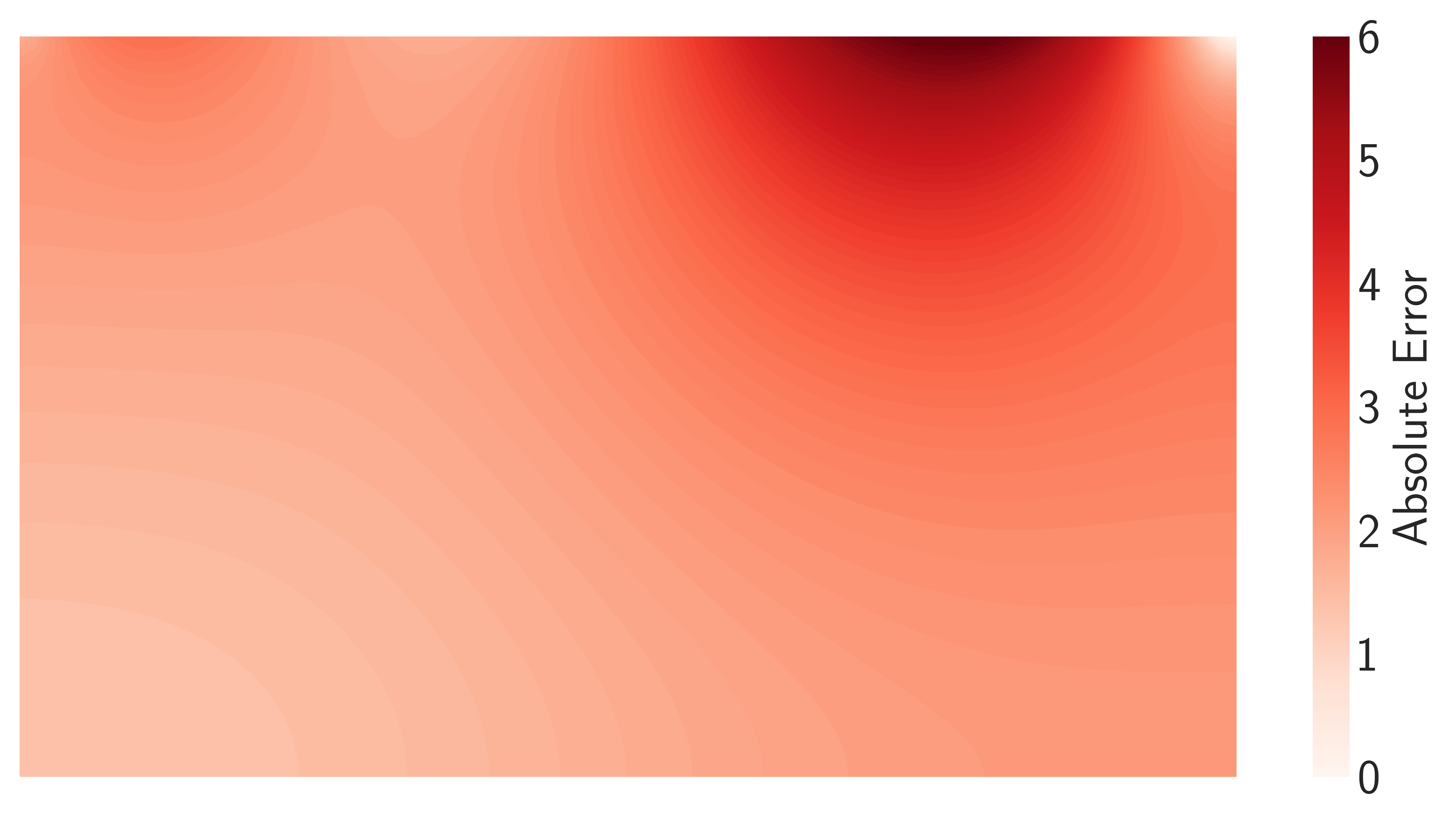
(b)

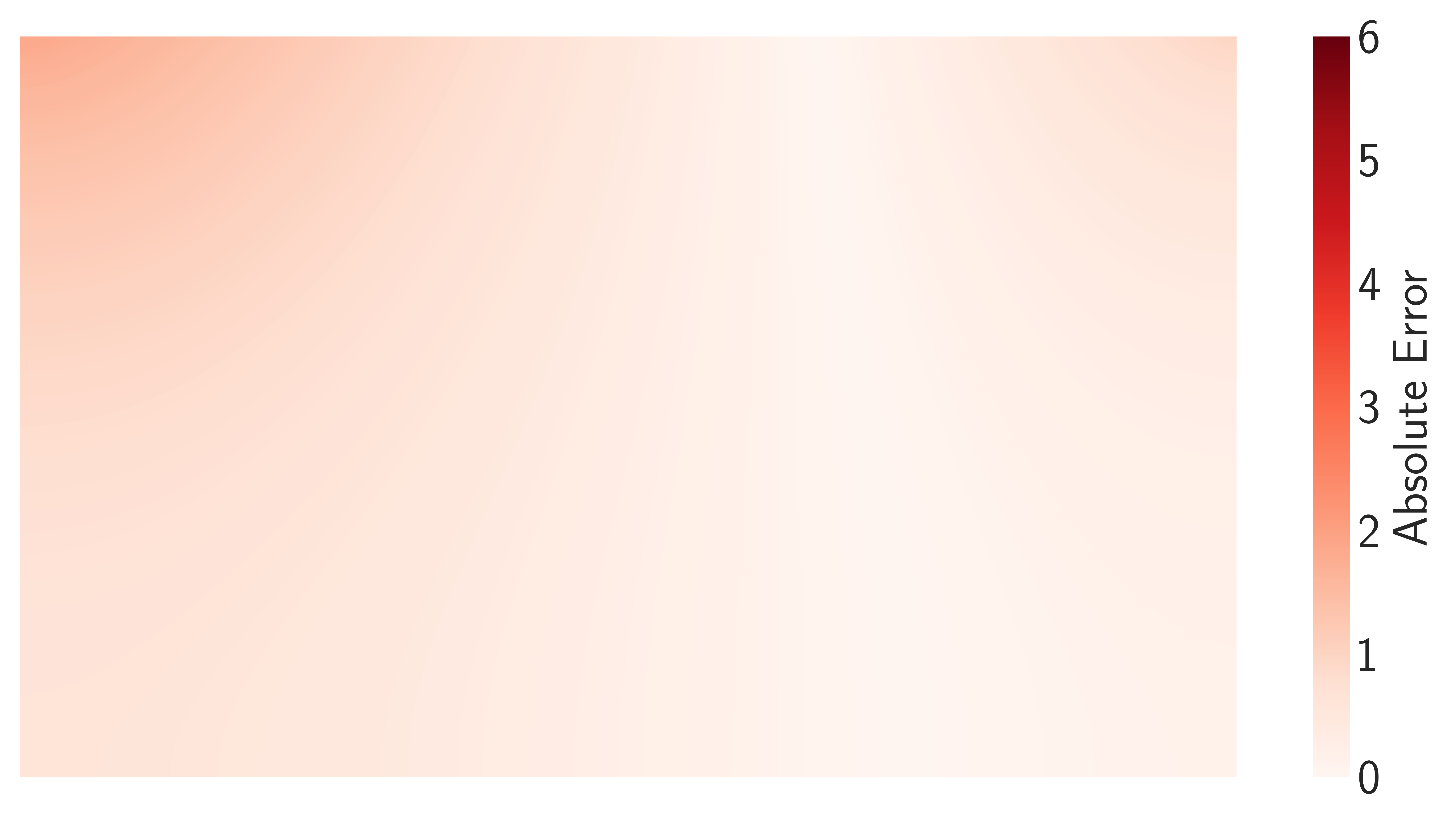
(c)

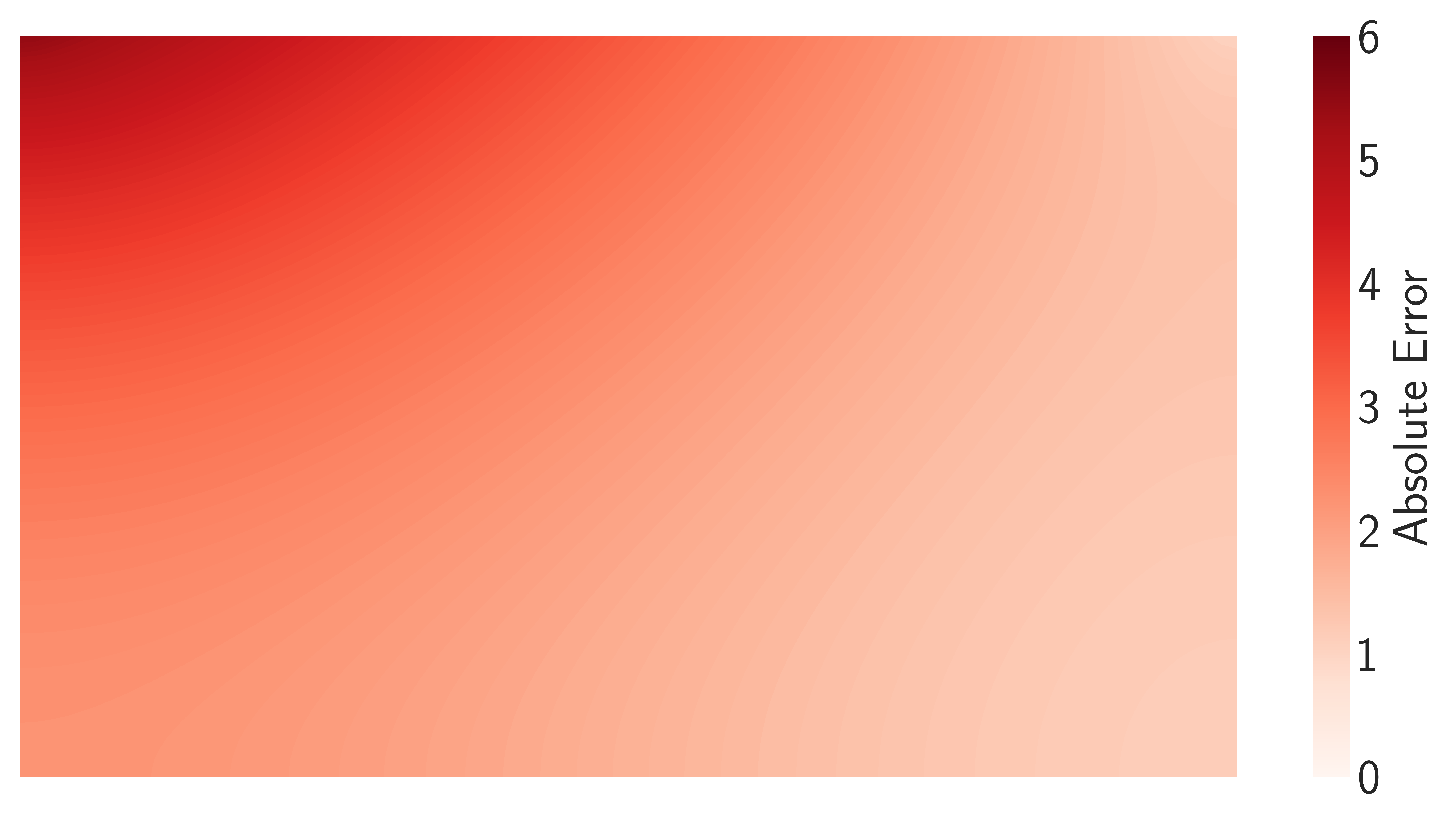
(d)

Figure 19: Absolute error between the true scalar field and the scalar field obtained by the average optimized design vectors presented in Fig. 17 for both BC cases: (a) True and $PSO_{ML-EN}$ scalar field absolute error for the sinusoidal BC (b) True and PSO scalar field absolute error for the sinusoidal BC (c) True and $PSO_{ML-EN}$ scalar field absolute error for the linear BC (d) True and PSO scalarfield absolute error for the linear BC.

6.4 Advantages and Limitations of the ML-enhanced Framework

While the ML-enhanced inverse design method shows improved performance, it is not without limitations. Primarily, the framework requires a pre-trained ML model to estimate the M_info value. To harness this model effectively for search space reduction and to cut back on the number of HF simulations, it is vital to understand and determine the pertinent reduced-order information related to the optimization challenge.

The main advantage of the proposed method is that an ML model is trained independently of the optimization loop using LF data only, and can then be exploited for different inverse design instances of the same type of problem (e.g., one ML model for airfoils enables the efficient optimization of multiple different types of airfoils). Furthermore, the ML model does not have to be highly accurate as highlighted in the detailed hyperparameter analysis for both investigated problems, which is advantageous in cases where obtaining LF data is computationally non-trivial.

Another limitation of the framework lies in its dependence on multiple hyperparameters. Both the search space reduction technique, as applied to AID, and the ML-enhanced framework itself require safety hyperparameters ($\eta$ and $c$ respectively). Although this study demonstrates that the $c$ value can correlate with the $RMSE$ of the model suggesting values of $c\in\{0.5,1,2\}$ for both problem a more exhaustive analysis encompassing a broader set of similar problems is essential. However, pinpointing the appropriate $c$ parameter could be accomplished through an exploratory analysis leveraging an ML model and exclusively LF simulations.

7 Conclusion

The paper presents an ML-enhanced inverse design framework for problems with stringent simulation budgets. This framework, applied to two distinct engineering challenges–AID and SFR–leveraged a pre-trained ML model. The goal was to reduce the size of the optimization search space and to decrease the need for costly HF simulations to arrive at an optimal design. In this ML-enhanced framework, both the DE and PSO optimization algorithms, which have an extensive demand for objective function evaluations, were enhanced with the ML model and contrasted with their conventional versions.

The main contributions of the study can be summarized in several points:

• An ML model trained on a small set of LF data effectively reduces the optimization search space. This facilitates a better rate of convergence of both PSO and DE towards a better approximation of the target performance within a predefined HF simulation budget.

• The ML-framework proves highly effective for both minimizing the number of HF simulations and approximating user-defined target designs. A relationship between the ML model’s error metric ($RMSE$) and the mechanism for minimizing HF simulations has been established and explored. For the AID and SFR problems, the hyperparameter $c$ which is used to multiply the $RMSE$, is recommended to be in the range $c\in\{0.5,1,2\}$.

• The solutions obtained with population-based stochastic global optimization algorithms, such as DE and PSO, can be significantly improved when guided by ML models.

• The effectiveness of the ML-enhanced inverse design framework was demonstrated on two conceptually different engineering challenges.

For the AID problem, future studies could delve into the integration of sophisticated computational fluid dynamics models like the Reynolds-averaged Navier–Stokes (RANS) or LES as the main HF simulators in the optimization loop, complemented by the ML model. Regarding the SFR problem, research emphasis should be on increasing the problem complexity, e.g., by employing a fully transient simulation model, integrating the diffusion coefficient value into both the ML model and inverse design, and potentially utilizing the RANS model for flow field reconstruction [5]. Furthermore, an analysis of the influence of the number of field measurements should be conducted.

Generally, the ML-enhanced framework proposed here could find application in any problem where meaningful reduced-order information can be obtained and approximated using an ML model. Multiple scientific applications fall into this problem category including simulations in climate and combustion that can be run with different grid resolutions and time step sizes. The proposed framework could be implemented within a larger hybrid metaheuristic-Bayesian optimization framework to further minimize the number of HF function evaluations, and it could be further investigated with other derivative-free optimization algorithms.

Acknowledgments

This work was supported by the Laboratory Directed Research and Development Program of Lawrence Berkeley National Laboratory under U.S. Department of Energy Contract No. DE-AC02-05CH11231. Müller’s time was supported under U.S. Department of Energy Contract No. DE-AC36-08GO28308. Funding for math developments was provided by U.S. Department of Energy Office of Science, Office of Advanced Scientific Computing Research, Scientific Discovery through Advanced Computing (SciDAC) program through the FASTMath Institute. Funding for analysis of applications was provided by the Laboratory Directed Research and Development Program of the National Renewable Energy Laboratory.

Declarations

The authors have no relevant financial or non-financial interests to disclose.

Data availability

The data needed to reproduce the study is available upon reasonable request.

Appendix A Scalar Field Domain Probe Locations

In this section, the scalar measurement locations within the domain $\Omega$, used as postprocessing points for each OpenFOAM simulation, are presented. For the achievement of the target performance (scalar distribution) in both BC scenarios and for the training of ML models, the probe locations depicted in Fig. 20 and listed in Table 9 are to be used.

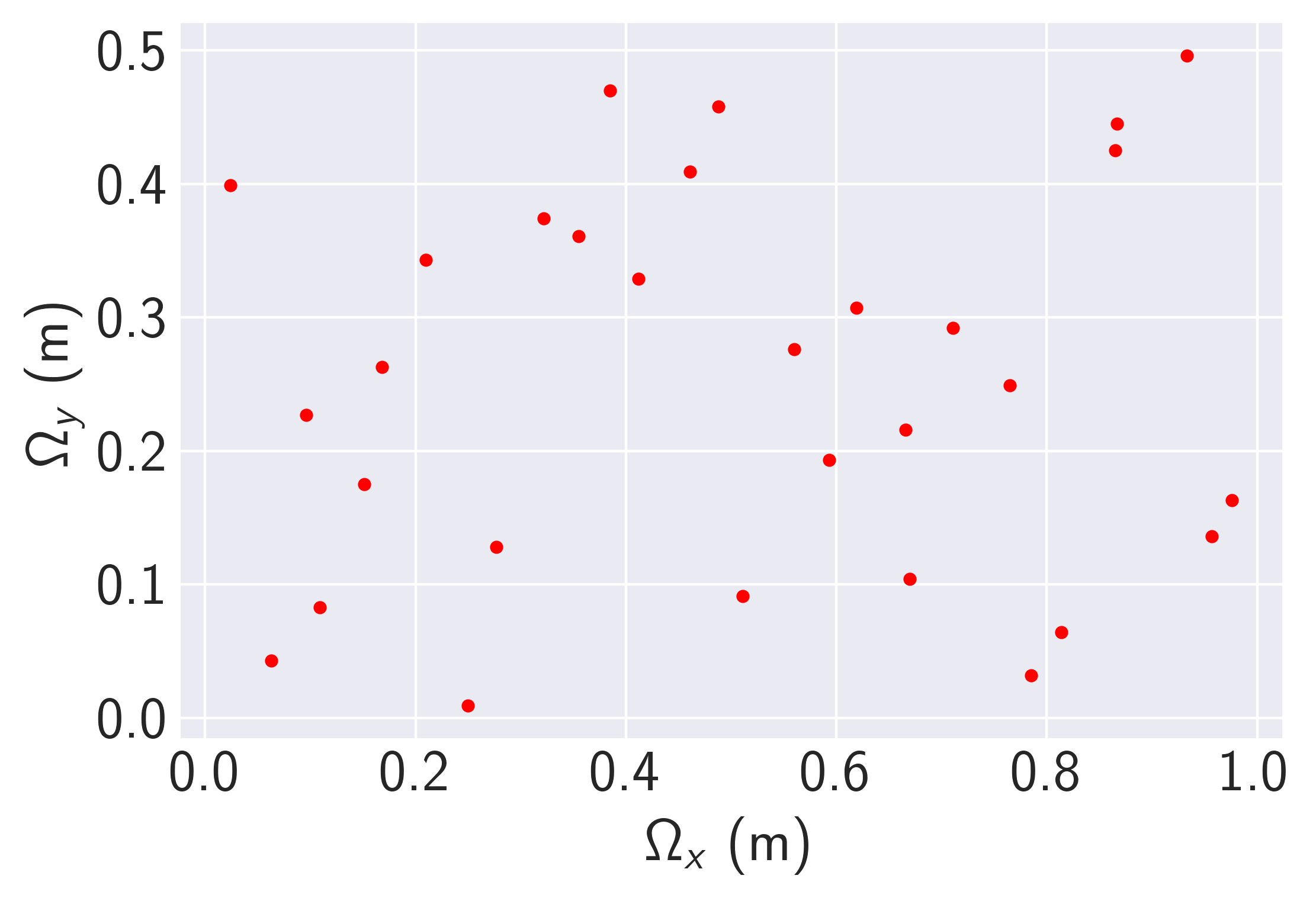
Figure 20: Scalar field reconstruction problem domain $\Omega$ with probe locations marked as red points. The boundary condition values are given at the top of the domain ($\Omega_{y}$ = 0.5 m).

Table 9: $\Omega_{x}$-axis and $\Omega_{y}$-axis values for all probe locations within the domain $\Omega$ for the scalar field reconstruction problem.

Probe	$\Omega_{x}$	$\Omega_{x}$
1	0.168	0.263
2	0.063	0.043
3	0.867	0.445
4	0.711	0.292
5	0.412	0.329
6	0.593	0.193
7	0.096	0.227
8	0.670	0.104
9	0.814	0.064
10	0.109	0.083
11	0.666	0.216
12	0.024	0.399
13	0.560	0.276
14	0.322	0.374
15	0.250	0.009
16	0.210	0.343
17	0.277	0.128
18	0.957	0.136
19	0.933	0.496
20	0.151	0.175
21	0.461	0.409
22	0.385	0.470
23	0.785	0.032
24	0.511	0.091
25	0.488	0.458
26	0.619	0.307
27	0.355	0.361
28	0.865	0.425
29	0.976	0.163
30	0.765	0.249

Appendix B Scalar Boundary Condition Generator

Fig. 21 illustrates the method used to generate the BC for scalar field reconstruction. The method begins with the values $LF_{n}$ and $s_{\Omega_{top}}$, which represent the number of LF discretization points at the top of the boundary and maximum scalar value that can be set a the top of the domain $\Omega$, respectively. The vector $\mathbf{BC}_{init}$ represents the initial BC. It consists of points that are equally spaced and sized $LF_{n}$. These points are derived from linear interpolation of values ranging from 1 to $LF_{n}$. A value $R$ is randomly chosen from a uniform distribution, representing one of three states that signify different BC variations: linear, parabolic, or sinusoidal. $\mathbf{G}_{noise}$ is a random vector, generated from a normal distribution, with a length of $LF_{n}$. Its standard deviation, $\sigma$, is drawn from a uniform distribution. This vector is added to the transformed $\mathbf{BC}$ to enhance model robustness, simulate real-world scenarios, and ensure better generalization in imperfect or noisy environments.

For each run, one of the three BC types is chosen and $\mathbf{BC}_{init}$ is transformed using the corresponding equation (linear, parabolic, or sinusoidal) incorporating randomly generated values $rand_{1}$, $rand_{2}$, and $rand_{3}$ from a uniform distribution. If the resultant $\mathbf{BC}$ with added noise $\mathbf{G}_{noise}$ has values exceeding $s_{max}$, they are substituted with a random value between 0 and $s_{max}$. To further diversify the generated BCs, if a random value between 0 and 1 is less than 0.5, the $\mathbf{BC}$ is reversed.

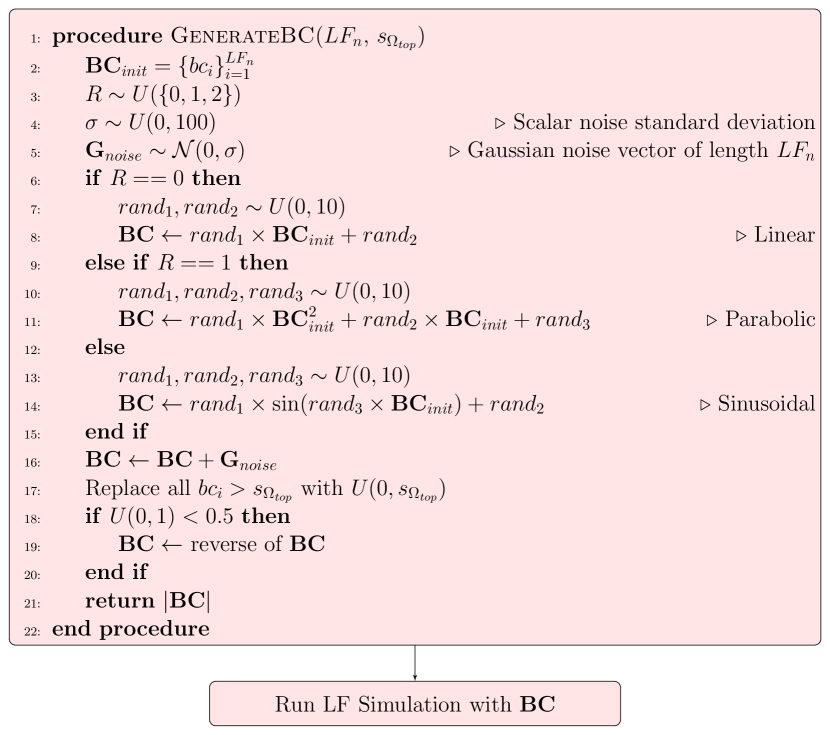
Figure 21: The procedure for generating the scalar reconstruction problem BC for the purpose of ML model training dataset creation.

Appendix C Search Space Reduction Convergence

Fig. 22 illustrates the impact of both the dataset size used for training the XGB model and the number of solutions, $N$, derived from the search space reduction technique on the formation of the new lower and upper boundaries, $\mathbf{lb}_{R}$ and $\mathbf{ub}_{R}$, respectively. Since these new boundaries can be interpreted as an airfoil shape, the effect of the dataset size and the $N$ value is articulated through the average and standard deviation of the $\zeta_{y}$ values (the chord length-normalized y-coordinates of the airfoil defined by $\mathbf{lb}_{R}$ and $\mathbf{ub}_{R}$).

For 10, 50, and 150 runs (or solutions), the average $\zeta_{y}$ and its standard deviation bandwidth exhibit only minor variations as the dataset size increases. This trend is discernible for both $NACA2410$ and $RAE2822$ in Fig. 22(a) and Fig. 22(b). This implies that even a search space reduction formulated by an XGB model trained with just 500 data instances and merely 10 repeated runs could be beneficial, as the boundaries remain relatively consistent despite increases in both parameters.

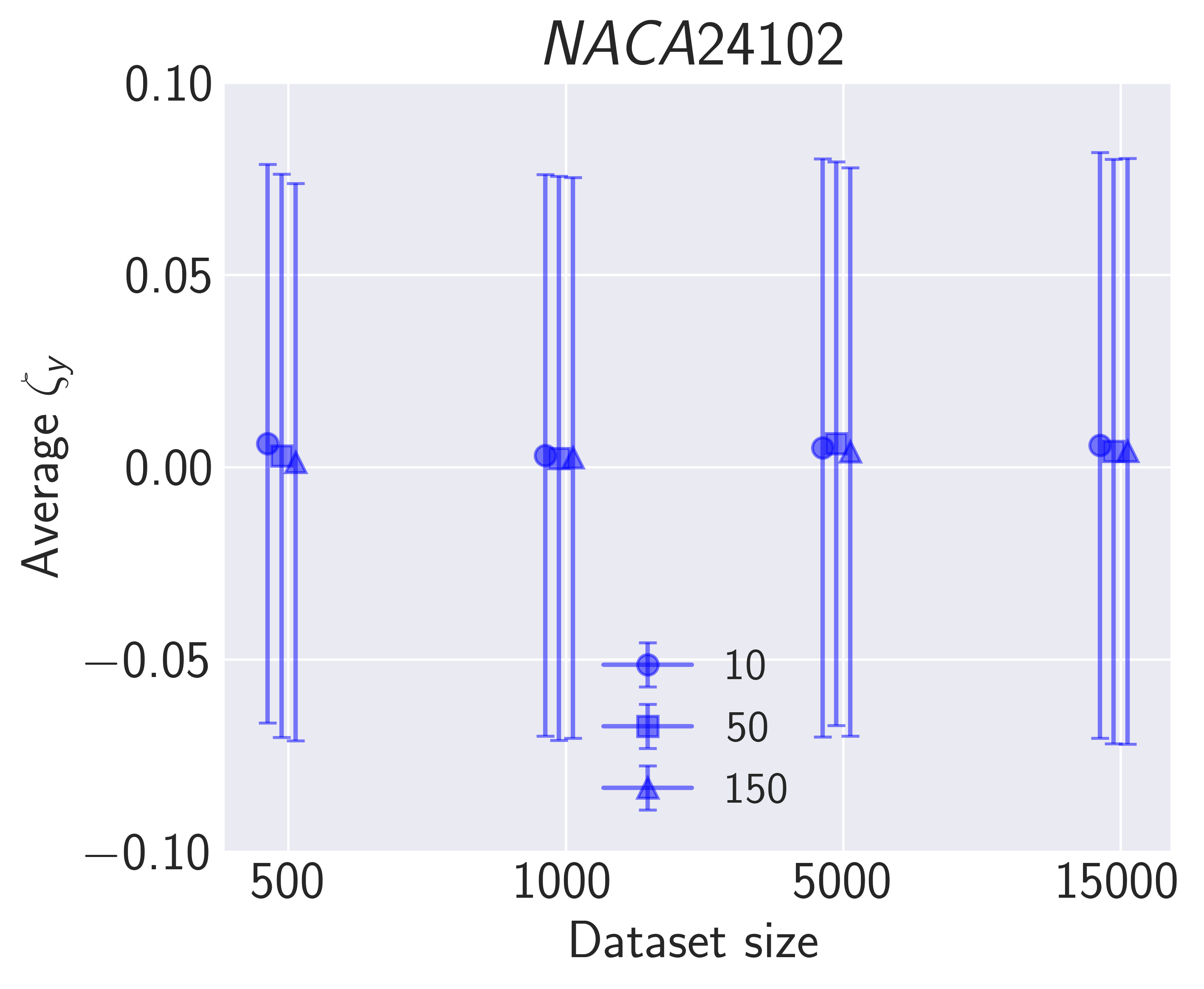
(a)

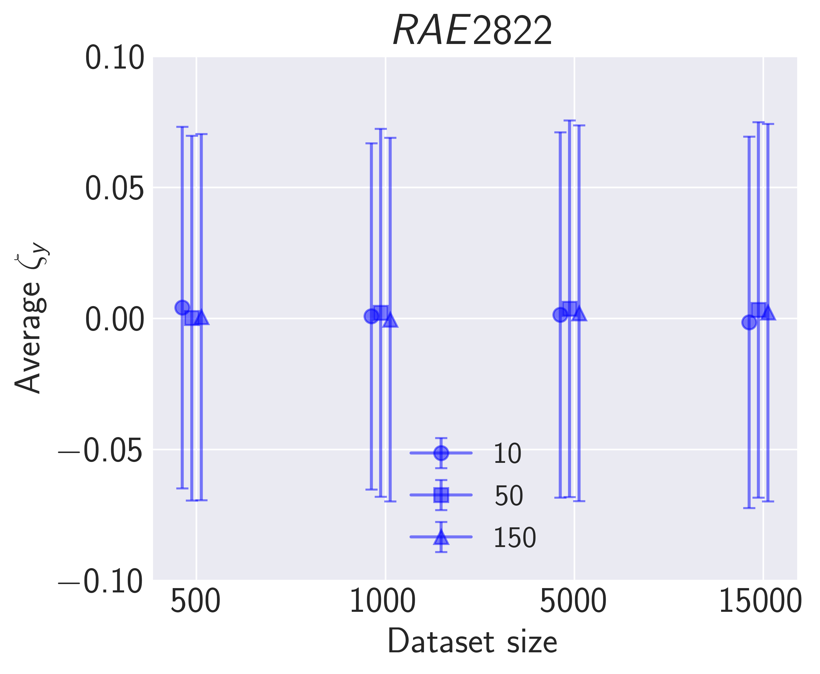
(b)

Figure 22: Search space reduction technique for different datasets sizes used to train the XGB model versus the average $\zeta_{y}$ for (a) $NACA2410$ airfoil and (b) $RAE2822$ airfoil. The number of solutions $N$ (denoted as runs) was varied to analyze how it affects the average $\zeta_{y}$. The markers are slightly offset for each $c$ value to improve visibility.

Fig. 23 demonstrates the impact of the number of solutions, $N$, and the dataset size on the average scalar value $\overline{s}$ of the BC. Mirroring observations from the AID search space reduction, neither the dataset size nor the number of solutions exert a significant effect on $\overline{s}$.

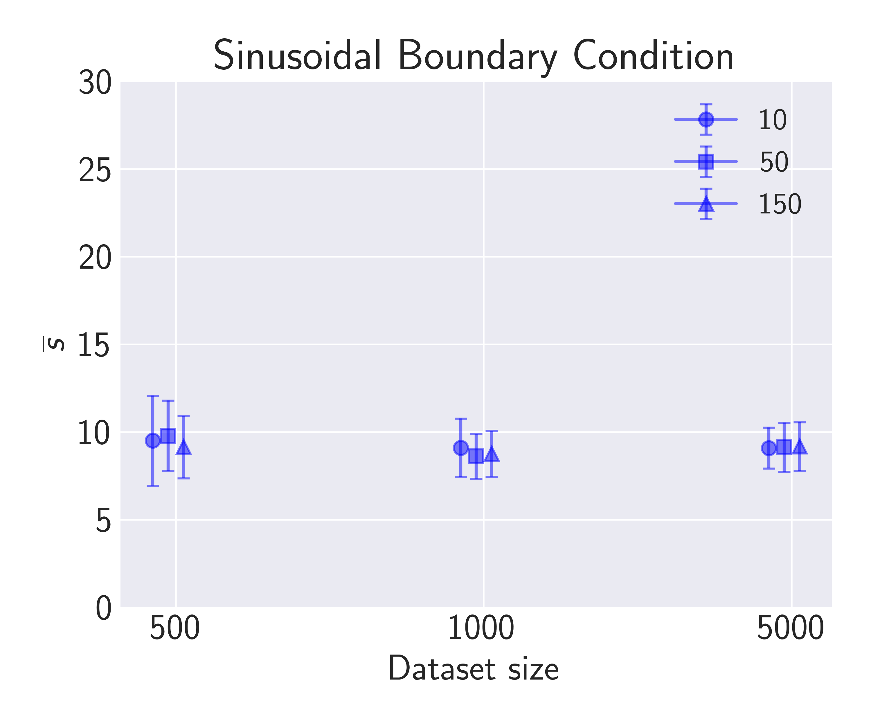
(a)

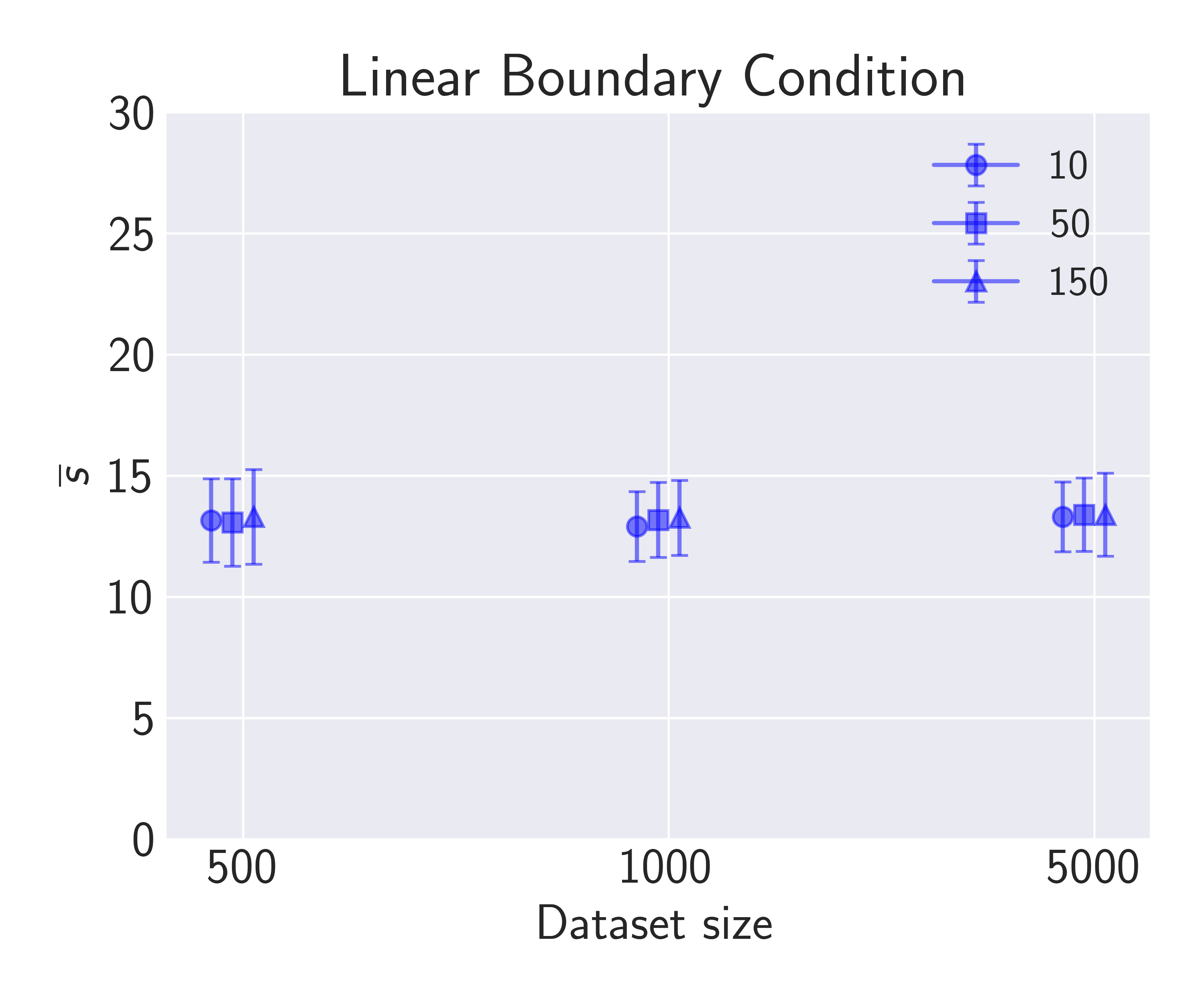
(b)

Figure 23: Search space reduction technique for different datasets sizes used to train the MLP model versus the average scalar value of the BC $\overline{s}$ for the (a) Sinusoidal BC and (b) Linear BC. The number of solutions $N$ (denoted as runs) was varied to observe its influence on the average $s$ value. The markers are slightly offset for each $c$ value to improve visibility.

Appendix D AID Results for $\eta$ = 1.1 and $\eta$ = 1.2

The results of the ML-enhanced inverse design framework utilizing the XGB model and the search space reduction technique ($\eta$ = 1.1 and $\eta$ = 1.2) applied to the AID problem for the $NACA2410$ and $RAE2822$ airfoils are shown in Figures 24 and 25.

(a)

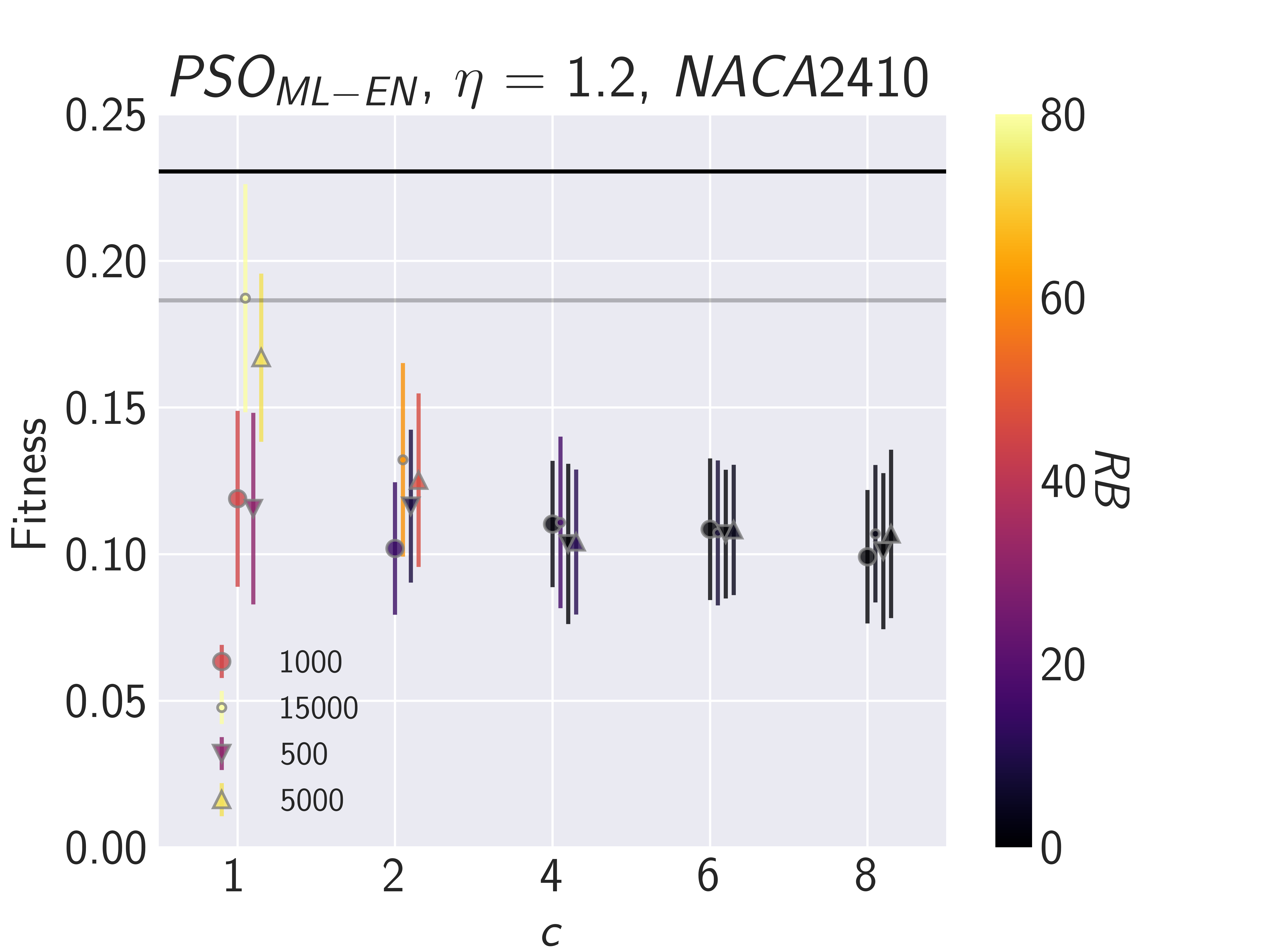
(b)

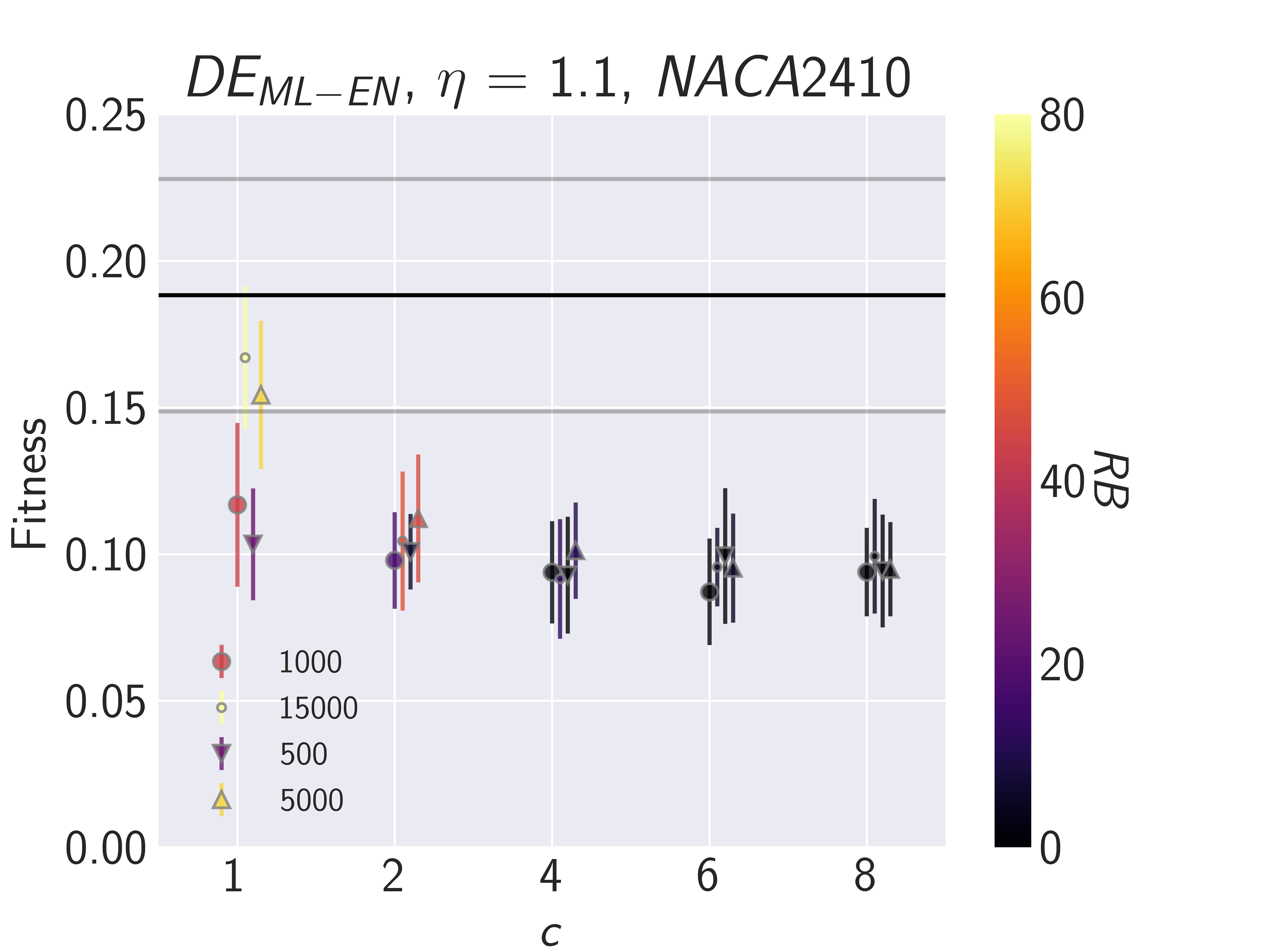
(c)

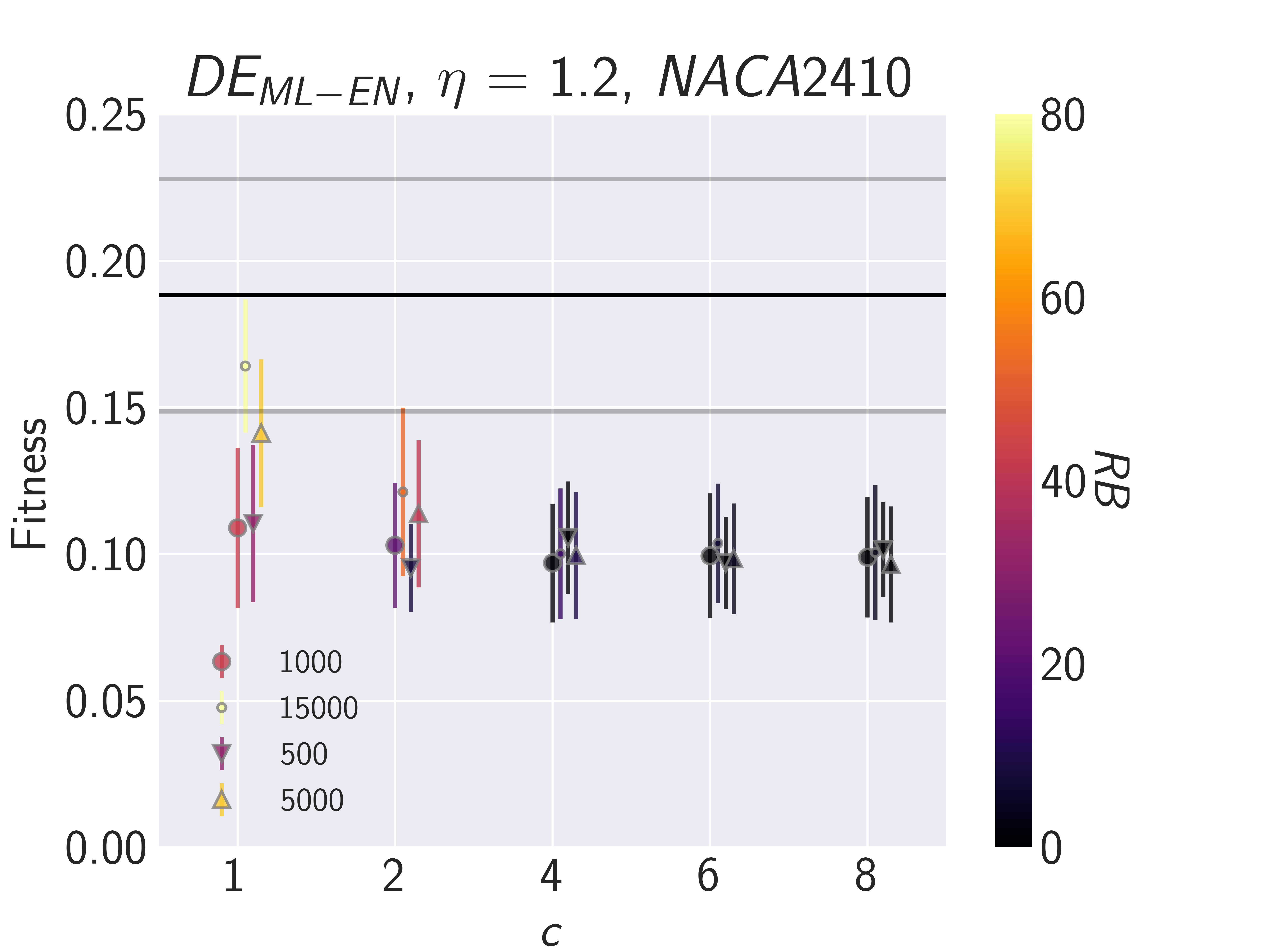
(d)

Figure 24: Results from the ML-enhanced framework for NACA2410 include the following search space reduction configurations: (a) $PSO_{ML-EN}$, $\eta$ = 1.1 (b) $PSO_{ML-EN}$, $\eta$ = 1.2 (c) $DE_{ML-EN}$, $\eta$ = 1.1 (d) $DE_{ML-EN}$, $\eta$ = 1.2. The markers denote the different dataset sizes used to train the ML model, while the coloring of the markers represents the remaining simulation budget ($RB$) values. A higher $RB$ signifies greater savings in the computational budget, while low fitness values imply a better approximation of the target performance. The markers are slightly offset for each $c$ value to improve visibility.

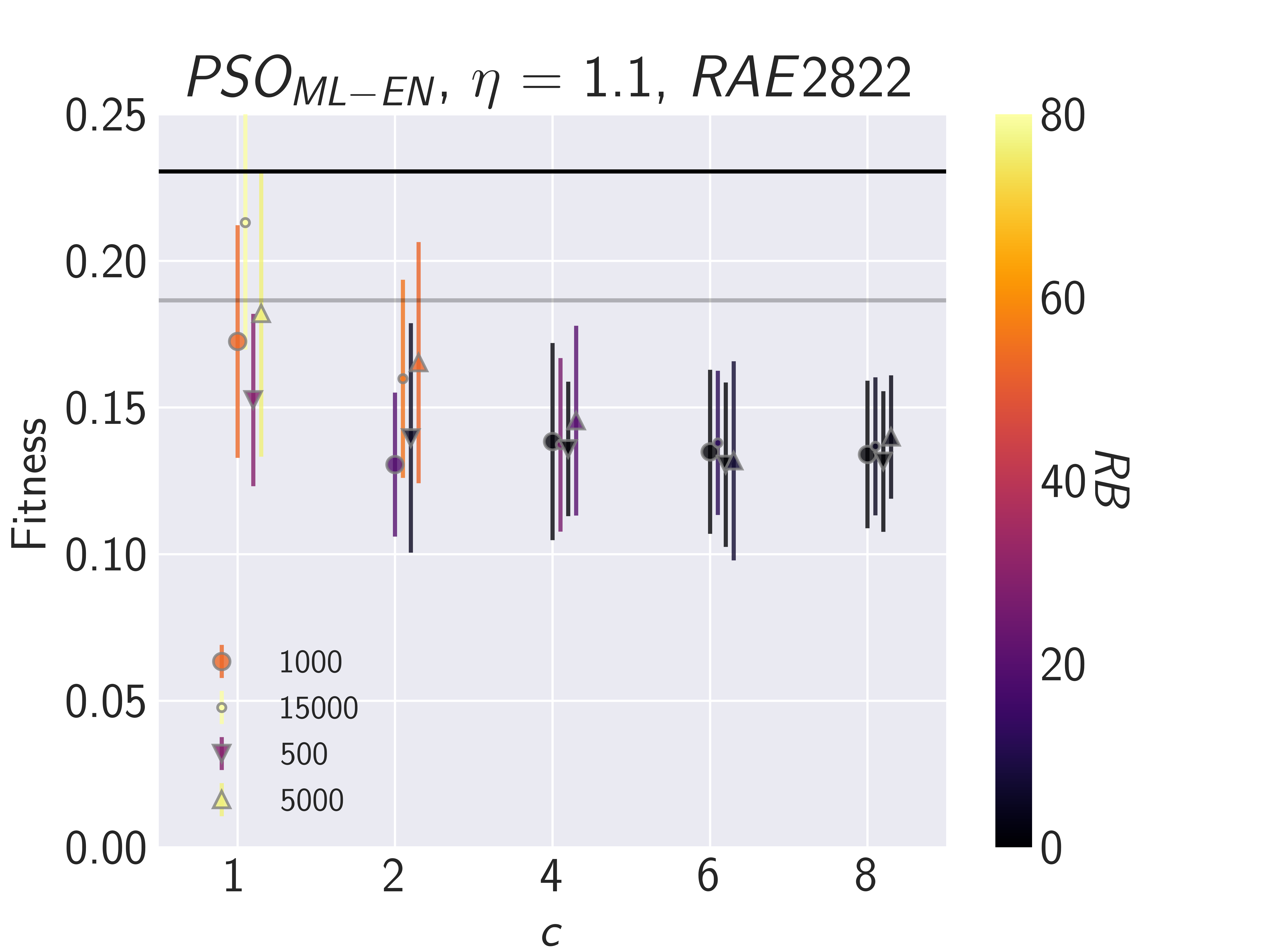
(a)

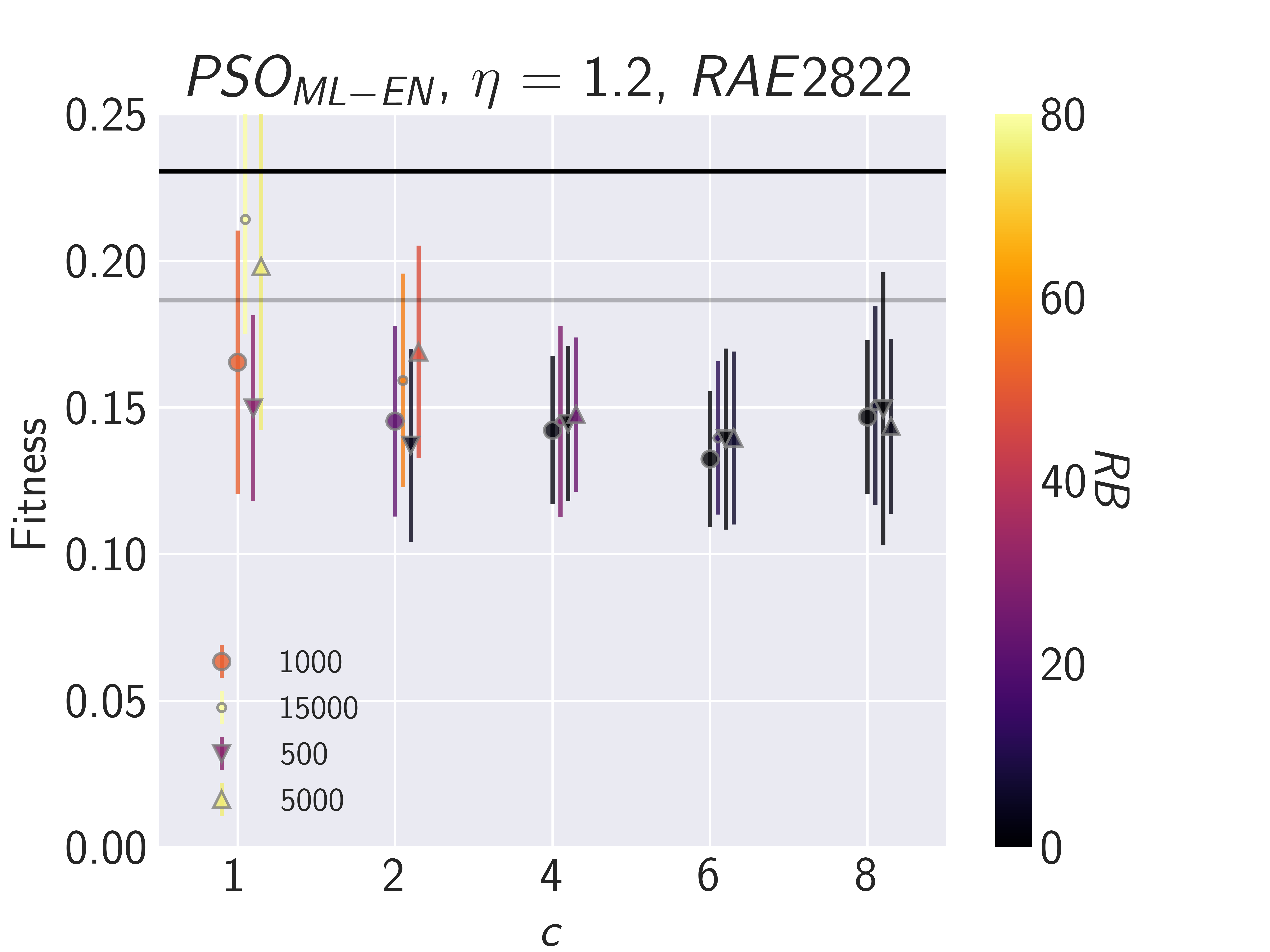
(b)

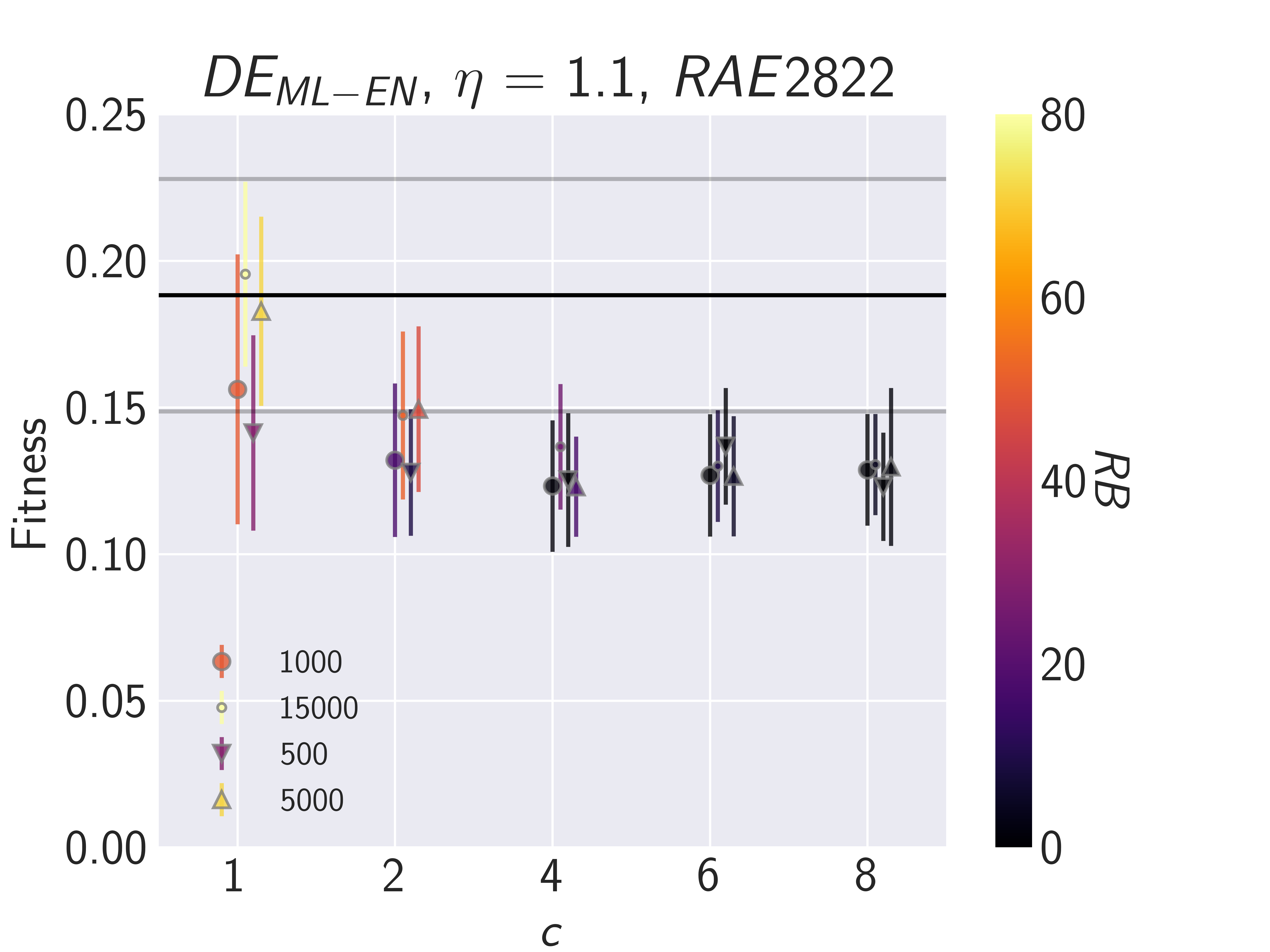
(c)

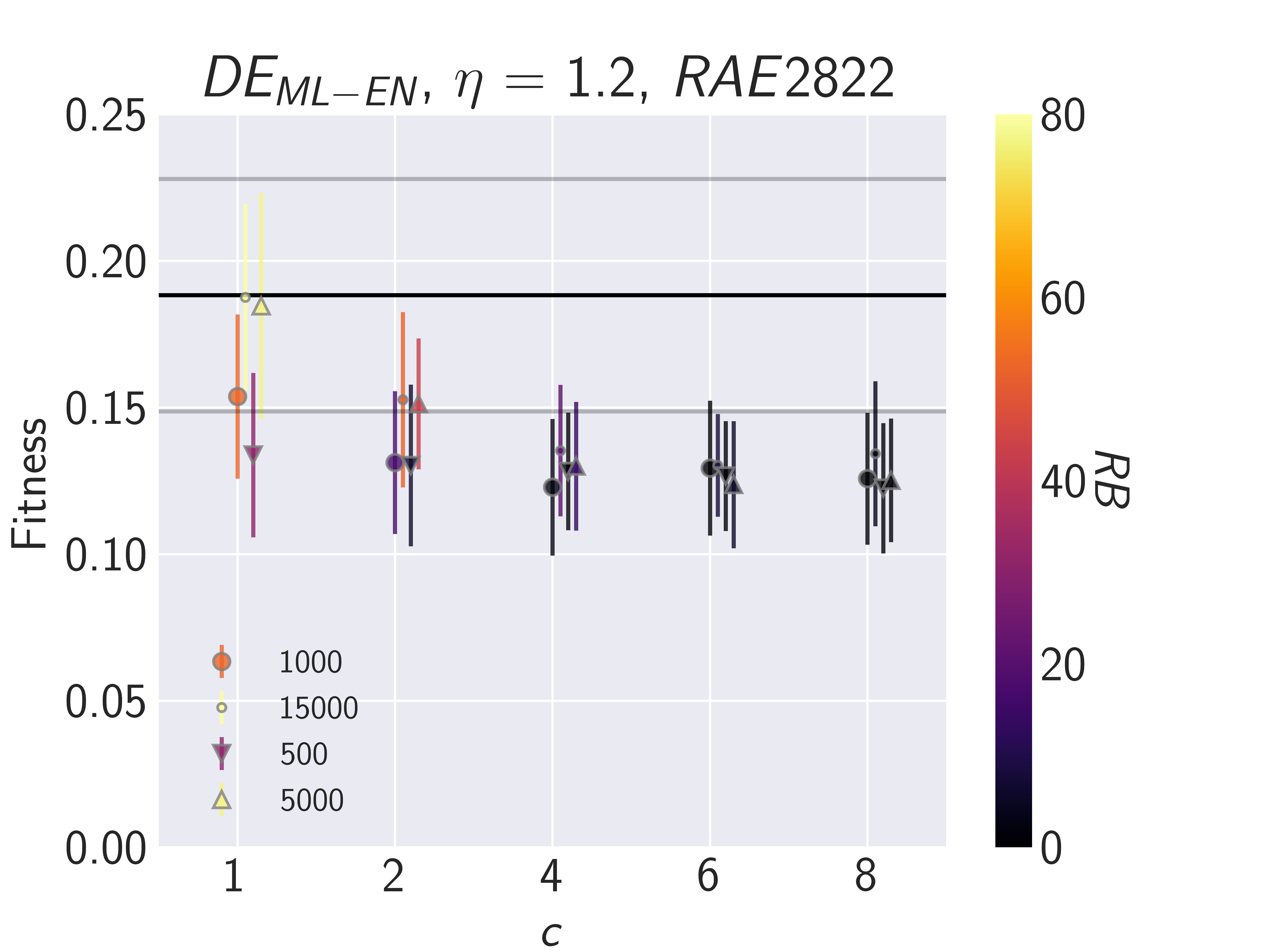
(d)

Figure 25: Results from the ML-enhanced framework for $RAE2822$ include the following search space reduction configurations: (a) $PSO_{ML-EN}$, $\eta$ = 1.1 (b) $PSO_{ML-EN}$, $\eta$ = 1.2 (c) $DE_{ML-EN}$, $\eta$ = 1.1 (d) $DE_{ML-EN}$, $\eta$ = 1.2. The markers denote the different dataset sizes used to train the ML model, while the coloring of the markers represents the remaining simulation budget ($RB$) values. A higher $RB$ signifies greater savings in the computational budget, while low fitness values imply a better approximation of the target performance. The markers are slightly offset for each $c$ value to improve visibility.

References

- \bibcommenthead
- Abadi et al [2016] Abadi M, Agarwal A, Barham P, et al (2016) Tensorflow: Large-scale machine learning on heterogeneous distributed systems. arXiv preprint arXiv:160304467 https://doi.org/10.48550/arXiv.1603.04467
- Akiba et al [2019] Akiba T, Sano S, Yanase T, et al (2019) Optuna: A next-generation hyperparameter optimization framework. In: Proceedings of the 25th ACM SIGKDD international conference on knowledge discovery & data mining, pp 2623–2631, https://doi.org/10.1145/3292500.3330701
- Aster et al [2018] Aster RC, Borchers B, Thurber CH (2018) Parameter estimation and inverse problems. Elsevier
- Bartoli et al [2019] Bartoli N, Lefebvre T, Dubreuil S, et al (2019) Adaptive modeling strategy for constrained global optimization with application to aerodynamic wing design. Aerospace Science and technology 90:85–102. https://doi.org/10.1016/j.ast.2019.03.041
- Brunton et al [2020] Brunton SL, Noack BR, Koumoutsakos P (2020) Machine learning for fluid mechanics. Annual review of fluid mechanics 52:477–508. https://doi.org/10.1146/annurev-fluid-010719-060214
- Chen and Zhou [2018] Chen H, Zhou H (2018) Identification of boundary conditions for non-fourier heat conduction problems by differential transformation drbem and improved cuckoo search algorithm. Numerical Heat Transfer, Part B: Fundamentals 74(6):818–839. https://doi.org/10.1080/10407790.2019.1591859
- Chen et al [2018] Chen Hl, Yu B, Zhou Hl, et al (2018) Identification of transient boundary conditions with improved cuckoo search algorithm and polynomial approximation. Engineering Analysis with Boundary Elements 95:124–141. https://doi.org/10.1016/j.enganabound.2018.07.006
- Chen and Guestrin [2016] Chen T, Guestrin C (2016) Xgboost: A scalable tree boosting system. In: Proceedings of the 22nd acm sigkdd international conference on knowledge discovery and data mining, pp 785–794, https://doi.org/10.1145/2939672.2939785
- Chen et al [2022] Chen Z, Wang P, Bao S, et al (2022) Rapid reconstruction of temperature and salinity fields based on machine learning and the assimilation application. Frontiers in Marine Science 9:985048. https://doi.org/10.3389/fmars.2022.985048
- Deng and Yi [2023] Deng F, Yi J (2023) Fast inverse design of transonic airfoils by combining deep learning and efficient global optimization. Aerospace 10(2):125. https://doi.org/10.3390/aerospace10020125
- Drela [1989] Drela M (1989) Xfoil: An analysis and design system for low reynolds number airfoils. In: Low Reynolds Number Aerodynamics: Proceedings of the Conference Notre Dame, Indiana, USA, 5–7 June 1989, Springer, pp 1–12
- Du et al [2019] Du X, Ren J, Leifsson L (2019) Aerodynamic inverse design using multifidelity models and manifold mapping. Aerospace Science and Technology 85:371–385. https://doi.org/10.1016/j.ast.2018.12.008
- Du et al [2021] Du X, He P, Martins JR (2021) Rapid airfoil design optimization via neural networks-based parameterization and surrogate modeling. Aerospace Science and Technology 113:106701. https://doi.org/10.1016/j.ast.2021.106701
- Eldred and Dunlavy [2006] Eldred M, Dunlavy D (2006) Formulations for surrogate-based optimization with data fit, multifidelity, and reduced-order models. In: 11th AIAA/ISSMO multidisciplinary analysis and optimization conference, p 7117, https://doi.org/10.2514/6.2006-7117
- Forrester et al [2008] Forrester A, Sobester A, Keane A (2008) Engineering design via surrogate modelling: a practical guide. John Wiley & Sons, https://doi.org/10.1002/9780470770801
- Gong et al [2023] Gong Z, Zhou W, Zhang J, et al (2023) Joint deep reversible regression model and physics-informed unsupervised learning for temperature field reconstruction. Engineering Applications of Artificial Intelligence 118:105686. https://doi.org/10.1016/j.engappai.2022.105686
- Gordillo et al [2020] Gordillo G, Morales-Hernández M, García-Navarro P (2020) A gradient-descent adjoint method for the reconstruction of boundary conditions in a river flow nitrification model. Environmental Science: Processes & Impacts 22(2):381–397. https://doi.org/10.1039/C9EM00500E
- Han et al [2013] Han ZH, Görtz S, Zimmermann R (2013) Improving variable-fidelity surrogate modeling via gradient-enhanced kriging and a generalized hybrid bridge function. Aerospace Science and technology 25(1):177–189. https://doi.org/10.1016/j.ast.2012.01.006
- Han et al [2018] Han ZH, Chen J, Zhang KS, et al (2018) Aerodynamic shape optimization of natural-laminar-flow wing using surrogate-based approach. AIAA Journal 56(7):2579–2593. https://doi.org/10.2514/1.J056661
- Hanna et al [2005] Hanna S, Russell A, Wilkinson J, et al (2005) Monte carlo estimation of uncertainties in beis3 emission outputs and their effects on uncertainties in chemical transport model predictions. Journal of Geophysical Research: Atmospheres 110(D1). https://doi.org/10.1029/2004JD004986
- He et al [2023] He C, Zhang Y, Gong D, et al (2023) A review of surrogate-assisted evolutionary algorithms for expensive optimization problems. Expert Systems with Applications p 119495. https://doi.org/10.1016/j.eswa.2022.119495
- Huang et al [2022] Huang Z, Li T, Huang K, et al (2022) Predictions of flow and temperature fields in a t-junction based on dynamic mode decomposition and deep learning. Energy 261:125228. https://doi.org/10.1016/j.energy.2022.125228
- Ivic et al [2023] Ivic S, Druzeta S, Grbcic L (2023) Indago 0.4.5. PyPI, URL https://pypi.org/project/Indago/, accessed: 1 May 2023
- Jaluria [2020] Jaluria Y (2020) Solution of inverse problems in thermal systems. Journal of Thermal Science and Engineering Applications 12(1):011005. https://doi.org/10.1115/1.4042353
- Jasak et al [2007] Jasak H, Jemcov A, Tukovic Z, et al (2007) Openfoam: A c++ library for complex physics simulations. In: International workshop on coupled methods in numerical dynamics, pp 1–20
- Karr et al [2000] Karr CL, Yakushin I, Nicolosi K (2000) Solving inverse initial-value, boundary-value problems via genetic algorithm. Engineering Applications of Artificial Intelligence 13(6):625–633. https://doi.org/10.1016/S0952-1976(00)00025-7
- Ke et al [2017] Ke G, Meng Q, Finley T, et al (2017) Lightgbm: A highly efficient gradient boosting decision tree. Advances in neural information processing systems 30
- Kennedy and Eberhart [1995] Kennedy J, Eberhart R (1995) Particle swarm optimization. In: Proceedings of ICNN’95-international conference on neural networks, IEEE, pp 1942–1948, https://doi.org/10.1109/ICNN.1995.488968
- Koziel and Leifsson [2013] Koziel S, Leifsson L (2013) Surrogate-based aerodynamic shape optimization by variable-resolution models. AIAA journal 51(1):94–106. https://doi.org/10.2514/1.J051583
- Lei et al [2021] Lei R, Bai J, Wang H, et al (2021) Deep learning based multistage method for inverse design of supercritical airfoil. Aerospace Science and Technology 119:107101. https://doi.org/10.1016/j.ast.2021.107101
- Leifsson et al [2011] Leifsson L, Koziel S, Ogurtsov S (2011) Inverse design of transonic airfoils using variable-resolution modeling and pressure distribution alignment. Procedia Computer Science 4:1234–1243. https://doi.org/10.1016/j.procs.2011.04.133
- Li et al [2022] Li J, Du X, Martins JR (2022) Machine learning in aerodynamic shape optimization. Progress in Aerospace Sciences 134:100849. https://doi.org/10.1016/j.paerosci.2022.100849
- Li et al [2023] Li J, He S, Martins JR, et al (2023) Efficient data-driven off-design constraint modeling for practical aerodynamic shape optimization. AIAA Journal pp 1–13. https://doi.org/10.2514/1.J062629
- Liu et al [2020] Liu T, Li Y, Xie Y, et al (2020) Deep learning for nanofluid field reconstruction in experimental analysis. Ieee Access 8:64692–64706. https://doi.org/10.1109/ACCESS.2020.2979794
- Liu et al [2021] Liu T, Li Y, Jing Q, et al (2021) Supervised learning method for the physical field reconstruction in a nanofluid heat transfer problem. International Journal of Heat and Mass Transfer 165:120684. https://doi.org/10.1016/j.ijheatmasstransfer.2020.120684
- Ma et al [2019] Ma T, Liu Y, Cao C (2019) Neural networks for 3d temperature field reconstruction via acoustic signals. Mechanical systems and signal processing 126:392–406. https://doi.org/10.1016/j.ymssp.2019.02.037
- Marzouk and Xiu [2009] Marzouk Y, Xiu D (2009) A stochastic collocation approach to bayesian inference in inverse problems. Communications in Computational Physics 6(4):826–847
- Mohasseb et al [2017] Mohasseb S, Moradi M, Sokhansefat T, et al (2017) A novel approach to solve inverse heat conduction problems: Coupling scaled boundary finite element method to a hybrid optimization algorithm. Engineering Analysis with Boundary Elements 84:206–212. https://doi.org/10.1016/j.enganabound.2017.08.018
- Morgado et al [2016] Morgado J, Vizinho R, Silvestre M, et al (2016) Xfoil vs cfd performance predictions for high lift low reynolds number airfoils. Aerospace Science and Technology 52:207–214. https://doi.org/10.1016/j.ast.2016.02.031
- Nielsen [2015] Nielsen MA (2015) Neural networks and deep learning, vol 25. Determination press San Francisco, CA, USA
- Peherstorfer et al [2018] Peherstorfer B, Willcox K, Gunzburger M (2018) Survey of multifidelity methods in uncertainty propagation, inference, and optimization. Siam Review 60(3):550–591. https://doi.org/10.1137/16M1082469
- Pehlivanoglu [2019] Pehlivanoglu YV (2019) Efficient accelerators for pso in an inverse design of multi-element airfoils. Aerospace Science and Technology 91:110–121. https://doi.org/10.1016/j.ast.2019.05.028
- Qiu et al [2016] Qiu H, Xu Y, Gao L, et al (2016) Multi-stage design space reduction and metamodeling optimization method based on self-organizing maps and fuzzy clustering. Expert Systems with Applications 46:180–195. https://doi.org/10.1016/j.eswa.2015.10.033
- Rajnarayan et al [2018] Rajnarayan D, Ning A, Mehr JA (2018) Universal airfoil parametrization using b-splines. In: 2018 Applied Aerodynamics Conference, p 3949, https://doi.org/10.2514/6.2018-3949
- Ren et al [2021] Ren T, Li H, Modest MF, et al (2021) Efficient two-dimensional scalar fields reconstruction of laminar flames from infrared hyperspectral measurements with a machine learning approach. Journal of Quantitative Spectroscopy and Radiative Transfer 271:107724. https://doi.org/10.1016/j.jqsrt.2021.107724
- Ren et al [2022] Ren T, Li H, Modest MF, et al (2022) Machine learning applied to the retrieval of three-dimensional scalar fields of laminar flames from hyperspectral measurements. Journal of Quantitative Spectroscopy and Radiative Transfer 279:108047. https://doi.org/10.1016/j.jqsrt.2021.108047
- Sarkar et al [2019] Sarkar S, Mondal S, Joly M, et al (2019) Multifidelity and multiscale bayesian framework for high-dimensional engineering design and calibration. Journal of Mechanical Design 141(12):121001. https://doi.org/10.1115/1.4044598
- Sharma et al [2021] Sharma P, Gupta B, Pandey M, et al (2021) Recent advancements in optimization methods for wind turbine airfoil design: A review. Materials Today: Proceedings 47:6556–6563. https://doi.org/10.1016/j.matpr.2021.02.231
- Słota [2008] Słota D (2008) Solving the inverse stefan design problem using genetic algorithms. Inverse Problems in Science and Engineering 16(7):829–846. https://doi.org/10.1080/17415970801925170
- Storn and Price [1997] Storn R, Price K (1997) Differential evolution–a simple and efficient heuristic for global optimization over continuous spaces. Journal of global optimization 11:341–359. https://doi.org/10.1023/A:1008202821328
- Tandis and Assareh [2017] Tandis E, Assareh E (2017) Inverse design of airfoils via an intelligent hybrid optimization technique. Engineering with Computers 33(3):361–374. https://doi.org/10.1007/s00366-016-0478-6
- Tarantola [2005] Tarantola A (2005) Inverse problem theory and methods for model parameter estimation. SIAM, https://doi.org/10.1137/1.9780898717921
- Virtanen et al [2020] Virtanen P, Gommers R, Oliphant TE, et al (2020) Scipy 1.0: fundamental algorithms for scientific computing in python. Nature methods 17(3):261–272. https://doi.org/10.1038/s41592-019-0686-2
- de Vries [2023] de Vries D (2023) xfoil-python 1.1.1. PyPI, URL https://pypi.org/project/xfoil/, accessed: 6 June 2023
- Wang et al [2022a] Wang C, Wang S, Wang L, et al (2022a) Framework of nacelle inverse design method based on improved generative adversarial networks. Aerospace Science and Technology 121:107365. https://doi.org/10.1016/j.ast.2022.107365
- Wang and Simpson [2004] Wang GG, Simpson T (2004) Fuzzy clustering based hierarchical metamodeling for design space reduction and optimization. Engineering Optimization 36(3):313–335. https://doi.org/10.1080/03052150310001639911
- Wang et al [2022b] Wang Z, Wang G, Guo X, et al (2022b) Reconstruction of high-resolution sea surface salinity over 2003–2020 in the south china sea using the machine learning algorithm lightgbm model. Remote Sensing 14(23):6147. https://doi.org/10.3390/rs14236147
- Winter et al [2023] Winter J, Abaidi R, Kaiser J, et al (2023) Multi-fidelity bayesian optimization to solve the inverse stefan problem. Computer Methods in Applied Mechanics and Engineering 410:115946. https://doi.org/10.1016/j.cma.2023.115946
- Xiao et al [2023] Xiao L, Chao S, Zhu Z, et al (2023) Three-dimensional aerodynamic shape inverse design based on isomap. Aerospace Science and Technology 139:108409. https://doi.org/10.1016/j.ast.2023.108409
- Xu et al [2016] Xu Y, Choi J, Dass S, et al (2016) Bayesian prediction and adaptive sampling algorithms for mobile sensor networks: Online environmental field reconstruction in space and time. Springer, https://doi.org/10.1007/978-3-319-21921-9
- Yang et al [2023] Yang S, Lee S, Yee K (2023) Inverse design optimization framework via a two-step deep learning approach: application to a wind turbine airfoil. Engineering with Computers 39(3):2239–2255. https://doi.org/10.1007/s00366-022-01617-6
- Yonekura et al [2022] Yonekura K, Miyamoto N, Suzuki K (2022) Inverse airfoil design method for generating varieties of smooth airfoils using conditional wgan-gp. Structural and Multidisciplinary Optimization 65(6):173. https://doi.org/10.1007/s00158-022-03253-6
- Zahir and Gao [2013] Zahir MK, Gao Z (2013) Variable-fidelity optimization with design space reduction. Chinese Journal of Aeronautics 26(4):841–849. https://doi.org/10.1016/j.cja.2013.06.002
- Zhang et al [2023] Zhang C, Duan Y, Chen H, et al (2023) Efficient aerodynamic shape optimization with the metric-based pod parameterization method. Structural and Multidisciplinary Optimization 66(6):140. https://doi.org/10.1007/s00158-023-03596-8
- Zhu et al [2020] Zhu Y, Ju Y, Zhang C (2020) Proper orthogonal decomposition assisted inverse design optimisation method for the compressor cascade airfoil. Aerospace Science and Technology 105:105955. https://doi.org/10.1016/j.ast.2020.105955