An Irredundant Decomposition of Data Flow with Affine Dependences

Abstract.

Optimization pipelines targeting polyhedral programs try to maximize the compute throughput. Traditional approaches favor reuse and temporal locality; while the communicated volume can be low, failure to optimize spatial locality may cause a low I/O performance.

Memory allocation schemes using data partitioning such as data tiling can improve the spatial locality, but they are domain-specific and rarely applied by compilers when an existing allocation is supplied.

In this paper, we propose to derive a partitioned memory allocation for tiled polyhedral programs using their data flow information. We extend the existing MARS partitioning (Ferry et al., 2023) to handle affine dependences, and determine which dependences can lead to a regular, simple control flow for communications.

While this paper consists in a theoretical study, previous work on data partitioning in inter-node scenarios has shown performance improvements due to better bandwidth utilization.

1. Introduction

The performance of programs is determined by multiple metrics, among which execution time and energy consumption. One of the main drivers of these two metrics is data movement: communication latency causes bottlenecks capping the compute throughput, and inter-chip communication significantly increases the power consumption. Optimizing data movement is a tedious task that involves significant modifications to the program; the extent of programs to optimize warrants automation. Powerful compiler analyses and abstractions have been developed in this aim, one of the most powerful of which is the polyhedral model.

In the polyhedral model, it is possible to entirely determine the execution sequence of a program, and its data movement. Optimizations are done in two respects: first, reducing the amount of communication by exhibiting locality; second, by optimizing the existing communications to reduce their latency and better utilize the available bandwidth.

Techniques improving bandwidth/access utilization (Bondhugula, 2013; Dathathri et al., 2013; Ferry et al., 2023) propose to decompose the data flowing between statements within a program and group together intermediate results based on their users; coalescing data accesses allows to better utilize the bandwidth. However, these data flow optimizations are too restrictive, because they omit all input data. Like it is done for intermediate results, input data transfers need to be optimized for both locality and memory access performance.

Furthermore, dependences to input variables are rarely uniform, because the data arrays usually have less dimensions than the domain of computation. The existing dependence-based partitioning works must therefore be extended to support affine dependences to input variables, and to propose a re-allocation of these variables.

This paper seeks to extend the partitioning of (Ferry et al., 2023) to handle the entire data flow of the tile and maximize access contiguity. Its contributions are as follows:

• We propose a partitioning scheme, called Affine-MARS, of data spaces and iteration spaces with a pre-existing tiling,

• We formalize the construction of this partitioning scheme and determine its limitations.

This paper is organized as follows: Section 2 justifies this work on partitioning iteration and data spaces; Section 3 gives the notions of MARS and the linear algebra concepts used throughout this work; Section 4 proposes construction methods for Affine-MARS according to the dependences; finally, Section 5 compares this approach to existing iteration- and data-space partitioning methods.

2. Motivation

The motivation of this work stems from two driving forces: the necessity to exhibit data access contiguity, and the limitations of existing analyses preventing efficient (coalesced) memory accesses.

2.1. Necessity of spatial locality

To motivate this work, we can consider a matrix multiplication program. At each step of its computations, it needs input values ($a_{i,k}$ and $b_{k,j}$), an intermediate result (partial sum of $c_{i,j}$) and produces a new result. Previous work has shown that using loop tiling increases the performance due to improved locality. When tiling is applied, the matrices are processed in “patches” as illustrated in Figure 1.

In this application, multiplying matrices $A=(a_{i,j})$ and $B=(b_{i,j})$ is done by computing all $a_{i,k}\times b_{k,j}$. Loop tiling, for locality, can be applied and gives a division of the space as in Figure 1.

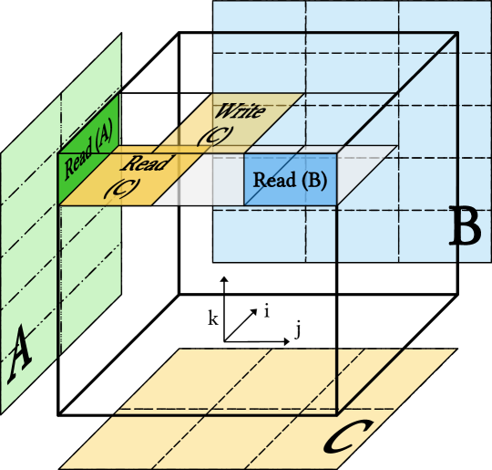
Figure 1. Tiled matrix product

In this example, an entire patch of each input matrix $A$, $B$ is transferred for the execution of each tile.

Despite the added locality, the application can still be memory-bound: tiled matrix product lacks data access contiguity. Barring any data layout manipulations, data is contiguous within a row (for row-major storage) or column (for column-major storage). A patch of $A$, $B$ or $C$ is never contiguous because it contains multiple parts of contiguous rows (or columns). The lack of contiguity therefore induces multiple short burst accesses to retrieve the entire patch.

Like for intermediate results, it is desirable to increase spatial locality and leverage contiguity to obtain higher performance on the input variables. Data blocking has been known to increase the performance of matrix multiplication, especially because data block correspond exactly to the “footprint” of iteration tiles on the matrix.

2.2. Limitations of existing transformations

Although data tiling is sufficient for matrix multiplication, more complex computational patterns require a finer data partitioning.

Ferry et al. (Ferry et al., 2023) proposes a breakup of intermediate results of programs with purely uniform dependence patterns, that enables contiguity. However, such dependence patterns exclude commonly found affine dependences, such as the broadcast-type dependences of matrix multiplication, despite there existing a natural breakup like data blocking.

Moreover, automatic data blocking is mostly applied by domain-specific compilers that have to generate the memory allocation (e.g. Halide (Ragan-Kelley et al., 2013), AlphaZ (Yuki et al., 2012)). When there exists a memory allocation and data layout in the input code, compilers follow it unless specific directives (e.g. the ARRAY_PARTITION directive in FPGA high-level synthesis tools based on (Cong et al., 2011)) are given to them. Allowing the compiler to change this allocation would open the door to better bandwidth utilization. Works on inter-node communication (Dathathri et al., 2013; Zhao et al., 2021) where memory allocation only exists within the nodes (and not across nodes) can resort to very specific groupings of data to minimize the communication overhead; it makes sense to apply this idea likewise to host-to-accelerator communications, despite there existing a global memory allocation.

In this work, we generalize the principle of data blocking to automatically partition the data arrays in function of when (in time) they are consumed. This approach can only be guaranteed to work with a specific class of programs called polyhedral programs where the exact data flow is known using static analysis.

In the same approach, we propose a secondary partitioning of the intermediate results; notably, this generalization coincides with an extension of the scope of previous work (Ferry et al., 2023) to affine dependences.

3. Background

We propose an automated approach to partitioning the data flow of a program. To construct it, we rely the polyhedral analysis and transformation framework and elements of linear algebra that this section introduces.

3.1. Polyhedral representation, tiling

To be eligible for affine MARS partitioning, a program (or a section thereof) must have a polyhedral representation. It may come either from the analysis of an imperative program (e.g. using PET (Verdoolaege and Grosser, 2012) or Clan (Bastoul et al., 2003)) or a domain-specific language. In any case, the following elements are assumed to be available:

• A $d$-dimensional iteration domain $\mathcal{D}\subset\mathbf{Z}^{d}$, or a collection of such domains,

• A $k$-dimensional data domain $\mathcal{A}$,

• A collection $(\varphi_{i})_{i}$ of access functions $\varphi_{i}:\mathcal{D}\to\mathcal{A}$, defining the reads and writes at each instance,

• A polyhedral reduced dependence graph (PRDG), constructed e.g. via array dataflow analysis (Feautrier, 1991).

The core elements extracted from the polyhedral representation are the dependences, that model which data must be available for a computation (any point in $\mathcal{D}$) to take place. The data flow notably comprises two kinds of dependences we focus about in this paper:

• Flow dependences: correspond to passing of intermediate results within the polyhedral section of the program,

• Input dependences: correspond to input data going into the program.

Both can be mapped to affine functions corresponding to the following definition:

Definition 3.1.

A dependence function is any affine function from an iteration domain $\mathcal{D}$ to another domain $\mathcal{D}^{\prime}$ (iteration or data). In particular, a dependence function is a single-valued relation (each element of $\mathcal{D}$ has a single image).

Each dependence will be noted $B$, and as an affine function, it is computed as $B(\vec{x})=A\vec{x}+\vec{b}$ with $A$ a matrix and $\vec{b}$ a vector.

Each domain is a subset of a Euclidean vector space $E\subset\mathbf{Z}^{d}$. In particular, every point $x\in\mathcal{D}$ is associated to a vector $\vec{x}\in E$. Section 3.2 gives further elements of linear algebra used throughout this paper.

Definition 3.2.

A dependence $B(\vec{x})=A\vec{x}+\vec{b}$ is said to be uniform when $A$ is the square identity matrix. A collection of dependences $B_{1},\dots,B_{n}$ are uniformly intersecting if they all have the same linear part, i.e. the same $A$ matrix.

To create a partitioning of the data spaces, our work relies on an existing partitioning of the iteration space. Loop tiling (Irigoin and Triolet, 1988; Schreiber and Dongarra, 1990; Wolf and Lam, 1991; Ramanujam and Sadayappan, 1992), a locality optimization, creates such a partitioning. It uses tiling hyperplanes to do so. Each hyperplane is defined by a normal vector (of unit norm). Tiles are periodically repeated, with a period $s$ called the tile size. We notably use scaled normal vectors that translate a point from a tile to the same point in another tile by crossing one tiling hyperplane.

In this work, we assume tiling hyperplanes are linearly independent from each other. Each tile has (unique) coordinates that are represented by a $t$-dimensional vector $\vec{t}=(i_{1},\dots,i_{t})$ where $t$ is the number of tiling hyperplanes. This tile is the set defined by

$$T(\vec{t})=\left\{\vec{x}\in E:\bigwedge_{j\in\{1,\dots,t\}}s_{j}i_{j}\leqslant\frac{1}{s_{j}}(\vec{x}\cdot\vec{n}_{j})<s_{j}(1+i_{j})\right\}$$

The footprint of a dependence $B$ and a tile $T(\vec{t})$ is the image of the tile by the dependence:

$$B\left<T(\vec{t})\right>=\left\{B(\vec{x}):x\in T(\vec{t})\right\}$$

3.2. Linear algebra

In this paper, we use several fundamental results from linear algebra. Below are reminders of them for the reader’s reference.

3.2.1. Spaces and bases

Definition 3.3.

Let $E$ be an Euclidean vector space of $d$ dimensions with its scalar product noted $\vec{x}\cdot\vec{y}$. Let $\mathcal{B}=\left(\vec{e}_{1},\dots,\vec{e}_{d}\right)$ be a basis of $E$. $\mathcal{B}$ is called an orthonormal basis of $E$ when for all $i\neq j$, $\vec{e}_{i}\cdot\vec{e}_{j}=0$ and for all $i$, $\vec{e}_{i}\cdot\vec{e}_{i}=1$.

Proposition 3.4.

Any Euclidean space $E$ of $d$ dimensions admits an orthonormal basis.

The proof of Proposition 3.4 is done by applying the Gram-Schmidt basis orthonormalization to an existing basis.

Definition 3.5.

The vector space of all linear combinations of a number of vectors $(\vec{e}_{1},\dots,\vec{e}_{n})$ is noted $\mathsf{vect}(\vec{e}_{1},\dots,\vec{e}_{n})$. Notably, that space has up to $n$ dimensions, and exactly $n$ dimensions if all the $n$ vectors are linearly independent.

Definition 3.6.

Two subspaces $S_{1}$ and $S_{2}$ of a vector space $E$ are supplementary into $E$ when their intersection is the null vector $\vec{0}$, and there exists a decomposition of all $\vec{x}\in E$ as $\vec{x}_{1}+\vec{x}_{2}$ with $\vec{x}_{1}\in S_{1}$ and $\vec{x}_{2}\in S_{2}$. That decomposition is notably unique.

3.2.2. Linear applications

Definition 3.7.

Let $A:E\to F$ be a linear application. The subspace $K$ of $E$ such that $\forall\vec{x}\in K,A\vec{x}=\vec{0}$ is called the null space of $A$ and is noted $\mathsf{ker}(A)$.

Definition 3.8.

Let $A:E\to F$ be a linear application. The image of $E$ by $A$ is noted $A\left<E\right>$. Likewise, the image of a subspace $S\subset E$ by $A$ is noted $A\left<G\right>$. The preimage of a subspace $T\subset F$ is noted $A^{-1}\left<F\right>$.

Proposition 3.9.

If $A:E\to F$ is a linear application, $E$ has $d$ dimensions, and $\mathsf{ker}(A)$ is its null space, then let $k\leqslant d$ be the dimensionality of $\mathsf{ker}(A)$. There exists a $d-k$-dimensional supplementary $I$ of $\mathsf{ker}(A)$ in $E$, such that:

$$\forall\vec{x}\in I,(A\vec{x}=\vec{0}\Rightarrow\vec{x}=\vec{0})$$

4. Partitioning Data and Iteration Spaces

This section constitutes the core of our work: it proposes a breakup of the iteration and data spaces based on the same properties as the existing uniform breakup, detailed in Section 4.1.

The reasoning leading to the MARS starts from a simple, restrictive case (one single dependence, Section 4.3) and progressively relaxes its hypotheses (multiple uniformly intersecting dependences, Section 4.4 and non-uniformly intersecting dependences, Section 4.5). The last step of the reasoning in Section 4.6 adds the constraint of partitioning an existing tiled space, which allows to partition intermediate results.

4.1. Case of uniform dependences

Maximal Atomic irRedundant Sets (MARS) are introduced in (Ferry et al., 2023). They are defined as a partition of the flow-out iterations of a tile, such that every element of the partition is the largest set of iterations that verifies:

• Atomicity: consumption of a single element from a MARS implies consumption of the entire MARS.

• Maximality: considering all the consumers of a MARS $M_{0}$ ($C_{0}$) and all the consumers of another MARS $M_{1}$ ($C_{1}$), if $C_{0}=C_{1}$, then $M_{0}=M_{1}$.

• Irredundancy: each element of the MARS space belongs to no more than a single MARS.

While (Ferry et al., 2023) uses the flow-in and flow-out information in the sense of (Bondhugula, 2013), input data and output data do not belong to this information. This work instead resorts on the notion of footprint from (Agarwal et al., 1995); notably, the notion of flow-in iterations of a tile coincides with that of a footprint of a tile (of iterations) on another tile of iterations.

The properties of MARS constructed with uniform dependences are the same as those sought in this paper. Merely proposing a partition of the iteration or data spaces satisfies the irredundancy property; the properties to actually check from the partitioning are the atomicity and maximality.

4.2. The problem: uniform versus affine dependences

In the uniform case, MARS can be constructed by enumerating all the consumer tiles of a given tile, i.e. those other tiles that need data from that tile. The uniformity guarantees that there are a finite number of consumer tiles, and that all tiles will exhibit the same MARS regardless of their position in the iteration space (i.e. MARS are invariant by translation of a tile).

Affine dependences do not guarantee a finite number of consumer tiles; it may be parametric or potentially unbounded. Also, it becomes necessary to assert when the invariance by translation is possible.

In the rest of this section, we will prove, for one and multiple dependences:

• The existence of a finite set of representatives of all consumer tiles, suitable to determine the MARS partition,

• The invariance of the partitioning by a translation of a tile, or conditions to guarantee it.

4.3. Case of a single affine dependence

The simplest case is when there is a single affine dependence between a tiled iteration space and a data space. This subsection starts with an example and explains the general case afterwards.

4.3.1. Example

To start with, we introduce an example with a single dependence, and non-canonical tiling hyperplanes.

• Domain: $\left\{(i,j):0\leqslant i<N,0\leqslant j<M\right\}$, basis vectors $\vec{e}_{i},\vec{e}_{j}$

• Dependence : $S_{0}(i,j)\mapsto\mathcal{A}(i)$, represented as $B(i,j)=(i)$ (i.e. $B(\vec{x})=A\vec{x}+\vec{b}$ with $A:(i,j)\mapsto(i)$ and $\vec{b}=\vec{0}$).

• Tiling hyperplanes : $H_{0}:i+j$, $H_{1}:j-i$

• Normal vectors: $\vec{n}_{1}=(1,1)$, $\vec{n}_{2}=(-1,1)$; scaled normal vectors (w.r.t. tile size): $\vec{\mathbf{n}}_{1}=(s/2,s/2)$, $\vec{\mathbf{n}}_{2}=(-s/2,s/2)$

• Tile size : $s\in\mathbf{N}^{*}$

We want to construct the MARS on the $\mathcal{A}$ data space. To do so, we are going to compute the footprint (Agarwal et al., 1995) of a tile onto the data space along the dependence $B$; then, by noticing that all footprints are a translation of the same footprint, we will determine parametrically which tiles have intersecting footprints, and compute the MARS using the same method as (Ferry et al., 2023).

We first define a tile of iterations with a parametric set : we call $T(i_{0},i_{1})$ the set :

$$T(i_{0},i_{1})=\left\{(i,j):si_{0}\leqslant i+j<s(1+i_{0})\wedge si_{1}\leqslant j-i<s(1+i_{1})\right\}$$

The footprint of $T(i_{0},i_{1})$ by the dependence $B$, appearing in Figure 2, is therefore:

$$B\left<T(i_{0},i_{1})\right>=\left\{(i):\exists j:si_{0}\leqslant i+j<s(1+i_{0})\wedge si_{1}\leqslant j-i<s(1+i_{1})\right\}$$

where the existential quantifier may be removed:

$$B\left<T(i_{0},i_{1})\right>=\left\{(i):s(i_{0}-i_{1}-1)<2i<s(i_{0}-i_{1}+1)\right\}$$

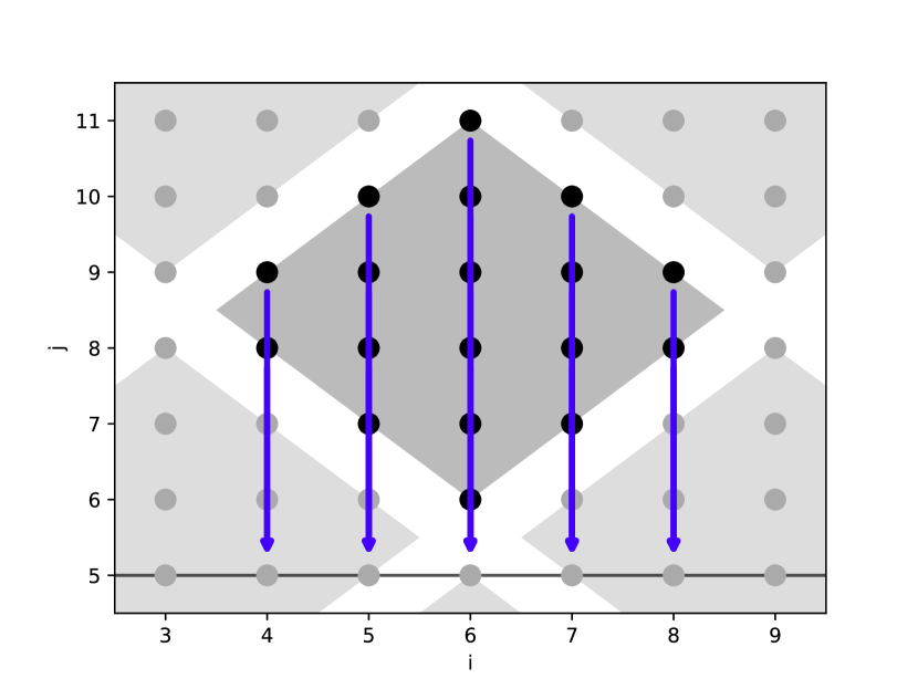
Figure 2. Footprint of one tile with a single affine dependence $B(i,j)=(i)$. The one-dimensional destination space is shown as a continuous line.

Given $(i_{0},i_{1})$, we now seek the other tiles which footprint’s intersection with $B\left<T(i_{0},i_{1})\right>$ is not empty: let $(i_{2},i_{3})$ be another tile.

$$B\left<T(i_{0},i_{1})\right>\cap B\left<T(i_{2},i_{3})\right>=$$

$$\left\{(i):s(i_{0}-i_{1}-1)+1\leqslant 2i\leqslant s(i_{0}-i_{1}+1)-1\right.$$

$$\left.\wedge s(i_{2}-i_{3}-1)+1\leqslant 2i\leqslant s(i_{2}-i_{3}+1)-1\right\}$$

The intervals $\left[\!\left[s(i_{0}-i_{1}-1)+1;s(i_{0}-i_{1}+1)-1\right]\!\right]$ and
$\left[\!\left[s(i_{2}-i_{3}-1)+1;s(i_{2}-i_{3}+1)-1\right]\!\right]$ intersect if $i_{0}-i_{1}=i_{2}-i_{3}+1$, $i_{0}-i_{1}=i_{2}-i_{3}$ or $i_{0}-i_{1}=i_{2}-i_{3}-1$.

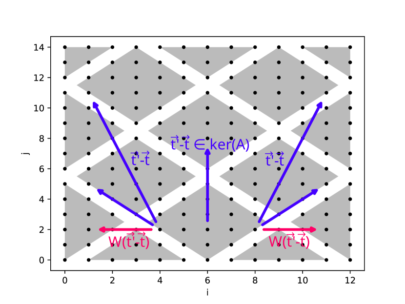
Figure 3. Some consumer tiles of one tile $T(\vec{t})$ with a single dependence $B(i,j)=(i)$, and the projection $W(\vec{t^{\prime}}-\vec{t})$ on a supplementary of $\mathsf{ker}(A)$. There are a finite number of such projected vectors, and they are constant.

The valid $(i_{2},i_{3})$s are therefore:

$$(i_{2},i_{3}) \in\left\{(i_{0}+p,i_{1}+p);p\in\mathbf{Z}\right\}$$

$$\cup\left\{(i_{0}+p-1,i_{1}+p);p\in\mathbf{Z}\right\}$$

$$\cup\left\{(i_{0}+p+1,i_{1}+p);p\in\mathbf{Z}\right\}$$

as shown in blue in Figure 3.

The space of valid $(i_{2},i_{3})$ is infinite: we can visually see this as all tiles along a vertical axis share the same footprint on $\mathcal{A}$. We can formalize this intuition by computing the kernel of $A$ : in this case, it is

$$\mathsf{ker}(A)=\mathsf{vect}(\vec{e}_{j})$$

and the image of a point on $\mathcal{A}$ is invariant by any upwards or downwards translation.

There are however only three distinct footprints intersecting with that of $T(i_{0},i_{1})$; the other footprints stem from tiles which are translations along $\mathsf{ker}(A)$. These footprints come from the top-left, top-right tiles and all tiles above them vertically; these consumer tiles are shown in Figure 3.

We can decompose the space $(i,j)$ using a basis of the kernel and a supplementary, for instance $E=\mathsf{vect}(\vec{e}_{i})\oplus\mathsf{ker}(A)$.

In this basis, we can express the coordinates of tile’s origins for the case where $(i_{2},i_{3})=(i_{0}+p+1,i_{1}+p)$ with $p\in\mathbf{Z}$ using the scaled normal vectors $\vec{\mathbf{n}}_{1}$, $\vec{\mathbf{n}}_{2}$:

$$i_{2}\vec{\mathbf{n}}_{1}+i_{3}\vec{\mathbf{n}}_{2} =i_{2}\frac{s}{2}(\vec{e}_{i}+\vec{e}_{j})+i_{3}\frac{s}{2}(\vec{e}_{j}-\vec{e}_{i})$$

$$=\frac{s}{2}(i_{0}+p+1)(\vec{e}_{i}+\vec{e}_{j})+\frac{s}{2}(i_{1}+p)(\vec{e}_{j}-\vec{e}_{i})$$

$$=\frac{s}{2}(i_{0}-i_{1}+1)\vec{e}_{i}+\frac{s}{2}(i_{0}+i_{1}+2p+1)\vec{e}_{j}$$

which, when projected onto $\mathsf{vect}(\vec{e}_{i})$, gives:

$$P_{\mathsf{vect}(\vec{e}_{i})}(i_{2}\vec{\mathbf{n}}_{1}+i_{3}\vec{\mathbf{n}}_{2})=\frac{s}{2}(i_{0}-i_{1}+1)\vec{e}_{i}$$

which is independent of $p$. This means that all points within tile $T(i_{2},i_{3})$ have the same image by $B$. Therefore, given $(i_{0},i_{1})$, the entire family of tiles $(i_{0}+p+1,i_{1}+p)$ have the same footprint on $\mathcal{A}$. We can therefore consider a single representative of that family to compute the MARS.

Likewise, if $(i_{2},i_{3})=(i_{0}+p-1,i_{1}+p)$ with $p\in\mathbf{Z}$, then

$$P_{\mathsf{vect}(\vec{e}_{i})}(i_{2}\vec{\mathbf{n}}_{1}+i_{3}\vec{\mathbf{n}}_{2})=\frac{s}{2}(i_{0}-i_{1}-1)\vec{e}_{i}$$

which is also independent of $p$; the same conclusion holds for $(i_{2},i_{3})=(i_{0}+p,i_{1}+p)$ and $P_{\mathsf{vect}(\vec{e}_{i})}(i_{2}\vec{\mathbf{n}}_{1}+i_{3}\vec{\mathbf{n}}_{2})=\vec{0}$. Figure 3 shows in pink the projection of the translation vectors from the tile $T(\vec{t})$ to its consumers (there are only two non-null projections, so only two such vectors appear).

There are an infinity of tiles which footprint intersects with that of a given tile; however, to compute the MARS, we have demonstrated that it is sufficient to take three representative tiles. The same procedure as in (Ferry et al., 2023) can be applied once these three consumer tiles have been determined.

Per (Ferry et al., 2023), we compute the respective intersections with $B\left<T(i_{0},i_{1})\right>$ of all other consumer tiles: for $(i_{2},i_{3})=(i_{0}+p+1,i_{1}+p)$ with $p\in\mathbf{Z}$,

$$B\left<T(i_{0},i_{1})\right>\cap B\left<T(i_{0}+p+1,i_{1}+p)\right>=$$

$$\left\{(i):s(i_{0}-i_{1}-1)<2i<s(i_{0}-i_{1}+1)\right.$$

$$\left.\wedge s(i_{0}-i_{1})<2i<s(i_{0}-i_{1}+2)\right\}$$

$$=\left\{(i):s(i_{0}-i_{1})<2i<s(i_{0}-i_{1}+1)\right\}$$

When $(i_{2},i_{3})=(i_{0}+p-1,i_{1}+p)$ with $p\in\mathbf{Z}$,

$$B\left<T(i_{0},i_{1})\right>\cap B\left<T(i_{0}+p-1,i_{1}+p)\right>=$$

$$=\left\{(i):s(i_{0}-i_{1}-1)<2i<s(i_{0}-i_{1})\right\}$$

Finally, when $(i_{2},i_{3})=(i_{0}+p,i_{1}+p)$,

$$B\left<T(i_{0},i_{1})\right>\cap B\left<T(i_{0}+p,i_{1}+p)\right>=$$

$$=\left\{(i):s(i_{0}-i_{1})=2i\right\}$$

Also, $B\left<T(i_{0}+p+1,i_{1}+p)\right>\cap B\left<T(i_{0}+p-1,i_{1}+p)\right>=\varnothing$, so we have all the MARS.

The MARS on symbol $\mathcal{A}$ for this program seen from a tile $T(i_{0},i_{1})$ are therefore the three sets $\left\{(i):s(i_{0}-i_{1})<2i<s(i_{0}-i_{1}+1)\right\}$, $\left\{(i):s(i_{0}-i_{1}-1)<2i<s(i_{0}-i_{1})\right\}$ and $\left\{(i):s(i_{0}-i_{1})=2i\right\}$. These MARS are shown in Figure 4.

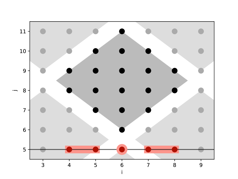
Figure 4. MARS obtained with a single affine dependence $B(i,j)=(i)$.

4.3.2. General case

In the general case, computing the MARS for a single dependence leading to a non-tiled space can be done as follows. Let $\mathcal{D}$ be the $N$-dimensional iteration space from which the dependence originates, and $E$ be the vector space such that $\mathcal{D}\subset E$.; let $\mathcal{A}$ be the destination space. Let $B$ be the dependence with $B(\vec{x})=A\vec{x}+\vec{b}$. Let $(H_{1},\dots,H_{t})$ be the $t$ tiling hyperplanes, $(\vec{n}_{1},\dots,\vec{n}_{t})$ normal vectors to the tiling hyperplanes, $(s_{1},\dots,s_{t})$ be the tile sizes.

For a tile coordinate be $\vec{t}=(i_{1},\dots,i_{t})$, the tile is defined as

$$T(\vec{t})=\left\{\vec{x}=(x_{1},\dots,x_{N}):\forall j\in\{1,\dots,t\}:s_{j}i_{j}\leqslant\vec{x}\cdot\vec{n}_{j}<s_{j}(1+i_{j})\right\}$$

We can compute, with $\vec{t}$ and another tile $\vec{t^{\prime}}$ as a parameter, when the intersection of $B\left<T(\vec{t})\right>$ and $B\left<T(\vec{t^{\prime}})\right>$ is non-empty using affine operations. Let $V(\vec{t})$ be:

$$V(\vec{t})=\left\{\vec{t^{\prime}}:B\left<T(\vec{t})\right>\cap B\left<T(\vec{t^{\prime}})\right>\neq\varnothing\right\}$$

which is obtainable by taking the parameter space of $I(\vec{t},\vec{t^{\prime}})$. $V(\vec{t})$ represents the tile coordinates of all tiles which footprint on $\mathcal{A}$ intersects that of $T(\vec{t})$.

In (Ferry et al., 2023), $V(\vec{t})$ is determined by browsing through neighboring tiles. The main difficulty here is that $V(\vec{t})$ is potentially infinite. We will demonstrate that there are only a finite number of distinct footprints overlapping with $B\left<T(\vec{t^{\prime}})\right>$. To determine them, we suggest to decompose $E$ into $\mathsf{ker}(A)$ and a supplementary $I$ of $\mathsf{ker}(A)$, i.e.

$$E=I\oplus\mathsf{ker}(A)$$

Proposition 3.9 gives us that such a decomposition always exists, and per Proposition 3.4, there is an orthonormal basis of the resulting space.

If $r=\mathsf{rank}(A)$, let $(\vec{e}_{1},\dots,\vec{e}_{r})$ be a basis of $I$ and $(\vec{e}_{r+1},\dots,\vec{e}_{d})$ be a basis of $\mathsf{ker}(A)$ such that $(\vec{e}_{1},\dots,\vec{e}_{d})$ is an orthonormal basis of $E$. Let $(\vec{n}^{p}_{1},\dots,\vec{n}^{p}_{t})$ be the orthogonal projections of the $\vec{n}_{i}$s onto $(\vec{e}_{1},\dots,\vec{e}_{r})$; in particular, these have zero $r+1$-th through $d$-th coordinates.

For any $\vec{t^{\prime}}\in V(\vec{t})$, if $\vec{t^{\prime}}-\vec{t}=(\delta_{1},\dots,\delta_{t})$, we can compute

$$W(\vec{t^{\prime}}-\vec{t})=\sum_{i=1}^{t}\delta_{i}\vec{n}^{p}_{i}$$

which represents the part of the translation between tiles that results in translating the images.

The most important result needed to construct the MARS is the ability to enumerate all the footprints. The following proposition formalizes it:

Proposition 4.1.

The set $P(\vec{t})=\left\{W(\vec{t^{\prime}}-\vec{t}):\vec{t^{\prime}}\in V(\vec{t})\right\}$ is finite, and for each consumer tile $\vec{t^{\prime}}\in V(\vec{t})$, there exists a unique $\vec{p}\in P(\vec{t})$ such that

$$B\left<T(\vec{t^{\prime}})\right>=\left\{\vec{y}+A\vec{p}:\vec{y}\in B\left<T(\vec{t})\right>\right\}$$

and that $\vec{p}$ is a constant vector, independent of $\vec{t}$ (i.e. the consumer tiles are invariant by translation).

Proof.

Completeness of footprints: Let $\vec{t^{\prime}}\in V(\vec{t})$, i.e. a tile which footprint intersects that of tile $\vec{t}$. We know that $W(\vec{t^{\prime}}-\vec{t})=\sum_{i=1}^{t}(t^{\prime}_{i}-t_{i})\vec{n}^{p}_{i}=\vec{p}\in P(\vec{t})$. Then:

$$B\left<T(\vec{t^{\prime}})\right> =\left\{A\vec{x}+\vec{b}:\forall i:s_{i}t^{\prime}_{i}\leqslant\vec{x}\cdot\vec{n}_{i}\leqslant(1+t^{\prime}_{i})s_{i}\right\}$$

$$=\left\{A\vec{x}+\vec{b}:\forall i:s_{i}(t_{i}+(t^{\prime}_{i}-t_{i}))\leqslant\vec{x}\cdot\vec{n}_{i}\leqslant(1+t_{i}+(t^{\prime}_{i}-t_{i}))s_{i}\right\}$$

$$=\left\{A\left(\vec{x}+{\textstyle\sum_{i=1}^{t}}(t^{\prime}_{i}-t_{i})\vec{n}_{i}\right)+\vec{b}:\forall i:s_{i}t_{i}\leqslant\vec{x}\cdot\vec{n}_{i}\leqslant(1+t_{i})s_{i}\right\}$$

$$=\left\{A\left(\vec{x}+{\textstyle\sum_{i=1}^{t}}(t^{\prime}_{i}-t_{i}){\color[rgb]{1,0,0}\vec{n}^{p}_{i}}\right)+\vec{b}:\vec{x}\in T(\vec{t})\right\}$$

$$=\left\{\vec{y}+A\vec{p}:\vec{y}\in B\left<T(\vec{t})\right>\right\}$$

using the fact that ${\color[rgb]{1,0,0}A(\vec{n}_{i})=A(\vec{n}_{i}^{p})}$.

Uniqueness of $\vec{p}$: $A$ is bijective between $I$ (supplementary of $\mathsf{ker}(A)$ in $E$) and $\textsf{Im}(A)$. Therefore, because $\vec{p}\in P(\vec{t})$ is in $I$, it is the unique element of $I$ which $A\vec{p}$ is the image. Therefore, $\vec{p}$ is unique in the sense of this proposition.

Finiteness of $P(\vec{t})$: For all $\vec{t^{\prime}}\in V(\vec{t})$, $B\left<T(\vec{t^{\prime}})\right>$ is a translation of $B\left<T(\vec{t})\right>$ by $A\vec{p}$ with some $\vec{p}\in P(\vec{t})$. The coordinates of $\vec{t}$ are integers, therefore $A\vec{p}$ is an integer linear combination of the $A\vec{n}_{i}^{p}$s for $i\in\{1,\dots,t\}$. $T(\vec{t})$ being bounded, the footprint $B\left<T(\vec{t})\right>$ is bounded, therefore only a finite number of translations of itself by $A\vec{p}$s intersect with it.

Constantness of $\vec{p}$: Let $\vec{t}_{0},\vec{t}_{1}\in\mathbf{Z}^{t}$ and $\vec{t^{\prime}}_{0}\in V(\vec{t}_{0})$, and $\vec{p}=W(\vec{t^{\prime}}-\vec{t})$. Let $\vec{t^{\prime}}_{1}=\vec{t}_{1}+(\vec{t^{\prime}}_{0}-\vec{t}_{0})$. Then:

$$B\left<T(\vec{t^{\prime}}_{1})\right> =\left\{A\left(\vec{x}+{\textstyle\sum_{i=1}^{t}}(t^{\prime}_{1i}-t_{1i})\vec{n}_{i}\right)+\vec{b}:\forall i:s_{i}t_{1i}\leqslant\vec{x}\cdot\vec{n}_{i}\leqslant(1+t_{1i})s_{i}\right\}$$

$$=\left\{A\left(\vec{x}+{\textstyle\sum_{i=1}^{t}}(t_{1i}-t_{1i}+(t^{\prime}_{0i}-t_{0i}))\vec{n}_{i}\right)+\vec{b}:\vec{x}\in T(\vec{t}_{1})\right\}$$

$$=\left\{A\vec{x}+{\textstyle\sum_{i=1}^{t}}(t^{\prime}_{0i}-t_{0i})A\vec{n}_{i}+\vec{b}:\vec{x}\in T(\vec{t}_{1})\right\}$$

$$=\left\{B(\vec{x})+A\vec{p}:\vec{x}\in T(\vec{t}_{1})\right\}$$

which means that the translation between the images of $T(\vec{t}_{1})$ and $T(\vec{t^{\prime}}_{1})$ is the same as that of $T(\vec{t}_{0})$ and $T(\vec{t^{\prime}}_{0})$.

∎

We can therefore enumerate $P(\vec{t})$, knowing that for each $\vec{w}\in P(\vec{t})$, $P^{-1}(\vec{w})$ represents consumer tiles that all have the same footprint by $B$. That footprint is computed as follows:

$$\Phi(\vec{w})=B\left<T(\vec{t})+\vec{w}\right>\text{ where }T(\vec{t})+\vec{w}=\left\{\vec{x}+\vec{w}:\vec{x}\in T(\vec{t})\right\}$$

We can then compute the MARS. For all the combinations of $\vec{w}$s, i.e. for all $C\in\mathcal{P}\left(P(\vec{t})\right)$, we determine the MARS associated with that combination of consumer tiles:

$$\mathcal{M}_{C}=\bigcap_{\vec{w}\in C}\left(\Phi(\vec{w})\cap B\left<T(\vec{t})\right>\right)\setminus\bigcup_{\vec{w}\notin C}\left(\Phi(\vec{w})\cap B\left<T(\vec{t})\right>\right)$$

4.4. Case of multiple, uniformly intersecting dependences

4.4.1. General case

If the dependences are uniformly intersecting, they all have the same linear part. This means that they all have the same null space, and therefore the space decomposition into $E=I\oplus\mathsf{ker}(A)$ still applies.

Let there be $Q$ dependences $B_{1},\dots,B_{Q}$ that are uniformly intersecting. This means that there exists an unique matrix $A$ such that:

$$\forall i:B_{i}(\vec{x})=A\vec{x}+\vec{b}_{i}$$

Because all tiles share the same linear part, the space of consumer tiles for each dependence will be the same up to a translation. Their linear part will notably be the same, and the same argument as in the case above holds to guarantee that $P(\vec{t})=\left\{W(\vec{t^{\prime}}-\vec{t}):\vec{t^{\prime}}\in V(\vec{t})\right\}$ is finite.

Let, by abuse of the notation, $B\left<T(\vec{t})\right>$ be the combined footprint of all dependences:

$$B\left<T(\vec{t})\right>=\bigcup_{i=1}^{Q}B_{i}\left<T(\vec{t})\right>$$

For each dependence $B_{i}$ with $i\in\{1,\dots,Q\}$, we therefore compute $V_{i}(\vec{t})$ by intersecting $B_{i}\left<T(\vec{t^{\prime}})\right>$ and $B\left<T(\vec{t})\right>$ (i.e. we want the intersection of the footprint of one dependence and the footprint of all other dependences); let

$$V(\vec{t})=\bigcup_{i=1}^{Q}V_{i}(\vec{t})$$

The same decomposition $E=\mathsf{vect}(\vec{e}_{1},\dots,\vec{e}_{r})\oplus\mathsf{vect}(\vec{e}_{r}+1,\dots,\vec{e}_{d})$ is applicable due to all $B_{i}$s sharing the same linear part $A$.

We can give a more meaningful expression for $P(\vec{t})$:

$$P(\vec{t})=\left\{W(\vec{t^{\prime}}-\vec{t}):\vec{t^{\prime}}\in\bigcup_{i=1}^{Q}V_{i}(\vec{t})\right\}$$

which means that $P(\vec{t})$ is composed of the projections of the vectors leading to any consumer tile of any dependence (and therefore takes into account the uniform translations between dependences).

The MARS can be computed by using $P(\vec{t})$. There are two differences with the case when there is only a single dependence:

• The footprints of the consumer tiles $\Phi(\vec{w})$ are specific to each dependence,

• The footprint of the tile $\vec{t}$ is the union of the footprint of all dependences.

For $i\in\{1,\dots,Q\}$, let $\Phi_{i}(\vec{w})$ be:

$$\Phi_{i}(\vec{w})=B_{i}\left<T(\vec{t})+\vec{w}\right>\text{ where }T(\vec{t})+\vec{w}=\left\{\vec{x}+\vec{w}:\vec{x}\in T(\vec{t})\right\}$$

The MARS are constructed by taking all subsets of consumer tiles from $P(\vec{t})$, and looking at the points consumed only by these tiles.

Formally, let the cardinality of $P(\vec{t})$ be $\#C$. For all $K:1\leqslant K\leqslant\#C$ and all permutations $\sigma$ of $\{1,\dots,\#C\}$, let

$$C=\left\{\vec{t}_{\sigma(1)},\dots,\vec{t}_{\sigma(K)}\right\}\text{ and }\overline{C}=\{\vec{t}_{\sigma(K+1)},\dots,\vec{t}_{\sigma(\#C)}\}$$

Then, a MARS is constructed according to the following rules:

• For each consumer tile coordinates $\vec{t^{\prime}}\in C$, there exists a dependence leading to $T(\vec{t^{\prime}})$,

• No dependence leads to a consumer tile $\vec{t^{\prime}}\in\overline{C}$

These two conditions to form a MARS can be written as:

$$\mathcal{M}_{C}=\bigcap_{\vec{w}\in C}\left(\bigcup_{i=1}^{Q}\Phi_{i}(\vec{w})\cap B\left<T(\vec{t})\right>\right)\setminus\bigcup_{\vec{w}\in\overline{C}}\left(\bigcup_{i=1}^{Q}\Phi_{i}(\vec{w})\cap B\left<T(\vec{t})\right>\right)$$

and there are at most $\mathsf{card}(\mathcal{P}(P(\vec{t})))=2^{\mathsf{card}(P(\vec{t}))}$ $C$s and therefore as many MARS.

4.4.2. Example: uniform dependences

In this paragraph, we show that the computation of MARS using (Ferry et al., 2023) coincides with that proposed in this paper when the dependences are uniform. Such dependences are a special case of uniformly intersecting dependences, with a linear part being identity. Note that the destination space is considered to be a data space, and therefore dependences within a tile are counted in the footprint (self-consumption of data produced by a tile is dealt with in the next section).

Consider the Jacobi 1D example:

• Domain: $\left\{(i,j):0\leqslant i<N,0\leqslant j<M\right\}$, basis vectors $\vec{e}_{i},\vec{e}_{j}$

• Dependences : $B_{1}(i,j)=(i-1,j-1)$, $B_{2}(i,j)=(i,j-1)$, $B_{3}(i,j)=(i+1,j-1)$

• Tiling hyperplanes : $H_{1}:i+j$ ($\vec{n}_{2}=(1,1)$), $H_{2}:j-i$ ($\vec{n}_{2}=(-1,1)$)

• Tile size : $s\in\mathbf{N}^{*}$

We compute the unified footprint $B\left<T(\vec{t})\right>$:

$$B\left<T(\vec{t})\right>=\left\{(i,j):si_{1}\leqslant i+j+(2-p)<s(1+i_{1})\right.$$

$$\left.\wedge si_{2}\leqslant j-i+p<s(1+i_{2}):p\in\{0,1,2\}\right\}$$

Notably, if we confuse the data space $\mathcal{A}(i,j)$ and the iteration space $(i,j)$ (that is, each cell of $\mathcal{A}$ contains the result of one iteration), and we restrict the footprint to those points outside tile $T(\vec{t})$, we obtain the flow-in of that tile as in Figure 5, corresponding to the same definition as in (Ferry et al., 2023).

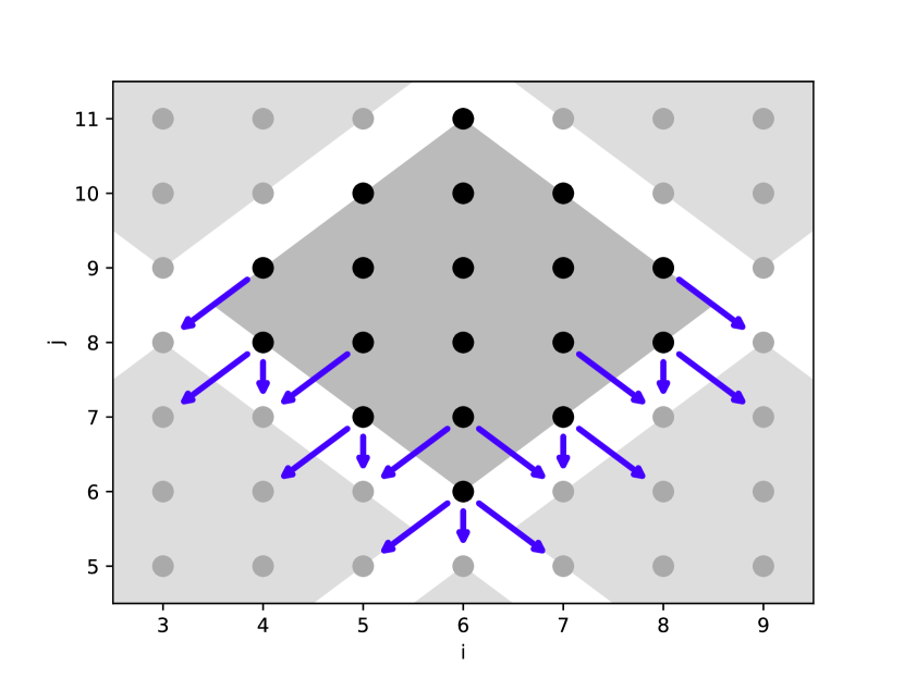
Figure 5. Flow-in dependences of tile $T(\vec{t})$ with uniformly intersecting dependences (Jacobi 1D).

We determine the individual $V_{i}(\vec{t})$s:

$$V_{1}(\vec{t}) =\left\{(i_{1},i_{2}-1),(i_{1},i_{2}),(i_{1}+1,i_{2}-1),(i_{1}+1,i_{2})\right\}$$

$$V_{2}(\vec{t}) =\left\{(i_{1},i_{2}),(i_{1}+1,i_{2}),(i_{1},i_{2}-1),(i_{1}-1,i_{2}),(i_{1},i_{2}+1)\right\}$$

$$V_{3}(\vec{t}) =\left\{(i_{1},i_{2}),(i_{1}-1,i_{2}),(i_{1},i_{2}+1),(i_{1}-1,i_{2}+1)\right\}$$

which gives

$$V(\vec{t})= \left\{(i_{1},i_{2}),(i_{1}-1,i_{2}),(i_{1},i_{2}+1),(i_{1}-1,i_{2}+1),(i_{1}+1,i_{2}),\right.$$

$$\left.(i_{1},i_{2}-1),(i_{1}+1,i_{2}-1)\right\}$$

As $\mathsf{ker}(A)=\{0\}$, we easily get that $E=\mathsf{vect}(\vec{e}_{i},\vec{e}_{j})$ and therefore constructing the $W(\vec{t^{\prime}}-\vec{t})$ is straightforward, yielding the following $P(\vec{t})$:

$$P(\vec{t})=\left\{(0,0),(-1,0),(0,1),(-1,1),(1,0),(0,-1),(1,-1)\right\}$$

This $P(\vec{t})$ means there are seven tiles (including $\vec{t}$ itself) which footprint (i.e. any dependence) intersects with $B\left<T(\vec{t})\right>$. These consumer tiles are shown in Figure 6.

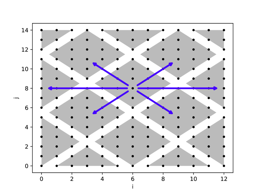
Figure 6. Consumer tiles of array $\mathcal{A}$ with Jacobi 1D dependences, sharing their footprint with tile $T(\vec{t})$.

For the sake of shortness, we will not enumerate all combinations of consumer tiles. The MARS that appear after partitioning the footprints stemming from all consumer tiles are shown in Fig.7.

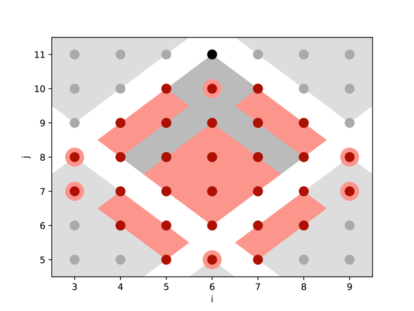
Figure 7. MARS for uniformly intersecting dependences (Jacobi 1D)

Again, if we confuse the iteration and data spaces, we can obtain the same MARS as computed in (Ferry et al., 2023) by removing those MARS that are contained within $T(\vec{t})$; the result of this operation, shown in Figure 8, illustrates the coincidence between the MARS computed using uniform and affine dependences.

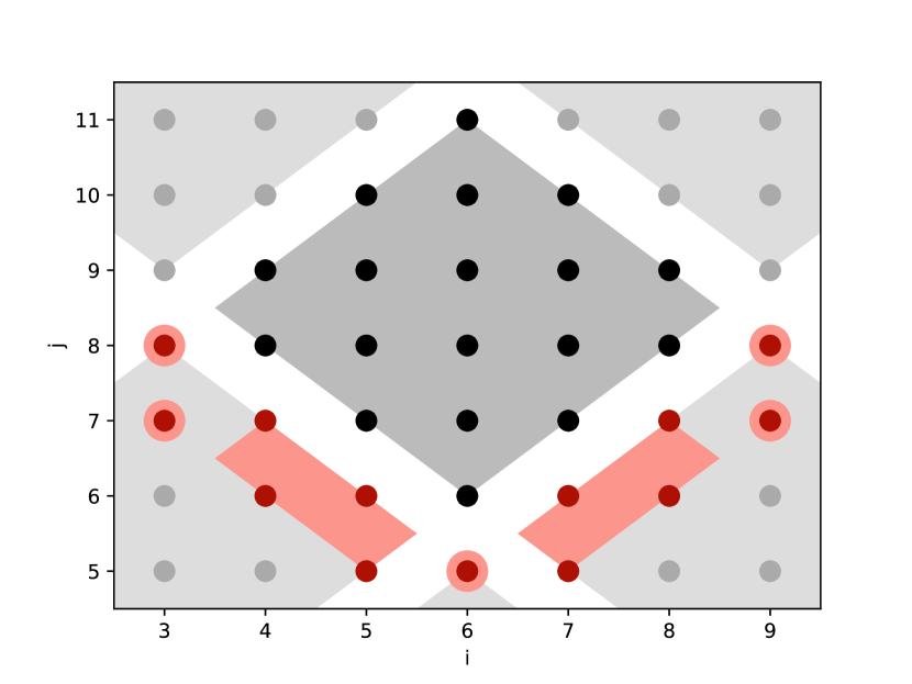
Figure 8. Coincidence between MARS computed with the uniform dependence method, and those computed with the affine method.

4.5. Case of multiple, non-uniformly intersecting dependences

We now consider the case where the dependences are not uniformly intersecting. In this case, the main difference is that dependences no longer share the same linear part. Therefore, we need to write every dependence separately:

$$\forall i\in\{1,\dots,Q\}:B_{i}(\vec{x})=A_{i}\vec{x}+\vec{b}_{i}$$

and each dependence having its own null space, there is one orthonormal basis of the null space and a supplementary per dependence, and therefore one projection $W_{i}(\vec{t^{\prime}}-\vec{t})$ per dependence.

4.5.1. Single null space requirement

Because the dependences may no longer have the same linear part, each linear part may have a different null space. When considering any consumer tile $\vec{t^{\prime}}\in V(\vec{t})$, it is no longer true that the projection of $\vec{t^{\prime}}-\vec{t}$ onto each null space is independent of the tile coordinates. The invariance by translation of a tile from Proposition 4.1 therefore no longer holds.

Figure 9 gives an example of this case with two dependences: $B_{1}(i,j)=(i-j)$ and $B_{2}(i,j)=(i+j)$. Here, the $\vec{p}$s depend on $\vec{t}$. Due to the dependence $B_{1}$, all the tiles northwest of each tile will intersect with its footprint; but the dependence $B_{2}$ generates a footprint southwest, also consumed (because of $B_{1}$) by all tiles to its northwest.

In Figure 9, we show the $W_{1}(\vec{t^{\prime}}-\vec{t})$ : $\ker(A_{1})$ points to the northeast, and $I_{1}$ (supplementary of $\ker(A_{1})$) points to the northwest, parallel to the dependence $B_{2}$.

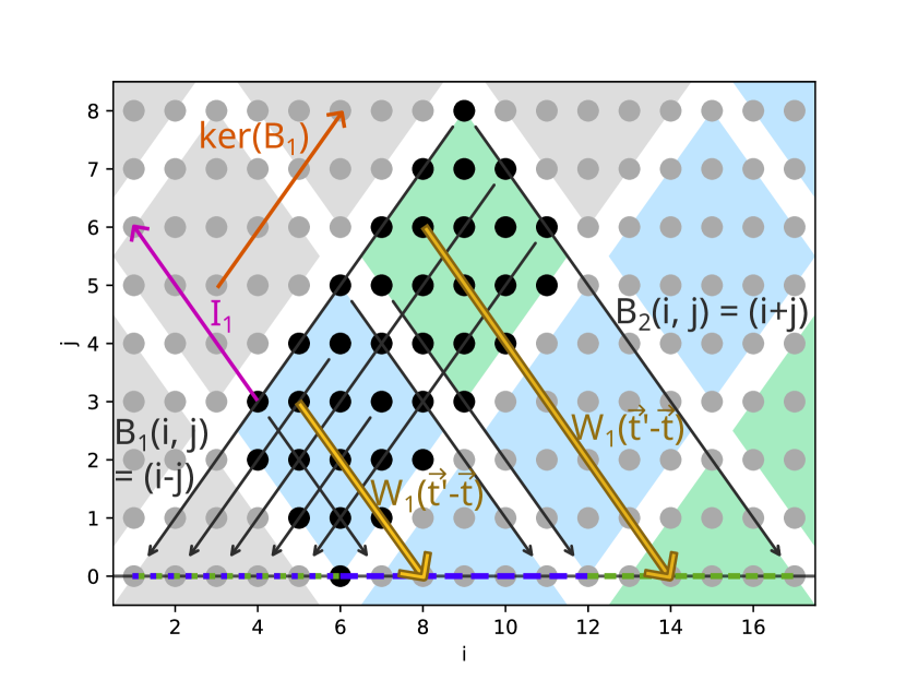
Figure 9. Non-uniformly intersecting dependences do not guarantee that the vectors $W_{i}(\vec{t^{\prime}}-\vec{t})$ do not depend on $\vec{t}$, i.e. each tile’s footprint is not necessarily a translation of another tile’s footprint.

A sufficient condition for a position-independent footprint to exist is that all dependences have the same null space:

Proposition 4.2.

If all dependences have the same null space, then all tiles have the same footprint up to a translation. Otherwise said, for any $\vec{\delta}\in\mathbf{Z}^{t}$, there exists $\vec{u}\in\mathsf{Im}(B)$ such that:

For each $\vec{t}\in\mathbf{Z}^{t}$, if $\vec{t^{\prime}}=\vec{t}+\vec{\delta}$, then

$$\bigcup_{i=1}^{Q}B_{i}\left<T(\vec{t^{\prime}})\right>=\left\{\vec{y}+\vec{u}:\vec{y}\in\bigcup_{i=1}^{Q}B_{i}\left<T(\vec{t})\right>\right\}$$

Proof.

We know that the sought $\vec{u}$ exists for each dependence per Proposition 4.1: for each $i\in\{1,\dots,Q\}$, there is a $\vec{u}_{i}$ such that

$$B_{i}\left<T(\vec{t^{\prime}})\right>=\left\{\vec{y}+\vec{u}_{i}:\vec{y}\in B_{i}\left<T(\vec{t})\right>\right\}$$

This $\vec{u}_{i}$ is constructed as:

$$\vec{u}_{i}=\sum_{i=1}^{t}(t^{\prime}_{i}-t_{i})\vec{n}^{p}_{i}$$

where the $\vec{n}^{p}_{i}$s are the projections of the normal vectors onto a supplementary of the null space of each dependence. Because all of the dependences have the same null space, it comes that all of the $\vec{u}_{i}$ have the same projection onto the same supplementary of that null space. Therefore, they are all equal. ∎

4.5.2. Constructon of MARS with a single null space

We must prove the requirements stated in Section 4.2, proved in the previous two cases, still hold to compute the MARS.

The uniqueness of $\vec{p}$ (invariance by translation of a tile) has become a hypothesis, and the dependences must satisfy this requirement to compute MARS. The previous paragraph only gave a sufficient condition for it to be satisfied.

The finiteness (and enumerability) of the set representatives of consumer tiles still holds if the dependences all have the same null space.

We can construct the MARS using the same procedure as in 4.4: the footprints of all dependences are distinct, but the null space is the same, therefore the same definition for $P(\vec{t})=\left\{W(\vec{t^{\prime}}-\vec{t})\right\}$ as in 4.4 holds.

4.5.3. Case of multiple null spaces

If the dependences have multiple null spaces, there is no guarantee that MARS can be constructed (see 4.5.1 for a counter-example).

Due to the null spaces being different, there is no guarantee that:

• The consumer tiles which footprint intersects with that of $T(\vec{t})$ are located at uniform translations of $\vec{t}$ (see counter-example at 4.5.1), and

• The projections of translations from $\vec{t}$ to all other consumer tiles onto every null space are finite sets of vectors, i.e. the method used previously to obtain a finite set of representative consumer tiles still gives a finite set.

We propose a solution to the second point: we can obtain finite sets of translation vectors to represent all consumer tiles for all dependences, although these translations may be parametric.

The idea is to only consider the projection of dependences that contribute to a tile’s footprint intersecting with $B\left<T(\vec{t})\right>$; and make a partition of all the sets of consumer tiles according to the contributing dependences.

Indeed, it is equivalent to say that a dependence $B_{i}$ contributes to the consumption, and that the consumer tile $\vec{t^{\prime}}$ is in $V_{i}(\vec{t})$. Multiple dependences contribute to the consumption if and only if $\vec{t^{\prime}}$ is simultaneously in all the $V_{i}(\vec{t})$s of these dependences (i.e. it is in their intersection).

Using this fact, we can partition the space of all consumer tiles according to which dependences contribute to each family. In other words, given $D\in\mathcal{P}(\{1,\dots,Q\})$, we compute:

$$F_{D}(\vec{t})=\bigcap_{i\in D}V_{i}(\vec{t})\setminus\bigcup_{i\notin D}V_{i}(\vec{t})$$

Proposition 4.3.

Let $\vec{t^{\prime}}\in\bigcup_{i=1}^{Q}V_{i}(\vec{t})$. There exists a unique $D\in\mathcal{P}(\{1,\dots,Q\})$ (i.e. a unique $D\subset\{1,\dots,Q\}$) such that $\vec{t^{\prime}}\in F_{D}$. In other words, $\left\{F_{D}:D\subset\{1,\dots,Q\}\right\}$ is a partition of the set of all consumer tiles $\bigcup_{i=1}^{Q}V_{i}(\vec{t})$.

Proof.

The construction of the $F_{D}(\vec{t})$s, given that $\{1,\dots,Q\}$ is a finite set, guarantees the fact all the $F_{D}$s are disjoint and therefore creates a partition of $\bigcup_{i=1}^{Q}V_{i}(\vec{t})$. ∎

For each $D\in\mathcal{P}(\{1,\dots,Q\})$, $F_{D}(\vec{t})$ contains a family of consumer tiles (possibly empty). If it is not empty, then using the same reasoning as in Proposition 4.1 we can prove the following proposition:

Proposition 4.4.

Let $D\in\mathcal{P}(\{1,\dots,Q\})$. Then:

$$P_{D}(\vec{t})=\left\{W_{i}(\vec{t^{\prime}}-\vec{t}):\vec{t^{\prime}}\in F_{D}\wedge i\in D\right\}$$

is a finite set.

Proof.

Considering that $F_{D}(\vec{t})\subset\bigcap_{i\in D}V_{i}(\vec{t})$, Proposition 4.1 can be applied to each individual $V_{i}(\vec{t})$. ∎

The effects of parametric vectors leading to consumer tiles are unknown at this point. Whether MARS can be constructed in this case is left as an open question.

4.6. Case of dependences between tiled spaces

Dependences that lead to tiled spaces correspond to the passing of intermediate results between tiles. These dependences were supported in (Ferry et al., 2023), and transmission of intermediate results was done through MARS transiting in the main memory. This produced a partitioning of the flow-out set and flow-in set of each tile. In this section, we extend this principle to affine dependences.

Uniform dependences used in (Ferry et al., 2023) guaranteed that the producer and consumer were in the same space (which is not the case with affine dependences), and the identity linear part of the dependences gave that the image of a tile by a dependence was a translation of the tile itself.

The main problem with having different consumer and producer spaces is the relation between the consumer tiles’ “footprint” in the producer tiles’ space, and the producer space tiling itself: the footprints of the consumer tiles by the dependences produce a tiling that may not match with the existing tiling of the producer space.

In the previous sections (4.3, 4.4, 4.5), the existence of MARS relied on the footprints of the consumer tiles (in a tiled iteration space) in the data space (hereafter destination space) being independent of the consumer tile (i.e. the origin of the dependence). In this section, the destination space is a tiled iteration space, and we want the tiling induced by the dependence to “match” the existing tiling or be finer than it. To this aim, we add the requirement is that the same footprints are independent of the producer tile (i.e. the destination of the dependence).

Assuming there are $t$ tiling hyperplanes in the source space, and $q$ tiling hyperplanes in the destination space, let their (unit) normal vectors be respectively $\vec{n}_{1},\dots,\vec{n}_{t}$ and $\vec{d}_{1},\dots,\vec{d}_{q}$ and their tile sizes $s_{1},\dots,s_{t}$ and $z_{1},\dots,z_{q}$. Let the scaled normal vectors (translation of one tile along each hyperplace) be $\vec{\mathbf{n}}_{1},\dots,\vec{\mathbf{n}}_{t}$ and $\vec{\mathbf{d}}_{1},\dots,\vec{\mathbf{d}}_{q}$.

Let there be $Q$ dependences $B_{1},\dots,B_{q}$. Let $\vec{t}=(t_{1},\dots,t_{t})\in\mathbf{CT}$ be a consumer tile vector coordinate, and let $\vec{u}=(u_{1},\dots,u_{q})\in\mathbf{PT}$ be a producer tile vector coordinate (in the destination space of the dependences). Let a tile in the destination space be designated as $U(\vec{t})$ using a definition analogous to that of the source space (see 3). Let the consumer tiles of a destination tile $\vec{u}\in\mathbf{DT}$ be

$$X(\vec{u})=\left\{\vec{t}\in\mathbf{CT}:\exists j\in\{1,\dots,Q\}:B_{j}\left<T(\vec{t})\right>\right\}$$

and a tile translation vector in the destination space be expressed as:

$$N(\vec{u})=\sum_{k=1}^{q}u_{k}\vec{\mathbf{d}}_{k}$$

The following proposition is a conjecture. It establishes the equivalence between a translation of a tile in the producer space and the translation of multiple tiles in the consumer space.

Proposition 4.5.

We have the following equivalence:

$$\forall\vec{u},\vec{u^{\prime}}\in\mathbf{DT},\forall\vec{t}\in X(\vec{u}),\forall i\in\{1,\dots,Q\}:$$

$$\exists\vec{t^{\prime}}\in X(\vec{u^{\prime}}):B_{i}\left<T(\vec{t^{\prime}})\right>=\left\{\vec{y}+N(\vec{u^{\prime}}-\vec{u}):\vec{y}\in B_{i}\left<T(\vec{t})\right>\right\}$$

$$\Updownarrow$$

$$\forall i\in\{1,\dots,Q\},\forall j\in\{1,\dots,t\},\forall k\in\{1,\dots,q\}:$$

$$\exists m\in\mathbf{Z}:m((A_{i}\vec{\mathbf{n}}_{j})\cdot\vec{d}_{k})\vec{d}_{k}=\vec{\mathbf{d}}_{k}$$

If proved, this proposition then establishes a condition on the dependences for there to be a unique control flow, independent of the tile coordinates, for both the MARS to produce (by each producer tile) and the MARS to retrieve (by each consumer tile).

5. Related work

This work introduces a partitioning of data arrays and iteration spaces based on the consumption pattern of each data. Existing work on partitioning aims at locality in the first place, before memory access optimization. Our work relies on a locality optimization (tiling) and seeks to further improve memory accesses. This work is made specific by the combination of its objective (partitioning data for spatial locality) and its method (fine-grain partitioning where iteration spaces are already partitioned).

5.1. Goal of partitioning

Existing work on partitioning mainly targets locality, such as Agarwal et al. (Agarwal et al., 1995). Our work uses the same definitions and follows the same reasoning as this paper, with a different objective: while (Agarwal et al., 1995) seeks to adjust the tile size and shapes for locality (i.e. the footprint size of each tile), we seek to exhibit spatial locality (data contiguity) opportunities. In that sense, our work is not the first to propose a partitioning of iteration and data spaces using affine dependences; however, the desired result (with a spatial locality objective) differs, and so the construction procedure and hypotheses too.

Parallelism is also an objective: (Zhao and Di, 2020) perform iteration and data space partitioning, then fuse partitions to maximize computation parallelism while preserving locality. The resulting code is suitable for CPU and GPU implementation with a cache hierarchy; our partitioning scheme does not follow the temporal utilization of the retrieved data within a tile. It therefore is more adapted to scratchpad memories, and scenarios memory accesses can be decoupled from computations, because grouping data for spatial locality requires significant on-chip data movement. This makes our approach more suitable for task-level pipelined (read, execute, write) FPGA or ASIC accelerators, or for small CPU tiles (register tiling) where the register space can be considered a scratchpad.

5.2. Partitioning methods

Instead of partitioning the inter-tile communicated data with a tiling already known, one can consider partitioning the inputs and outputs, and deriving tiled iteration space tiling from the inputs or outputs themselves. This approach is taken in (Zhao and Di, 2020) where the tile shapes are iteratively constructed from the (tiled) consumers of the iterations or data.

Monoparametric tiling (Iooss et al., 2021) is performed using an inverse approach as ours: the data spaces (variables) are partitioned into tiles, and then the iteration space is partitioned. It requires the program to be represented as a system of affine recurrence equations, where loops do not exist; instead, iteration spaces start to exist at code generation time, when a variable needs to be computed. The main difference is that our partitioning scheme must be applied after loop tiling, and therefore after most locality optimizations.

Dathathri et al. (Dathathri et al., 2013; Bondhugula, 2013) partitions the iteration spaces for inter-node communications in distributed systems, in a manner similar to MARS: the flow-out iterations of each tile are partitioned by dependences (dependence polyhedra) and consumer tiles (receiving tiles). While both approaches are similar with respect to how data is grouped and transmitted, ours is extended to data space partitioning. Our approach however adds a restriction on the dependences: we require that the flow-out partitions are invariant across all tiles, so that a simple, unique control flow can be derived. Our approach can then be used to create position-independent accelerators that can process any tile in the iteration space.

It is noteworthy that both our approach and (Dathathri et al., 2013), along with other domain-specific inter-node data partitioning schemes (e.g., (Zhao et al., 2021)) acknowledge that, to achieve a high bandwidth utilization of the RAM or network, inter-tile (inter-node) communications need a specific data layout inferred using static analysis.

6. Conclusion

Optimizing programs with respect to memory accesses is a key to improving their performance. This paper proposes an analysis method to automatically partition data and iteration spaces from the polyhedral representation of a program when loop tiling is applied.

Partitioning data arrays is already known to improve spatial locality and, in turn, access performance. In this paper, we propose a fine-grain partitioning scheme that can be used to optimize spatial locality.

References

- (1)
- Agarwal et al. (1995) A. Agarwal, D.A. Kranz, and V. Natarajan. 1995. Automatic Partitioning of Parallel Loops and Data Arrays for Distributed Shared-Memory Multiprocessors. IEEE Transactions on Parallel and Distributed Systems 6, 9 (1995), 943–962. https://doi.org/10.1109/71.466632
- Bastoul et al. (2003) Cédric Bastoul, Albert Cohen, Sylvain Girbal, Saurabh Sharma, and Olivier Temam. 2003. Putting Polyhedral Loop Transformations to Work. In LCPC’16 International Workshop on Languages and Compilers for Parallel Computers, LNCS 2958. College Station, Texas, 209–225.
- Bondhugula (2013) Uday Bondhugula. 2013. Compiling Affine Loop Nests for Distributed-Memory Parallel Architectures. In Proceedings of the International Conference on High Performance Computing, Networking, Storage and Analysis. ACM. https://doi.org/10.1145/2503210.2503289
- Cong et al. (2011) Jason Cong, Wei Jiang, Bin Liu, and Yi Zou. 2011. Automatic memory partitioning and scheduling for throughput and power optimization. ACM Transactions on Design Automation of Electronic Systems, Vol. 16, No. 2, Article 1 16 (2011), 1–25. https://doi.org/10.1145/1929943.1929947
- Dathathri et al. (2013) Roshan Dathathri, Chandan Reddy, Thejas Ramashekar, and Uday Bondhugula. 2013. Generating Efficient Data Movement Code for Heterogeneous Architectures with Distributed-Memory. In Proceedings of the 22nd International Conference on Parallel Architectures and Compilation Techniques. IEEE. https://doi.org/10.1109/PACT.2013.6618833
- Feautrier (1991) Paul Feautrier. 1991. Dataflow analysis of array and scalar references. International Journal of Parallel Programming 20, 1 (02 1991), 23–53. https://doi.org/10.1007/BF01407931
- Ferry et al. (2023) Corentin Ferry, Steven Derrien, and Sanjay Rajopadhye. 2023. Maximal Atomic irRedundant Sets: a Usage-based Dataflow Partitioning Algorithm. In 13th International Workshop on Polyhedral Compilation Techniques (IMPACT’23). https://impact-workshop.org/impact2023/papers/paper1.pdf
- Iooss et al. (2021) Guillaume Iooss, Christophe Alias, and Sanjay Rajopadhye. 2021. Monoparametric Tiling of Polyhedral Programs. International Journal of Parallel Programming 49, 3 (mar 2021), 376–409. https://doi.org/10.1007/s10766-021-00694-2
- Irigoin and Triolet (1988) F. Irigoin and R. Triolet. 1988. Supernode partitioning. In Proceedings of the 15th ACM SIGPLAN-SIGACT symposium on Principles of programming languages - POPL '88. ACM, ACM Press, 319–328. https://doi.org/10.1145/73560.73588
- Ragan-Kelley et al. (2013) Jonathan Ragan-Kelley, Connelly Barnes, Andrew Adams, Sylvain Paris, Frédo Durand, and Saman Amarasinghe. 2013. Halide: A Language and Compiler for Optimizing Parallelism, Locality, and Recomputation in Image Processing Pipelines. In Proceedings of the 34th ACM SIGPLAN conference on Programming language design and implementation - PLDI '13. ACM Press. https://doi.org/10.1145/2491956.2462176
- Ramanujam and Sadayappan (1992) J. Ramanujam and P. Sadayappan. 1992. Tiling multidimensional iteration spaces for multicomputers. J. Parallel and Distrib. Comput. 16, 2 (oct 1992), 108–120. https://doi.org/10.1016/0743-7315(92)90027-k
- Schreiber and Dongarra (1990) Robert Schreiber and Jack J. Dongarra. 1990. Automatic blocking of nested loops. Technical Report.
- Verdoolaege and Grosser (2012) Sven Verdoolaege and Tobias Grosser. 2012. Polyhedral Extraction Tool. In Second Int. Workshop on Polyhedral Compilation Techniques (IMPACT’12). Paris, France.
- Wolf and Lam (1991) Michael E. Wolf and Monica S. Lam. 1991. A data locality optimizing algorithm. ACM SIGPLAN Notices 26, 6 (06 1991), 30–44. https://doi.org/10.1145/113446.113449
- Yuki et al. (2012) Tomofumi Yuki, Gautam Gupta, DaeGon Kim, Tanveer Pathan, and Sanjay Rajopadhye. 2012. Alphaz: A system for design space exploration in the polyhedral model. In International Workshop on Languages and Compilers for Parallel Computing. Springer, 17–31.
- Zhao and Di (2020) Jie Zhao and Peng Di. 2020. Optimizing the Memory Hierarchy by Compositing Automatic Transformations on Computations and Data. In 2020 53rd Annual IEEE/ACM International Symposium on Microarchitecture (MICRO). IEEE. https://doi.org/10.1109/micro50266.2020.00044
- Zhao et al. (2021) Tuowen Zhao, Mary Hall, Hans Johansen, and Samuel Williams. 2021. Improving communication by optimizing on-node data movement with data layout. In Proceedings of the 26th ACM SIGPLAN Symposium on Principles and Practice of Parallel Programming. ACM. https://doi.org/10.1145/3437801.3441598