MACCA: Offline Multi-agent Reinforcement Learning with Causal Credit Assignment

Abstract

Offline Multi-agent Reinforcement Learning (MARL) is valuable in scenarios where online interaction is impractical or risky. While independent learning in MARL offers flexibility and scalability, accurately assigning credit to individual agents in offline settings poses challenges because interactions with an environment are prohibited. In this paper, we propose a new framework, namely Multi-Agent Causal Credit Assignment (MACCA), to address credit assignment in the offline MARL setting. Our approach, MACCA, characterizing the generative process as a Dynamic Bayesian Network, captures relationships between environmental variables, states, actions, and rewards. Estimating this model on offline data, MACCA can learn each agent’s contribution by analyzing the causal relationship of their individual rewards, ensuring accurate and interpretable credit assignment. Additionally, the modularity of our approach allows it to seamlessly integrate with various offline MARL methods. Theoretically, we proved that under the setting of the offline dataset, the underlying causal structure and the function for generating the individual rewards of agents are identifiable, which laid the foundation for the correctness of our modeling. In our experiments, we demonstrate that MACCA not only outperforms state-of-the-art methods but also enhances performance when integrated with other backbones.

Keywords Offline Multi-Agent Reinforcement Learning  $\cdot$ Credit Assignment  $\cdot$ Causal Inference

1 Introduction

Offline Reinforcement learning (RL) has gained significant popularity in recent years. It can be particularly valuable in situations where online interaction is impractical or infeasible, such as the high cost of data collection or the potential danger involved (Levine et al., 2020). In the multi-agent setting, offline multi-agent reinforcement learning (MARL) has identified and addressed some of the challenges inherited from offline single-agent RL, such as distributional shift and partial observability (Du et al., 2023). For example, ICQ (Kostrikov et al., 2022) focuses on the vulnerability of multi-agent systems to extrapolation errors, and CQL (Kumar et al., 2020) aims to mitigate overestimation in Q-values, which can lead to suboptimal policy learning. The independent learning paradigm in MARL is appealing due to its flexibility and scalability, making it a promising approach to solving complex problems in dynamic environments. While independent learning in MARL has its merits, it will significantly hinder algorithm efficiency when the offline dataset only includes team rewards. This presents a credit assignment problem, aiming to assign credit to the individual agents within the partial observability and emergent behavior.

In offline MARL, addressing the issue of credit assignment is challenging. Agents are reliant on static, pre-collected datasets, often spanning a variety of behavior policies and actions across different time periods. This diversity in data distributions increases the difficulty of assigning credits, given that the nuances of agent contributions are lost in the plethora of policies. Recent credit assignment methods, such as SQDDPG (Wang et al., 2020) and SHAQ (Wang et al., 2022a), are primarily conceived for online scenarios where continuous feedback aids in refining credit assignments. However, when restricted to static offline data in offline MARL, they miss out on the essential dynamism and agility needed to accurately understand the intricate interplay within the dataset. Moreover, in offline settings, methods like SHAQ, which rely on the Shapley value, and SQDDPG, which employs a Shapley-like approach for individual Q-value estimation, face inherent challenges. Computing the Shapley value or its approximations demands consideration of every potential agent coalition, a process that is computationally intensive. In offline MARL, such approximations can lead to imprecise credit assignments due to a loss in precision, potential data inconsistencies from the static nature of past interactions, and scalability issues, especially when numerous agents operate in intricate environments.

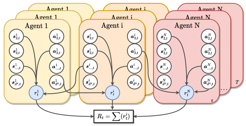
Figure 1: The graphic representation of the causal structure within the MACCA framework. The nodes and edges represent the causal relationships among various environmental variables, i.e., different dimensions of these variables for each agent within the team reward Multi-agent MDP context. These dimensions include the different dimensions of the state $s^{i}_{\cdots,t}$, action $a^{i}_{\cdots,t}$, individual reward $r^{i}_{t}$ for agent $i$, and the team reward $R_{t}$. The individual reward $r^{i}_{t}$ (shown with blue filling) is unobservable, and the aggregation of $r^{i}_{t}$ equals ${R}_{t}$.

In this paper, we propose a new framework, namely Multi-Agent Causal Credit Assignment (MACCA), to address credit assignment in an offline MARL setting. MACCA equates the importance of the credit assignment and how the agent makes the contribution by causal modeling. MACCA first models the generation of individual rewards and team reward from the causal perspective, and construct a graphical representation, as shown in Figure 1, over the involved environment variables, including all the dimensions of states and actions of all agents, the individual rewards and the team rewards. Our method treats team reward as the causal effect of all the individual rewards and provides a way to recover the underlying parametric model, supported by the theoretical evidence of identifiability. In this way, MACCA offers the ability to distinguish the credit of each agent and gain insights into how their states and actions contribute to the individual rewards and further to the team reward. This is achieved through a learned parameterized generative model that decomposes the team reward into individual rewards. The causal structure within the generative process further enhances our understanding by providing insights into the specific contributions of each agent. With the support of theoretical identifiability, we identify the unknown causal structure and individual reward function in such a causal generative process. Additionally, our method offers a clear explanation for actions and states leading to individual rewards, promoting policy optimization and invariance. This clarity enhances agent behavior comprehension and aids in refining policies. The inherent modularity of MACCA ensures its compatibility with a range of policy learning methods, positioning it as a versatile and promising MARL solution for various real-world contexts.

We summarize the main contributions of this paper as follows. First, we reformulate team reward decomposition by introducing a Dynamic Bayesian Network (DBN) to describe the causal relationship among states, actions, individual rewards, and team reward. We provide theoretical evidence of identifiability to learn the causal structure and function within the generation of individual rewards and team rewards. Second, our proposed method can recover the parameterized underlying generative process. Lastly, the empirical results on both discrete and continuous action settings, all three environments, demonstrate that MACCA outperforms current state-of-the-art methods in solving the credit assignment problem caused by team rewards.

2 Related Work

In this section, we review the close-related topics, i.e., Offline MARL and Multi-agent Credit Assignment and Causal Reinforcement Learning.

Offline MARL. Recent research (Pan et al., 2022; Kostrikov et al., 2022; Jiang & Lu, 2021) efforts have delved into offline MARL, identified and addressed some of the issues inherited from offline single-agent RL (Agarwal et al., 2020; Yu et al., 2020; Yang et al., 2022; Wang et al., 2023). For instance, ICQ (Kostrikov et al., 2022) focuses on the vulnerability of multi-agent systems to extrapolation errors, while MABCQ (Jiang & Lu, 2021) examines the problem of mismatched transition distributions in fully decentralized offline MARL. However, these studies all assume using a global state and evaluate the action of the agents relying on the team rewards. Other approaches (Tseng et al., 2022) have a long term progress in online fine-tuning for offline MARL training but have not taken into account the learning slowdown caused by credits of agents to the entire team. For the learning framework, the two most popular recent paradigms are Centralized Training with Decentralized Execution (CTDE) and Independent Learning (IL). Recent research (de Witt et al., 2020; Lyu et al., 2021) shows the benefits of decentralized paradigms, which lead to more robust performance compared to a centralized value function.

Multi-agent Credit Assignment. Multi-agent Credit Assignment is the study to decompose the team reward to each individual agent in the cooperative multi-agent environments (Chang et al., 2003; Du et al., 2019; Chen et al., 2023). Recent works (Sunehag et al., 2018; Foerster et al., 2018; Wang et al., 2020; Rashid et al., 2020; Li et al., 2021) focus on value function decompose under online MARL manner. For instance, COMA (Foerster et al., 2018) is a representative method that uses a centralized critic to estimate the counterfactual advantage of an agent action, which is an on-policy algorithm. This means it requires the corresponding data distribution and samples consistent with the current policy for updates. However, in an offline setting, agents are limited to previously collected data and can’t interact with the environment. This data, often from varying behavioral policies, might not align with the current policy. Therefore, COMA cannot be directly extended to the offline setting without changing its on-policy features (Levine et al., 2020). In online off-policy settings, state-of-the-art credit assignment algorithms such as SHAQ (Wang et al., 2022a) and SQDDPG (Wang et al., 2020) utilize an agent’s approximate Shapley value for credit assignment. In the experiment section, we conduct a comparative analysis with these methods, and the results for MACCA demonstrate superior performance. Note that we focus on explicitly decomposing the team reward into individual rewards in an offline setting under the casual structure we learned, and these decomposed rewards will be used to reconstruct the offline prioritized dataset and further the policy learning phase.

Causal Reinforcement Learning. Plenty of work explores solving diverse RL problems with causal structure. Most conduct research on the transfer ability of RL agents. For instance, Huang et al. (2021) learn factored representation and an individual change factor for different domains, and Feng et al. (2022) extend it to cope with non-stationary changes. More recently, Wang et al. (2022b) and Pitis et al. (2022) remove unnecessary dependencies between states and actions variables in the causal dynamics model to improve the generalizing capability in the unseen state, Hu et al. (2023) use causal structure to discover the dependencies between actions and terms of the reward function in order to exploit these dependencies in a policy learning procedure that reduces gradient variance, Zhang et al. (2023) using the causal structure to solve the single agent temporal credit assignment problem. Also, causal modeling is introduced to multi-agent task (Grimbly et al., 2021; Jaques et al., 2019), model-based RL (Zhang & Bareinboim, 2016), imitation learning (Zhang et al., 2020) and so on. However, most of the previous work does not consider the offline manner and check out the contribution of which dimension of joint state and reward to the individual reward. Compared with the previous work, we investigate the causes for the generation of individual rewards from team rewards in order to help the decentralized policy learning.

3 Preliminaries

In this section, we review the widely-used MARL training framework, the Decentralized Partially Observable Markov Decision Process, and briefly introduce Offline MARL.

Decentralized Partially Observable Markov Decision Process (Dec-POMDP). Dec-POMDP is a widely used model for coordination among multiple agents, and it is defined by a tuple ${\mathcal{M}}=\left<N,\mathcal{S},\mathcal{A},\mathcal{P},\mathcal{R},\mathcal{O},\Omega,\gamma\right>$. In this tuple, $N$ represents the number of agents, $\mathcal{S}$ and $\mathcal{A}$ denote the state and action spaces, respectively. The state transition function $\mathcal{P}:\mathcal{S}\times\mathcal{A}\rightarrow[0,1]$ specifies the probability of transitioning to a new state given the current state and action. Each agent receives the team reward $R_{t}$ at time step $t$ based on the team reward function $\mathcal{R}:\mathcal{S}\times\mathcal{A}\rightarrow\mathbb{R}$ and an individual observation $o^{i}$ from the observation function $\mathcal{O}(s,i):\mathcal{S}\times\mathcal{A}\rightarrow\Omega$, where $\Omega$ denotes the joint observation space. The objective for each agent is to find an optimal policy ${\pi}^{*}$ that maximizes the team discounted return, which is denoted as ${\pi}^{*}=\operatorname*{arg\,max}_{\pi}\mathbb{E}[\sum_{t=0}^{\infty}\sum_{i}^{N}\gamma^{t}{\mathcal{R}}(\bm{s}_{t},\bm{a}_{t})]$, where $\gamma$ represents the discount factor. The Dec-POMDP model is flexible and can be used in a wide range of multi-agent scenarios, making it a popular choice for coordination among multiple agents.

Offline MARL. Under offline setting, we consider a MARL scenario where agents sample from a fixed dataset $\mathcal{D}=\{s^{i}_{t},o^{i}_{t},a^{i}_{t},R_{t},{s^{i}_{t}}^{\prime},{o^{i}_{t}}^{\prime}\}$. This dataset is generated from the behavior policy $\pi_{b}$ without any interaction with the environments, meaning that the dataset is pre-collected offline. Here, $s^{i}_{t}$, $o^{i}_{t}$ and $a^{i}_{t}$ represent the state, observation and action of agent $i$ at time $t$, while $R_{t}$ is the team reward received at time $t$, and ${s^{i}_{t}}^{\prime}$, ${o^{i}_{t}}^{\prime}$ represents the next state and observation of agent $i$.

4 Offline MARL with Causal Credit Assignment

Credit assignment plays a crucial role in facilitating the effective learning of policies in offline cooperative scenarios. In this section, we begin with presenting the underlying generative process within the offline MARL scenario, which serves as the foundation of our methods. Then, we show how to recover the underlying generative process and perform policy learning with the assigned individual rewards.

In our method as shown in Figure 2, there are two main components, including causal model $\psi_{\text{m}}$ and policy model $\psi_{\pi}$. The overall objective contains two parts, $L_{\text{m}}$ for model estimation and $J_{\pi}$ for offline policy learning. Therefore, we minimize the following loss term:

$$L_{\text{MACCA}}=L_{\text{m}}+J_{\pi},$$ (1)

where $J_{\pi}$ depends on the applied offline RL algorithms ($J_{\pi}^{\text{CQR}}$ , $J_{\pi}^{\text{OMAR}}$ or $J_{\pi}^{\text{ICQ}}$ in this paper.)

4.1 Underlying Generative Process in MARL

As a foundation of our method, we introduce a Dynamic Bayesian Network (DBN) (Murphy, 2002) to characterize the underlying generative process, leading to a natural interpretation of the explicit contribution of each dimension of state and action towards the individual rewards.

We denote the $\mathcal{G}$ as the DBN to represent the causal structure between the states, actions, individual rewards, and team reward as shown in Figure 1, which is constructed over a finite number of random variables as $({s^{i}_{1,t},\cdots,s^{i}_{d_{s}^{i},t}},{a^{i}_{1,t},\cdots,a^{i}_{d^{i}_{a},t}},r^{i}_{t},R_{t})^{N,T}_{i,t=1}$, where the $d^{i}_{{s}}$ and $d^{i}_{a}$ correspond to the dimensions of the state and action of agent $i$ respectively. $R_{t}$ is the observed team reward at time step $t$. $r^{i}_{t}$ is the unobserved individual reward at time step $t$. $T$ is the maximum episode length of the environment. Then, the underlying generative process is denoted as:

$$\begin{cases}{r^{i}_{t}}=f(\bm{c}^{i,\bm{s}\rightarrow r}\odot\bm{s}_{t},\bm{c}^{i,\bm{a}\rightarrow r}\odot\bm{a}_{t},i,{\epsilon}_{i,t})\\ {{R}_{t}}=\sum({{r}^{1}_{t}},\cdots{{r}^{N}_{t}})\end{cases}$$ (2)

where, the $\bm{s}_{t}=\{s^{1}_{1,t},...,s^{1}_{d^{1}_{s},t},...,s^{N}_{1,t}....,s^{N}_{d^{N}_{s},t}\}$ and $\bm{a}_{t}=\{a^{1}_{1,t},...,a^{1}_{d^{1}_{a},t},...,a^{N}_{1,t}....,a^{N}_{d^{N}_{a},t}\}$ is the joint state and action of all agents at time step $t$. Define $D_{\bm{s}}$ and $D_{\bm{a}}$ as the numbers of dimensions of joint state and joint action, where $D_{\bm{s}}=\sum_{i=1}^{N}d^{i}_{\bm{s}}$ and $D_{\bm{a}}=\sum_{i=1}^{N}d^{i}_{\bm{a}}$. The $\odot$ is the element-wise product, the $f$ is the unknown non-linear individual reward function, and the ${\epsilon}_{r,i,t}$ is the i.i.d noise. The masks $\bm{c}^{i,\bm{s}\rightarrow r}\in{\{0,1\}}^{D_{\bm{s}}}$ and $\bm{c}^{i,\bm{a}\rightarrow r}\in{\{0,1\}}^{D_{\bm{a}}}$ are vectors and can be dynamic or static depending on the specific requirements from learning phase, in which control if a specific dimension of the state $\bm{s}$ and action $\bm{a}$ impact the individual reward $r^{i}_{t}$, separately. Define ${c}^{j,\bm{s}\rightarrow r}(k)$ as the $k$-th element in the vector ${c}^{j,\bm{s}\rightarrow r}$. For instance, if there is an edge from the $k$-th dimension of $\bm{s}$ to the agent $j$’s individual reward $r^{j}_{t}$ in $\mathcal{G}$, then the ${c}^{j,\bm{s}\rightarrow r}(k)$ is $1$.

Proposition 1 (Identifiability of Causal Structure and Individual Reward Function).

Suppose the joint state $\bm{s}_{t}$, joint action $\bm{a}_{t}$, team reward $R_{t}$ are observable while the individual $r^{i}_{t}$ for each agent are unobserved, and they are from the Dec-POMDP, as described in Eq 2. Then under the Markov condition and faithfulness assumption (refer to Appendix A), given the current time step’s team reward $R_{t}$, all the masks $\bm{c}^{i,\bm{s}\rightarrow r}$, $\bm{c}^{i,\bm{a}\rightarrow r}$, as well as the function $f$ are identifiable.

The proposition 1 demonstrates that we can identify causal representations from the joint action and state, which serve as the causal parents of the individual reward function we want to fit. This allows us to determine which agent should be responsible for which dimension and thus generate the corresponding individual reward function for each agent. The objective for each agent changes to maximize the sum of individual rewards over an infinite horizon. The proof is in Appendix B.

Figure 2: The illustration of the MACCA method. The offline data generation process begins on the left side, where data is recorded from the environment. MACCA then constructs a causal model consisting of a DBN represented in grey and an individual reward predictor depicted in blue. The DBN is used to sample scales from each agent, denoted as $c_{t}^{i,\cdot\rightarrow\cdot}$ and highlighted in green. Meanwhile, the individual reward predictor takes the joint state, action, and these masks as input to generate the individual reward estimate $\hat{r}^{i}_{t}$. During the policy learning phase, each agent utilizes their observation and individual reward estimate as inputs, which are then passed through their respective policy network to generate the next-state actions.

4.2 Causal Model Learning

In this section, we delve into identifying the unknown causal structure and reward function within the graph $\mathcal{G}$. This is achieved using the causal structure predictor $\psi_{g}$, and the individual reward predictor $\psi_{r}$. The set $\psi_{g}=\{\psi_{g}^{\bm{s}\rightarrow r},\psi_{g}^{\bm{a}\rightarrow r}\}$ is to learn the causal structure. Specifically, $\psi_{g}^{\bm{s}\rightarrow r}$ and $\psi_{g}^{i,\bm{a}\rightarrow r}$ are employed to predict the presence of edges in the masks described by Eq 2. We have

$$\begin{array}[]{l}{\hat{\bm{c}}_{t}^{i,\bm{s}\rightarrow r}=\psi_{g}^{\bm{s}\rightarrow r}(\bm{s}_{t},\bm{a}_{t},i)},{\hat{\bm{c}}_{t}^{i,\bm{a}\rightarrow r}=\psi_{g}^{\bm{a}\rightarrow r}(\bm{s}_{t},\bm{a}_{t},i)},\end{array}$$ (3)

where, $\hat{\bm{c}}_{t}^{i,\bm{s}\rightarrow r}$ and $\hat{\bm{c}}_{t}^{i,\bm{a}\rightarrow r}$ are the predicted masks for agent $i$ at timestep $t$. We generate masks at each time step since we consider the inherent complexity of the multi-agent scenario, which has high dimensionality and the dynamic nature of the causal relationships that can evolve over time. Thus, we adopt $\psi_{g}^{\bm{s}\rightarrow r}$ and $\psi_{g}^{\bm{a}\rightarrow r}$ to generate mask estimation at each time step $t$, within the joint state and joint action and agent id as the input. This dynamic mask adaptation facilitates more accurate causal modeling. To further validate this estimation, we have conducted ablation experiments at Section 5.3.

$\psi_{r}$ is used for approximating the function $f$, and is constructed by stacked fully-connection layers. To recover the underlying generative process, i.e., to optimize $\psi_{r}$, we minimize the following objective:

$$\begin{array}[]{l}L_{\text{m}}=\mathbb{E}_{\bm{s}_{t},\bm{a}_{t},R_{t}\sim\mathcal{D}}[R_{t}-\sum_{i=1}^{N}{\psi_{r}}(\hat{\bm{c}}_{t}^{i,\bm{s}\rightarrow r},\hat{\bm{c}}_{t}^{i,\bm{a}\rightarrow r},\bm{s}_{t},\bm{a}_{t},i)]^{2}+L_{\text{reg}}.\end{array}$$ (4)

The $L_{\text{reg}}$ serves as an L1 regularization, akin to the purpose delineated in Zhang & Spirtes (2011). Its primary objective is to clear redundant features during training, reduce the number of features that a given depends on, and use the coefficients of other features completely set to zero, which fosters model interpretability and mitigates the risk of overfitting. And it defines as:

$$\begin{array}[]{l}L_{\text{reg}}=\lambda_{1}\sum_{i=1}^{N}\|\hat{\bm{c}}_{t}^{i,\bm{s}\rightarrow r}\|_{1}+\lambda_{2}\sum_{i=1}^{N}\|\hat{\bm{c}}_{t}^{i,\bm{a}\rightarrow r}\|_{1},\\ \end{array}$$ (5)

where $\lambda_{(\cdot)}$ are hyper-parameters. For more details, please refer to Appendix D.

4.3 Policy Learning with Assigned Individual Rewards.

For policy learning, we use the redistributed individual rewards $\tilde{r}^{i}_{t}$ to replace the observed team reward $R_{t}$. Then, we carry out the policy optimizing over the offline dataset $\mathcal{D}$.

Individual Rewards Assignment.

We first assign individual rewards for each agent’s state-action-id tuple $\langle\bm{s}_{t},\bm{a}_{t},i\rangle$ in the samples used for policy learning. During such an inference phase of individual rewards predictor, we first utilize a hyper-parameter, $h$, as a threshold to determine the existence of the inference phase. Then the values of $\hat{\bm{c}}_{t}^{i,\bm{s}\rightarrow r}$ and $\hat{\bm{c}}_{t}^{i,\bm{a}\rightarrow r}$ are set to be zero while their L1-norms are less than $h$. Then, we assign the individual reward for each agent as:

$$\hat{r}^{i}_{t}={\psi_{r}}(\bm{s}_{t},\bm{a}_{t},\hat{\bm{c}}_{t}^{i,\bm{s}\rightarrow r},\hat{\bm{c}}_{t}^{i,\bm{a}\rightarrow r},i).$$ (6)

Table 1: Average Normalized Score of MPE task with Team Reward

	OMAR	I-CQL	MA-ICQ	MACCA-CQL	MACCA-OMAR	MACCA-ICQ
Exp(CN)	44.7 $\pm$ 46.6	33.6 $\pm$ 22.9	45.0 $\pm$ 23.1	85.4 $\pm$ 8.1	111.7 $\pm$ 4.3	90.4 $\pm$ 5.1
Exp(PP)	99.9 $\pm$ 14.2	63.4 $\pm$ 38.6	87.0 $\pm$ 12.3	94.9 $\pm$ 27.9	111.0 $\pm$ 21.5	114.4 $\pm$ 25.1
Exp(WORLD)	98.7 $\pm$ 18.7	54.4 $\pm$ 17.3	43.2 $\pm$ 15.7	89.3 $\pm$ 14.8	107.4 $\pm$ 11.0	93.2 $\pm$ 12.0
Med(CN)	49.6 $\pm$ 14.9	19.7 $\pm$ 8.7	30.8 $\pm$ 7.3	45.0 $\pm$ 8.8	67.9 $\pm$ 16.9	70.3$\pm$ 10.4
Med(PP)	57.4 $\pm$ 13.9	50.0 $\pm$ 15.6	59.4 $\pm$ 11.1	61.1 $\pm$ 27.1	87.1 $\pm$ 12.2	77.4 $\pm$ 10.5
Med(WORLD)	33.4 $\pm$ 12.8	25.7 $\pm$ 21.3	35.6 $\pm$ 6.0	54.7 $\pm$ 11.0	63.6 $\pm$ 8.7	55.1 $\pm$ 3.5
Med-R(CN)	26.8 $\pm$ 15.2	10.8 $\pm$ 7.7	22.4 $\pm$ 9.3	15.9 $\pm$ 11.2	33.2 $\pm$ 12.6	28.6 $\pm$ 5.6
Med-R(PP)	56.3 $\pm$ 16.6	18.3 $\pm$ 9.5	44.2 $\pm$ 4.5	32.5 $\pm$ 15.1	69.0 $\pm$ 19.3	64.3 $\pm$ 7.8
Med-R(WORLD)	28.9 $\pm$ 17.2	4.5 $\pm$ 10.1	10.7 $\pm$ 2.8	34.8 $\pm$ 16.7	50.9 $\pm$ 14.2	39.9 $\pm$ 13.4
Rand(CN)	22.9 $\pm$ 10.4	12.4 $\pm$ 9.1	6.0 $\pm$ 3.1	22.2 $\pm$ 4.6	32.8 $\pm$ 9.5	28.13 $\pm$ 4.6
Rand(PP)	12.0 $\pm$ 5.2	5.5 $\pm$ 2.8	15.6 $\pm$ 3.4	14.7 $\pm$ 6.7	20.9 $\pm$ 8.3	30.3 $\pm$ 5.4
Rand(WORLD)	6.2 $\pm$ 6.7	0.1 $\pm$ 4.5	0.6 $\pm$ 2.4	8.7 $\pm$ 3.3	15.8 $\pm$ 6.1	10.1 $\pm$ 6.6

Offline Policy Learning.

The process of individual reward assignment is flexible and is able to be inserted into any policy training algorithm. We now describe three practical offline MARL methods, MACCA-CQL, MACCA-OMAR and MACCA-ICQ. In all those methods, they use Q-Value to guide policy learning, for each agent who estimates the $Q^{i}(o^{i},a^{i})=E_{\pi}[\sum_{t=0}^{\infty}\gamma^{t}R_{t}]$ with the Bellman backup operator, we then replace the team reward by learned individual reward $\hat{r}^{i}_{t}$ as $\hat{Q}^{i}(o^{i},a^{i})=E_{\pi}[\sum_{t=0}^{\infty}\gamma^{t}\hat{r}^{i}_{t}]$, then in the policy improvement step, MACCA-CQL trains actors by minimizing:

$$J_{\pi}^{\text{CQL}}=\mathbb{E}_{\mathcal{D}}[(\hat{Q}^{i}(o^{i},a^{i})-y^{i})^{2}]+\alpha\mathbb{E}_{\mathcal{D}}[\log\sum_{a^{i}}\exp(\hat{Q}^{i}(o^{i},a^{i}))-\mathbb{E}_{a^{i}\sim\hat{\pi}^{i}_{\beta}}[\hat{Q}^{i}(o^{i},a^{i})]],$$ (7)

where, $y^{i}=\hat{r}^{i}_{t}+\gamma\min_{k=1,2}\bar{Q}^{i,k}({o^{i}}^{\prime},\bar{\pi}^{i}({o^{i}}^{\prime}))$ from Fujimoto et al. (2018) to minimize the temporal difference error, $\bar{Q}^{i}$ represents the target $\hat{Q}$ for the agent $i$, $\alpha$ is the regularization coefficient, $\hat{\pi}_{\beta^{i}}$ is the empirical behavior policy of agent $i$ in the dataset. Similarly, MACCA-OMAR updates actors by minimizing:

$$J_{\pi}^{\text{OMAR}}=-\mathbb{E}_{\mathcal{D}}[(1-\tau)\hat{Q}^{i}(o^{i},\pi^{i}(o^{i}))-\tau(\pi^{i}(o^{i})-\hat{a}_{i})^{2}],$$ (8)

where $\hat{a}_{i}$ is the action provided by the zeroth-order optimizer and $\tau\in[0,1]$ denotes the coefficient. For the MACCA-ICQ, it updates actors by minimizing:

$$J_{\pi}^{\mathrm{ICQ}}=\mathbb{E}_{\mathcal{D}}[L_{2}^{\tau}(\hat{r}(s,a)+\gamma\bar{Q}^{i}(o^{i^{\prime}},a^{i^{\prime}})-\hat{Q}^{i}(o^{i},a^{i}))],$$ (9)

where $L_{2}^{\tau}$ is the squared loss based on expectile regression and the $\gamma$ is the discount factor, which determines the present value of future rewards. As MACCA uses individual reward to replace the team reward, we do not directly decompose value function, unlike the prior offline MARL methods (Foerster et al., 2018; Wang et al., 2020, 2022a), thus we do not require fitting an additional advantage value or Q-value estimator, simplifying our method.

5 Experiments

Based on the above, our methods include MACCA-OMAR, MACCA-CQL and MACCA-ICQ. For baselines, we compare with both CTDE and independent learning paradigm methods, including I-CQL (Yang et al., 2021): conservative Q-learning in independent paradigm, OMAR (Pan et al., 2022): based on I-CQL, but learning better coordination actions among agents using zeroth-order optimization, MA-ICQ (Kumar et al., 2020): Implicit constraint Q-learning within CTDE paradigm, SHAQ (Wang et al., 2022a) and SQDDPG (Wang et al., 2020): variants of credit assignment method using Shapley value, which are the SOTA on the online multi-agent RL, SHAQ-CQL: In pursuit of a more fair comparison, we integrated CQL with SHAQ, which adopts the architectural framework of SHAQ while using CQL in the estimations of agents’ Q-values and the target Q-values, QMIX-CQL: conservative Q-learning within CTDE paradigm, following QMIX structure to calculate the $Q^{tot}$ using a mixing layer, which is similar to the MA-ICQ framework. We evaluate those performance in two environments: Multi-agent Particle Environments (MPE) (Lowe et al., 2017)and StarCraft Micromanagement Challenges (SMAC) (Samvelyan et al., 2019). Through these comparative evaluations, we want to highlight the relative effectiveness and superiority of the MACCA approach. Furthermore, we conduct three ablations to investigate the interpretability and efficiency of our method. For detailed information about the environments, please refer to Appendix C.

5.1 General Implementation

Offline Dataset. Following the approach outlined in Justin et al. (2020) and Pan et al. (2022), we classify the offline datasets in all environments into four types: Random, generated by random initialization. Medium-Reply, collected from the replay buffer until the policy reaches medium performance. Medium and Expert, collected from partially trained to moderately performing policies and fully trained policies, respectively. The difference between our setup and Pan et al. (2022) is that we hide individual rewards during training and store the sum of these individual rewards in the dataset as the team reward. By creating these different datasets, we aim to explore how different data qualities affect algorithms. For MPE, we adopt the normalized score as a metric to assess performance. The normalized score is calculated by $100\times(S-S_{\text{random}})/(S_{\text{expert}}-S_{\text{random}})$ following by  Justin et al. (2020), where the $S,S_{\text{random}},S_{\text{expert}}$ are the evaluation return from the current policy, random set behavior policy, expert set behavior policy respectively.

5.2 Main Results

Multi-agent Particle Environment (MPE).

We evaluate our method in three distinct environments: Cooperative Navigation (CN), Prey-and-Predator (PP), and Simple-World (WORLD). In the CN environment, three agents aim to reach targets. Observations include position, velocity, and displacements to targets and other agents. Actions are continuous in x and y. Rewards are based on distance to targets, with collision penalties. In the PP environment, three predators chase a random prey. Their state includes position, velocity, and relative displacements. Rewards are based on distance to the prey, with bonuses for captures. The WORLD environment has four allies chasing two faster adversaries. As depicted in Table 1, It can be seen that in all maps and different datasets of MPE, MACCA-based shows better performance than the current state-of-the-art technology. And comparing them with their backbone algorithms respectively, they have improved.

Table 2: Averaged win rate of MACCA-based algorithms and baselines in StarCraft II tasks

Map	Dataset	I-CQL	OMAR	MA-ICQ	MACCA-CQL	MACCA-OMAR	MACCA-ICQ
2s3z (Easy)	Expert	0.70±0.09	0.86±0.08	0.80±0.01	0.88±0.07	0.99±0.05	0.95±0.01
	Medium	0.20±0.03	0.17±0.01	0.16±0.07	0.27±0.02	0.55±0.03	0.51±0.03
	Medium-Replay	0.11±0.07	0.35±0.08	0.31±0.04	0.25±0.03	0.53±0.01	0.59±0.04
5m_vs_6m (Hard)	Expert	0.02±0.02	0.44±0.04	0.38±0.05	0.63±0.02	0.73±0.04	0.88±0.01
	Medium	0.01±0.00	0.14±0.02	0.11±0.04	0.19±0.01	0.20±0.04	0.15±0.02
	Medium-Replay	0.12±0.01	0.09±0.04	0.18±0.04	0.15±0.02	0.14±0.01	0.28±0.01
6h_vs_8z (Super Hard)	Expert	0.00±0.00	0.18±0.08	0.04±0.01	0.59±0.01	0.75±0.07	0.60±0.03
	Medium	0.01±0.01	0.12±0.06	0.01±0.01	0.17±0.00	0.20±0.02	0.22±0.04
	Medium-Replay	0.03±0.02	0.01±0.01	0.07±0.04	0.14±0.02	0.22±0.01	0.25±0.05
MMM2 (Super Hard)	Expert	0.08±0.03	0.10±0.01	0.11±0.01	0.60±0.01	0.69±0.01	0.71±0.03
	Medium	0.02±0.01	0.12±0.02	0.08±0.04	0.25±0.07	0.50±0.06	0.59±0.04

StarCraft Micromanagement Challenges (SMAC).

In order to show the performance in the scale scene, we specially selected maps with a large number of agents. To illustrate, the map $2s3z$ needs to control 5 agents, including 2 Stalkers and 3 Zealots, the map 6h_vs_8z needs to control 6 Hydralisks against 8 Zealots, and map MMM2 have 1 Medivac, 2 Marauders and 7 Marines. All experiments will run 3 random seeds and the win rate was recorded, and the corresponding standard was calculated. Table 2 shows the result. For most of the tasks, the MACCA-based method shows state-of-the-art performance compared to their baseline algorithms.

Also, we considered testing online off-policy algorithms in the offline setting. To this end, we introduced several baselines in SMAC for comparison with MACCA, as shown in Table 3. The table below shows the results of the added baselines compared to SMAC tasks. It becomes apparent that when directly applied to the offline setting, online off-policy credit assignment algorithms consistently yield suboptimal performance. Our empirical findings underscore that while SHAQ-CQL indeed exhibits advancements QMIX-CQL, our MACCA-CQL clinches the SOTA performance across all tasks.

Table 3: Compare with online off-policy credit assignment baselines in SMAC

Map	Dataset	SHAQ	SQDDPG	SHAQ-CQL	QMIX-CQL	ICQL	MACCA-CQL
2s3z	Expert	0.10±0.03	0.05±0.01	0.79±0.03	0.73±0.02	0.70±0.09	0.88±0.07
	Medium	0.05±0.03	0.07±0.01	0.24±0.01	0.22±0.03	0.20±0.03	0.27±0.02
5m_vs_6m	Expert	0.02±0.01	0.00±0.00	0.10±0.03	0.03±0.01	0.02±0.02	0.63±0.02
	Medium	0.00±0.00	0.00±0.00	0.06±0.01	0.01±0.01	0.01±0.00	0.19±0.01
6h_vs_8z	Expert	0.00±0.00	0.00±0.00	0.02±0.01	0.00±0.00	0.00±0.00	0.59±0.01
	Medium	0.00±0.00	0.00±0.00	0.04±0.02	0.00±0.00	0.01±0.01	0.17±0.00

5.3 Ablation Studies

The impact of learned causal structure. We varied the value of $\lambda_{1}$ in Eq 5 to control the sparsity of the learned causal structure. Table 4 presents the average cumulative reward and the sparsity of the causal structure during the training process in the MPE-CN environment. The sparsity of the causal structure ${\bm{\hat{c}}}_{t}^{i,\bm{s}\rightarrow r}$, is calculated as $\mathcal{S}_{sr}=\sum_{i=1}^{N}\frac{1}{d^{i}_{s}}\sum_{k=1}^{d^{i}_{s}}{\bm{s}}^{i,\bm{s}\rightarrow r}_{k}$, where ${\bm{s}}^{i,\bm{s}\rightarrow r}_{k}$ represent is the value bigger than the threshold $h$. The results indicate that as $\lambda_{1}$ increases from $0$ to $0.5$, the causal structure becomes more sparse (sparsity $\mathcal{S}_{sr}$ decreases), resulting in less policy improvement. This can be attributed to the fact that MACCA may not have enough states to predict individual rewards, leading to misguided policy learning accurately. Conversely, setting a relatively low $\lambda_{1}$ may result in a denser structure that incorporates redundant dimensions, hindering policy learning. Therefore, achieving a reasonable causal structure for the reward function can improve both the convergence speed and the performance of policy training. We also provide the ablation for $\lambda_{2}$, please refer to Appendix.D.4.

Table 4: The mean and the standard variance of average normalized score, sparsity rate $\mathcal{S}_{sr}$ of ${\bm{\hat{c}}}_{t}^{i,\bm{s}\rightarrow r}$ with diverse $\lambda_{1}$ at different time step $t$ in MPE-CN.

$\lambda_{1}$  $/$ $t$	$1e4$	$3e4$	$5e4$	$1e5$	$2e5$
0	-2.43 ± 8.01(0.98)	-14.87± 7.71(0.90)	-12.356± 5.83(0.81)	9.842± 18.89(0.77)	69.04 ± 19.69(0.72)
0.007	-7.88±5.36(0.94)	13.26±27.14(0.47)	60.18±26.14(0.28)	99.78± 19.50(0.15)	111.65± 4.28(0.13)
0.05	-3.66±12.14(0.90)	3.93±42.06(0.34)	10.04± 45.97(0.17)	23.61± 44.18(0.11)	75.81± 34.48(0.10)
0.5	-12.20±3.87(0.87)	-16.19±5.53(0.24)	-8.84± 7.16(0.11)	16.40± 21.04(0.07)	59.23± 35.29(0.01)

Table 5: Average normalized scores for ground truth individual reward comparison in MPE-CN

	OMAR	MACCA-OMAR
With GT	114.9 $\pm$ 2.4	113.7 $\pm$ 2.3
Without GT	43.7 $\pm$ 46.6	111.7 $\pm$ 4.3

Ground Truth Individual Reward. In the MPE CN expert dataset, we investigate the influence of ground truth individual rewards on agent policy updates. Two scenarios are compared: agents update policies using ground truth individual rewards (GT), and agents primarily rely on team rewards (without GT). Notably, OMAR with GT directly employs individual rewards for policy updates, while MACCA-OMAR with GT utilizes individual rewards as a supervisory signal, replacing team rewards in Eq 4. The results, presented in Table 5, demonstrate that MACCA-OMAR with GT achieves similar performance to OMAR with GT. Although MACCA-OMAR with GT exhibits slightly slower convergence and performance due to the learning of unbiased causal structures and individual reward functions, it overcomes this drawback by incorporating individual rewards as supervisory signals, mitigating the bias associated with relying solely on team rewards. More Importantly, MACCA-OMAR effectively addresses the challenge of exclusive team reward reliance by attaining a more comprehensive understanding of individual credits through the causal structure and individual reward function. These findings demonstrate that while MACCA-OMAR’s performance is slightly lower than that of OMAR under GT, it offers the advantage of mitigating the bias caused by relying solely on team rewards.

Table 6: Average win rate in SMAC 5m_vs_6m map, expert dataset.

	OMAR
Backbone	0.44 $\pm$ 0.04
MACCA (FCG)	0.38 $\pm$ 0.02
MACCA (FG w. $h$ clipping)	0.50 $\pm$ 0.01
MACCA (DG w.o $h$ clipping)	0.66 $\pm$ 0.01
MACCA (DG w. $h$ clipping)	0.73 $\pm$ 0.04

Different Causal Graph Setting. To investigate how various causal graph settings affect the algorithm’s performance, we performed an ablation study using the expert data set from the SMAC 5m_vs_6m map. According to the Table 6, here the FCG stands for using fully connected causal graph as the mask ($\hat{c}_{t}^{i,\cdot\rightarrow r}(k)=1$), the FG is to learn a fixed graph without time variants ($\hat{c}^{i,\cdot\rightarrow r}$, without timestep), DCG is to learn a dynamic causal graph ($\hat{c}_{t}^{i,\cdot\rightarrow r}$). The $h$ clipping means using hyper-parameter threshold $h$ to filter the causal mask. Utilizing a fully connected causal graph (FCG) indicates that all states and actions directly influence the reward, resulting in suboptimal performance. This indicates an inability in the current setting to differentiate the individual contributions of agents to the collective reward. While the performance of learning a mask without time variants (FG) shows a marginal improvement over the baseline, the enhancement remains minimal. This can be attributed to the inherent challenges in directly learning a comprehensive multi-agent causal graph, especially given the intricacies of the environment. Similarly, the efficacy of a learned causal graph without threshold clipping (i.e., w.o $h$ clipping) is slightly superior to the baseline but doesn’t match the performance of DG with $h$ clipping. In real-world implementations and when working with finite datasets, the model often finds it challenging to ensure edge weights converge precisely to zero. Even when sparsity loss and normalization are introduced, threshold clipping remains indispensable. Such an approach aligns with established practices in causal structure discovery with continuous optimization, as evidenced by  Zheng et al. (2018) and Ng et al. (2020).

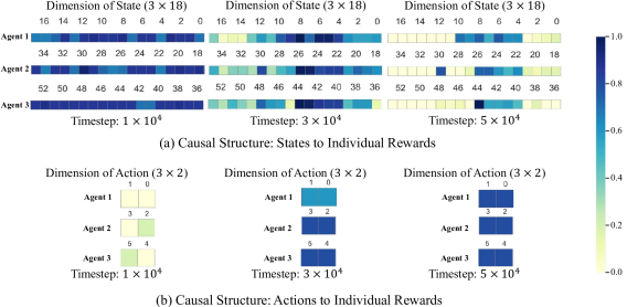
Figure 3: The figure visualizes the causal structure, showing the probability of causal edges from blue (high probability) to yellow (low probability). (a) represents the causal structure $\hat{c}_{t}^{i,s\rightarrow r}$ between the state of all agents (18 dimensions for each agent, 54 dimensions for joint state ) and the individual reward (1 dimension for each agent). (b) represents the causal structure $\hat{c}_{t}^{i,a\rightarrow r}$ between the action of each agent (2 dimensions for each agent, six dimensions for joint action) and the individual reward (1 dimension for each agent).

Visualization of Causal Structure. In Figure 3, we present visualizations of two significant causal structures within the CN environment of MPE. To facilitate the observation of the causal structure learning process, we initialize S2R as a normalized random number close to 1 and A2R as a normalized random number close to 0. As time progresses, we observe that the causal structure $\hat{c}_{t}^{i,s\rightarrow r}$ transitions its focus from considering all dimensions of the agent state to primarily emphasizing the 4th to 10th dimensions of each agent. By analyzing the state output of the environment, we determine that each agent’s state comprises 18 dimensions. Specifically, dimensions 0-4 represent the agent’s velocity and position on the x and y axes, dimensions 4-9 capture the distance between the agent and three distinct landmarks on the x and y axes, dimensions 10-13 reflect the distances between the agent and other agents and dimensions 14-17 are related to communication, although not applicable in this experiment and thus considered as irrelevant. Variables 4-9 and 10-13 are intuitively linked to individual rewards, aligning with the convergence direction of MACCA. Regarding the causal structure $\hat{c}_{t}^{i,a\rightarrow r}$, as each agent’s actions involve continuous motion without extraneous variables, it converges to relevant states that contribute to individual credits for the team reward. The experimental results demonstrate that MACCA exhibits rapid convergence, facilitating the learning of interpretable causal structures within short time steps. Therefore, our findings support the interpretability of the causal structure and its ability to provide a clear understanding of the relationships between variables.

6 Conclusion

In conclusion, MACCA emerges as a valuable solution to the credit assignment problem in offline Multi-agent Reinforcement Learning (MARL), providing an interpretable and modular framework for capturing the intricate interactions within multi-agent systems. By leveraging the inherent causal structure of the system, MACCA allows us to disentangle and identify the specific credits of individual agents to team rewards. This enables us to accurately assign credit and update policies accordingly, leading to enhanced performance compared to different baseline methods. The MACCA framework empowers researchers and practitioners to gain deeper insights into the dynamics of multi-agent systems, facilitating the understanding of the causal factors that drive cooperative behavior and ultimately advancing the capabilities of MARL in a variety of real-world applications.

7 Reproducibility Statement

To promote transparent and accountable research practices, we have prioritized the reproducibility of our method. All experiments conducted in this study adhere to controlled conditions and well-known environments and datasets, with detailed descriptions of the experimental settings available in Section 5 and Appendix C. The implementation specifics for all the baseline methods and our proposed MACCA are thoroughly outlined in Section 4 and Appendix D.

Appendix A Markov and Faithfulness Assumptions

A directed acyclic graph (DAG), $\mathcal{G}=(\bm{V},\bm{E})$, can be deployed to represent a graphical criterion carrying out a set of conditions on the paths, where $\bm{V}$ and $\bm{E}$ denote the set of nodes and the set of directed edges, separately.

Definition 1.

(d-separation (Pearl, 2009)). A set of nodes $\bm{Z}\subseteq\bm{V}$ blocks the path $p$ if and only if (1) $p$ contains a chain $i\rightarrow m\rightarrow j$ or a fork $i\leftarrow m\rightarrow j$ such that the middle node $m$ is in $\bm{Z}$, or (2) $p$ contains a collider $i\rightarrow m\leftarrow j$ such that the middle node $m$ is not in $\bm{Z}$ and such that no descendant of $m$ is in $\bm{Z}$. Let $\bm{X}$, $\bm{Y}$ and $\bm{Z}$ be disjunct sets of nodes. If and only if the set $\bm{Z}$ blocks all paths from one node in $\bm{X}$ to one node in $\bm{Y}$, $\bm{Z}$ is considered to d-separate $\bm{X}$ from $\bm{Y}$, denoting as $(\bm{X}\perp_{d}\bm{Y}\mid\bm{Z})$.

Definition 2.

(Global Markov Condition (Spirtes et al., 2000; Pearl, 2009)). If, for any partition $(\bm{X},\bm{Y},\bm{Z})$, $\bm{X}$ is d-separated from $\bm{Y}$ given $\bm{Z}$, i.e. $\bm{X}\perp_{d}\bm{Y}\mid\bm{Z}$. Then the distribution $P$ over $\bm{V}$ satisfies the global Markov condition on graph $G$, and can be factorizes as, $P(\bm{X},\bm{Y}\mid\bm{Z})=P(\bm{X}\mid\bm{Z})P(\bm{Y}\mid\bm{Z})$. That is, $\bm{X}$ is conditionally independent of $\bm{Y}$ given $\bm{Z}$, writing as $\bm{X}\perp\!\!\!\perp\bm{Y}\mid\bm{Z}$.

Definition 3.

(Faithfulness Assumption (Spirtes et al., 2000; Pearl, 2009)). The variables, which are not entailed by the Markov Condition, are not independent of each other.

Under the above assumptions, we can apply d-separation as a criterion to understand the conditional independencies from a given DAG $G$. That is, for any disjoint subset of nodes $\bm{X},\bm{Y},\bm{Z}\subseteq\bm{V}$, $(\bm{X}\perp\!\!\!\perp\bm{Y}\mid\bm{Z})$ and $\bm{X}\perp_{d}\bm{Y}\mid\bm{Z}$ are the necessary and sufficient condition of each other.

Appendix B Proof of Identifiability

Proposition 1 (Individual Reward Function Identifiability).

Suppose the joint state $\bm{s}_{t}$, joint action $\bm{a}_{t}$, team reward $R_{t}$ are observable while the individual $r^{i}_{t}$ for each agent are unobserved, and they are from the Dec-POMDP, as described in Eq 2. Then, under the Markov condition and faithfulness assumption, given the current time step’s team reward $R_{t}$, all the masks $\bm{c}^{\bm{s}\rightarrow r,i}$, $\bm{c}^{\bm{a}\rightarrow r,i}$, as well as the function $f$ are identifiable.

Assumption

We assume that, $\epsilon_{i,t}$ in Eq 2 are i.i.d additive noise. From the weight-space view of Gaussian Process (Williams & Rasmussen, 2006) and equation.6, equivalently, the causal models for $r^{i}_{t}$ can be represented as follows,

$$r^{i}_{t}=f(\bm{c}_{t}^{i,\bm{s}\rightarrow r}\odot\bm{s}_{t},\bm{c}_{t}^{i,\bm{a}\rightarrow r}\odot\bm{a}_{t},i)+\epsilon_{r,t}={W_{f}}^{T}\phi_{r}(\bm{s}_{t},\bm{a}_{t},i)+\epsilon_{i,t}$$ (A1)

where $\forall i\in[1,N]$, and $\phi_{r}$ denote basis function sets.

As $\bm{s}_{t}=\{s^{1}_{1,t},...,s^{1}_{d^{1}_{s},t},...,s^{N}_{1,t}....,s^{N}_{d^{N}_{s},t}\}$ and $\bm{a}_{t}=\{a^{1}_{1,t},...,a^{1}_{d^{1}_{a},t},...,a^{N}_{1,t}....,a^{N}_{d^{N}_{a},t}\}$. We denote the variable set in the system by $\bm{V}=\{\bm{V}_{0},...,\bm{V}_{T}\}$, where $\bm{V}_{t}=\bm{s}_{t}\cup\bm{a}_{t}\cup R_{t}$, and the variables form a Bayesian network $\mathcal{G}$. Following AdaRL (Huang et al., 2021), there are possible edges only from $\bm{s}^{i}_{k,t}\in\bm{s}_{t}$ to $r^{i}_{t}$, and from $\bm{a}^{i}_{j,t}\in\bm{a}_{t}$ to $r^{i}_{t}$ in $\mathcal{G}$, where $k,j$ are dimension index in $[1,...,d^{N}_{s}]$ and $[1,...,d^{N}_{a}]$ respectively. In particular, the $r^{i}_{t}$ are unobserved, while $R_{t}=\sum_{i=1}^{N}r^{i}_{t}$ is observed. Thus, there are deterministic edges from each $r^{i}_{t}$ to $R_{t}$.

Proof

We aim to prove that, given the team reward $R_{t}$, and the $\bm{c}^{i,\bm{s}\rightarrow r}$, $\bm{c}^{i,\bm{a}\rightarrow r}$ and $r^{i}_{t}$ are identifiable. Following the above assumption, we can rewrite the Eq 2 to the following,

$$R_{t} =\sum\limits_{i=1}^{N}r^{i}_{t}$$ (A2)

$$=\sum\limits_{i=1}^{N}{\left[{W_{f}}^{T}\phi_{r}(\bm{s}_{t},\bm{a}_{t},i)+\epsilon_{i,t}\right]}$$

$$={W_{f}}^{T}\sum\limits_{i=1}^{N}{\phi_{r}(\bm{s}_{t},\bm{a}_{t},i)}+\sum\limits_{i=1}^{N}\epsilon_{i,t}.$$

For simplicity, we replace the components in Eq A2 by,

$$\begin{array}[]{ll}{\Phi_{r,t}}&=\sum\limits_{i=1}^{N}\phi_{r}(\bm{s}_{t},\bm{a}_{t},i),\\ \mathcal{E}_{r,t}&=\sum\limits_{i=1}^{N}\epsilon_{i,t}.\end{array}$$ (A3)

Consequently, we derive the following equation,

$$R_{t}={W_{f}}^{T}\Phi_{r,t}(X_{t})+\mathcal{E}_{r,t},$$ (A4)

where $X_{t}:=[\bm{s}_{t},\bm{a}_{t},i]_{i=1}^{N}$ representing the concatenation of the covariates $\bm{s}_{t}$ , $\bm{a}_{t}$ and $i$, from $i=1$ to $N$.

Then we can obtain a closed-form solution of ${W_{f}}^{T}$ in Eq A4 by modelling the dependencies between the covariates $X_{t}$ and response variables $R_{t}$. One classical approach to finding such a solution involves minimizing the quadratic cost and incorporating a weight-decay regularizer to prevent overfitting. Specifically, we define the cost function as,

$$C(W_{f})=\frac{1}{2}\sum_{X_{t},R_{t}\sim\mathcal{D}}(R_{t}-{W_{f}}^{T}\Phi_{r,t}(X_{t}))^{2}+\frac{1}{2}\lambda\|W_{f}\|^{2}.$$ (A5)

where $X_{t}$ and long-term returns $R_{t}$, which are sampled from the offline dataset $\mathcal{D}$. $\lambda$ is the weight-decay regularization parameter. To find the closed-form solution, we differentiate the cost function with respect to $W_{f}$ and set the derivative to zero:

$$\frac{\partial C(W_{f})}{\partial W_{f}}\rightarrow 0.$$ (A6)

Solving Eq A6 will yield the closed-form solution for ${W_{f}}$, as

$$\begin{array}[]{ll}W_{f}=(\lambda I_{d}+\Phi_{r,t}{\Phi_{r,t}}^{T})^{-1}\Phi_{r,t}R_{t}=\Phi_{r,t}({\Phi_{r,t}}^{T}\Phi_{r,t}+\lambda I_{n})^{-1}R_{t}.\end{array}$$ (A7)

Therefore, $W_{f}$, which indicates the causal structure and strength of the edge, can be identified from the observed data. In summary, given team reward $R_{t}$, the binary masks, $\bm{c}^{i,\bm{s}\rightarrow r}$, $\bm{c}^{i,\bm{a}\rightarrow r}$ and individual $r^{i}_{t}$ are identifiable.

Considering the Markov condition and faithfulness assumption, we can conclude that for any pair of variables $V_{k},V_{j}\in\bm{V}$, $V_{k}$ and $V_{j}$ are not adjacent in the causal graph $\mathcal{G}$ if and only if they are conditionally independent given some subset of $\{V_{l}\mid l\neq k,l\neq j\}$. Additionally, since there are no instantaneous causal relationships and the direction of causality can be determined if an edge exists, the binary structural masks $\bm{c}^{i,\bm{s}\rightarrow r}$ and $\bm{c}^{i,\bm{a}\rightarrow r}$ defined over the set $\bm{V}$ are identifiable with conditional independence relationships (Huang et al., 2022). Consequently, the functions $f$ in Equation 2 are also identifiable.

Appendix C Environments Setting

We adopt the open-source implementations for the multi-agent particle environment (Lowe et al., 2017) and SMAC(Samvelyan et al., 2019). The tasks in the multi-agent particle environments are illustrated in Figures A1(a)-(c). The Cooperative Navigation (CN) task involves 3 agents and 3 landmarks, requiring agents to cooperate in covering the landmarks without collisions. In the Predator-Prey (PP) task, 3 predators collaborate to capture prey that is faster than them. Finally, the WORLD task features 4 slower cooperating agents attempting to catch 2 faster adversaries, with the adversaries aiming to consume food while avoiding capture.

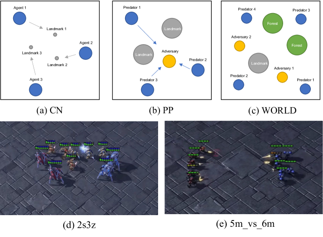
Figure A1: Visualization of different environment in the experiments, (a)-(c): Multi-agent Particle Environments (MPE), (d)-(e): StarCraft Micromanagement Challenges (SMAC)

Datasets. During training, we utilize the team reward as input, while for evaluation purposes, we compare the performance with the ground truth individual reward. As a result, the expert and random scores for the Cooperative Navigation, Predator-Prey and World tasks are as follows: Cooperative Navigation - expert: 516.526, random: 160.042; Predator-Prey - expert: 90.637, random: -2.569; World - expert: 34.661, random: -8.734;

Appendix D Implementations

D.1 Algorithm

Algorithm 1 MACCA: Multi-Agent Causal Credit Assignment

1:  for $\text{training step }t=1\text{ to }T$ do

2:     Sample trajectories from $\mathcal{D}$, save in minibatch $\mathcal{B}$

3:     for $\text{agent }i=1\text{ to }N$ do

4:        Update the team reward $R_{t}$ to $\hat{r}^{i}_{t}$ in $\mathcal{B}$ (Eq 6)

5:        Optimize $\psi_{m}$: $\psi_{m}\leftarrow\psi_{m}-\alpha\nabla_{\psi_{m}}L_{m}$ (Eq 4)

6:     end for

7:     Update policy $\pi$ with minibatch $\mathcal{B}$ (Eq 7, Eq 8 or Eq 9)

8:     Reset $\mathcal{B}\leftarrow\emptyset$

9:  end for

D.2 Model Structure

The parametric generative model $\psi_{\text{m}}$ used in MACCA consists of two parts: $\psi_{\text{g}}$ and $\psi_{\text{r}}$. The function of $\psi_{\text{g}}$ is to predict the causal structure, which determines the relationships between the environment variables. The role of $\psi_{\text{r}}$ is to generate individual rewards based on the joint state and action information. This prediction is achieved through a network architecture that includes three fully-connected layers with an output size of 256, followed by an output layer with a single output. Each hidden layer is activated using the rectified linear unit (ReLU) activation function.

During the training process, the generative model is optimized to learn the causal structure and generate individual rewards that align with the observed team rewards. The model parameters are updated using Adam, to minimize the discrepancy between the predicted sum of individual rewards and the team rewards. The training process involves iteratively adjusting the parameters to improve the accuracy of the predictions.

For a more detailed overview of the training process, including the specific loss functions and optimization algorithms used, please refer to Figure 2. The Figure provides a step-by-step illustration of the training pipeline, helping to visualize the flow of information and the interactions between different components of the generative model.

Table A1: The Common Hyper-parameters.

hyperparameters	value	hyperparameters	value
steps per update	100	optimizer	Adam
batch size	1024	learning rate	$3\times 10^{-4}$
hidden layer dim	64	$\gamma$	0.95
evaluation interval	$1000$	evaluation episodes	10

Table A2: Hyper-parameters for OMAR, CQL and MACCA

	OMAR $\tau$	CQL $\alpha$	MACCA $\lambda_{1}$	MACCA $\lambda_{2}$	MACCA $r_{lr}$	MACCA $h$
Expert	0.9	5.0	7e-3	7e-3	5e-2	0.1
Medium	0.7	0.5	5e-3	5e-3	5e-2	0.1
Medium-Replay	0.7	1.0	5e-3	7e-3	5e-2	0.1
Random	0.99	1.0	1e-7	1e-3	5e-2	0.1

D.3 Hyper-parameters

The neural network used in training is initialized from scratch and optimized using the Adam optimizer with a learning rate of $3\times 10^{-4}$. The policy learning process involves varying initial learning rates based on the specific algorithm, while the hyperparameters for policy learning, including a discount factor of 0.95, are consistent across all tasks.

The training procedure differs across tasks. For MPE, the training duration ranges from 20,000 to 60,000 iterations, with longer training for behavior policies that perform poorly. The number of steps per update is set to 100.

During each training iteration, trajectories are sampled from the offline data, and the generated individual reward is replaced with the team reward for policy updates. The training of $\psi_{\text{cau}}$ is performed concurrently with $\psi_{\text{rew}}$. Validation is conducted after each epoch, and the average metrics are computed using 5 random seeds for reliable evaluation.

The hyperparameters specific to training MACCA models can be found in Table A2. All experiments were conducted on a high-performance computing (HPC) system featuring 128 Intel Xeon processors running at 2.2 GHz, 5 TB of memory, and an Nvidia A100 PCIE-40G GPU. This computational setup ensures efficient processing and reliable performance throughout the experiments.

D.4 Ablation for $\lambda_{2}$

We have conducted ablation experiments on $\lambda_{2}$ and show the results in the Table A3.

Table A3: The mean and the standard variance of average normalized score, sparsity rate $\mathcal{S}_{ar}$ of ${\bm{\hat{c}}}_{t}^{i,\bm{a}\rightarrow r}$ with diverse $\lambda_{2}$ at different time step $t$ in MPE-CN.

$\lambda_{2}$  $/$ $t$	$1e4$	$5e4$	$1e5$	$2e5$
0	17.4 ± 15.2(0.98)	93.1 ± 6.4 (1.0)	105 ± 3.5 (1.0)	107.7 ± 10.2 (1.0)
0.007	19.9 ± 12.4 (0.8	90.2 ± 7.1 (1.0)	108.8 ± 4.0 (1.0)	111.7 ± 4.3(1.0)
0.5	13.3 ± 11.1 (0.68)	100.5 ± 14.0 (0.84)	102.9 ± 16.4 (0.87)	108.4 ± 6.4 (0.98)
5.0	2.3 ± 9.8 (0.0)	-1.3 ± 25.4 (0.34)	70.4 ± 18.0 (0.62)	100.1 ± 7.4 (0.75)

This table shows the mean and the standard variance of the average normalized score with diverse $\lambda_{2}$ in the MPE-CN task. The value in brackets is the sparsity rate $\mathcal{S}_{ar}$ of $\hat{\bm{c}}_{t}^{i,a\rightarrow r}$, whose definition can be found in Section 5.3. For all values of $\lambda_{2}$, the sparsity rate $\mathcal{S}_{ar}$ consistently begins from zero. Over time, there is a discernible increase in $\mathcal{S}_{ar}$, and the convergence speed slows down with the increase of $\lambda_{2}$. This pattern intimates that higher $\lambda_{2}$ values engender a more measured modulation in the causal impact exerted by actions on individual rewards. Furthermore, despite the variation in $\lambda_{2}$ values, the average normalized scores across different $\lambda_{2}$ settings eventually converge towards a similar level.

References

- Agarwal et al. (2020) Rishabh Agarwal, Dale Schuurmans, and Mohammad Norouzi. An optimistic perspective on offline reinforcement learning. In International Conference on Machine Learning, pp. 104–114. PMLR, 2020.
- Chang et al. (2003) Yu-han Chang, Tracey Ho, and Leslie Kaelbling. All learning is local: Multi-agent learning in global reward games. In Advances in Neural Information Processing Systems, volume 16. MIT Press, 2003.
- Chen et al. (2023) Sirui Chen, Zhaowei Zhang, Yali Du, and Yaodong Yang. Stas: Spatial-temporal return decomposition for multi-agent reinforcement learning. In In Proceedings of the AAAI conference on artificial intelligence, 2023.
- de Witt et al. (2020) Christian Schroeder de Witt, Tarun Gupta, Denys Makoviichuk, Viktor Makoviychuk, Philip HS Torr, Mingfei Sun, and Shimon Whiteson. Is independent learning all you need in the starcraft multi-agent challenge? arXiv preprint arXiv:2011.09533, 2020.
- Du et al. (2019) Yali Du, Lei Han, Meng Fang, Ji Liu, Tianhong Dai, and Dacheng Tao. Liir: Learning individual intrinsic reward in multi-agent reinforcement learning. In Advances in Neural Information Processing Systems, volume 32. Curran Associates, Inc., 2019.
- Du et al. (2023) Yali Du, Joel Z Leibo, Usman Islam, Richard Willis, and Peter Sunehag. A review of cooperation in multi-agent learning. arXiv preprint arXiv:2312.05162, 2023.
- Feng et al. (2022) Fan Feng, Biwei Huang, Kun Zhang, and Sara Magliacane. Factored adaptation for non-stationary reinforcement learning. In Advances in Neural Information Processing Systems, volume 35, pp. 31957–31971. Curran Associates, Inc., 2022.
- Foerster et al. (2018) Jakob Foerster, Gregory Farquhar, Triantafyllos Afouras, Nantas Nardelli, and Shimon Whiteson. Counterfactual multi-agent policy gradients. In Proceedings of the AAAI conference on artificial intelligence, volume 32, 2018.
- Fujimoto et al. (2018) Scott Fujimoto, Herke Hoof, and David Meger. Addressing function approximation error in actor-critic methods. In International Conference on Machine Learning, pp. 1587–1596. PMLR, 2018.
- Grimbly et al. (2021) St John Grimbly, Jonathan Shock, and Arnu Pretorius. Causal multi-agent reinforcement learning: Review and open problems. In Cooperative AI Workshop, Advances in Neural Information Processing Systems, 2021.
- Hu et al. (2023) Jiaheng Hu, Peter Stone, and Roberto Martín-Martín. Causal policy gradient for whole-body mobile manipulation. In Robotics: Science and Systems XIX, 2023.
- Huang et al. (2021) Biwei Huang, Fan Feng, Chaochao Lu, Sara Magliacane, and Kun Zhang. Adarl: What, where, and how to adapt in transfer reinforcement learning. In International Conference on Learning Representations, 2021.
- Huang et al. (2022) Biwei Huang, Chaochao Lu, Liu Leqi, José Miguel Hernández-Lobato, Clark Glymour, Bernhard Schölkopf, and Kun Zhang. Action-sufficient state representation learning for control with structural constraints. In International Conference on Machine Learning, pp. 9260–9279. PMLR, 2022.
- Jaques et al. (2019) Natasha Jaques, Angeliki Lazaridou, Edward Hughes, Caglar Gulcehre, Pedro Ortega, DJ Strouse, Joel Z Leibo, and Nando De Freitas. Social influence as intrinsic motivation for multi-agent deep reinforcement learning. In International Conference on Machine Learning, pp. 3040–3049. PMLR, 2019.
- Jiang & Lu (2021) Jiechuan Jiang and Zongqing Lu. Offline decentralized multi-agent reinforcement learning. arXiv preprint arXiv:2108.01832, 2021.
- Justin et al. (2020) Fu Justin, Kumar Aviral, Nachum Ofir, Tucker George, and Levine Sergey. D4rl: Datasets for deep data-driven reinforcement learning. arXiv preprint arXiv:2004.07219, 2020.
- Kostrikov et al. (2022) Ilya Kostrikov, Ashvin Nair, and Sergey Levine. Offline reinforcement learning with implicit q-learning. In International Conference on Learning Representations, 2022.
- Kumar et al. (2020) Aviral Kumar, Aurick Zhou, George Tucker, and Sergey Levine. Conservative q-learning for offline reinforcement learning. In Advances in Neural Information Processing Systems, volume 33, pp. 1179–1191. Curran Associates, Inc., 2020.
- Levine et al. (2020) Sergey Levine, Aviral Kumar, George Tucker, and Justin Fu. Offline reinforcement learning: Tutorial, review, and perspectives on open problems. arXiv preprint arXiv:2005.01643, 2020.
- Li et al. (2021) Jiahui Li, Kun Kuang, Baoxiang Wang, Furui Liu, Long Chen, Fei Wu, and Jun Xiao. Shapley counterfactual credits for multi-agent reinforcement learning. In Proceedings of the 27th ACM SIGKDD Conference on Knowledge Discovery & Data Mining, pp. 934–942, 2021.
- Lowe et al. (2017) Ryan Lowe, Yi Wu, Aviv Tamar, Jean Harb, Pieter Abbeel, and Igor Mordatch. Multi-agent actor-critic for mixed cooperative-competitive environments. In Proceedings of the 31st International Conference on Neural Information Processing Systems, pp. 6382–6393, 2017.
- Lyu et al. (2021) Xueguang Lyu, Yuchen Xiao, Brett Daley, and Christopher Amato. Contrasting centralized and decentralized critics in multi-agent reinforcement learning. In Proceedings of the 20th International Conference on Autonomous Agents and MultiAgent Systems, 2021.
- Murphy (2002) Kevin Patrick Murphy. Dynamic bayesian networks: representation, inference and learning. University of California, Berkeley, 2002.
- Ng et al. (2020) Ignavier Ng, AmirEmad Ghassami, and Kun Zhang. On the role of sparsity and dag constraints for learning linear dags. In Advances in Neural Information Processing Systems, volume 33, pp. 17943–17954. Curran Associates, Inc., 2020.
- Pan et al. (2022) Ling Pan, Longbo Huang, Tengyu Ma, and Huazhe Xu. Plan better amid conservatism: Offline multi-agent reinforcement learning with actor rectification. In International Conference on Machine Learning, pp. 17221–17237. PMLR, 2022.
- Pearl (2009) Judea Pearl. Causality: Models, Reasoning and Inference. Cambridge University Press, 2009.
- Pitis et al. (2022) Silviu Pitis, Elliot Creager, Ajay Mandlekar, and Animesh Garg. Mocoda: Model-based counterfactual data augmentation. In Advances in Neural Information Processing Systems, volume 35, pp. 18143–18156. Curran Associates, Inc., 2022.
- Rashid et al. (2020) Tabish Rashid, Mikayel Samvelyan, Christian Schroeder De Witt, Gregory Farquhar, Jakob Foerster, and Shimon Whiteson. Monotonic value function factorisation for deep multi-agent reinforcement learning. The Journal of Machine Learning Research, 21(1):7234–7284, 2020.
- Samvelyan et al. (2019) Mikayel Samvelyan, Tabish Rashid, Christian Schroeder De Witt, Gregory Farquhar, Nantas Nardelli, Tim GJ Rudner, Chia-Man Hung, Philip HS Torr, Jakob Foerster, and Shimon Whiteson. The starcraft multi-agent challenge. arXiv preprint arXiv:1902.04043, 2019.
- Spirtes et al. (2000) Peter Spirtes, Clark N Glymour, Richard Scheines, and David Heckerman. Causation, prediction, and search. MIT press, 2000.
- Sunehag et al. (2018) Peter Sunehag, Guy Lever, Audrunas Gruslys, Wojciech Marian Czarnecki, Vinicius Zambaldi, Max Jaderberg, Marc Lanctot, Nicolas Sonnerat, Joel Z Leibo, Karl Tuyls, et al. Value-decomposition networks for cooperative multi-agent learning. In Proceedings of the 17th International Conference on Autonomous Agents and MultiAgent Systems, 2018.
- Tseng et al. (2022) Wei-Cheng Tseng, Tsun-Hsuan Johnson Wang, Yen-Chen Lin, and Phillip Isola. Offline multi-agent reinforcement learning with knowledge distillation. In Advances in Neural Information Processing Systems, volume 35, pp. 226–237. Curran Associates, Inc., 2022.
- Wang et al. (2020) Jianhong Wang, Yuan Zhang, Tae-Kyun Kim, and Yunjie Gu. Shapley q-value: A local reward approach to solve global reward games. In Proceedings of the AAAI Conference on Artificial Intelligence, volume 34, pp. 7285–7292, 2020.
- Wang et al. (2022a) Jianhong Wang, Yuan Zhang, Yunjie Gu, and Tae-Kyun Kim. Shaq: Incorporating shapley value theory into multi-agent q-learning. In Advances in Neural Information Processing Systems, volume 35, pp. 5941–5954, 2022a.
- Wang et al. (2023) Mianchu Wang, Rui Yang, Xi Chen, and Meng Fang. Goplan: Goal-conditioned offline reinforcement learning by planning with learned models. In NeurIPS 2023 Workshop on Goal-Conditioned Reinforcement Learning, 2023.
- Wang et al. (2022b) Zizhao Wang, Xuesu Xiao, Zifan Xu, Yuke Zhu, and Peter Stone. Causal dynamics learning for task-independent state abstraction. In International Conference on Machine Learning, pp. 23151–23180, 2022b.
- Williams & Rasmussen (2006) Christopher KI Williams and Carl Edward Rasmussen. Gaussian processes for machine learning, volume 2. MIT press Cambridge, MA, 2006.
- Yang et al. (2022) Rui Yang, Yiming Lu, Wenzhe Li, Hao Sun, Meng Fang, Yali Du, Xiu Li, Lei Han, and Chongjie Zhang. Rethinking goal-conditioned supervised learning and its connection to offline rl. In International Conference on Learning Representations, 2022.
- Yang et al. (2021) Yiqin Yang, Xiaoteng Ma, Chenghao Li, Zewu Zheng, Qiyuan Zhang, Gao Huang, Jun Yang, and Qianchuan Zhao. Believe what you see: Implicit constraint approach for offline multi-agent reinforcement learning. In Advances in Neural Information Processing Systems, volume 34, pp. 10299–10312, 2021.
- Yu et al. (2020) Tianhe Yu, Garrett Thomas, Lantao Yu, Stefano Ermon, James Y Zou, Sergey Levine, Chelsea Finn, and Tengyu Ma. Mopo: Model-based offline policy optimization. In Advances in Neural Information Processing Systems, volume 33, pp. 14129–14142, 2020.
- Zhang & Spirtes (2011) Jiji Zhang and Peter Spirtes. Intervention, determinism, and the causal minimality condition. Synthese, 182(3):335–347, 2011.
- Zhang & Bareinboim (2016) Junzhe Zhang and Elias Bareinboim. Markov decision processes with unobserved confounders: A causal approach. Technical report, Technical report, Technical Report R-23, Purdue AI Lab, 2016.
- Zhang et al. (2020) Junzhe Zhang, Daniel Kumor, and Elias Bareinboim. Causal imitation learning with unobserved confounders. In Advances in Neural Information Processing Systems, volume 33, pp. 12263–12274, 2020.
- Zhang et al. (2023) Yudi Zhang, Yali Du, Biwei Huang, Ziyan Wang, Jun Wang, Meng Fang, and Mykola Pechenizkiy. Interpretable reward redistribution in reinforcement learning: A causal approach. In Advances in Neural Information Processing Systems, 2023.
- Zheng et al. (2018) Xun Zheng, Bryon Aragam, Pradeep K Ravikumar, and Eric P Xing. Dags with no tears: Continuous optimization for structure learning. In Advances in Neural Information Processing Systems, volume 31, 2018.