On the Obtaining Solutions of Nonlinear Differential Equations by Means of the Solutions of Simpler Linear or Nonlinear Differential Equations

Abstract

Transformations are much used to connect complicated nonlinear differential equations to simple equations with known exact solutions. Two examples of this are the Hopf–Cole transformation and the simple equations method. In this article, we follow an idea that is opposite to the idea of Hopf and Cole: we use transformations in order to transform simpler linear or nonlinear differential equations (with known solutions) to more complicated nonlinear differential equations. In such a way, we can obtain numerous exact solutions of nonlinear differential equations. We apply this methodology to the classical parabolic differential equation (the wave equation), to the classical hyperbolic differential equation (the heat equation), and to the classical elliptic differential equation (Laplace equation). In addition, we use the methodology to obtain exact solutions of nonlinear ordinary differential equations by means of the solutions of linear differential equations and by means of the solutions of the nonlinear differential equations of Bernoulli and Riccati. Finally, we demonstrate the capacity of the methodology to lead to exact solutions of nonlinear partial differential equations on the basis of known solutions of other nonlinear partial differential equations. As an example of this, we use the Korteweg–de Vries equation and its solutions. Traveling wave solutions of nonlinear differential equations are of special interest in this article. We demonstrate the existence of the following phenomena described by some of the obtained solutions: (i) occurrence of the solitary wave–solitary antiwave from the solution, which is zero at the initial moment (analogy of an occurrence of particle and antiparticle from the vacuum); (ii) splitting of a nonlinear solitary wave into two solitary waves (analogy of splitting of a particle into two particles); (iii) soliton behavior of some of the obtained waves; (iv) existence of solitons which move with the same velocity despite the different shape and amplitude of the solitons.

1 Introduction

Many complex systems can be modeled using nonlinear differential equations [1]-[18]. The obtaining of the exact solutions of these equations is important because the exact solutions allow us to understand better the role of the parameters of the model for (i) the evolution of the studied phenomenon, and (ii) the regimes of the functioning of the studied system. In addition, the exact solutions can be used for verification of the computer programs designed to study complicated situations in the studied systems.

There are various methods for obtaining exact solutions of nonlinear differential equations. Some of these methods such as the inverse scattering transform method or the method of Hirota are very famous [19]-[33]. Such methodologies often use transformations and lead to numerous exact solutions of various nonlinear equations, and especially interesting are the localized solutions such as solitons [34]-[48]. The methodology which is discussed below is inspired by our work on the simple equations method (SEsM) for obtaining exact solutions of nonlinear differential equations [49]-[57]. An important step in the SEsM is the transformation, which has the goal to remove the nonlinearity or to reduce the nonlinearity to a more tractable kind of nonlinearity (such as, for example, polynomial nonlinearity). This step was inspired by the successful attempt of Hopf and Cole [58, 59], who managed to remove the nonlinearity of the Bürgers equation by means of appropriate transformation and the nonlinear Bürgers equation was reduced to the linear heat equation.

The idea of Hopf and Cole was to transform a nonlinear differential equation into a linear differential equation with a known solution. The opposite idea is to transform a linear differential equation with a known solution to a nonlinear differential equation. This idea will be followed below in the text. Thus, we will start from a linear differential equation with known solution. We will apply a transformation which transforms the linear differential equation to a nonlinear differential equation. The same transformation will transform the solution of the linear differential equation to a solution of the nonlinear differential equation.

We start from a linear differential equation $\hat{L}(u)=0$ (below, $\hat{L}$ and $\hat{N}$ denotes a linear or nonlinear differential operator) and perform a transformation $T$ in order to transform this equation into a nonlinear differential equation $\hat{N}(\phi)=0$

$$\hat{L}(u)=0\xmapsto{T=u(\phi)}\hat{N}(\phi)=0.$$ (1)

Then, we can use the solution of the linear differential equation in order to obtain solutions of the nonlinear differential equation. We note that different transformations $T$ can transform the linear equation into different nonlinear equations. This will be the subject of the discussion below.

We can extend this idea as follows. Above, we start from a linear differential equation with a known solution. We can also start from a nonlinear differential equation with a known solution. An appropriate transformation will transform this equation to another nonlinear differential equation. Thus, we can obtain an exact solution to the resulting nonlinear differential equation.

$$\hat{N}_{1}(u)=0\xmapsto{T=u(\phi)}\hat{N}_{2}(\phi)=0.$$ (2)

In general, we assume that the transformation is

$$T=u\left(\phi,\frac{\partial\phi}{\partial x},\frac{\partial\phi}{\partial t},\frac{\partial^{2}\phi}{\partial x^{2}},\frac{\partial^{2}\phi}{\partial t^{2}},\frac{\partial^{2}\phi}{\partial x\partial t},\dots\right).$$ (3)

Below, we discuss several specific cases of this transformation. For these special cases, we can easily calculate $\phi(u)$. In such a way, we obtain exact analytical solutions of the corresponding nonlinear differential equations.

The idea is extremely simple. Nevertheless, we show that it can lead to very interesting results. The rest of the text is organized as follows. In Section 2, we discuss several nonlinear equations and their solitons, which are obtained by transformation of the simple classical parabolic differential equation (the wave equation), the classical hyperbolic differential equation (the heat equation), and the classical elliptic differential equation (Laplace equation). We focus our attention on the wave equation and show that the nonlinear equations which can be obtained on the basis of the linear wave equation can describe interesting phenomena such as (i) occurrence of the solitary wave–solitary antiwave from solution, which is zero at the initial moment (analogy of occurrence of particle and antiparticle from the vacuum); (ii) splitting of a nonlinear solitary wave into two solitary waves (analogy of splitting of a particle into two particles); (iii) soliton behavior of some of the obtained waves; (iv) the existence of solitons which move at the same velocity despite different shapes and amplitudes of the solitons. In Section 3, we discuss equations and their solutions obtained by transformations from several simple linear ordinary differential equations, as well as by transformations of the differential equations of Bernoulli and Riccati. In Section 4, we show that the application of the methodology to nonlinear partial differential equations also leads to interesting results. We apply transformations to the Kortwerg–de Vries equation and obtain other nonlinear partial differential equations which possess multisoliton solutions. Several concluding remarks are summarized in Section 5. Appendix A contains the solutions of the linear partial differential equations which are used in the main text.

2 Transformations of Linear Equations and Exact Solutions to the Corresponding Nonlinear Equations

2.1 Transformations for the Wave Equation

Let us consider the linear wave equation (144). The solutions of this equation used in this text are presented in Appendix A. The simplest specific case of the transformation for $u$ is

$$u=u(\phi).$$ (4)

The wave equation becomes

$$\frac{du}{d\phi}\frac{\partial^{2}\phi}{\partial t^{2}}-c^{2}\frac{du}{d\phi}\frac{\partial^{2}\phi}{\partial x^{2}}+\frac{d^{2}u}{d\phi^{2}}\left(\frac{\partial\phi}{\partial t}\right)^{2}-c^{2}\frac{d^{2}u}{d\phi^{2}}\left(\frac{\partial\phi}{\partial x}\right)^{2}=0.$$ (5)

In order to specify (5), we have to specify the form of the transformation (4).

Proposition 1.

The equation

$$\frac{\partial^{2}\phi}{\partial t^{2}}-c^{2}\frac{\partial^{2}\phi}{\partial x^{2}}+\left(\frac{\partial\phi}{\partial t}\right)^{2}-c^{2}\left(\frac{\partial\phi}{\partial x}\right)^{2}=0,$$ (6)

has the solutions

$$\phi(x,t)=\ln\Bigg{\{}F(x+ct)+G(x-ct)\Bigg{\}},$$ (7)

where $F$ and $G$ are arbitrary $C^{2}$-functions, and $-\infty\leq a<x<b\leq+\infty$, and $t>0$. Another solution is

$$\phi(x,t)=\ln\Bigg{\{}\frac{f(x+ct)+f(x-ct)}{2}+\frac{1}{2c}\int\limits_{x-ct}^{x+ct}ds\ g(s)\Bigg{\}},$$ (8)

for the conditions

$$\phi(x,0)=\ln[f(x)],\ \ \ \frac{\partial\exp(\phi)}{\partial t}(x,0)=g(x),\ \ -\infty<x<\infty,t>0,$$ (9)

and the solution

$$\phi(x,t)=\ln\Bigg{\{}\sum\limits_{n=1}^{\infty}\Bigg{[}a_{n}\cos\Bigg{(}\frac{n\pi ct}{L}\Bigg{)}+b_{n}\sin\Bigg{(}\frac{n\pi ct}{L}\Bigg{)}\Bigg{]}\sin\Bigg{(}\frac{n\pi x}{L}\Bigg{)}\Bigg{\}},$$

$$a_{n}=\frac{2}{L}\int\limits_{0}^{L}dx\ f(x)\sin\Bigg{(}\frac{n\pi x}{L}\Bigg{)},\ \ \ b_{n}=\frac{2}{n\pi c}\int\limits_{0}^{L}dx\ g(x)\sin\Bigg{(}\frac{n\pi x}{L}\Bigg{)},$$ (10)

for the case $0<x<L$ and initial and boundary conditions

$$\phi(x,0)=\ln[f(x)],\ \ \ \ \frac{\partial\exp(\phi)}{\partial t}(x,0)=g(x),\ \ 0\leq x\leq L$$

$$\frac{\partial\exp(\phi)}{\partial x}(0,t)=\frac{\partial\exp(\phi)}{\partial x}(L,t)=0,\ \ t\geq 0.$$ (11)

Proof.

Let us consider the linear wave equation (144). We performed the transformation

$$u=\exp(\phi).$$ (12)

The transformation (12) transforms Equation (144) to Equation (6). Equation (144) has the solutions (145), (147) and (A). Thus, Equation (6) has the solutions (7), (8) and (1). ∎

We note that a $C^{2}$-function is a function which has two continuous derivatives.

Proposition 2.

The equation

$$\phi\frac{\partial^{2}\phi}{\partial t^{2}}-c^{2}\phi\frac{\partial^{2}\phi}{\partial x^{2}}+(\alpha-1)\left(\frac{\partial\phi}{\partial t}\right)^{2}-c^{2}(\alpha-1)\left(\frac{\partial\phi}{\partial x}\right)^{2}=0,$$ (13)

has the solutions

$$\phi(x,t)=\Bigg{\{}F(x+ct)+G(x-ct)\Bigg{\}}^{1/\alpha},$$ (14)

where $F$ and $G$ are arbitrary $C^{2}$-functions, and $-\infty\leq a<x<b\leq+\infty$, and $t>0$. Another solution is

$$\phi(x,t)=\Bigg{\{}\frac{f(x+ct)+f(x-ct)}{2}+\frac{1}{2c}\int\limits_{x-ct}^{x+ct}ds\ g(s)\Bigg{\}}^{1/\alpha},$$ (15)

for the conditions

$$\phi(x,0)=[f(x)]^{1/\alpha},\ \ \ \frac{\partial(\phi^{\alpha})}{\partial t}(x,0)=g(x),\ \ -\infty<x<\infty,t>0$$ (16)

and the solution

$$\phi(x,t)=\Bigg{\{}\sum\limits_{n=1}^{\infty}\Bigg{[}a_{n}\cos\Bigg{(}\frac{n\pi ct}{L}\Bigg{)}+b_{n}\sin\Bigg{(}\frac{n\pi ct}{L}\Bigg{)}\Bigg{]}\sin\Bigg{(}\frac{n\pi x}{L}\Bigg{)}\Bigg{\}}^{1/\alpha},$$

$$a_{n}=\frac{2}{L}\int\limits_{0}^{L}dx\ f(x)\sin\Bigg{(}\frac{n\pi x}{L}\Bigg{)},\ \ \ b_{n}=\frac{2}{n\pi c}\int\limits_{0}^{L}dx\ g(x)\sin\Bigg{(}\frac{n\pi x}{L}\Bigg{)},$$ (17)

for the case $0<x<L$ and initial and boundary conditions

$$\phi(x,0)=[f(x)]^{1/\alpha},\ \ \ \ \frac{\partial(\phi^{\alpha})}{\partial t}(x,0)=g(x),\ \ 0\leq x\leq L$$

$$\frac{\partial(\phi^{\alpha})}{\partial x}(0,t)=\frac{\partial(\phi^{\alpha})}{\partial x}(L,t)=0,\ \ t\geq 0.$$ (18)

Proof.

Let us consider the linear wave Equation (144). We performed the transformation

$$u=\phi^{\alpha},\alpha\neq 1.$$ (19)

The transformation (19) transforms Equation (144) to Equation (13). Equation (144) has the solutions (145), (147) and (A). Thus, Equation (13) has the solutions (14), (15) and (2). ∎

An example of solution (14) is presented in Figure 1. We observe that the transformation can change the form and the orientation of the solution.

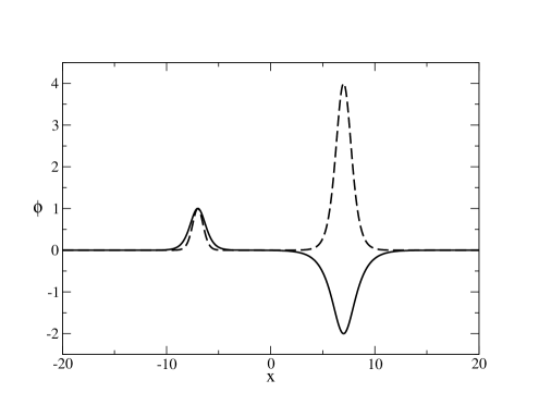
Figure 1: Illustration of solution (14) of Equation (13). Solid line: corresponding solution of the linear wave equation. The parameters of the solution are $F=1/\cosh^{2}(x+ct)$; $G=-2/\cosh(x-ct)$; $c=2.0$; $t=3.5$. Dashed line: solution (14). $\alpha=1/2$.

Figures 2 and 3 illustrate two interesting phenomena connected to some of the obtained solutions to the nonlinear differential equation. Figure 2 illustrates the occurrence of a wave and an antiwave from $\phi=0$ at $t=0$. This phenomenon is similar to the arising of a particle and antiparticle from the vacuum. Note that despite the fact that $\phi=0$ at $t=0$, the corresponding solution of (14) has an internal structure.

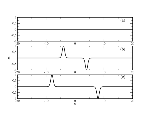
Figure 2: Illustration of the wave–antiwave phenomenon connected to solution (14) to the nonlinear partial differential Equation (13). The parameters of the solution are $F=1/\cosh^{2}(x+ct)$; $G=-1/\cosh^{2}(x-ct)$; $c=2.0$; $\alpha=1/3$. (a) $t=0$. (b) $t=2$. (c) $t=4$.

Figure 3 illustrates the phenomenon of a splitting of a nonlinear wave. This phenomenon is similar to the phenomenon of the splitting of a particle into two other particles. Note the nonlinearity of the superposition of the two waves in Figure 3.

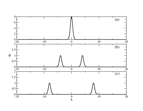
Figure 3: Illustration of the wave splitting phenomenon connected to solution (14) to the nonlinear partial differential Equation (13). The parameters of the solution are $F=1/\cosh^{2}(x+ct)$;$G=-1/\cosh^{2}(x-ct)$; $c=2.0$; $\alpha=1/3$. (a) $t=0$. (b) $t=2$. (c) $t=4$.

Proposition 3.

The equation

$$-\phi\frac{\partial^{2}\phi}{\partial t^{2}}+c^{2}\phi\frac{\partial^{2}\phi}{\partial x^{2}}+\left(\frac{\partial\phi}{\partial t}\right)^{2}-c^{2}\left(\frac{\partial\phi}{\partial x}\right)^{2}=0,$$ (20)

has the solutions

$$\phi(x,t)=\exp\Bigg{\{}F(x+ct)+G(x-ct)\Bigg{\}},$$ (21)

where $F$ and $G$ are arbitrary $C^{2}$-functions, and $-\infty\leq a<x<b\leq+\infty$, and $t>0$. Another solution is

$$\phi(x,t)=\exp\Bigg{\{}\frac{f(x+ct)+f(x-ct)}{2}+\frac{1}{2c}\int\limits_{x-ct}^{x+ct}ds\ g(s)\Bigg{\}},$$ (22)

for the conditions

$$\phi(x,0)=\exp[f(x)],\ \ \ \frac{\partial\ln(\phi)}{\partial t}(x,0)=g(x),\ \ -\infty<x<\infty,t>0,$$ (23)

and the solution

$$\phi(x,t)=\exp\Bigg{\{}\sum\limits_{n=1}^{\infty}\Bigg{[}a_{n}\cos\Bigg{(}\frac{n\pi ct}{L}\Bigg{)}+b_{n}\sin\Bigg{(}\frac{n\pi ct}{L}\Bigg{)}\Bigg{]}\sin\Bigg{(}\frac{n\pi x}{L}\Bigg{)}\Bigg{\}},$$

$$a_{n}=\frac{2}{L}\int\limits_{0}^{L}dx\ f(x)\sin\Bigg{(}\frac{n\pi x}{L}\Bigg{)},\ \ \ b_{n}=\frac{2}{n\pi c}\int\limits_{0}^{L}dx\ g(x)\sin\Bigg{(}\frac{n\pi x}{L}\Bigg{)},$$ (24)

for the case $0<x<L$ and initial and boundary conditions

$$\phi(x,0)=\exp[f(x)],\ \ \ \ \frac{\partial\ln(\phi)}{\partial t}(x,0)=g(x),\ \ 0\leq x\leq L$$

$$\frac{\partial\ln(\phi)}{\partial x}(0,t)=\frac{\partial ln(\phi)}{\partial x}(L,t)=0,\ \ t\geq 0.$$ (25)

Proof.

Let us consider the linear wave Equation (144). We performed the transformation

$$u=\ln(\phi).$$ (26)

The transformation (19) transforms Equation (144) to Equation (20). Equation (144) has the solutions (145), (147) and (A). Thus, Equation (13) has the solutions (21), (22) and (3). ∎

Figure 4 illustrates a solution of (20). Note that the transformation transforms the solution of the wave equation to a solution in which waves have non-negative values.

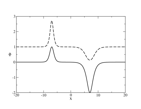
Figure 4: Illustration of solution (21) of Equation (20). Solid line: corresponding solution of the linear wave equation. The parameters of the solution are $F=1/\cosh^{2}(x+ct)$; $G=-2/\cosh(x-ct)$; $c=2.0$; $t=3.5$. Dashed line: solution (21).

Figure 5 illustrates the typical characteristics of soliton behavior for some of the obtained solutions. Figure 5a–c present a collision of two solitary waves which are described by a solution of Equation (20). We see that the form of the solitary waves after the collision is the same as their form before the collision. Figure 5b presents an interesting moment of the collision which is dominated by the wave of smaller amplitude. We note that for the classical solitons, the amplitude of the soliton is a function of its velocity. Figure 5 shows another kind of soliton. These solitons have different amplitudes but nevertheless travel with the same velocity. This property is quite interesting.

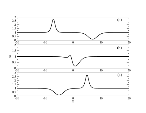
Figure 5: Illustration of the soliton properties of the waves connected to solution (21) of Equation (20). The parameters of the solution are $F=1/\cosh^{2}(x+ct)$; $G=-2/\cosh(x-ct)$; $c=2.0$. (a) $t=-2.5$. (b) $t=0.3$. (c) $t=3.5$.

The soliton properties of solution (21) to Equation (20) are also illustrated in Figure 6. We observe the collision of the two solitons. The solitons merge into a single solitary wave and then split again. The forms of the solitons do not change. Note, that the velocities of these solitons are the same despite the differences in their profiles.

Figure 6: Illustration of the soliton properties of the waves connected to solution (21) to Equation (20). The parameters of the solution are $F=0.7/\cosh^{2}(x+ct)$; $G=0.8/\cosh(x-ct)$; $c=2.0$.

Let us now consider a more complicated transformation: $u=u(\phi,\phi_{x})$.

Proposition 4.

The equation

$$c^{2}\phi\frac{\partial^{3}\phi}{\partial x^{3}}-\phi\frac{\partial^{3}\phi}{\partial x\partial t^{2}}+3c^{2}\frac{\partial\phi}{\partial x}\frac{\partial^{2}\phi}{\partial x^{2}}-\frac{\partial\phi}{\partial x}\frac{\partial\phi}{\partial t^{2}}-2\frac{\partial\phi}{\partial t}\frac{\partial^{2}\phi}{\partial x\partial t}=0,$$ (27)

has the solutions

$$\phi(x,t)=2^{1/2}\Bigg{\{}\int dx[F(x+ct)+G(x-ct)]\Bigg{\}}^{1/2},$$ (28)

where $F$ and $G$ are arbitrary $C^{2}$-functions, and $-\infty\leq a<x<b\leq+\infty$, and $t>0$. Another solution is

$$\phi(x,t)=2^{1/2}\Bigg{\{}\int dx\Bigg{[}\frac{f(x+ct)+f(x-ct)}{2}+\frac{1}{2c}\int\limits_{x-ct}^{x+ct}ds\ g(s)\Bigg{]}\Bigg{\}}^{1/2},$$ (29)

for the conditions

$$\phi(x,0)\frac{\partial\phi}{\partial x}(x,0)=f(x),\ \ \ \frac{\partial}{\partial t}\left[\phi\frac{\partial\phi}{\partial x}\right](x,0)=g(x),\ \ -\infty<x<\infty,t>0,$$ (30)

and the solution

$$\phi(x,t)=2^{1/2}\Bigg{\{}\int dx\Bigg{[}\sum\limits_{n=1}^{\infty}\Bigg{[}a_{n}\cos\Bigg{(}\frac{n\pi ct}{L}\Bigg{)}+b_{n}\sin\Bigg{(}\frac{n\pi ct}{L}\Bigg{)}\Bigg{]}\sin\Bigg{(}\frac{n\pi x}{L}\Bigg{)}\Bigg{]}\Bigg{\}}^{1/2},$$

$$a_{n}=\frac{2}{L}\int\limits_{0}^{L}dx\ f(x)\sin\Bigg{(}\frac{n\pi x}{L}\Bigg{)},\ \ \ b_{n}=\frac{2}{n\pi c}\int\limits_{0}^{L}dx\ g(x)\sin\Bigg{(}\frac{n\pi x}{L}\Bigg{)},$$ (31)

for the case $0<x<L$ and initial and boundary conditions

$$\phi(x,0)=2^{1/2}[\int dx\ f(x)]^{1/2},\ \ \ \ \frac{\partial}{\partial t}\left[\phi\frac{\partial\phi}{\partial x}\right](x,0)=g(x),\ \ 0\leq x\leq L$$

$$\frac{\partial}{\partial x}\left[\phi\frac{\partial\phi}{\partial x}\right](0,t)=\frac{\partial}{\partial x}\left[\phi\frac{\partial\phi}{\partial x}\right](L,t)=0,\ \ t\geq 0.$$ (32)

Proof.

Let us consider the linear wave Equation (144). We performed the transformation

$$u=\phi\frac{\partial\phi}{\partial x}.$$ (33)

The transformation (33) transforms Equation (144) to Equation (27). Equation (150) has the solutions (145), (147) and (A). Thus, Equation (27) has the solutions (28), (29) and (4). ∎

Note that (33) leads to $\phi=2^{1/2}\left(\int dx\ u\right)^{1/2}$.

Proposition 5.

The equation

$$(c^{2}-1)\frac{\partial^{3}\phi}{\partial x^{3}}+3c^{2}\frac{\partial\phi}{\partial x}\frac{\partial^{2}\phi}{\partial x^{2}}-3\frac{\partial\phi}{\partial t}\frac{\partial^{2}\phi}{\partial t^{2}}+c^{2}\left(\frac{\partial\phi}{\partial x}\right)^{3}-\left(\frac{\partial\phi}{\partial t}\right)^{3}=0,$$ (34)

has the solutions

$$\phi(x,t)=\ln\Bigg{\{}\int dx[F(x+ct)+G(x-ct)]\Bigg{\}},$$ (35)

where $F$ and $G$ are arbitrary $C^{2}$-functions, and $-\infty\leq a<x<b\leq+\infty$, and $t>0$. Another solution is

$$\phi(x,t)=\ln\Bigg{\{}\int dx\Bigg{[}\frac{f(x+ct)+f(x-ct)}{2}+\frac{1}{2c}\int\limits_{x-ct}^{x+ct}ds\ g(s)\Bigg{]}\Bigg{\}},$$ (36)

for the conditions

$$\exp[\phi(x,0)]\frac{\partial\phi}{\partial x}(x,0)=f(x),\ \ \ \frac{\partial}{\partial t}\left[\exp(\phi)\frac{\partial\phi}{\partial x}\right](x,0)=g(x),\ \ -\infty<x<\infty,t>0,$$ (37)

and the solution

$$\phi(x,t)=\ln\Bigg{\{}\int dx\Bigg{[}\sum\limits_{n=1}^{\infty}\Bigg{[}a_{n}\cos\Bigg{(}\frac{n\pi ct}{L}\Bigg{)}+b_{n}\sin\Bigg{(}\frac{n\pi ct}{L}\Bigg{)}\Bigg{]}\sin\Bigg{(}\frac{n\pi x}{L}\Bigg{)}\Bigg{]}\Bigg{\}},$$

$$a_{n}=\frac{2}{L}\int\limits_{0}^{L}dx\ f(x)\sin\Bigg{(}\frac{n\pi x}{L}\Bigg{)},\ \ \ b_{n}=\frac{2}{n\pi c}\int\limits_{0}^{L}dx\ g(x)\sin\Bigg{(}\frac{n\pi x}{L}\Bigg{)},$$ (38)

for the case $0<x<L$ and initial and boundary conditions

$$\phi(x,0)=\ln[\int dx\ f(x)],\ \ \ \ \frac{\partial}{\partial t}\left[\phi\frac{\partial\phi}{\partial x}\right](x,0)=g(x),\ \ 0\leq x\leq L$$

$$\frac{\partial}{\partial x}\left[\phi\frac{\partial\phi}{\partial x}\right](0,t)=\frac{\partial}{\partial x}\left[\phi\frac{\partial\phi}{\partial x}\right](L,t)=0,\ \ t\geq 0.$$ (39)

Proof.

Let us consider the linear wave Equation (144). We performed the transformation

$$u=\exp(\phi)\ \frac{\partial\phi}{\partial x}.$$ (40)

The transformation (40) transforms Equation (144) to Equation (34). Equation (150) has the solutions (145), (147) and (A). Thus, Equation (34) has the solutions (35), (36) and (5). ∎

Note that (40) leads to $\phi=\ln\left(\int dx\ u\right)$.

Proposition 6.

The equation

$$2\phi\left[c^{2}\left(\frac{\partial^{2}\phi}{\partial x^{2}}\right)^{2}-\left(\frac{\partial^{2}\phi}{\partial x\partial t}\right)^{2}\right]+\left(\frac{\partial\phi}{\partial x}\right)^{2}\left[c^{2}\frac{\partial^{2}\phi}{\partial x^{2}}-\frac{\partial^{2}\phi}{\partial t^{2}}\right]-$$

$$2\frac{\partial\phi}{\partial x}\left(c^{2}\frac{\partial\phi}{\partial x}\frac{\partial^{2}\phi}{\partial x^{2}}-\frac{\partial\phi}{\partial t}\frac{\partial^{2}\phi}{\partial x\partial t}\right)-\phi\frac{\partial\phi}{\partial x}\left(c^{2}\frac{\partial^{3}\phi}{\partial x^{3}}-\frac{\partial\phi}{\partial x\partial t^{2}}\right)=0,$$ (41)

has the solutions

$$\phi(x,t)=\exp\Bigg{\{}\int dx\frac{1}{[F(x+ct)+G(x-ct)]}\Bigg{\}},$$ (42)

where $F$ and $G$ are arbitrary $C^{2}$-functions, and $-\infty\leq a<x<b\leq+\infty$, and $t>0$. Another solution is

$$\phi(x,t)=\exp\Bigg{\{}\int dx\frac{1}{\Bigg{[}\frac{f(x+ct)+f(x-ct)}{2}+\frac{1}{2c}\int\limits_{x-ct}^{x+ct}ds\ g(s)\Bigg{]}}\Bigg{\}},$$ (43)

for the conditions

$$\phi(x,0)]\frac{\partial\phi}{\partial x}(x,0)=f(x),\ \ \ \frac{\partial}{\partial t}\left[\phi\frac{\partial\phi}{\partial x}\right](x,0)=g(x),\ \ -\infty<x<\infty,t>0,$$ (44)

and the solution

$$\phi(x,t)=\exp\Bigg{\{}\int dx\frac{1}{\Bigg{[}\sum\limits_{n=1}^{\infty}\Bigg{[}a_{n}\cos\Bigg{(}\frac{n\pi ct}{L}\Bigg{)}+b_{n}\sin\Bigg{(}\frac{n\pi ct}{L}\Bigg{)}\Bigg{]}\sin\Bigg{(}\frac{n\pi x}{L}\Bigg{)}\Bigg{]}}\Bigg{\}},$$

$$a_{n}=\frac{2}{L}\int\limits_{0}^{L}dx\ f(x)\sin\Bigg{(}\frac{n\pi x}{L}\Bigg{)},\ \ \ b_{n}=\frac{2}{n\pi c}\int\limits_{0}^{L}dx\ g(x)\sin\Bigg{(}\frac{n\pi x}{L}\Bigg{)},$$ (45)

for the case $0<x<L$ and initial and boundary conditions

$$\phi(x,0)=\exp\left[\int dx\frac{1}{f(x)}\right],\ \ \ \ \frac{\partial}{\partial t}\left[\phi\Bigg{/}\frac{\partial\phi}{\partial x}\right](x,0)=g(x),\ \ 0\leq x\leq L$$

$$\frac{\partial}{\partial x}\left[\phi\Bigg{/}\frac{\partial\phi}{\partial x}\right](0,t)=\frac{\partial}{\partial x}\left[\phi\Bigg{/}\frac{\partial\phi}{\partial x}\right](L,t)=0,\ \ t\geq 0.$$ (46)

Proof.

Let us consider the linear wave Equation (144). We performed the transformation

$$u=\phi\Bigg{/}\frac{\partial\phi}{\partial x}.$$ (47)

The transformation (47) transforms Equation (144) to Equation (6). Equation (150) has the solutions (145), (147) and (A). Thus, Equation (6) has the solutions (42), (43) and (6). ∎

Note that (47) leads to $\phi=\exp\left(\int dx\ (1/u)\right)$.

2.2 Transformations for the Heat Equation

The solutions of the linear heat Equation (150) are presented in the Appendix A.

Proposition 7.

The equation

$$\frac{\partial\phi}{\partial t}-a^{2}\left(\frac{\partial\phi}{\partial x}\right)^{2}-a^{2}\frac{\partial^{2}\phi}{\partial x^{2}}=0,$$ (48)

has the solutions

$$\phi(x,t)=\ln\Bigg{(}\frac{1}{2a\sqrt{\pi t}}\Bigg{)}+\ln\Bigg{\{}\int\limits_{-\infty}^{+\infty}d\xi\ f(\xi)\exp\left[-\frac{(\xi-x)^{2}}{4at^{2}}\right]\Bigg{\}},$$ (49)

for the case $-\infty<x<\infty$ and for the initial condition $\phi(x,0)=\ln[f(x)]$, and the solution

$$\phi(x,t)=\ln\Bigg{\{}A+\frac{B-A}{L}+\sum\limits_{n=1}^{\infty}a_{n}\exp\Bigg{(}-\frac{\pi^{2}a^{2}n^{2}}{L^{2}}t\Bigg{)}\sin\Bigg{(}\frac{n\pi x}{L}\Bigg{)}$$

$$a_{n}=-\frac{2}{n\pi}[A+(-1)^{n+1}B]+\frac{2}{L}\int\limits_{0}^{L}dx\ f(x)\sin\Bigg{(}\frac{n\pi x}{L}\Bigg{)}\Bigg{\}},$$ (50)

for the case $0<x<L$ and initial and boundary conditions $\phi(x,0)=\ln[f(x)]$ and $\phi(0,t)=\ln(A)$, $\phi(L,t)=ln(B)$.

Proof.

Let us consider the linear heat Equation (150). We use the transformation

$$u=\exp(\phi).$$ (51)

The transformation (12) transforms Equation (150) to Equation (48). Equation (150) has the solutions (151) and (A). Thus, Equation (48) has the solutions (49) and (7). ∎

We can make the transformation more complicated. This more complicated transformation will transform the linear heat equation into a nonlinear Burgers equation. The transformation is the inverse transformation of the Hopf–Cole transformation.

Proposition 8.

The equation

$$\frac{\partial\phi}{\partial t}+\phi\frac{\partial\phi}{\partial x}+a^{2}\frac{\partial^{2}\phi}{\partial x^{2}}=0,$$ (52)

has the solutions

$$\phi(x,t)=-2a^{2}\frac{\frac{\partial}{\partial x}\int\limits_{-\infty}^{+\infty}d\xi\ f(\xi)\exp\left[-\frac{(\xi-x)^{2}}{4at^{2}}\right]}{\int\limits_{-\infty}^{+\infty}d\xi\ f(\xi)\exp\left[-\frac{(\xi-x)^{2}}{4at^{2}}\right]},$$ (53)

for the case $-\infty<x<\infty$ and for the initial condition $\phi(x,0)=-2\frac{a^{2}}{f}\frac{df}{dx}$, and the solution

$$\phi(x,t)=-2a^{2}\frac{\sum\limits_{n=1}^{\infty}\frac{n\pi a_{n}}{L}\exp\Bigg{(}-\frac{\pi^{2}a^{2}n^{2}}{L^{2}}t\Bigg{)}\sin\Bigg{(}\frac{n\pi x}{L}\Bigg{)}}{A+\frac{B-A}{L}+\sum\limits_{n=1}^{\infty}a_{n}\exp\Bigg{(}-\frac{\pi^{2}a^{2}n^{2}}{L^{2}}t\Bigg{)}\sin\Bigg{(}\frac{n\pi x}{L}\Bigg{)}},$$ (54)

for the case $0<x<L$ and initial and boundary conditions $\phi(x,0)=-2\frac{a^{2}}{f}\frac{df}{dx}$ and $\phi(0,t)=0$, $\phi(L,t)=0$.

Proof.

Let us consider Equation (150). We apply the transformation

$$u=\exp\left(-\frac{1}{2a^{2}}\int dx\ \phi(x,t)\right).$$ (55)

The transformation transforms (150) to Equation (52). Thus, Equation (52) has solutions (53) and (54). ∎

We note that the transformation (55) leads to

$$\phi=-2a^{2}\frac{1}{u}\frac{\partial u}{\partial x},$$ (56)

which is the Hopf–Cole transformation.

Proposition 9.

The equation

$$\phi\frac{\partial\phi}{\partial t}+\phi^{3}\frac{\partial\phi}{\partial x}+a^{2}\left(\frac{\partial\phi}{\partial x}\right)^{2}+a^{2}\phi\frac{\partial^{2}\phi}{\partial x^{2}}=0,$$ (57)

has the solutions

$$\phi(x,t)=\phi(x,t)=\left\{2a^{2}\frac{\frac{\partial}{\partial x}\int\limits_{-\infty}^{+\infty}d\xi\ f(\xi)\exp\left[-\frac{(\xi-x)^{2}}{4at^{2}}\right]}{\int\limits_{-\infty}^{+\infty}d\xi\ f(\xi)\exp\left[-\frac{(\xi-x)^{2}}{4at^{2}}\right]}\right\}^{1/2},$$ (58)

for the case $-\infty<x<\infty$ and for the initial condition $\phi(x,0)=\left[2a^{2}\frac{1}{f(x)}\frac{df}{dx}\right]^{1/2}$, and the solution

$$\phi(x,t)=\phi(x,t)=\left\{2a^{2}\frac{\sum\limits_{n=1}^{\infty}\frac{n\pi a_{n}}{L}\exp\Bigg{(}-\frac{\pi^{2}a^{2}n^{2}}{L^{2}}t\Bigg{)}\sin\Bigg{(}\frac{n\pi x}{L}\Bigg{)}}{A+\frac{B-A}{L}+\sum\limits_{n=1}^{\infty}a_{n}\exp\Bigg{(}-\frac{\pi^{2}a^{2}n^{2}}{L^{2}}t\Bigg{)}\sin\Bigg{(}\frac{n\pi x}{L}\Bigg{)}}\right\}^{1/2},$$ (59)

for the case $0<x<L$ and initial and boundary conditions $\phi(x,0)=\left[2a^{2}\frac{1}{f(x)}\frac{df}{dx}\right]^{1/2}$ and $\phi(0,t)=0$, $\phi(L,t)=0$.

Proof.

Let us consider Equation (150). Equation (57) has the solution

$$\phi=\left(2a^{2}\frac{1}{u}\frac{\partial u}{\partial x}\right)^{1/2},$$ (60)

and, thus, we arrive at the solutions (58) and (59). ∎

Proposition 10.

The equation

$$(\alpha-1)a^{2}\left(\frac{\partial\phi}{\partial x}\right)^{2}-a\phi\frac{\partial^{2}\phi}{\partial x^{2}}-\phi\frac{\partial\phi}{\partial t}=0,$$ (61)

has the solutions

$$\phi(x,t)=\Bigg{\{}\frac{1}{2a\sqrt{\pi t}}\int\limits_{-\infty}^{+\infty}d\xi\ f(\xi)\exp\left[-\frac{(\xi-x)^{2}}{4at^{2}}\right]\Bigg{\}}^{1/\alpha},$$ (62)

for the case $-\infty<x<\infty$ and for the initial condition $\phi(x,0)=[f(x)]^{1/\alpha}$, and the solution

$$\phi(x,t)=\Bigg{\{}A+\frac{B-A}{L}+\sum\limits_{n=1}^{\infty}a_{n}\exp\Bigg{(}-\frac{\pi^{2}a^{2}n^{2}}{L^{2}}t\Bigg{)}\sin\Bigg{(}\frac{n\pi x}{L}\Bigg{)}$$

$$a_{n}=-\frac{2}{n\pi}[A+(-1)^{n+1}B]+\frac{2}{L}\int\limits_{0}^{L}dx\ f(x)\sin\Bigg{(}\frac{n\pi x}{L}\Bigg{)}\Bigg{\}}^{1/\alpha},$$ (63)

for the case $0<x<L$ and initial and boundary conditions $\phi(x,0)=[f(x)]^{1/\alpha}$ and $\phi(0,t)=A^{1/\alpha}$, $\phi(L,t)=B^{1/\alpha}$.

Proof.

Let us consider the linear heat Equation (150). We use the transformation

$$u=\phi^{\alpha},\alpha\neq 1.$$ (64)

The transformation (64) transforms Equation (150) to Equation (61). Equation (150) has the solutions (151) and (A). Thus, Equation (61) has the solutions (62) and (10). ∎

Proposition 11.

The equation

$$a^{2}\frac{\partial^{3}\phi}{\partial x^{3}}+2a\phi\frac{\partial\phi}{\partial x}\frac{\partial^{2}\phi}{\partial x^{2}}+\alpha^{2}\frac{\partial\phi}{\partial x}\left(\frac{\partial\phi}{\partial x}\right)^{2}+a^{2}\frac{\partial\phi}{\partial x}-\phi\left(\frac{\partial\phi}{\partial t}\right)^{2}-\phi\frac{\partial^{2}\phi}{\partial t}=0,$$ (65)

has the solutions

$$\phi(x,t)=2^{1/2}\Bigg{\{}\int dx\ \Bigg{\{}\frac{1}{2a\sqrt{\pi t}}\int\limits_{-\infty}^{+\infty}d\xi\ f(\xi)\exp\left[-\frac{(\xi-x)^{2}}{4at^{2}}\right]\Bigg{\}}\Bigg{\}}^{1/2},$$ (66)

for the case $-\infty<x<\infty$ and for the initial condition $\phi(x,0)=2^{1/2}[\int dx\ f(x)]^{1/2}$, and the solution

$$\phi(x,t)=2^{1/2}\Bigg{\{}\int dx\Bigg{\{}A+\frac{B-A}{L}+\sum\limits_{n=1}^{\infty}a_{n}\exp\Bigg{(}-\frac{\pi^{2}a^{2}n^{2}}{L^{2}}t\Bigg{)}\sin\Bigg{(}\frac{n\pi x}{L}\Bigg{)}\Bigg{\}}\Bigg{\}}^{1/2}$$

$$a_{n}=-\frac{2}{n\pi}[A+(-1)^{n+1}B]+\frac{2}{L}\int\limits_{0}^{L}dx\ f(x)\sin\Bigg{(}\frac{n\pi x}{L}\Bigg{)},$$ (67)

for the case $0<x<L$ and initial and boundary conditions $\phi(x,0)=2^{1/2}[\int dx\ f(x)]^{1/2}$ and $\phi(0,t)=2^{1/2}[\int dxA]^{1/2}$, $\phi(L,t)=2^{1/2}(\int dxB)^{1/2}$.

Proof.

Let us consider the linear heat Equation (150). We use the transformation

$$u=\phi\frac{\partial\phi}{\partial x}.$$ (68)

The transformation (68) transforms Equation (150) to Equation (65). Equation (150) has the solutions (151) and (A). Thus, Equation (65) has the solutions (66) and (11). ∎

Proposition 12.

The equation

$$a^{2}\left(\frac{\partial\phi}{\partial x}\right)^{3}+2a^{2}\phi\frac{\partial^{2}\phi}{\partial x^{2}}+a^{2}\frac{\partial\phi}{\partial x}\frac{\partial^{2}\phi}{\partial x^{2}}+a^{2}\frac{\partial^{3}\phi}{\partial x^{3}}-\frac{\partial\phi}{\partial x}\frac{\partial\phi}{\partial t}-\frac{\partial^{2}\phi}{\partial x\partial t}=0,$$ (69)

has the solutions

$$\phi(x,t)=\ln\Bigg{\{}\int dx\ \Bigg{\{}\frac{1}{2a\sqrt{\pi t}}\int\limits_{-\infty}^{+\infty}d\xi\ f(\xi)\exp\left[-\frac{(\xi-x)^{2}}{4at^{2}}\right]\Bigg{\}}\Bigg{\}},$$ (70)

for the case $-\infty<x<\infty$ and for the initial condition $\phi(x,0)=[\int dx\ f(x)]$, and the solution

$$\phi(x,t)=\int dx\Bigg{\{}A+\frac{B-A}{L}+\sum\limits_{n=1}^{\infty}a_{n}\exp\Bigg{(}-\frac{\pi^{2}a^{2}n^{2}}{L^{2}}t\Bigg{)}\sin\Bigg{(}\frac{n\pi x}{L}\Bigg{)}\Bigg{\}}$$

$$a_{n}=-\frac{2}{n\pi}[A+(-1)^{n+1}B]+\frac{2}{L}\int\limits_{0}^{L}dx\ f(x)\sin\Bigg{(}\frac{n\pi x}{L}\Bigg{)},$$ (71)

for the case $0<x<L$ and initial and boundary conditions $\phi(x,0)=\int dx\ f(x)]$ and$\phi(0,t)=2^{1/2}[\int dxA]^{1/2}$, $\phi(L,t)=2^{1/2}(\int dxB)^{1/2}$.

Proof.

Let us consider the linear heat Equation (150). We use the transformation

$$u=\exp(\phi)\frac{\partial\phi}{\partial x}.$$ (72)

The transformation (72) transforms Equation (150) to Equation (69). Equation (150) has the solutions (151) and (A). Thus, Equation (69) has the solutions (70) and (12). ∎

2.3 Transformation for the Laplace Equation

The used solution of the Laplace Equation (153) is given in Appendix A.

Proposition 13.

The equation

$$\left(\frac{\partial\phi}{\partial x}\right)^{2}+\left(\frac{\partial\phi}{\partial y}\right)^{2}+\frac{\partial^{2}\phi}{\partial x^{2}}+\frac{\partial^{2}\phi}{\partial y^{2}}=0,$$ (73)

for the case of the rectangle domain $a<x<b$, $c<x<d$ and boundary conditions $\phi(a,y)=\ln[f(y)]$; $\phi(b,y)=\ln[g(y)]$; $\phi(x,c)=\ln[h(c)]$; $\phi(x,d)=\ln[k(x)]$, has the solution

$$\phi=\ln(u_{1}+u_{2});\ \ \ u_{1}=\sum\limits_{n}X_{n}(x)Y_{n}(y);\ \ \ u_{2}=\sum\limits_{m}Z_{m}(x)V_{m}(y).$$ (74)

Proof.

Let us consider the linear Laplace equation (153) We make the transformation

$$u=\exp(\phi).$$ (75)

The transformation (75) transforms Equation (153) to Equation (73). Equation (153) has the solution (154) Thus, Equation (73) has the solutions (74). ∎

Proposition 14.

The equation

$$\phi\frac{\partial^{3}\phi}{\partial x^{3}}+3\frac{\partial\phi}{\partial x}\frac{\partial^{2}\phi}{\partial x^{2}}+\frac{\partial\phi}{\partial x}\frac{\partial^{2}\phi}{\partial y^{2}}+2\frac{\partial\phi}{\partial y}\frac{\partial^{2}\phi}{\partial x\partial y}+\phi\frac{\partial^{3}\phi}{\partial x\partial y^{2}}=0,$$ (76)

for the case of the rectangle domain $a<x<b$, $c<x<d$ and boundary conditions$\phi(a,y)=2^{1/2}\{\int dx[f(y)]\}^{1/2}$; $\phi(b,y)=2^{1/2}\{\int dx[g(y)]\}^{1/2}$; $\phi(x,c)=2^{1/2}\{\int dx[h(c)]\}^{1/2}$; $\phi(x,d)=2^{1/2}\{\int dx[k(x)]\}^{1/2}$, has the solution

$$\phi=2^{1/2}\left\{\int dx(u_{1}+u_{2})\right\}^{1/2};\ \ \ u_{1}=\sum\limits_{n}X_{n}(x)Y_{n}(y);\ \ \ u_{2}=\sum\limits_{m}Z_{m}(x)V_{m}(y).$$ (77)

Proof.

Let us consider the linear Laplace Equation (153). We use the transformation

$$u=\phi\frac{\partial\phi}{\partial x}.$$ (78)

The transformation (78) transforms Equation (153) to Equation (76). Equation (153) has the solution (154) Thus, Equation (76) has the solution (77). ∎

Proposition 15.

The equation

$$(\alpha-1)\left[\left(\frac{\partial\phi}{\partial x}\right)^{2}+\left(\frac{\partial\phi}{\partial y}\right)^{2}\right]+\phi\left(\frac{\partial^{2}\phi}{\partial x^{2}}+\frac{\partial^{2}\phi}{\partial y^{2}}\right)=0,$$ (79)

for the case of the rectangle domain $a<x<b$, $c<x<d$ and boundary conditions $\phi(a,y)=[f(y)]^{1/\alpha}$; $\phi(b,y)=[g(y)]^{1/\alpha}$; $\phi(x,c)=[h(c)]^{1/\alpha}$; $\phi(x,d)=[k(x)]^{1/\alpha}$, has the solution The solution is

$$\phi=(u_{1}+u_{2})^{1/\alpha};\ \ \ u_{1}=\sum\limits_{n}X_{n}(x)Y_{n}(y);\ \ \ u_{2}=\sum\limits_{m}Z_{m}(x)V_{m}(y).$$ (80)

Proof.

Let us consider the linear Laplace Equation (153). We make the transformation

$$u=\phi^{\alpha},\alpha\neq 1,$$ (81)

where $\alpha$ =const. The transformation (81) transforms Equation (153) to Equation (79). Equation (153) has the solution (154) Thus, Equation (79) has the solution (80). ∎

3 Transformations of Linear and Nonlinear Ordinary Differential Equations

The main idea above was to start from linear partial differential equations and by means of appropriate transformations to obtain solutions of nonlinear differential equations.

We can start from linear ordinary differential equations and obtain solutions of nonlinear ordinary differential equations. Let us consider, for example, the linear ordinary differential equation

$$\frac{du}{dx}+p(x)u=q(x).$$ (82)

The solution of this equation is

$$u(x)=\exp\left(-\int dx\ p(x)\right)\left[C+\int dx\ q(x)\exp\left(\int dx\ p(x)\right)\right].$$ (83)

$C$ in (83) is a constant of integration. The Cauchy problem $u(x_{0})=u_{0}$ for (82) has the solution

$$u(x)=\exp\left(-\int\limits_{x_{0}}^{x}dy\ p(y)\right)\left[u_{0}+\int\limits_{x_{0}}^{x}dy\ q(x)\exp\left(\int\limits_{x_{0}}^{x}dy\ p(y)\right)\right].$$ (84)

Proposition 16.

The nonlinear differential equation

$$\phi\frac{d^{2}\phi}{dx^{2}}+\left(\frac{\partial\phi}{\partial x}\right)^{2}+p(x)\phi\frac{d\phi}{dx}=q(x),$$ (85)

has the solution

$$\phi=2^{1/2}\left\{\int dx\left\{\exp\left(-\int dx\ p(x)\right)\left[C+\int dx\ q(x)\exp\left(\int dx\ p(x)\right)\right]\right\}\right\}^{1/2}.$$ (86)

The Cauchy problem $u(x_{0})=u_{0}$ for (85) has the solution

$$u(x)=2^{1/2}\left\{\exp\left(-\int\limits_{x_{0}}^{x}dy\ p(y)\right)\left[u_{0}+\int\limits_{x_{0}}^{x}dy\ q(x)\exp\left(\int\limits_{x_{0}}^{x}dy\ p(y)\right)\right]\right\}^{1/2}.$$ (87)

Proof.

Let us apply the transformation

$$u=\phi(x)\frac{d\phi}{dx}.$$ (88)

(88) transforms (82) to (85) and the solutions (83) and (84) are transformed to (86) and (87). ∎

Proposition 17.

Let us consider the equation

$$\frac{d^{2}\phi}{dx^{2}}+\left(\frac{d\phi}{dx}\right)^{2}+p(x)\frac{d\phi}{dx}-q(x)\exp(-\phi)=0.$$ (89)

The solution of (89) is

$$\phi(x)=\ln\left\{\int dx\left\{\exp\left(-\int dx\ p(x)\right)\left[C+\int dx\ q(x)\exp\left(\int dx\ p(x)\right)\right]\right\}\right\}.$$ (90)

The Cauchy problem $u(x_{0})=u_{0}$ for (89) has the solution

$$u(x)=\ln\left\{\int dx\left\{\left(-\int\limits_{x_{0}}^{x}dy\ p(y)\right)\left[u_{0}+\int\limits_{x_{0}}^{x}dy\ q(x)\exp\left(\int\limits_{x_{0}}^{x}dy\ p(y)\right)\right]\right\}\right\}.$$ (91)

Proof.

Let us now apply the transformation

$$u=\exp(\phi)\frac{d\phi}{dx}.$$ (92)

The transformation (92) transforms (82) to (89). The solutions (83) and (84) are transformed to (90) and (91). ∎

Our last example here will be connected to the equation

$$\frac{d^{2}u}{dx^{2}}+a\frac{du}{dx}+bu=0.$$ (93)

The solution of (93) depends on the characteristic numbers $\lambda_{1,2}=-\frac{a}{2}\mp\sqrt{\frac{a^{2}}{4}-b}$. The solution is

$$u=C_{1}\exp(\lambda_{1}x)+C_{2}\exp(\lambda_{2}x),\ \ \lambda_{1}\neq\lambda_{2},$$ (94)

and

$$u=(C_{1}+C_{2}x)\exp(\lambda x),\ \ \lambda_{1}=\lambda_{2}=\lambda.$$ (95)

$C_{1,2}$ are constants. Let us apply the transformation $u=\phi^{\alpha}$. (93) is transformed to

$$\alpha(\alpha-1)\left(\frac{d\phi}{dx}\right)^{2}+\alpha\phi\frac{d^{2}\phi}{dx^{2}}+\alpha a\phi\frac{d\phi}{dx}+b\phi=0.$$ (96)

The solutions of (96) are

$$\phi=[C_{1}\exp(\lambda_{1}x)+C_{2}\exp(\lambda_{2}x)]^{1/\alpha},\ \ \lambda_{1}\neq\lambda_{2},$$ (97)

and

$$\phi=[(C_{1}+C_{2}x)\exp(\lambda x)]^{1/\alpha},\ \ \lambda_{1}=\lambda_{2}=\lambda.$$ (98)

Proposition 18.

Let us consider the equation

$$\frac{d^{3}\phi}{dx^{3}}+3\frac{d\phi}{dx}\frac{d^{2}\phi}{dx^{2}}+\left(\frac{d\phi}{dx}\right)^{3}+a\frac{d^{2}\phi}{dx^{2}}+a\left(\frac{d\phi}{dx}\right)^{2}+b\exp(\phi)\frac{d\phi}{dx}=0.$$ (99)

(99) has the solutions

$$\phi=\ln\{\int dx[C_{1}\exp(\lambda_{1}x)+C_{2}\exp(\lambda_{2}x)]\},\ \ \lambda_{1}\neq\lambda_{2},$$ (100)

and

$$\phi=\ln\{\int dx[(C_{1}+C_{2}x)\exp(\lambda x)]\},\ \ \lambda_{1}=\lambda_{2}.$$ (101)

Proof.

We apply the transformation $u=\exp(\phi)\frac{d\phi}{dx}$ to (93). (93) is transformed to Equation (96) and solutions (97) and (98) are transformed to (100) and (101). ∎

Proposition 19.

The equation

$$\frac{d^{2}\phi}{dx^{2}}+\left(\frac{d\phi}{dx}\right)^{2}+a\frac{d\phi}{dx}+b\exp(\phi)=0,$$ (102)

has the solutions

$$\phi=\ln[C_{1}\exp(\lambda_{1}x)+C_{2}\exp(\lambda_{2}x)],\ \ \lambda_{1}\neq\lambda_{2},$$ (103)

and

$$\phi=\ln[(C_{1}+C_{2}x)\exp(\lambda x)],\ \ \lambda_{1}=\lambda_{2}=\lambda.$$ (104)

Proof.

We make the transformation $u=\exp(\phi)$. Equation (93) is transformed to (102). Solutions (97) and (98) are transformed to solutions (103) and (104). ∎

We can start from nonlinear ordinary differential equations and we can obtain solutions of other nonlinear differential equations. Let us consider as examples the equations of Bernoulli and Riccati. The equation of Bernoulli

$$\frac{d\phi}{dx}+p(x)\phi=q(x)\phi^{m},\ m\neq 0,\ m\neq 1,$$ (105)

is an example of a nonlinear equation which can be obtained from a linear equation by means of a transformation. The linear equation is

$$\frac{du}{dx}+(1-m)p(x)u=(1-m)q(x),$$ (106)

and the transformation is $u=\phi^{1-m}$. The solution of the linear equation is

$$u(x)=\exp\left[-(1-m)\int dxp(x)\right]\left\{C+(1-m)\int dx\ q(x)\exp\left[(1-m)\int dx\ p(x)\right]\right\}.$$ (107)

Thus, the solution of the Bernoulli equation is

$$\phi=\left\{\exp\left[-(1-m)\int dx\ p(x)\right]\left\{C+(1-m)\int dx\ q(x)\exp\left[(1-m)\int dx\ p(x)\right]\right\}\right\}^{1/(1-m)}.$$ (108)

Proposition 20.

The equation

$$\frac{d\psi}{dx}+p(x)-q(x)\exp[(m-1)\psi]=0,$$ (109)

has the solution

$$\psi=\ln\Bigg{\{}\Bigg{\{}\exp\left[-(1-m)\int dx\ p(x)\right]\Bigg{\{}C+(1-m)\times$$

$$\int dx\ q(x)\exp\left[(1-m)\int dx\ p(x)\right]\Bigg{\}}\Bigg{\}}^{1/(1-m)}\Bigg{\}}.$$ (110)

Proof.

Let us apply the transformation $\phi=\exp(\psi)$. This transformation transforms the equation of Bernoulli (105) to Equation (109) and solution (108) is transformed to (20). ∎

Proposition 21.

The equation

$$\left(\frac{d\psi}{dx}\right)^{2}+\frac{d^{2}\psi}{dx^{2}}+p(x)\frac{d\psi}{dx}-q(x)\exp[(m-1)\psi]\left(\frac{d\psi}{dx}\right)^{m}=0,$$ (111)

has the solution

$$\psi=\ln\Bigg{\{}\int dx\Bigg{\{}\Bigg{\{}\exp\left[-(1-m)\int dx\ p(x)\right]\Bigg{\{}C+(1-m)\times$$

$$\int dx\ q(x)\exp\left[(1-m)\int dx\ p(x)\right]\Bigg{\}}\Bigg{\}}^{1/(1-m)}\Bigg{\}}\Bigg{\}}.$$ (112)

Proof.

Let us apply the transformation $\phi=\exp(\psi)\frac{d\psi}{dx}$. This transformation transforms the equation of Bernoulli (105) to Equation (111) and solution (108) is transformed to (21). ∎

Next, we discuss the equation of Riccati. We shall consider the specific case of the Riccati equation, which has the constant coefficients

$$\frac{du}{dx}=\alpha_{2}u^{2}+\alpha_{1}u+\alpha_{0}.$$ (113)

The general solution of this equation is

$$u(t)=-\frac{\alpha_{1}}{2\alpha_{2}}-\frac{\theta}{2\alpha_{2}}\tanh\left[\frac{\theta(x+C)}{2}\right]+\frac{D}{\cosh^{2}\left[\frac{\theta(x+C)}{2}\right]\left\{E-\frac{2\alpha_{2}D}{\theta}\tanh\left[\frac{\theta(x+C)}{2}\right]\right\}},$$ (114)

where $\theta^{2}=\alpha_{1}^{2}-4\alpha_{0}\alpha_{2}$, and $C,D,E$ are constants.

Proposition 22.

The equation

$$\frac{d\phi}{dx}=a_{2}\exp(\phi)+a_{1}+a_{0}\exp(-\phi),$$ (115)

has the solution

$$\phi=\ln\Bigg{\{}-\frac{\alpha_{1}}{2\alpha_{2}}-\frac{\theta}{2\alpha_{2}}\tanh\left[\frac{\theta(x+C)}{2}\right]+\frac{D}{\cosh^{2}\left[\frac{\theta(x+C)}{2}\right]\left\{E-\frac{2\alpha_{2}D}{\theta}\tanh\left[\frac{\theta(x+C)}{2}\right]\right\}}\Bigg{\}}.$$ (116)

Note the following specific cases of (115). Let $a_{2}=a_{0}=a/2$. Then, we obtain the equation

$$\frac{\partial\psi}{\partial x}=a_{1}+a\cosh(\psi).$$ (117)

Let $a_{2}-a_{0}=a/2$. Then, we obtain the equation

$$\frac{\partial\psi}{\partial x}=a_{1}+a\sinh(\psi).$$ (118)

Proof.

Let us apply the transformation $\phi=\exp(\psi)$. This transformation transforms the equation of Riccati (113) to Equation (115) and solution (114) is transformed to (116). ∎

Proposition 23.

The equation

$$\frac{d^{2}\psi}{dx^{2}}+\left(\frac{d\psi}{dx}\right)^{2}=a_{2}\exp(\psi)\left(\frac{d\psi}{dx}\right)^{2}+a_{1}\frac{d\psi}{dx}+a_{0}\exp(-\psi),$$ (119)

has the solution

$$\phi=\ln\Bigg{\{}\int dx\Bigg{\{}-\frac{\alpha_{1}}{2\alpha_{2}}-\frac{\theta}{2\alpha_{2}}\tanh\left[\frac{\theta(x+C)}{2}\right]+\frac{D}{\cosh^{2}\left[\frac{\theta(x+C)}{2}\right]\left\{E-\frac{2\alpha_{2}D}{\theta}\tanh\left[\frac{\theta(x+C)}{2}\right]\right\}}\Bigg{\}}\Bigg{\}}.$$ (120)

Proof.

Let us apply the transformation $\phi=\exp(\psi)\frac{d\psi}{dx}$. This transformation transforms the equation of Riccati (113) to Equation (119) and solution (114) is transformed to (120). ∎

Proposition 24.

The equation

$$\alpha\frac{d\phi}{dx}=a_{2}\phi^{\alpha+1}+a_{1}\psi+a_{0}\phi^{1-\alpha},$$ (121)

has the solution

$$\phi=\Bigg{\{}-\frac{\alpha_{1}}{2\alpha_{2}}-\frac{\theta}{2\alpha_{2}}\tanh\left[\frac{\theta(x+C)}{2}\right]+\frac{D}{\cosh^{2}\left[\frac{\theta(x+C)}{2}\right]\left\{E-\frac{2\alpha_{2}D}{\theta}\tanh\left[\frac{\theta(x+C)}{2}\right]\right\}}\Bigg{\}}^{1/\alpha}.$$ (122)

Proof.

Let us apply the transformation $\phi=\psi^{\alpha}$ ($\alpha\neq 1$). This transformation transforms the equation of Riccati (113) to Equation (121) and solution (114) is transformed to (122). ∎

4 Transformations of Nonlinear Partial Differential Equations

We can also start from nonlinear partial differential equations and we can obtain solutions of other nonlinear partial differential equations by applying appropriate transformations. Here, we consider as an example the Korteweg–de Vries equation

$$\frac{\partial u}{\partial t}+\frac{\partial^{3}u}{\partial x^{3}}-6u\frac{\partial u}{\partial x}=0.$$ (123)

The single soliton solution of (123) is given by

$$u(x,t)=-\frac{c}{2}{\rm sech}^{2}\left[\frac{\sqrt{c}}{2}(x-ct)\right],$$ (124)

where $c$ is the velocity of the wave. The N-soliton solution of (123) is given by

$$u(x,t)=-2\frac{\partial^{2}}{\partial x^{2}}\ln\det[A(x,t)],$$ (125)

where the matrix $A_{nm}$ is

$$A_{nm}(x,t)=\delta_{nm}+\frac{\beta_{n}\exp(8\xi_{n}^{3}t)\exp[-(\xi_{n}+\xi_{m})x]}{\xi_{n}+\xi_{n}}.$$

Above, the parameters $\xi_{1}\geq xi_{2}\geq\dots,\geq\xi_{N}>0$ and the parameters $\beta_{i}$ , $i=1,\dots,N$ are nonzero ones.

The bisoliton solution of the Korteweg–de Vries equation which satisfies the initial condition $u(x,0)=$-$6{\rm sech}^{2}{(x)}$ is

$$u(x,t)=-12\frac{3+4\cosh(8t-2x)+\cosh(64t-4x)}{[\cosh(36t-3x)+3\cosh(28t-x)]^{2}}.$$ (126)

Proposition 25.

The equation

$$\alpha^{2}\phi^{2}\frac{\partial^{3}\phi}{\partial x^{3}}+3\alpha(\alpha-1)\phi\frac{\partial\phi}{\partial x}\frac{\partial^{2}\phi}{\partial x^{2}}+\alpha(\alpha-1)(\alpha-2)\left(\frac{\partial\phi}{\partial x}\right)^{3}+\alpha\phi^{2}\frac{\partial\phi}{\partial t}-6\phi^{\alpha+2}\frac{\partial\phi}{\partial x}=0,$$ (127)

has the solutions

$$\phi(x,t)=\left\{-\frac{c}{2}{\rm sech}^{2}\left[\frac{\sqrt{c}}{2}(x-ct)\right]\right\}^{1/\alpha},$$ (128)

and

$$\phi(x,t)=\left\{-2\frac{\partial^{2}}{\partial x^{2}}\ln\det[A(x,t)]\right\}^{1/\alpha},$$ (129)

and

$$u(x,t)=\left\{-12\frac{3+4\cosh(8t-2x)+\cosh(64t-4x)}{[\cosh(36t-3x)+3\cosh(28t-x)]^{2}}\right\}^{1/\alpha}.$$ (130)

Proof.

We apply the transformation $u=\phi^{\alpha}$ ($\alpha$ = const and $\alpha\neq 1$) to Equation (123). The transformation transforms (123) to (127). The solutions (124), (125) and (126) are transformed to (128), (129) and (130). ∎

Figure 7 shows the bisoliton solution of Equation (127).

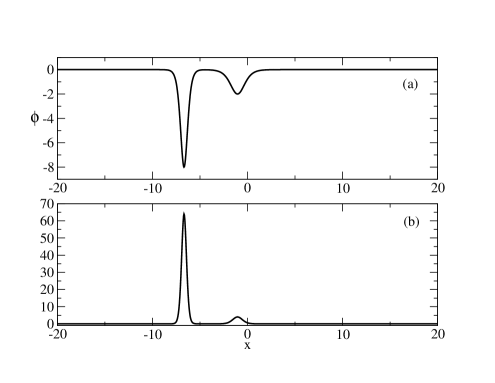
Figure 7: The bisoliton solution to Equation (127). (a) The bisoliton solution of the Korteweg–de Vries equation. (b) The corresponding bisoliton solution of (127). The parameters of the solution are $c=2.0$, $\alpha=1/2$.

The soliton properties of the solution (130) are illustrated in Figure 8. We observe the motion of two solitons having different velocities. The larger (and the faster) soliton moves through the smaller soliton and continues to travel without change in its form. The smaller soliton also does not change its form.

Figure 8: Illustration of the soliton properties of the waves connected to the bisoliton solution of (127). The parameters of the solution are $c=3.2$, $\alpha=1/2$.

Proposition 26.

The equation

$$\frac{\partial\phi}{\partial t}+\left(\frac{\partial\phi}{\partial x}\right)^{3}+3\frac{\partial\phi}{\partial x}+\frac{\partial^{3}\phi}{\partial x^{3}}-6\exp(\phi)\frac{\partial\phi}{\partial x}=0,$$ (131)

has the solutions

$$\phi(x,t)=\ln\left\{-\frac{c}{2}{\rm sech}^{2}\left[\frac{\sqrt{c}}{2}(x-ct)\right]\right\},$$ (132)

and

$$\phi(x,t)=\ln\left\{-2\frac{\partial^{2}}{\partial x^{2}}\ln\det[A(x,t)]\right\},$$ (133)

and

$$u(x,t)=\ln\left\{-12\frac{3+4\cosh(8t-2x)+\cosh(64t-4x)}{[\cosh(36t-3x)+3\cosh(28t-x)]^{2}}\right\}.$$ (134)

Proof.

We apply the transformation $u=\exp(\phi)$ to Equation (123). The transformation transforms (123) to (131). The solutions (124), (125) and (126) are transformed to (132), (133) and (134). ∎

Proposition 27.

The equation

$$\phi^{2}\frac{\partial\phi}{\partial t}+\phi^{2}\frac{\partial^{3}\phi}{\partial x^{3}}-3\phi\frac{\partial\phi}{\partial x}\frac{\partial^{3}\phi}{\partial x^{3}}+2\left(\frac{\partial\phi}{\partial x}\right)^{3}-6\ln(\phi)\phi\left(\frac{\partial\phi}{\partial x}\right)^{2}=0,$$ (135)

has the solutions

$$\phi(x,t)=\exp\left\{-\frac{c}{2}{\rm sech}^{2}\left[\frac{\sqrt{c}}{2}(x-ct)\right]\right\},$$ (136)

and

$$\phi(x,t)=\exp\left\{-2\frac{\partial^{2}}{\partial x^{2}}\ln\det[A(x,t)]\right\},$$ (137)

and

$$\phi(x,t)=\exp\left\{-12\frac{3+4\cosh(8t-2x)+\cosh(64t-4x)}{[\cosh(36t-3x)+3\cosh(28t-x)]^{2}}\right\}.$$ (138)

Proof.

We apply the transformation $u=\ln(\phi)$ to Equation (123). The transformation transforms (123) to (135). The solutions (124), (125) and (126) are transformed to (136), (137) and (138). ∎

Figure 9 illustrates the soliton and the bisoliton solution to Equation (135).

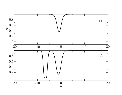
Figure 9: The soliton and the bisoliton solution to Equation (135). (a) The soliton solution. (b) The corresponding bisoliton solution of (135).

5 Concluding Remarks

Transformations are very useful for obtaining exact solutions of nonlinear differential equations. As examples, we mention the Bäcklund transformation [60]-[71] and the transformation of Darboux [72]-[81]. The transformation of Bäcklund allows us to obtain new exact solutions of appropriate equation if we know an exact solution of this equation. The Darboux transformation is a simultaneous mapping between solutions and coefficients to a pair of equations (or systems of equations) of the same form. The methodology proposed in this article allows us to obtain exact solutions to nonlinear differential equations if we know exact solutions of different (linear or nonlinear) differential equations.

In this article, we study the possibility of obtaining exact solutions to nonlinear differential equations by means of transformations applied to more simple (linear or nonlinear) differential equations. The idea of this method of transformations is very simple: a transformation transforms a linear or nonlinear differential equation with a known solution to a more complicated nonlinear differential equation. The same transformation transforms the known solution of the more simple equation to an exact solution to the corresponding nonlinear equation. A similar idea, for example, is used in the simple equations method (SEsM). There, we have a simple equation which usually is a nonlinear differential equation with a known solution. By means of this solution, we construct a solution of a more complicated nonlinear differential equation. This construction can be thought of as a transformation which transforms the solution of the simple equation to the solution of the more complicated equation.

In this article, we demonstrate the result of the application of very simple transformations on several linear and nonlinear differential equations. We obtain solutions of nonlinear differential equations which are connected to interesting phenomena: (a) occurrence of a solitary wave–solitary antiwave from a state which is equal to $0$ at the moment $t=0$; (b) splitting of solitary wave of two solitary waves; (c) solitons which have different amplitude and the same velocity. We stress result (c). Usually, solitons of different heights have different velocities. This can be observed in Figure 8. There, the larger (and the faster) soliton passes through the smaller (and the slower) soliton and continues to travel without change in its form. Figure 6 shows that we can have two solitons of different forms which travel with the same velocity. We observe the collision of these solitons and after the collision they travel further without change in their form. Such a possible class of solitons is very interesting.

One limitation of the discussed methodology is that it needs an equation with a known exact solution in order to obtain exact solutions of other equations. This limitation is the same as in the case of other transformation methodologies such as, for example, the methodology based on the Bäcklund transformation. Another limitation of the methodology is that we need to know not only the transformation $u=u(\phi,\dots)$, but also the explicit form of the inverse transformation $\phi=\phi(u,\dots)$ in order to construct the exact solution of the equation for $\phi$.

The methodology reported in this article can be applied to various problems. First of all, one can study additional equations. Just one example is the class of equations connected to the nonlinear Schrödinger equation. Let us consider the equation [82]

$$i\frac{\partial u}{\partial t}+\frac{\partial^{2}u}{\partial x^{2}}+\kappa\mid u\mid^{2}u=0,$$ (139)

where $\kappa$ is a parameter. This equation has the multisoliton solutions

$$\mid u(x,t)\mid^{2}=(2\kappa)^{1/2}\frac{d^{2}}{dx^{2}}\ln\det\mid\mid BB^{*}+1\mid\mid.$$ (140)

The notation ^∗ means complex conjugation. The matrix $B$ from (140) is

$$B_{jk}=\frac{(c_{j}c_{k}^{*})^{1/2}}{\zeta_{j}-\zeta_{k}^{*}}\exp[i(\zeta_{j}-\zeta_{k}^{*})x];\ \ \ c_{j}(t)=c_{j}(0)\exp(4i\zeta^{2}t).$$ (141)

In (141) $\zeta=\frac{\lambda p}{1-p^{2}}$, where $p$ is determined from $\kappa=\frac{2}{1-p^{2}}$, $\zeta_{i}$ are the eigenvalues of problem (8) from [82] and $\lambda$ is the eigenvalue from (7) of [82], where $\hat{L}$ is operator (5) from [82].

The transformation $u=u(\phi)$ transforms the nonlinear Schrödinger equation to

$$i\frac{du}{d\phi}\frac{\partial\phi}{\partial t}+\frac{d^{2}u}{d\phi^{2}}\left(\frac{\partial\phi}{\partial x}\right)^{2}+\frac{du}{d\phi}\frac{\partial^{2}\phi}{\partial x^{2}}+\kappa\mid u^{2}\mid u=0.$$ (142)

Let us specify the form of the transformation to $u=\phi^{\alpha}$, where $\alpha$ is a constant and $\alpha\neq 1$. Equation (142) is reduced to

$$i\alpha\phi\frac{\partial\phi}{\partial t}+\alpha(\alpha-1)\left(\frac{\partial\phi}{\partial x}\right)^{2}+\alpha\phi\frac{\partial^{2}\phi}{\partial x^{2}}+\kappa\phi^{2}\mid\phi\mid^{2\alpha}=0.$$ (143)

The multisoliton solution of (143) is $\phi=u^{1/\alpha}$, where $u$ is given by (140).

Another possible direction for the extension of the reported research is to apply more complicated transformations and this will lead to exact solutions of even more complicated nonlinear differential equations. Moreover, the stability of the obtained solutions can be studied as in [82]. The results of such kinds of research will be reported elsewhere.

Appendix A Linear Differential Equations and Their Solutions Used in the Main Text

In the main text, we discuss the following linear differential equations and their solutions.

1. The hyperbolic equation

$$c^{2}\frac{\partial^{2}u}{\partial x^{2}}-\frac{\partial^{2}u}{\partial t^{2}}=0,$$ (144)

where $-\infty\leq a<x<b\leq+\infty$, and $t>0$. This is the (1+1)-D wave equation. We consider the general solution

$$u(x,t)=F(x+ct)+G(x-ct),$$ (145)

where $F$ and $G$ are arbitrary $C^{2}$-functions. In addition, we consider the Cauchy problem

$$u(x,0)=f(x),\ \ \ \frac{\partial u}{\partial t}(x,0)=g(x),\ \ -\infty<x<\infty,t>0.$$ (146)

The solution of this problem is given by d’Alembert’s formula

$$u(x,t)=\frac{f(x+ct)+f(x-ct)}{2}+\frac{1}{2c}\int\limits_{x-ct}^{x+ct}ds\ g(s).$$ (147)

Finally, we will use the solution for the case $0<x<L$ and initial and boundary conditions

$$u(x,0)=f(x),\ \ \ \frac{\partial u}{\partial t}(x,0)=g(x),\ \ 0\leq x\leq L,$$

$$\frac{\partial u}{\partial x}(0,t)=\frac{\partial u}{\partial x}(L,t)=0,\ \ t\geq 0.$$ (148)

The solution in this case is

$$u(x,t)=\sum\limits_{n=1}^{\infty}\Bigg{[}a_{n}\cos\Bigg{(}\frac{n\pi ct}{L}\Bigg{)}+b_{n}\sin\Bigg{(}\frac{n\pi ct}{L}\Bigg{)}\Bigg{]}\sin\Bigg{(}\frac{n\pi x}{L}\Bigg{)},$$

$$a_{n}=\frac{2}{L}\int\limits_{0}^{L}dx\ f(x)\sin\Bigg{(}\frac{n\pi x}{L}\Bigg{)},\ \ \ b_{n}=\frac{2}{n\pi c}\int\limits_{0}^{L}dx\ g(x)\sin\Bigg{(}\frac{n\pi x}{L}\Bigg{)}.$$ (149)

2. The parabolic equation

$$a^{2}\frac{\partial^{2}u}{\partial x^{2}}-\frac{\partial u}{\partial t}=0.$$ (150)

This is the (1 + 1)-D heat equation. For the case $-\infty<x<\infty$ and for the initial condition $u(x,0)=f(x)$, solution is given by the integral of Poisson

$$u(x,t)=\frac{1}{2a\sqrt{\pi t}}\int\limits_{-\infty}^{+\infty}d\xi\ f(\xi)\exp\left[-\frac{(\xi-x)^{2}}{4at^{2}}\right].$$ (151)

For the case $0<x<L$ and initial and boundary conditions $u(x,0)=f(x)$ and $u(0,t)=A$, $u(L,t)=B$, the solution is

$$u(x,t)=A+\frac{B-A}{L}+\sum\limits_{n=1}^{\infty}a_{n}\exp\Bigg{(}-\frac{\pi^{2}a^{2}n^{2}}{L^{2}}t\Bigg{)}\sin\Bigg{(}\frac{n\pi x}{L}\Bigg{)},$$

$$a_{n}=-\frac{2}{n\pi}[A+(-1)^{n+1}B]+\frac{2}{L}\int\limits_{0}^{L}dx\ f(x)\sin\Bigg{(}\frac{n\pi x}{L}\Bigg{)}.$$ (152)

3. The elliptic equation

$$\frac{\partial^{2}u}{\partial x^{2}}+\frac{\partial^{2}u}{\partial y^{2}}=0.$$ (153)

This is the 2D Laplace equation. Here, we consider only the solution for the case of the rectangle domain $a<x<b$, $c<x<d$ and boundary conditions $u(a,y)=f(y)$; $u(b,y)=g(y)$; $u(x,c)=h(c)$; $u(x,d)=k(x)$. The solution is

$$u=u_{1}+u_{2};\ \ \ u_{1}=\sum\limits_{n}X_{n}(x)Y_{n}(y);\ \ \ u_{2}=\sum\limits_{m}Z_{m}(x)V_{m}(y),$$ (154)

where the boundary conditions for $u_{1,2}$ are $u_{1}(a,y)=f(y),u_{1}(b,y)=g(y),u_{1}(x,c)=0,u-1(x,d)=0$; $u_{2}(a,y)=0,u_{2}(b,y)=0,u_{2}(x,c)=h(x),u_{2}(x,d)=k(x)$, where $X_{n},Y_{n},Z_{m},V_{m}$ are solutions of the equations

$$\frac{d^{2}X}{dx}-\lambda_{1}X(x)=0,\ a<x<b,$$

$$\frac{d^{2}Y}{dy}-\lambda_{2}Y(y)=0,\ c<y<d,$$

$$\frac{d^{2}Z}{dx}-\lambda_{3}Z(x)=0,\ a<x<b,$$ (155)

$$\frac{d^{2}V}{dy}-\lambda_{4}V(y)=0,\ c<y<d.$$

References

- [1] Latora, V.; Nicosia, V.; Russo, G. Complex Networks. Principles, Methods, and Applications; Cambridge University Press: Cambridge, UK, 2017; ISBN 978-1-107-10318-4.
- [2] Vitanov, N.K. Science Dynamics and Research Production. Indicators, Indexes, Statistical Laws and Mathematical Models; Springer: Cham, Switzerland, 2016; ISBN 978-3-319-41629-8.
- [3] Treiber, M.; Kesting, A. Traffic Flow Dynamics: Data, Models, and Simulation; Springer: Berlin/Heidelberg, Germany, 2013; ISBN 978-3-642-32460-4.
- [4] Dimitrova, Z.I. Flows of Substances in Networks and Network Channels: Selected Results and Applications. Entropy 2022, 24, 1485. https://doi.org/10.3390/e24101485.
- [5] Drazin, P.G. Nonlinear Systems; Cambridge University Press: Cambridge, UK, 1992; ISBN 0-521-40489-4.
- [6] Kantz, H.; Schreiber, T. Nonlinear Time Series Analysis; Cambridge University Press: Cambridge, UK, 2004; ISBN 978-0511755798.
- [7] Verhulst, F. Nonlinear Differential Equations and Dynamical Systems; Springer: Berlin/Heidelberg, Germany, 2006; ISBN 978-3-540-60934-6.
- [8] Popivanov, P.; Slavova, A. Nonlinear Waves: An Introduction; World Scientific: Singapore, 2010; ISBN 9789813107953.
- [9] Debnath, L. (Eds.) Nonlinear Waves; Cambridge University Press: Cambridge, UK, 1983; ISBN 0-521-25468-X.
- [10] Kulikovskiii, A.; Sveshnikova, E. Nonlinear Waves in Elastic Media; CRC Press: Boca Raton, FL, USA, 2021; ISBN 0-8493-8643-8.
- [11] Ma, Q. Advances in Numerical Simulation of Nonlinear Water Waves; World Scientific: Singapore, 2010; ISBN 9789812836502.
- [12] Osborne, A.R. Nonlinear Topics in Ocean Physics; North-Holland: Amsterdam, The Netherlands, 1991; ISBN 9780444597823.
- [13] Nazarov, V.; Radostin, A. Nonlinear Acoustic Waves in Micro-Inhomogeneous Solids; Wiley: Chchester, UK, 2005; ISBN 9781118456088.
- [14] Kim, C.-H. Nonlinear Waves and Offshore Structures; World Scientific: Singapore, 2008; ISBN 9789813102484.
- [15] Fillipov, A.T. The Versatile Soliton; Springer: New York, 2010; ISBN 9780817649746.
- [16] Akhmediev, N.; Ankiewicz, A. Dissipative Solitons; Springer: Berlin, Germany, 2005, ISBN 9783540233732.
- [17] Davydov, A.S. Solitons in Molecular Systems; Springer: Dordrecht, The Netherlands, 2013; ISBN 9789401730259.
- [18] Olver, P.J.; Sattiger, D.H. Solitons in Physics, Mathematics, and Nonlinear Optics; Springer: New York, NY, USA, 2012; ISBN 9781461390336.
- [19] Ablowitz, M.J.; Clarkson, P.A. Solitons, Nonlinear Evolution Equations and Inverse Scattering; Cambridge University Press: Cambridge, UK, 1991; ISBN 978-0511623998.
- [20] Ablowitz, M. J.; Kaup, D. J.; Newell, A. C.; Segur, H. The Inverse Scattering Transform‐Fourier Analysis for Nonlinear Problems. Studies in Applied Mathematics, 1974, 53 (4), 249 – 315. https://doi.org/10.1002/sapm1974534249
- [21] Ablowitz, M. J.; Musslimani, Z. H. Inverse Scattering Transform for the Integrable Nonlocal Nonlinear Schrödinger Equation. Nonlinearity, 2016, 29 (3), 915. https://doi.org/10.1088/0951-7715/29/3/915
- [22] Vitanov, N. K. Simple Equations Method (SEsM) and its Connection with the Inverse Scattering Transform Method. AIP Conference Proceedings 2021, 2321, 030035, https://doi.org/10.1063/5.0040409
- [23] Fokas, A. S.; Ablowitz, M. J. The Inverse Scattering Transform for the Benjamin‐Ono Equation—A Pivot to Multidimensional Problems. Studies in Applied Mathematics, 1983, 68 (1), 1-10. https://doi.org/10.1002/sapm19836811
- [24] Zhang, X.; Chen, Y. Inverse Scattering Transformation for Generalized Nonlinear Schrödinger Equation. Applied Mathematics Letters, 2019, 98, 306 – 313. https://doi.org/10.1016/j.aml.2019.06.014
- [25] Osborne, A. R. The Inverse Scattering Transform: Tools for the Nonlinear Fourier Analysis and Filtering of Ocean Surface Waves. Chaos, Solitons & Fractals, 1995 5 (12), 2623 – 2637. https://doi.org/10.1016/0960-0779(94)E0118-9
- [26] Osborne, A. R. Soliton Physics and the Periodic Inverse Scattering Transform. Physica D,1995, 86 (1-2), 81 – 89. https://doi.org/10.1016/0167-2789(95)00089-M
- [27] Ji, J. L.; Zhu, Z. N. Soliton Solutions of an Integrable Nonlocal Modified Korteweg–de Vries Equation Through Inverse Scattering Transform. Journal of Mathematical Analysis and Applications, 2017, 453(2), 973 – 984. https://doi.org/10.1016/j.jmaa.2017.04.042
- [28] Hirota, R. The Direct Method in Soliton Theory; Cambridge University Press: Cambridge, UK, 2004; ISBN 0-521-83660-3.
- [29] Gibbon, J. D.; Radmore, P.; Tabor, M.; Wood, D. The Painleve Property and Hirota’s Method. Studies in Applied Mathematics, 1985, 72 (1), 39 – 63. https://doi.org/10.1002/sapm198572139
- [30] Gürses, M.; Pekcan, A. Nonlocal Modified KdV Equations and Their Soliton Solutions by Hirota Method. Communications in Nonlinear Science and Numerical Simulation, 2019, 67, 427-448. https://doi.org/10.1016/j.cnsns.2018.07.013
- [31] Zhou, Y.; Ma, W. X. Complexiton Solutions to Soliton Equations by the Hirota Method. Journal of Mathematical Physics, 2017, 58 (10). https://doi.org/10.1063/1.4996358
- [32] Jia, T. T.; Chai, Y. Z.; Hao, H. Q. Multi-soliton Solutions and Breathers for the Generalized Coupled Nonlinear Hirota Equations via the Hirota Method. Superlattices and Microstructures, 2017, 105, 172-182. https://doi.org/10.1016/j.spmi.2016.10.091
- [33] Ma, W. X. Soliton Solutions by Means of Hirota Bilinear Forms. Partial Differential Equations in Applied Mathematics, 2022, 5, 100220. https://doi.org/10.1016/j.padiff.2021.100220
- [34] Infeld, E.; Rowlands, G. Nonlinear Waves, Solitons and Chaos; Cambridge University Press: Cambridge, UK, 2000; ISBN 0-521-63212-9.
- [35] Zhao, Z.-L.; He, L.-C.; Wazwaz, A.-M. Dynamics of Lump Chains for the BKP Equation Describing Propagation of Nonlinear Wave. Chin. Phys. B 2023, 32, 040501. https://doi.org/10.1088/1674-1056/acb0c1.
- [36] Ablowitz, M.J. Nonlinear Dispersive Waves: Asymptotic Analysis and Solitons; Cambridge University Press: Cambridge, UK, 2011; ISBN 9781107012547.
- [37] Calogero, F.; Degasperis, A. Spectral Transform and Solitons; North Holland: Amsterdam, The Netherlands, 1982; ISBN 0-444-86368-0.
- [38] Osborne, A.R.; Bergamasco, L. The Solitons of Zabusky and Kruskal revisited: Perspective in Terms of the Periodic Spectral Transform. Physica D 1986, 18, 26–46. https://doi.org/10.1016/0167-2789(86)90160-0.
- [39] Wadati, M.; Sogo, K. Gauge Transformations in Soliton theory. J. Phys. Soc. Jpn. 1983, 52, 394–398. https://doi.org/10.1143/JPSJ.52.394.
- [40] Buccoliero, D.; Desyatnikov, A.S. Quasi-periodic Transformations of Nonlocal Spatial Solitons. Opt. Express 2009, 17, 9608–9613. https://doi.org/10.1364/OE.17.009608.
- [41] Date, E.; Jimbo, M.; Kashiwara, M.; Miwa, T. Transformation Groups for Soliton Equations: IV. A New Hierarchy of Soliton Equations of KP-type. Physica D 1982, 4, 343–365. https://doi.org/10.1016/0167-2789(82)90041-0.
- [42] Whitham, G.B.; Linear and Nonlinear Waves; Wiley: New York, NY, USA, 1999; ISBN 0-471-35942-4.
- [43] Zakharov, V.E.; Wabnitz, S. (Eds.) Optical Solitons: Theoretical Challenges and Industrial Perspectives; Springer: Berlin/Heidelberg, Germany, 2013; ISBN 9783662038079.
- [44] Gibbon, J.D. A Survey of the Origins and Physical Importance of Soliton Equations. Philos. Trans. R. Soc. Lond. Ser. A Math. Phys. Sci. 1985, 315, 335–365.
- [45] Ur Rehman, H.; Awan, A.U.; Habib, A.; Gamaoun, F.; El Din, M.T.; Galal, A.M. Solitary Wave Solutions for a Strain Wave Equation in a microstructured Solid. Results Phys. 2022, 39, 105755. https://doi.org/10.1016/j.rinp.2022.105755.
- [46] Newell, A.C. The General Structure of Integrable Evolution Equations. Proc. R. Soc. Lond. A Math. Phys. Sci. 1979, 365, 283–311. https://doi.org/10.1098/rspa.1979.0018.
- [47] Yang, J. Nonlinear Waves in Integrable and Nonintegrable Systems; SIAM: Philadelphia, PA, USA, 2010; ISBN 9780898719680.
- [48] Rogers, C.; Schief, W.K. Bäcklund and Darboux Transformations: Geometry and Modern Applications in Soliton Theory; Cambridge University Press: Cambridge, UK, 2002; ISBN 9780521012881.
- [49] Vitanov, N.K. Simple Equations Method (SEsM): An Effective Algorithm for Obtaining Exact Solutions of Nonlinear Differential Equations. Entropy 2022, 24, 1653. https://doi.org/10.3390/e24111653.
- [50] Vitanov, N.K.; Dimitrova, Z.I.; Vitanov, K.N. Simple Equations Method (SEsM): Algorithm, Connection with Hirota Method, Inverse Scattering Transform Method, and Several Other Methods. Entropy 2021, 23, 10. https://doi.org/10.3390/e23010010.
- [51] Vitanov, N.K.; Dimitrova, Z.I. Simple Equations Method and Non-linear Differential Equations with Non-polynomial Non-linearity. Entropy 2021, 23, 1624. https://doi.org/10.3390/e23121624.
- [52] Vitanov, N.K.; Dimitrova, Z.I.; Vitanov, K.N. On the Use of Composite Functions in the Simple Equations Method to Obtain Exact Solutions of Nonlinear Differential Equations. Computation 2021, 9, 104. https://doi.org/10.3390/computation9100104.
- [53] Vitanov, N. K.; Dimitrova, Z.I. Modified Method of Simplest equation Applied to the Nonlinear Schrödinger Equation. Journal of Theoretical and Applied Mechanics, 2018, 48 (1), 59 – 69. https://doi.org/10.2478/jtam-2018-0005
- [54] Vitanov, N. K. Modified Method of Simplest Equation: Powerful tool for Obtaining Exact and approximate Traveling-wave solutions of Nonlinear PDEs. Communications in Nonlinear Science and Numerical Simulation, 2011, 16 (3), 1176 – 1185. https://doi.org/10.1016/j.cnsns.2010.06.011
- [55] Vitanov, N. K.; Dimitrova, Z. I.; Kantz, H. (2010). Modified Method of Simplest equation and its Application to Nonlinear PDEs. Applied Mathematics and Computation, 2010, 216 (9), 2587 – 2595. https://doi.org/10.1016/j.amc.2010.03.102
- [56] Vitanov, N. K. On Modified Method of Simplest Equation for Obtaining Exact and Approximate Solutions of Nonlinear PDEs: The role of the Simplest Equation. Communications in Nonlinear Science and Numerical Simulation, 2011, 16 (11), 4215 – 4231. https://doi.org/10.1016/j.cnsns.2011.03.035
- [57] Vitanov, N. K.; Dimitrova, Z. I.; Vitanov, K. N. Modified Method of Simplest Equation for Obtaining Exact Analytical Solutions of Nonlinear Partial Differential Equations: Further development of the Methodology with Applications. Applied Mathematics and Computation, 2015, 269, 363 – 378. https://doi.org/10.1016/j.amc.2015.07.060
- [58] Hopf, E. The Partial Differential Equation: . Commun. Pure Appl. Math. 1950, 3, 201–230. https://doi.org/10.1002/cpa.3160030302.
- [59] Cole, J.D. On a Quasi-Linear Parabolic Equation Occurring in Aerodynamics. Q. Appl. Math. 1951, 9, 225–236. https://doi.org/10.1090/qam/42889.
- [60] Wahlquist, H.D.; Estabrook, F.B. Bäcklund Transformation for Solutions of the Korteweg-de Vries Equation. Phys. Rev. Lett. 1973 31, 1386–1390. https://doi.org/10.1103/PhysRevLett.31.1386.
- [61] Dodd, R.K.; Bullough, R.K. Bäcklund Transformations for the Sine–Gordon Equations. Proc. R. Soc. Lond. A 1976, 351, 499–523. https://doi.org/10.1098/rspa.1976.0154.
- [62] Satsuma, J.; Kaup, D.J. A Bäcklund Transformation for a Higher Order Korteweg-de Vries Equation. J. Phys. Soc. Jpn. 1977, 43, 692–697. https://doi.org/10.1143/JPSJ.43.692.
- [63] Hirota, R.; Satsuma, J. A Variety of Nonlinear Network Equations Generated from the Bäcklund Transformation for the Toda Lattice. Prog. Theor. Phys. Suppl. 1976, 59, 64–100. https://doi.org/10.1143/PTPS.59.64.
- [64] Gao, X.Y.; Guo, Y.J.; Shan, W.R. Regarding the Shallow Water in an Ocean via a Whitham-Broer-Kaup-like System: Hetero-Bäcklund Transformations, Bilinear Forms and M Solitons. Chaos Solitons Fractals 2022, 162, 112486. https://doi.org/10.1016/j.chaos.2022.112486.
- [65] Hirota, R. A New Form of Bäcklund Transformations and its Relation to the Inverse Scattering Problem. Progress of Theoretical Physics, 1974, 52(5), 1498 – 1512. https://doi.org/10.1143/PTP.52.1498
- [66] Lamb Jr, G. L. Bäcklund Transformations for Certain Nonlinear Evolution Equations. Journal of Mathematical Physics, 1974, 15 (12), 2157 – 2165. https://doi.org/10.1063/1.1666595
- [67] Fan, E. Auto-Bäcklund Transformation and Similarity Reductions for General Variable Coefficient KdV Equations. Physics Letters A,2002, 294 (1), 26 – 30. https://doi.org/10.1016/S0375-9601(02)00033-6
- [68] Zhou, T. Y.; Tian, B.; Chen, S. S.; Wei, C. C.; Chen, Y. Q. Bäcklund Transformations, Lax pair and Solutions of a Sharma-Tasso-Olver-Burgers Equation for the Nonlinear Dispersive Waves. Modern Physics Letters B, 2021, 35 (35), 2150421. https://doi.org/10.1142/S0217984921504212
- [69] Wang, G.; Liu, Q. P.; Mao, H. The Modified Camassa–Holm eEquation: Bäcklund Transformation and Nonlinear Superposition Formula. Journal of Physics A: Mathematical and Theoretical, 2020, 53 (29), 294003. https://doi.org/10.1088/1751-8121/ab7136
- [70] Gao, X. Y.; Guo, Y. J.; Shan, W. R. Bilinear Forms through the Binary Bell Polynomials, N Solitons and Bäcklund Transformations of the Boussinesq– Burgers System for the Shallow Water Waves in a Lake or Near an Ocean Beach. Communications in Theoretical Physics, 2020, 72 (9), 095002. https://doi.org/10.1088/1572-9494/aba23d
- [71] Wang, K.J. Bäcklund Transformation and Diverse Exact Explicit Solutions of the Fractal Combined Kdv–mkdv Equation. Fractals 2022, 30, 2250189. https://doi.org/10.1142/S0218348X22501894.
- [72] Guo, B.; Ling, L.; Liu, Q.P. Nonlinear Schrödinger Equation: Generalized Darboux Transformation and Rogue Wave Solutions. Phys. Rev. E 2012, 85, 026607. https://doi.org/10.1103/PhysRevE.85.026607.
- [73] Xu, S.; He, J.; Wang, L. The Darboux Transformation of the Derivative Nonlinear Schrödinger Equation. J. Phys. A Math. Theor. 2011, 44, 305203. https://doi.org/10.1088/1751-8113/44/30/305203.
- [74] Gu, C.; Hu, H.; Zhou, Z. Darboux Transformations in Integrable Systems: Theory and their Applications to Geometry. Springer: Dordrecht, 2005; ISBN 1-4020-3087-8
- [75] Gu, C.; Hu, H.; Zhou, Z. Darboux Transformations in Integrable Systems: Theory and Their Applications to Geometry; Springer Science & Business Media: Dordrecht, The Netherlands, 2005; ISBN 1-4020-3087-8.
- [76] Li, Y.; Zhang, J. E. Darboux Transformations of Classical Boussinesq system and its Multi-soliton Solutions. Physics Letters A, 2001, 284 (6), 253 – 258. https://doi.org/10.1016/S0375-9601(01)00331-0
- [77] Ma, W. X.; Zhang, Y. J. Darboux Transformations of Integrable Couplings and Applications. Reviews in Mathematical Physics, 2018, 30(02), 1850003. https://doi.org/10.1142/S0129055X18500034
- [78] Aktosun, T.; Van der Mee, C. A Unified Approach to Darboux Transformations. Inverse Problems, 2009, 25 (10), 105003. https://doi.org/10.1088/0266-5611/25/10/105003
- [79] Xu, S.; He, J.; Wang, L. The Darboux Transformation of the Derivative Nonlinear Schrödinger equation. Journal of Physics A: Mathematical and Theoretical, 2011, 44 (30), 305203. https://doi.org/10.1088/1751-8113/44/30/305203
- [80] Qiu, D.; He, J.; Zhang, Y.; Porsezian, K. The Darboux Transformation of the Kundu–Eckhaus Equation. Proceedings of the Royal Society A, 2015, 471 (2180), 20150236. https://doi.org/10.1098/rspa.2015.0236
- [81] Matveev, V. B. Darboux Transformation and Explicit solutions of the Kadomtcev-Petviaschvily equation, depending on Functional Parameters. Letters in Mathematical Physics, 1979, 3, 213 – 216. https://doi.org/10.1007/BF00405295
- [82] Zakharov, V.E.; Shabat, A.V. Exact Theory of Two-dimensional Self-Focusing and One-dimensional Self-modulation of Waves in Nonlinear Media. Sov. Phys. JETP 1972, 34, 62–69.