Grand-Clément, Petrik and Vieille Robust MDPs with average and Blackwell optimality Beyond discounted returns: Robust Markov decision processes with average and Blackwell optimality Julien Grand-Clément Information Systems and Operations Management Department, HEC Paris, grand-clement@hec.fr Marek Petrik Department of Computer Science, University of New Hampshire, mpetrik@cs.unh.edu Nicolas Vieille Economics and Decision Sciences Department, HEC Paris, vieille@hec.fr Robust Markov Decision Processes (RMDPs) are a widely used framework for sequential decision-making under parameter uncertainty. RMDPs have been extensively studied when the objective is to maximize the discounted return, but little is known for average optimality (optimizing the long-run average of the rewards obtained over time) and Blackwell optimality (remaining discount optimal for all discount factors sufficiently close to $1$). In this paper, we prove several foundational results for RMDPs beyond the discounted return. We show that average optimal policies can be chosen stationary and deterministic for sa-rectangular RMDPs but, perhaps surprisingly, that history-dependent (Markovian) policies strictly outperform stationary policies for average optimality in s-rectangular RMDPs. We also study Blackwell optimality for sa-rectangular RMDPs, where we show that approximate Blackwell optimal policies always exist, although Blackwell optimal policies may not exist. We also provide a sufficient condition for their existence, which encompasses virtually any examples from the literature. We then discuss the connection between average and Blackwell optimality, and we describe several algorithms to compute the optimal average return. Interestingly, our approach leverages the connections between RMDPs and stochastic games. Robust Markov decision process, average optimality, Blackwell optimality, value iteration

1 Introduction

Markov decision process (MDP) (Puterman, 2014) is one of the most popular frameworks to model sequential decision-making by a single agent, with recent applications to game solving and reinforcement learning (Sutton and Barto, 2018; Mnih et al., 2013), healthcare decision-making (Bennett and Hauser, 2013; Steimle and Denton, 2017) and finance (Bäuerle and Rieder, 2011). Robust Markov decision processes (RMDPs) is a generalization of MDPs, dating as far back as Satia and Lave (1973) and extensively studied more recently after the seminal papers of Iyengar (2005) and Nilim and Ghaoui (2005). Robust MDPs consider a single agent repeatedly interacting with an environment with unknown instantaneous rewards and/or transition probabilities. The unknown parameters are assumed to be chosen adversarially from an uncertainty set, modeling the set of all plausible values of the parameters.

Most of the robust MDP literature has focused on computational and algorithmic considerations for the discounted return, where the future instantaneous rewards are discounted with a discount factor $\gamma\in(0,1)$. In this case, RMDPs become tractable under certain rectangularity assumptions, with models such as sa-rectangularity (Iyengar, 2005; Nilim and Ghaoui, 2005), s-rectangularity (Le Tallec, 2007; Wiesemann et al., 2013), k-rectangularity (Mannor et al., 2016), and r-rectangularity (Goh et al., 2018; Goyal and Grand-Clément, 2022). For rectangular RMDPs, iterative algorithms can be efficiently implemented for various distance- and divergence-based uncertainty sets (Givan et al., 1997; Iyengar, 2005; Ho et al., 2021; Grand-Clement and Kroer, 2021; Behzadian et al., 2021), as well as gradient-based algorithms (Wang et al., 2022; Kumar et al., 2023; Li et al., 2022, 2023).

Robust MDPs have found some applications in healthcare (Zhang et al., 2017; Goh et al., 2018; Grand-Clément et al., 2023), where the set of states represents the potential health conditions of the patients, actions represent the medical interventions, and it is critical to account for the potential errors in the estimated transition probabilities representing the evolution of the patient’s health, and in inverse reinforcement learning (Viano et al., 2021; Chae et al., 2022) for imitations that are robust to shifts between the learner’s and the experts’ dynamics. In some applications, introducing a discount factor can be seen as a modeling choice, e.g. in finance (Deng et al., 2016). In other applications like game-solving (Mnih et al., 2013; Brockman et al., 2016), the discount factor is merely introduced for algorithmic purposes, typically to ensure the convergence of iterative algorithms or to reduce variance (Baxter and Bartlett, 2001), and it may not have any natural interpretation. Additionally, large discount factors may slow the convergence rate of the algorithms. Average optimality, i.e., optimizing the limit of the average of the instantaneous rewards obtained over an infinite horizon, and Blackwell optimality, i.e., finding policies that remain discount optimal for all discount factors sufficiently close to $1$, provide useful objective criteria for environments with no natural discount factor, unknown discount factor, or large discount factor. To the best of our knowledge, the literature on robust MDPs that address these optimality notions is scarce. The authors in Tewari and Bartlett (2007); Wang et al. (2023) study RMDPs with the average return criterion but only focus on computing the optimal worst-case average returns among stationary policies, without any guarantee that average optimal policies may be chosen in this class of policies. Similarly, some previous papers show the existence of Blackwell optimal policies for sa-rectangular RMDPs, but they require some restrictive assumptions, such as polyhedral uncertainty sets (Tewari and Bartlett, 2007; Goyal and Grand-Clément, 2022) or unichain RMDPs with a unique average optimal policy (Wang et al., 2023).

Our goal in this paper is to study RMDPs with average and Blackwell optimality in the general case. Our main contributions can be summarized as follows.

1. Average optimality. For sa-rectangular robust MDPs with compact convex uncertainty sets, we show the existence of a stationary deterministic policy that is average optimal, thus closing an important gap in the literature. Additionally, we describe several strong duality results and we highlight that the worst-case transition probabilities need not exist, a fact that has been overlooked by previous work. We also discuss the case of robustness against history-dependent worst-case transition probabilities. In addition, we show for s-rectangular RMDPs that surprisingly, stationary policies may be suboptimal for the average return criterion. That is, history-dependent (Markovian) policies may be necessary to achieve the optimal average return.

2. Blackwell optimality. We provide an extensive treatment of Blackwell optimality for sa-rectangular RMDPs. In this case, we provide a counterexample where Blackwell optimal policies fail to exist, and we identify the pathological oscillating behaviors of the robust value functions as the key factor for this non-existence. We show however that approximate Blackwell optimal policies always exist. Finally, we introduce the notion of definable uncertainty sets, which are sets built on simple enough functions to ensure that the discounted value functions are “well-behaved”. The definability assumption captures virtually all uncertainty sets used in practice for sa-rectangular RMDPs, and we show that for sa-rectangular RMDPs with definable uncertainty sets, there always exists a stationary deterministic policy that is Blackwell optimal. We also highlight the connections between Blackwell optimal policies and average optimal policies. For s-rectangular RMDPs, we provide a simple example where Blackwell optimal policies do not exist, even in the simple case of polyhedral uncertainty.

3. Algorithms and numerical experiments. We introduce three algorithms that converge to the optimal average return, in the case of definable sa-rectangular uncertainty sets. We note that efficiently computing an average optimal policy for sa-rectangular RMDPs is a long-standing open problem in algorithmic game theory, and we present numerical experiments on three RMDP instances.

Overall, we provide a complete picture of average optimality and Blackwell optimality in sa-rectangular RMDPs, and we show surprising new results for s-rectangular RMDPs. Table 1 summarizes our main results and compares them with prior results for robust MDPs and nominal MDPs. Our results are highligted in bold.

Table 1: Properties of optimal policies for different objective criteria. The set of states and the set of actions are finite. Our results are in bold.

Uncertainty set $\mathcal{U}$	Discount optimality	Average optimality	Blackwell optimality
Singleton (MDPs)	stationary, deterministic	stationary, deterministic	stationary, deterministic
sa-rectangular, compact, convex	stationary, deterministic	stationary, deterministic	• may not exist • $\exists\;\pi$ stationary deterministic, $\pi\;\epsilon$-Blackwell optimal, $\forall\epsilon>0$ • $\pi$ also average optimal
sa-rectangular, compact, convex, definable	stationary, deterministic	stationary, deterministic	• stationary, deterministic • $\pi$ also average optimal
s-rectangular, compact convex	stationary, randomized	history-dependent, randomized	may not exist

Outline of the paper.

The rest of the paper is organized as follows. We introduce robust MDPs in Section 2 and provide our literature review there. We study average optimality in Section 3 and Blackwell optimality in Section 4. We study algorithms for computing average optimal policies for sa-rectangular RMDPs in Section 5 and we provide some numerical experiments in Section 6.

1.1 Notations.

Given a finite set $\Omega$, we write $\Delta(\Omega)$ for the simplex of probability distributions over $\Omega$, and $P(\Omega)$ for the power set of $\Omega$. We allow ourselves to conflate vectors in $\mathbb{R}^{|\Omega|}$ and functions on $\mathbb{R}^{\Omega}$. For any two vectors $\bm{u},\bm{v}\in\mathbb{R}^{\Omega}$, the inequality $\bm{u}\leq\bm{v}$ is understood componentwise: $u_{s}\leq v_{s},\forall\;s\in\Omega$, and for $\epsilon\geq 0$, we overload the notation $\bm{u}\leq\bm{v}+\epsilon$ to signify $u_{s}\leq v_{s}+\epsilon,\forall\;s\in\Omega$. We write $\bm{e}=(1,...,1)$ and its dimension depends on the context.

2 Robust Markov decision processes

In this section, we introduce discounted robust MDPs, and discuss the connections with stochastic games which prove useful in the rest of the paper.

2.1 Discount optimality

A robust Markov decision process is defined by a tuple $\left(\mathcal{S},\mathcal{A},\bm{r},\mathcal{U},\bm{p}_{0}\right)$ where $\mathcal{S}$ is the finite set of states, $\mathcal{A}$ is the finite set of actions available to the decision-maker, and $\bm{r}\in\mathbb{R}^{\mathcal{S}\times\mathcal{A}\times\mathcal{S}}$ is the instantaneous reward function. The set $\mathcal{U}\subset\left(\Delta(\mathcal{S})\right)^{\mathcal{S}\times\mathcal{A}}$, usually called the uncertainty set, models the set of all possible transition probabilities $\bm{P}=\left(\bm{p}_{sa}\right)_{sa}\in\Delta(\mathcal{S})^{\mathcal{S}\times\mathcal{A}}$, and $\bm{p}_{0}\in\Delta(\mathcal{S})$ is the initial distribution over the set of states $\mathcal{S}$. We emphasize that we assume throughout $\mathcal{S}$ and $\mathcal{A}$ to be finite. We also assume that $\mathcal{U}$ is a non-empty, convex compact set. This is well-motivated from a practical standpoint, where $\mathcal{U}$ is typically built from some data based on some statistical distances, see the end of this section for some examples.

We write $\Pi_{\sf H}$ for the set of history-dependent, randomized policies that possibly depend on the entire past history $(s_{0},a_{0},...,s_{t})$ to choose possibly randomly an action at time $t$. We write $\Pi_{\sf M}$ for the set of Markovian policies, i.e., for policies $\pi\in\Pi_{\sf H}$ that only depend on $t$ and the current state $s_{t}$ for the choice of $a_{t}$. The set $\Pi_{\sf S}\subset\Pi_{M}$ of stationary policies consists of the Markovian policies that do not depend on time, and $\Pi_{\sf SD}\subset\Pi_{\sf S}$ are those policies that are furthermore deterministic (Puterman, 2014). Given a policy $\pi\in\Pi_{\sf H}$ and transition probabilities $\bm{P}\in\mathcal{U}$, we denote by $\mathbb{E}_{\pi,\bm{P}}$ the expectation with respect to the distribution of the sequence $(s_{t},a_{t})_{t\geq 0}$ of states and actions induced by $\pi$ and $\bm{P}$ (as a function of the initial state). Given $\gamma<1$, the value function induced by $(\pi,\bm{P})\in\Pi_{\sf H}\times\mathcal{U}$ is

$$v^{\pi,\bm{P}}_{\gamma,s}:=\mathbb{E}_{\pi,\bm{P}}\left[\sum_{t=0}^{+\infty}\gamma^{t}r_{s_{t}a_{t}s_{t+1}}\;|\;s_{0}=s\right],\forall\;s\in\mathcal{S},$$

and the discounted return is $R_{\gamma}(\pi,\bm{P}):=\bm{p}_{0}^{\top}\bm{v}^{\pi,\bm{P}}_{\gamma}$. A discount optimal policy is an optimal solution to the optimization problem:

$$\sup_{\pi\in\Pi_{\sf H}}\min_{\bm{P}\in\mathcal{U}}\,R_{\gamma}(\pi,\bm{P}).$$ (2.1)

Rectangularity, Bellman operator and adversarial MDP. The discounted robust MDP problem (2.1) becomes tractable when the uncertainty set $\mathcal{U}$ satisfies the following s-rectangularity condition:

$$\mathcal{U}=\times_{s\in\mathcal{S}}\,\mathcal{U}_{s},\quad\mathcal{U}_{s}\subseteq\Delta(\mathcal{S})^{\mathcal{A}},\quad\forall\;s\in\mathcal{S},$$ (2.2)

with the interpretation that $\mathcal{U}_{s}$ is the set of probability transitions from state $s\in\mathcal{S}$, as a function of the action $a\in\mathcal{A}$. The authors in Wiesemann et al. (2013) show that if the uncertainty set $\mathcal{U}$ is s-rectangular and compact convex, a discount optimal policy $\pi^{\star}$ can be chosen stationary (but it may be randomized). Additionally, $\pi^{\star}$ can be computed by first solving for $\bm{v}\in\mathbb{R}^{\mathcal{S}}$ the equation: $\bm{v}^{\star}=T(\bm{v}^{\star})$ where $T:\mathbb{R}^{\mathcal{S}}\rightarrow\mathbb{R}^{\mathcal{S}}$ is the Bellman operator, defined as

$$T_{s}(\bm{v})=\max_{\pi\Pi_{S}}\min_{\bm{P}_{s}\in\mathcal{U}_{s}}\;\sum_{a\in\mathcal{A}}\pi_{sa}\bm{p}_{sa}^{\top}\left(\bm{r}_{sa}+\gamma\bm{v}\right),\forall\;\bm{v}\in\mathbb{R}^{\mathcal{S}},\forall\;s\in\mathcal{S},$$ (2.3)

then returning the policy $\pi^{\star}$ that attains the maximum on each component of $T(\bm{v}^{\star})$.

Let us now fix a stationary policy $\pi\in\Pi_{\sf S}$, and a s-rectangular RMDP instance. The problem of computing the worst-case return of $\pi$, defined as

$$\min_{\bm{P}\in\mathcal{U}}R_{\gamma}(\pi,\bm{P})$$ (2.4)

can be reformulated as an MDP instance, called the adversarial MDP. In the adversarial MDP, the state set is the finite set $\mathcal{S}$, the set of actions available at $s\in\mathcal{S}$ is the compact set $\mathcal{U}_{s}$, and the rewards and transitions are continuous, see Ho et al. (2021); Goyal and Grand-Clément (2022) for more details. In particular, the robust value function $\bm{v}^{\pi,\mathcal{U}}_{\gamma}\in\mathbb{R}^{\mathcal{S}}$ of $\pi$, defined as $v^{\pi,\mathcal{U}}_{\gamma,s}:=\min_{\bm{P}\in\mathcal{U}}v^{\pi,\bm{P}}_{\gamma,s}$ for all $s\in\mathcal{S}$, satisfies the fixed-point equation:

$$v^{\pi,\mathcal{U}}_{\gamma,s}\;=\;\min_{\bm{P}_{s}\in\mathcal{U}_{s}}\,\sum_{a\in\mathcal{A}}\pi_{sa}\bm{p}_{sa}^{\top}\left(\bm{r}_{sa}+\gamma\bm{v}^{\pi,\mathcal{U}}_{\gamma}\right),\quad\forall\;s\in\mathcal{S}.$$

Crucially, the worst-case transition probabilities for a given $\pi\in\Pi_{\sf S}$ can be chosen in the set of extreme points of $\mathcal{U}$.

Under the sa-rectangularity assumption:

$$\mathcal{U}=\bigtimes_{(s,a)\in\mathcal{S}\times\mathcal{A}}\,\mathcal{U}_{sa},\quad\mathcal{U}_{sa}\subseteq\Delta(\mathcal{S}),\quad\forall\;(s,a)\in\mathcal{S}\times\mathcal{A},$$ (2.5)

a discount optimal policy may be chosen stationary and deterministic when $\mathcal{U}$ is compact (Iyengar, 2005; Nilim and Ghaoui, 2005). Typical examples of sa-rectangular uncertainty sets are based on $\ell_{p}$-distance with $p\in\{1,2,+\infty\}$ , with $\mathcal{U}_{sa}$ defined as $\mathcal{U}_{sa}=\{\bm{p}\in\Delta(\mathcal{S})\;|\;\|\bm{p}-\bm{p}_{sa}\|_{p}\leq\alpha_{sa}\}$ or based on Kullback-Leibler divergence: $\mathcal{U}_{sa}=\{\bm{p}\in\Delta(\mathcal{S})\;|\;\operatorname{KL}\left(\bm{p},\bm{p}_{sa}\right)\leq\alpha_{sa}\}$ for $(s,a)\in\mathcal{S}\times\mathcal{A}$ and some radius $\alpha_{sa}\geq 0$ (Iyengar, 2005; Nilim and Ghaoui, 2005; Panaganti and Kalathil, 2022). Typical s-rectangular uncertainty sets are constructed analogously to sa-rectangular ambiguity sets (Wiesemann et al., 2013; Grand-Clement and Kroer, 2021).

2.2 Connections with stochastic games

Two-player zero-sum stochastic games (abbreviated SGs in the rest of this paper) were introduced in the seminal work of Shapley (Shapley, 1953) and model repeated interactions between two agents with opposite interests. In each period, the players choose each an action, which influences the evolution of the (publicly observed) state. Agents aim at optimizing their gain, which depends on states and actions. The literature on stochastic games is extensive, we refer the reader to Neyman et al. (2003); Mertens et al. (2015) for classical textbooks and to Laraki and Sorin (2015); Renault (2019) for recent short surveys. Stochastic games and robust MDPs share many similarities despite historically distinct communities, motivations, terminology, and lines of research. In this paper, we leverage some existing results in SGs to prove novel results for RMDPs. This section briefly describes the similarities and differences between the two fields.

Similarities between SGs and RMDPs. It has been noted in the RMDP literature that rectangular RMDPs as in (2.1) can be reformulated as stochastic games. At a given state $s\in\mathcal{S}$, the first player in the game is the decision-maker in the RMDP, who chooses actions in $\mathcal{A}$, while the adversary chooses the transition probabilities $\bm{P}_{s}$ in $\mathcal{U}_{s}$. The uncertainty set thus corresponds to the action set of the adversary. This connection has been alluded to multiple times in the robust MDP literature, e.g., section 5 of Iyengar (2005), the last paragraph of page 7 of Xu and Mannor (2010), the last paragraph of section 2 in Wiesemann et al. (2013), and the introduction of Grand-Clément and Petrik (2022).

It is crucial to note that polyhedral uncertainty sets in s-rectangular RMDPs can be modeled by a finite action set for the second player in the associated SG. This is because the worst-case transition probabilities may be chosen in the set of extreme points of $\mathcal{U}$, and polyhedra have finitely many extreme points. With this in mind, extreme points of the s-rectangular convex set $\mathcal{U}$ correspond to stationary deterministic strategies for the second player, while arbitrary elements of $\mathcal{U}$, which are convex combinations of extreme points, correspond to stationary randomized strategies, also called stationary (behavior) strategies in game theory.

Interestingly, sa-rectangular RMDPs can be reformulated as a special case of perfect information stochastic games (see section 5 in Iyengar (2005)). Perfect information SGs are SGs with the property that each state is controlled (in terms of rewards and transitions) by only one player, see Chapter 4 in Neyman et al. (2003) for an introduction. In the perfect information SG reformulation of sa-rectangular RMDPs, the set of states is the union of $\mathcal{S}$ and of $\mathcal{S}\times\mathcal{A}$, the first player controls states $s\in\mathcal{S}$, and the second player chooses the transition probabilities $\bm{p}_{sa}$ in states $(s,a)\in\mathcal{S}\times\mathcal{A}$. Instantaneous rewards are only obtained at the states of the form $(s,a)$. For completeness, a detailed construction is provided in Appendix 8.

A fundamental distinction between SGs and RMDPs. We now describe a crucial distinction between RMDPs and SGs, which has received limited attention in the RMDP literature. In the classical stochastic game framework, the first player and the second player can choose history-dependent strategies. In contrast, in robust MDPs as in (2.1), it is common to assume that the decision-maker chooses a history-dependent policy, but that the adversary is restricted to stationary policies, i.e., to choose $\bm{P}\in\mathcal{U}$ instead of $\bm{P}\in\mathcal{U}_{\sf H}$ with $\mathcal{U}_{\sf H}$ is the set of (randomized) history-dependent policies for the adversary (Wiesemann et al., 2013; Goyal and Grand-Clément, 2022). This fundamental difference between SGs and RMDPs is one of the main reasons why existing results for SGs do not readily extend to results for RMDPs. The focus of this paper is on stationary adversaries, as classical for RMDPs, and for clarity we make it explicit in the statements of all our results.

Remark 2.1

This distinction is irrelevant in the discounted return case, as we point out in Proposition 2.2 below. This proposition follows from Shapley (1953) and we provide a concise proof in Appendix 9. Equality (2.6) shows that facing a stationary adversary or a history-dependent adversary is equivalent for RMDPs with discounted return (and a decision-maker that can choose history-dependent policies). This provides an answer to some of the discussions about stationary vs. non-stationary adversaries from the seminal paper on discounted sa-rectangular RMDPs (Iyengar, 2005).

Proposition 2.2

Let $\mathcal{U}$ be a convex compact s-rectangular uncertainty set. Then

$$\sup_{\pi\in\Pi_{\sf H}}\inf_{\bm{P}\in\mathcal{U}_{\sf H}}R_{\gamma}(\pi,\bm{P})=\sup_{\pi\in\Pi_{\sf H}}\min_{\bm{P}\in\mathcal{U}}R_{\gamma}(\pi,\bm{P}).$$ (2.6)

3 Robust MDPs with average optimality

In this section, we study the average optimality criterion for rectangular RMDPs. We start by introducing average optimality, and we discuss the gaps in the existing literature in Section 3.1. We then show in Section 3.2 that stationary deterministic average optimal policies exist for sa-rectangular compact convex uncertainty sets. However and perhaps surprisingly, we show in Section 3.3 for s-rectangular RMDPs that Markovian policies may strictly improve upon stationary ones.

3.1 Average optimality and gaps in the existing literature

Average optimality is a fundamental objective criterion extensively studied in nominal MDPs and in reinforcement learning, see Chapters 8 and 9 in Puterman (2014) and the survey Dewanto et al. (2020). Average optimality alleviates the need for introducing a discount factor by directly optimizing a long-run average $R_{{\sf avg}}(\pi,\bm{P})$ of the instantaneous rewards received over time. Intuitively, we would want $R_{{\sf avg}}(\pi,\bm{P})$ to capture the limit behaviour of the average payoff $\mathbb{E}_{\pi,\bm{P}}\left[\frac{1}{T+1}\sum_{t=0}^{T}r_{s_{t}a_{t}s_{t+1}}\;|\;s_{0}\sim\bm{p}_{0}\right]$ over the first $T$ periods, for $T\in\mathbb{N}$. A well-known issue however, see for instance Example 8.1.1 in Puterman (2014), is that these average payoffs need not have a limit as $T\rightarrow+\infty$.

Example 3.1

Consider a MDP with a single state and two actions $a_{0}$ and $a_{1}$, with payoffs 0 and 1 respectively. In this setup, a (deterministic) Markovian strategy is a sequence $(a_{t})$ in $\{0,1\}^{\mathbb{N}}$, and the average payoff over the first $T$ periods is the frequency of action $a_{1}$ in these periods. Therefore, if the sequence $(a_{t})_{t\in\mathbb{N}}$ is such that these frequencies do not converge, the average payoff up to $T$ does not converge either as $T\to+\infty$. We provide a detailed example in Appendix 10.

In this paper, we focus on the following definition of the average return $R_{{\sf avg}}(\pi,\bm{P})$ of a pair $\left(\pi,\bm{P}\right)\in\Pi_{\sf H}\times\mathcal{U}$:

$$R_{{\sf avg}}(\pi,\bm{P})=\mathbb{E}_{\pi,\bm{P}}\left[\limsup_{T\rightarrow+\infty}\frac{1}{T+1}\sum_{t=0}^{T}r_{s_{t}a_{t}s_{t+1}}\;|\;s_{0}\sim\bm{p}_{0}\right].$$ (3.1)

Other natural definitions of the average return are possible, such as using the $\liminf$ instead of the $\limsup$, or taking the expectation before the $\limsup$. We will show in the next section that our main theorems still hold for these other definitions (see Corollary 3.7). Given a stationary policy $\pi\in\Pi_{\sf S}$ and for $\bm{P}\in\mathcal{U}$, we have

$$R_{{\sf avg}}(\pi,\bm{P})=\lim_{T\rightarrow+\infty}\mathbb{E}_{\pi,\bm{P}}\left[\frac{1}{T+1}\sum_{t=0}^{T}r_{s_{t}a_{t}s_{t+1}}\;|\;s_{0}\sim\bm{p}_{0}\right],\forall\;(\pi,\bm{P})\in\Pi_{\sf S}\times\mathcal{U},$$

and the average return coincides with the limit (normalized) discounted return, as the discount factor increases to 1:

$$\lim_{\gamma\rightarrow 1}(1-\gamma)R_{\gamma}(\pi,\bm{P})=R_{{\sf avg}}(\pi,\bm{P}),\forall\;(\pi,\bm{P})\in\Pi_{\sf S}\times\mathcal{U}.$$

One of our main goals in this section is to study the robust MDP problem with the average return criterion:

$$\sup_{\pi\in\Pi_{\sf H}}\inf_{\bm{P}\in\mathcal{U}}R_{{\sf avg}}(\pi,\bm{P})$$ (3.2)

A solution $\pi\in\Pi_{\sf H}$ to (3.2), when it exists, is called an average optimal policy. The definition of the optimization problem (3.2) warrants two important comments.

Properties of average optimal policies. First, we stress that (3.2) optimizes the worst-case average return over history-dependent policies. In contrast, prior work on average optimal RMDPs (Tewari and Bartlett, 2007; Le Tallec, 2007; Wang et al., 2023) have solely considered the optimization problem $\sup_{\pi\in\Pi_{\sf S}}\inf_{\bm{P}\in\mathcal{U}}R_{{\sf avg}}(\pi,\bm{P})$, thus restricting the decision-maker to stationary policies. At this point, it is not clear if stationary policies are optimal in (3.2), and this issue has been overlooked in the existing literature. One of our main contributions is to answer this question by the positive for sa-rectangular RMDPs and by the negative for s-rectangular RMDPs.

Non-existence of the worst-case transition probabilities. Second, we note that (3.2) considers the infimum over $\bm{P}\in\mathcal{U}$ of the average return $R_{{\sf avg}}(\pi,\bm{P})$. The reason is that this infimum may not be attained, even for $\pi\in\Pi_{\sf S}$. This issue has been overlooked in prior work on robust MDPs with average return (Tewari and Bartlett, 2007; Wang et al., 2023), even though it was recognized in other communities repeatedly, see e.g. Section 1.4.4 in Sorin (2002) or Example 4.10 in Leizarowitz (2003). In the next proposition, we provide a simple counterexample.

Proposition 3.2

There exists a robust MDP instance with an sa-rectangular compact convex uncertainty set, for which $\inf_{\bm{P}\in\mathcal{U}}R_{{\sf avg}}(\pi,\bm{P})$ is not attained for any $\pi\in\Pi_{\sf S}$.

The proof builds upon a relatively simple RMDP instance with three states and one action. We also reuse this RMDP instance for later important results in the next sections. For this reason, we describe it in detail below.

Proof.

Proof of Proposition 3.2. We consider the robust MDP instance from Figure 1.

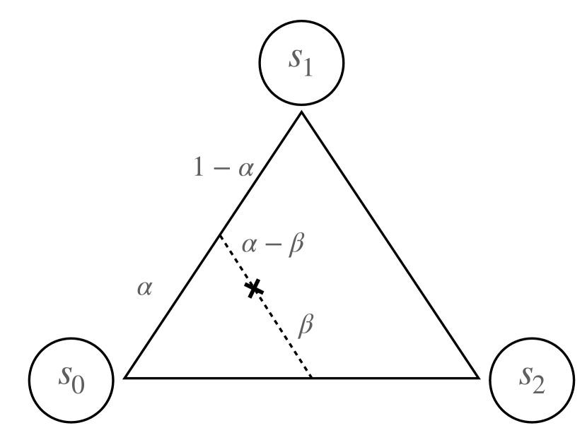
(a) The point $(1-\alpha,\beta,\alpha-\beta)$ in $\Delta(\{s_{0},s_{1},s_{2}\})$

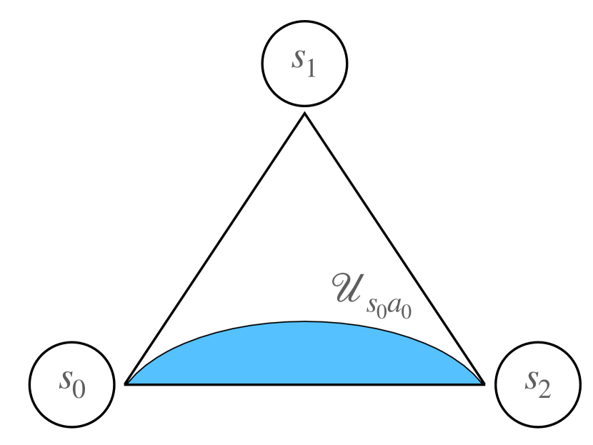
(b) The uncertainty set $\mathcal{U}_{s_{0}a_{0}}$ (in blue)

Figure 1: A simple robust MDP instance where $\inf_{\bm{P}\in\mathcal{U}}R_{{\sf avg}}(\pi,\bm{P})$ is not attained.

There are three states: $\mathcal{S}=\{s_{0},s_{1},s_{2}\}$, and only one action $a_{0}$, so that the RMDP reduces to the adversarial MDP with the adversary aiming at minimizing the average return. States $s_{1}$ and $s_{2}$ are absorbing states with reward $-1$ and $0$ respectively. The initial state is $s_{0}$, and the instantaneous reward in $s_{0}$ is $0$. Elements of $\Delta(\mathcal{S})$ are written $(p_{0},p_{1},p_{2})$, where $p_{i}$ is the probability of transitioning to state $s_{i}$. The uncertainty set is

$$\mathcal{U}_{s_{0}a_{0}}=\{\left(1-\alpha,\beta,\alpha-\beta\right)\in\Delta(\mathcal{S})\;|\;\alpha,\beta\in[0,1],\beta\leq\alpha(1-\alpha)\},$$

see Figure 1(a). Given $\left(1-\alpha,\beta,\alpha-\beta\right)\in\mathcal{U}_{s_{0}a_{0}}$, $\alpha$ is the probability to leave state $s_{0}$ and $\beta$ as the probability to go to state $s_{1}$.

The decision-maker has a single policy, which we denote $\pi=a_{0}$. We claim that $\inf_{\bm{P}\in\mathcal{U}_{s_{0}a_{0}}}R_{{\sf avg}}(\pi,\bm{P})=-1$, with $R_{{\sf avg}}(\pi,\bm{P})>-1$ for each $\bm{P}\in\mathcal{U}_{s_{0}a_{0}}$. We first compute the average return associated with a pair $(a_{0},\bm{P})$ with $\bm{P}\in\mathcal{U}_{s_{0}a_{0}}$, $\bm{P}=(1-\alpha,\beta,\alpha-\beta)$ with $\alpha,\beta\in[0,1]$. Given the instantaneous rewards in this instance, note that we always have $R_{{\sf avg}}(\pi,\bm{P})\in[-1,0]$. If $\alpha=0$, then the decision-maker never leaves $s_{0}$ and $R_{{\sf avg}}(\pi,\bm{P})=0.$ Otherwise, for every discount factor $\gamma\in(0,1)$, the discounted return $R_{\gamma}(a_{0},\bm{P})$ satisfies

$$(1-\gamma)R_{\gamma}(a_{0},\bm{P})=-\gamma\frac{\beta}{1-\gamma+\gamma\alpha}.$$

Therefore, taking the limit as $\gamma\rightarrow 1$, we obtain that if $\alpha>0$ we have $R_{{\sf avg}}(a_{0},\bm{P})=-\beta/\alpha$. Now consider $\alpha_{n}=1/n,\beta=\alpha_{n}(1-\alpha_{n}),\bm{P}_{n}=(1-\alpha_{n},\beta_{n},\alpha_{n}-\beta_{n})$ for $n\geq 1$. Then $R_{{\sf avg}}(a_{0},\bm{P}_{n})=-1+1/n\rightarrow-1$ as $n\rightarrow+\infty$. However, $-1$ is never attained by any stationary policy. Indeed, $R_{{\sf avg}}(a_{0},\bm{P})=-1\iff-\beta/\alpha=-1\iff\alpha=\beta$. But $\beta\leq\alpha(1-\alpha)$ by construction of $\mathcal{U}_{s_{0}a_{0}}$, so that $\beta=\alpha\Rightarrow\alpha=0$ for $\bm{P}\in\mathcal{U}_{s_{0}a_{0}}$. In this case, we have $R_{{\sf avg}}(,a_{0},\bm{P})=0$, which is a contradiction. ∎

Prior works on RMDPs have only focused on sa-rectangular RMDPs, either with polyhedral uncertainty set (Le Tallec, 2007; Tewari and Bartlett, 2007) or under the assumption that the Markov chains induced by any pair of policy and transition probabilities are unichain (Wang et al., 2023). In these special cases, we prove in Appendix 11 that $\inf_{\bm{P}\in\mathcal{U}}R_{{\sf avg}}(\pi,\bm{P})=\min_{\bm{P}\in\mathcal{U}}R_{{\sf avg}}(\pi,\bm{P})$, i.e., worst-case transition probabilities indeed exist for any stationary policy $\pi\in\Pi_{\sf S}$. We note that this question is not mentioned in prior work (Tewari and Bartlett, 2007; Wang et al., 2023).

We conclude this section with the following technical lemma. We adapt it from the literature on nominal MDP with a finite set of states and compact set of actions (Bierth, 1987). We briefly discuss this lemma in Appendix 12.

Lemma 3.3 (Adapted from theorem 2.5, Bierth (1987))

Let $\mathcal{U}$ be compact convex and s-rectangular. Let $\pi\in\Pi_{\sf S}$. Then

$$\inf_{\bm{P}\in\mathcal{U}_{\sf H}}R_{{\sf avg}}(\pi,\bm{P})=\inf_{\bm{P}\in\mathcal{U}}R_{{\sf avg}}(\pi,\bm{P}).$$

3.2 The case of sa-rectangular robust MDPs

We now focus on the case of sa-rectangular RMDPs. Our main result in this section is to show that there always exist average optimal policies that are stationary and deterministic, an attractive feature for practical implementation in real-world applications. In particular, we have the following theorem.

Theorem 3.4

Consider a sa-rectangular robust MDP with a compact convex uncertainty set $\mathcal{U}$. There exists an average optimal policy that is stationary and deterministic:

$$\sup_{\pi\in\Pi_{\sf H}}\inf_{\bm{P}\in\mathcal{U}}R_{{\sf avg}}(\pi,\bm{P})\;=\;\max_{\pi\in\Pi_{\sf SD}}\inf_{\bm{P}\in\mathcal{U}}R_{{\sf avg}}(\pi,\bm{P}).$$

The proof proceeds in two steps and leverages existing results from the literature on perfect information SGs (Gimbert and Kelmendi, 2023).

Proof.

Proof of Theorem 3.4. In the first step of the proof, we show that Theorem 3.4 is true in the special case where $\mathcal{U}$ is polyhedral. In this case, $\mathcal{U}$ only has a finite number of extreme points, and the robust MDP problem is equivalent to a perfect information stochastic game with finitely many actions for both players, as described in Section 2. We can then rely on the following crucial equality, which is a reformulation of proposition 3.2 in Gimbert and Kelmendi (2023):

$$\sup_{\pi\in\Pi_{\sf H}}\inf_{\bm{P}\in\mathcal{U}_{\sf H}}R_{{\sf avg}}(\pi,\bm{P})=\max_{\pi\in\Pi_{\sf SD}}\inf_{\bm{P}\in\mathcal{U}_{\sf H}}R_{{\sf avg}}(\pi,\bm{P})=\inf_{\bm{P}\in\mathcal{U}}\sup_{\pi\in\Pi_{\sf H}}R_{{\sf avg}}(\pi,\bm{P}).$$ (3.3)

From weak duality we always have $\sup_{\pi\in\Pi_{\sf H}}\inf_{\bm{P}\in\mathcal{U}}R_{{\sf avg}}(\pi,\bm{P})\leq\inf_{\bm{P}\in\mathcal{U}}\sup_{\pi\in\Pi_{\sf H}}R_{{\sf avg}}(\pi,\bm{P})$, and

$$\inf_{\bm{P}\in\mathcal{U}}\sup_{\pi\in\Pi_{\sf H}}R_{{\sf avg}}(\pi,\bm{P})=\max_{\pi\in\Pi_{\sf SD}}\inf_{\bm{P}\in\mathcal{U}_{\sf H}}R_{{\sf avg}}(\pi,\bm{P})\leq\max_{\pi\in\Pi_{\sf SD}}\inf_{\bm{P}\in\mathcal{U}}R_{{\sf avg}}(\pi,\bm{P})\leq\sup_{\pi\in\Pi_{\sf H}}\inf_{\bm{P}\in\mathcal{U}}R_{{\sf avg}}(\pi,\bm{P})$$

where the equality follows from (3.3), the second inequality follows from $\mathcal{U}\subset\mathcal{U}_{\sf H}$, and the last inequality follows from $\Pi_{\sf SD}\subset\Pi_{\sf H}$. Therefore, all terms above are equal, and we have

$$\sup_{\pi\in\Pi_{\sf H}}\inf_{\bm{P}\in\mathcal{U}}R_{{\sf avg}}(\pi,\bm{P})=\max_{\pi\in\Pi_{\sf SD}}\inf_{\bm{P}\in\mathcal{U}}R_{{\sf avg}}(\pi,\bm{P}).$$

In the second step of the proof, we show that Theorem 3.4 holds for general compact uncertainty sets, without the assumption that $\mathcal{U}$ is polyhedral as in the first step of the proof. Let $\epsilon>0.$ For each $\pi\in\Pi_{\sf SD}$, consider $\bm{P}^{\pi,\epsilon}\in\mathcal{U}$ such that

$$\inf_{\bm{P}\in\mathcal{U}}R_{{\sf avg}}(\pi,\bm{P})\leq R_{{\sf avg}}(\pi,\bm{P}^{\pi,\epsilon})\leq\inf_{\bm{P}\in\mathcal{U}}R_{{\sf avg}}(\pi,\bm{P})+\epsilon.$$

Note that $\bm{P}^{\pi,\epsilon}$ always exists by definition of the infimum and note that $\{\bm{P}^{\pi,\epsilon}\;|\;\pi\in\Pi_{\sf SD}\}$ is a finite set since $\Pi_{\sf SD}$ is a finite set. Let us now consider the sa-rectangular uncertainty set $\mathcal{U}_{\sf f}$ defined as the convex hull of the finite set $\{\bm{P}\;|\;\forall\;(s,a)\in\mathcal{S}\times\mathcal{A},\exists\pi\in\Pi_{\sf SD},\bm{p}_{sa}=\bm{p}_{sa}^{\pi}\}.$ By construction, $\mathcal{U}_{\sf f}$ is polyhedral and sa-rectangular. Additionally, $\mathcal{U}_{\sf f}\subset\mathcal{U}$, and for any $\pi\in\Pi_{\sf SD}$, we have

$$\inf_{\bm{P}\in\mathcal{U}}R_{{\sf avg}}(\pi,\bm{P})\leq\inf_{\bm{P}\in\mathcal{U}_{\sf f}}R_{{\sf avg}}(\pi,\bm{P})\leq\inf_{\bm{P}\in\mathcal{U}}R_{{\sf avg}}(\pi,\bm{P})+\epsilon.$$

Therefore,

$$\sup_{\pi\in\Pi_{\sf H}}\inf_{\bm{P}\in\mathcal{U}}R_{{\sf avg}}(\pi,\bm{P}) \leq\sup_{\pi\in\Pi_{\sf H}}\inf_{\bm{P}\in\mathcal{U}_{\sf f}}R_{{\sf avg}}(\pi,\bm{P})$$

$$=\max_{\pi\in\Pi_{\sf SD}}\inf_{\bm{P}\in\mathcal{U}_{\sf f}}R_{{\sf avg}}(\pi,\bm{P})$$

$$\leq\max_{\pi\in\Pi_{\sf SD}}\inf_{\bm{P}\in\mathcal{U}}R_{{\sf avg}}(\pi,\bm{P})+\epsilon.$$

where the first inequality uses $\mathcal{U}_{\sf f}\subset\mathcal{U}$, the equality follows from the first step of the proof and $\mathcal{U}_{\sf f}$ being polyhedral, and the last equality holds by construction of $\mathcal{U}_{\sf f}$. Therefore, for all $\epsilon>0$, we have $\sup_{\pi\in\Pi_{\sf H}}\inf_{\bm{P}\in\mathcal{U}}R_{{\sf avg}}(\pi,\bm{P})\leq\max_{\pi\in\Pi_{\sf SD}}\inf_{\bm{P}\in\mathcal{U}}R_{{\sf avg}}(\pi,\bm{P})+\epsilon$, and we can conclude that

$$\sup_{\pi\in\Pi_{\sf H}}\inf_{\bm{P}\in\mathcal{U}}R_{{\sf avg}}(\pi,\bm{P})\leq\max_{\pi\in\Pi_{\sf SD}}\inf_{\bm{P}\in\mathcal{U}}R_{{\sf avg}}(\pi,\bm{P})$$

which directly implies

$$\sup_{\pi\in\Pi_{\sf H}}\inf_{\bm{P}\in\mathcal{U}}R_{{\sf avg}}(\pi,\bm{P})=\max_{\pi\in\Pi_{\sf SD}}\inf_{\bm{P}\in\mathcal{U}}R_{{\sf avg}}(\pi,\bm{P}).$$

∎

Theorem 3.4 has several important consequences.

Closing an important gap in prior works. First, to the best of our knowledge, we are the first to study average return RMDPs in all generality without constraining the problem to stationary policies and to show that average optimal policies for sa-rectangular RMDPs may be chosen stationary and deterministic. Therefore, Theorem 3.4 addresses an important gap that has been entirely overlooked in the existing literature on RMDPs with average return (Tewari and Bartlett, 2007; Wang et al., 2023).

Strong duality and history-dependent adversary. Another consequence of Theorem 3.4 is the following strong duality theorem. We provide the detailed proof in Appendix 13.

Theorem 3.5

Consider a sa-rectangular robust MDP with a compact convex uncertainty set $\mathcal{U}$. Then the following strong duality results hold:

$$\sup_{\pi\in\Pi_{\sf H}}\inf_{\bm{P}\in\mathcal{U}}R_{{\sf avg}}(\pi,\bm{P}) =\inf_{\bm{P}\in\mathcal{U}}\sup_{\pi\in\Pi_{\sf H}}R_{{\sf avg}}(\pi,\bm{P})$$ (3.4)

$$\max_{\pi\in\Pi_{\sf SD}}\inf_{\bm{P}\in\mathcal{U}}R_{{\sf avg}}(\pi,\bm{P}) =\inf_{\bm{P}\in\mathcal{U}}\max_{\pi\in\Pi_{\sf SD}}R_{{\sf avg}}(\pi,\bm{P})$$ (3.5)

Theorem 3.5 is akin to the strong duality results for discounted RMDPs (Wiesemann et al., 2013; Goyal and Grand-Clément, 2022). It is interesting to note that strong duality still holds for sa-rectangular RMDPs with average optimality, especially as in Equality (3.5), since the maximum over $\pi\in\Pi_{\sf SD}$ is always attained (it is the maximum over a finite set) while the infimum over $\mathcal{U}$ may not be attained, even in very simple settings, as we illustrate in Proposition 3.2. Strong duality is crucial to study the case of history-dependent adversaries, as we now show. The case of non-stationary adversary has also gathered interest and is discussed in Iyengar (2005); Nilim and Ghaoui (2005). Interestingly, we show that this model is equivalent to (3.9), i.e., to the case of stationary adversaries in the following theorem. The proof is relatively concise and relies on our fundamental results from Theorem 3.4, Theorem 3.5 and on the properties of MDPs with compact action sets. We also note that it is straightforward to prove that the same results hold for Markovian adversaries.

Theorem 3.6

Consider a sa-rectangular robust MDP with a compact convex uncertainty set $\mathcal{U}$. Then

$$\sup_{\pi\in\Pi_{\sf H}}\inf_{\bm{P}\in\mathcal{U}_{\sf H}}R_{{\sf avg}}(\pi,\bm{P})\;=\;\sup_{\pi\in\Pi_{\sf H}}\inf_{\bm{P}\in\mathcal{U}}R_{{\sf avg}}(\pi,\bm{P}).$$

Proof.

Proof. We have

$$\inf_{\bm{P}\in\mathcal{U}_{\sf H}}\sup_{\pi\in\Pi_{\sf H}}R_{{\sf avg}}(\pi,\bm{P}) \leq\inf_{\bm{P}\in\mathcal{U}}\sup_{\pi\in\Pi_{\sf H}}R_{{\sf avg}}(\pi,\bm{P})$$

$$=\sup_{\pi\in\Pi_{\sf H}}\inf_{\bm{P}\in\mathcal{U}}R_{{\sf avg}}(\pi,\bm{P})$$

$$=\max_{\pi\in\Pi_{\sf SD}}\inf_{\bm{P}\in\mathcal{U}}R_{{\sf avg}}(\pi,\bm{P})$$

$$=\max_{\pi\in\Pi_{\sf SD}}\inf_{\bm{P}\in\mathcal{U}_{\sf H}}R_{{\sf avg}}(\pi,\bm{P})$$

$$\leq\sup_{\pi\in\Pi_{\sf H}}\inf_{\bm{P}\in\mathcal{U}_{\sf H}}R_{{\sf avg}}(\pi,\bm{P})$$

where the first inequality uses $\mathcal{U}\subset\mathcal{U}_{\sf H}$, where the first equality uses Theorem 3.5, the second equality uses Theorem 3.4, the third equality is from Lemma 3.3, and the last equality uses $\Pi_{\sf SD}\subset\Pi_{\sf H}$. ∎

Other natural definitions of average optimality. Other possible definitions of the average return criterion exist, such as, for $(\pi,\bm{P})\in\Pi_{\sf H}\times\mathcal{U}$, the following natural definitions:

$$\liminf_{T\rightarrow+\infty}\mathbb{E}_{\pi,\bm{P}}\left[\frac{1}{T+1}\sum_{t=0}^{T}r_{s_{t}a_{t}s_{t+1}}\;|\;s_{0}\sim\bm{p}_{0}\right],$$ (3.6)

$$\limsup_{T\rightarrow+\infty}\mathbb{E}_{\pi,\bm{P}}\left[\frac{1}{T+1}\sum_{t=0}^{T}r_{s_{t}a_{t}s_{t+1}}\;|\;s_{0}\sim\bm{p}_{0}\right],$$ (3.7)

$$\mathbb{E}_{\pi,\bm{P}}\left[\liminf_{T\rightarrow+\infty}\frac{1}{T+1}\sum_{t=0}^{T}r_{s_{t}a_{t}s_{t+1}}\;|\;s_{0}\sim\bm{p}_{0}\right].$$ (3.8)

Note that when $(\pi,\bm{P})\in\Pi_{\sf S}\times\mathcal{U}$, the three quantities in the above equations are equal to $R_{{\sf avg}}$ and are equal to

$$\lim_{T\rightarrow+\infty}\;\mathbb{E}_{\pi,\bm{P}}\left[\frac{1}{T+1}\sum_{t=0}^{T}r_{s_{t}a_{t}s_{t+1}}\;|\;s_{0}\sim\bm{p}_{0}\right]$$ (3.9)

but in all generality, we have following inequality (see lemma 2.1 in Feinberg and Shwartz (2012)):

$$\eqref{eq:exp-liminf}\leq~{}\eqref{eq:liminf-exp}\leq~{}\eqref{eq:limsup-exp}\leq R_{{\sf avg}}(\pi,\bm{P}),\forall\;(\pi,\bm{P})\in\Pi_{\sf H}\times\mathcal{U}.$$ (3.10)

At this point, the reader may wonder if the results that we proved in this section also hold for these other definitions of the average return and if these returns each need to be analyzed separately. Fortunately, based on Inequality (3.10), we can show in a straightforward manner that Theorem 3.4, Theorem 3.5 and Theorem 3.6 still hold for the average return as in $\eqref{eq:exp-liminf},\eqref{eq:liminf-exp}$ and $\eqref{eq:limsup-exp}$. This shows that all these definitions of the average return are equivalent in the sense that there exists a stationary deterministic policy that is average optimal simultaneously for all these objective functions. In particular, we obtain the following important corollary. For the sake of conciseness we provide the proof in Appendix 14.

Corollary 3.7

Consider a sa-rectangular robust MDP with a compact convex uncertainty set $\mathcal{U}$. Let $\hat{R}_{{\sf avg}}$ as defined in (3.6), (3.7), or (3.8).

1. There exists an average optimal policy that is stationary and deterministic, and which coincides with an average optimal policy for $R_{{\sf avg}}$ as in (3.1):

   $$\sup_{\pi\in\Pi_{\sf H}}\inf_{\bm{P}\in\mathcal{U}}\hat{R}_{{\sf avg}}(\pi,\bm{P})\;=\;\max_{\pi\in\Pi_{\sf SD}}\inf_{\bm{P}\in\mathcal{U}}\hat{R}_{{\sf avg}}(\pi,\bm{P})=\max_{\pi\in\Pi_{\sf SD}}\inf_{\bm{P}\in\mathcal{U}}R_{{\sf avg}}(\pi,\bm{P}).$$

2. The strong duality results from Theorem 3.5 still hold if we replace $R_{{\sf avg}}$ by $\hat{R}_{{\sf avg}}$.

3. The equivalence between stationary adversaries and history-dependent adversaries from Theorem 3.6 still hold if we replace $R_{{\sf avg}}$ by $\hat{R}_{{\sf avg}}$.

3.3 The case of s-rectangular robust MDPs

We now show that for s-rectangular RMDPs, Markovian policies may strictly outperform stationary policies for the average return criterion. This is a surprising result since stationary policies are sufficient for solving average sa-rectangular RMDPs and discount s-rectangular RMDPs. We rely on a stochastic game instance called The Big Match (Blackwell and Ferguson, 1968). In this instance, there are two absorbing states $A_{0}$ (with a reward of $0$) and $A_{1}$ (with a reward of $1$) and two non-absorbing state $s_{0}$ and $s_{1}$. The decision-maker starts in state $s_{0}$ and chooses an action in $\{T,B\}$. The adversary chooses the scalar $p\in[0,1]$, whose impact on the transitions is represented in Figure 2. Each arrow corresponds to a possible transition, and is labelled with its probability, and with the payoff obtained along this transition. If action $T$ is chosen, the game reaches an absorbing state, $A_{0}$ or $A_{1}$, depending on the choice of the adversary. If action $B$ is chosen, the decision-maker obtains a reward of $0$ or $1$ and the game continues. We can think of this instance as a game where the adversary tries to “guess” if the decision-maker will choose to stop the game (action $T$). If the adversary guesses correctly and the decision-maker chooses action $T$, the adversary can choose $p=1$ so that the decision-maker reaches the “bad” absorbing state $A_{0}$ (with reward $0$). Otherwise, if the decision-maker chooses action $B$, the game continues. The Big Match is represented in Figure 2. We will show that in The Big Match, all stationary policies have a worst-case average return of $0$, while a Markovian policy can achieve a worst-case average return of $1/2$. In particular, we have the following proposition.

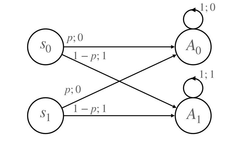
(a) Transition for action $T$

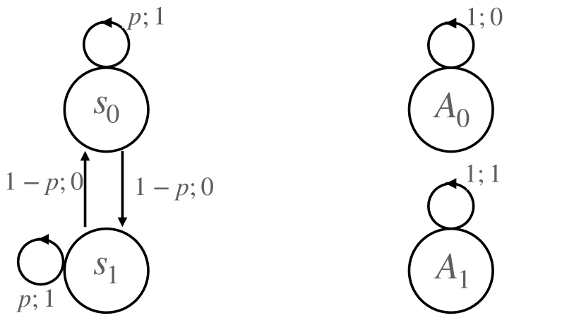
(b) Transition for action $B$

Figure 2: Transitions and rewards for The Big Match (Blackwell and Ferguson, 1968; Gillette, 1957) reformulated as an s-rectangular RMDP. The adversary chooses $p\in[0,1]$ and the decision-maker chooses an action in $\{T,B\}$.

Proposition 3.8

Consider the robust MDP instance from Figure 2 (The Big Match).

1. For any history-dependent policy $\pi\in\Pi_{\sf H}$, we have $\inf_{\bm{P}\in\mathcal{U}}R_{{\sf avg}}(\pi,\bm{P})\leq 1/2$.

2. There exists a Markovian policy $\pi\in\Pi_{\sf M}$ such that $\min_{\bm{P}\in\mathcal{U}}R_{{\sf avg}}(\pi,\bm{P})=1/2$.

3. For any stationary policy $\pi\in\Pi_{\sf S}$, we have $\min_{\bm{P}\in\mathcal{U}}R_{{\sf avg}}(\pi,\bm{P})=0$. Additionally, $\min_{\bm{P}\in\mathcal{U}}\max_{\pi\in\Pi_{\sf S}}R_{{\sf avg}}(\pi,\bm{P})=1/2$. Therefore, there is a duality gap in the case where the decision-maker is constrained to choose a stationary policy:

   $$\max_{\pi\in\Pi_{\sf S}}\min_{\bm{P}\in\mathcal{U}}R_{{\sf avg}}(\pi,\bm{P})=0<\min_{\bm{P}\in\mathcal{U}}\max_{\pi\in\Pi_{\sf S}}R_{{\sf avg}}(\pi,\bm{P})=1/2.$$

Proof.

Proof. We note that point 1 and point 3 are known in the SG literature, and only point 2 is new here. In particular, point 1 follows from Blackwell’s original argument, see the beginning of theorem 1 in Blackwell and Ferguson (1968), and point 3 is exactly Lemma 1, chapter 12, Neyman et al. (2003). We detail the proofs here for conciseness.

1. This follows from the adversary choosing the transition probabilities $\bm{P}$ corresponding to $p=1/2$. In this case, we have $R_{{\sf avg}}(\pi,\bm{P})=1/2$ for any policy $\pi\in\Pi_{\sf H}$. Indeed, if $\pi$ always selects action $B$, then clearly $R_{{\sf avg}}(\pi,\bm{P})=1/2$. Otherwise, there exists a period at which $\pi$ selects action $T$ with a positive probability, and in this case we also have $R_{{\sf avg}}(\pi,\bm{P})=1/2$ since the decision-maker is equally likely to reach the terminal state $A_{0}$ (with a reward of $0$) or the terminal state $A_{1}$ (with a reward of $1$).

2. We will construct a Markovian policy $\pi$ such that $R_{{\sf avg}}(\pi,\bm{P})=1/2$ for any $\bm{P}\in\mathcal{U}$. In particular, let $\pi$ the Markovian policy that chooses the same action in the states $s_{0}$ and $s_{1}$ and such that: (a) at time $t=0$, $\pi$ chooses action $T$ or action $B$ with probability $1/2$; (b) for any time $t\geq 1$, $\pi$ always chooses action $B$. Let $p\in[0,1]$ and let $\bm{P}\in\mathcal{U}$ be the corresponding transition probabilities. At time $t=0$, the game stops with probability $1/2$ (if action $T$ is chosen), in which case the decision-maker reaches $A_{0}$ with probability $p$, obtaining a reward of $0$ forever, and reaches $A_{1}$ with probability $1-p$, obtaining a reward of $1$ forever. If action $B$ is selected at time $t=0$, which happens with probability $1/2$, the game starts in $s_{0}$ or $s_{1}$ at time $t=1$. Then, action $B$ is selected forever, so that the average payoff is $(1-p).$ Overall, we obtain that the average payoff of $\pi$ is $\frac{1}{2}\times p+\frac{1}{2}\times(1-p)=\frac{1}{2}$.

3. Let $\pi\in\Pi_{\sf S}$. If $\pi$ always chooses action $B$, then the adversary choosing $p=0$ yields an average return of $0$. Otherwise, $\pi$ chooses action $T$ with a positive probability, and the adversary choosing $p=1$ yields an average return of $0$. Therefore, $\min_{\bm{P}\in\mathcal{U}}R_{{\sf avg}}(\pi,\bm{P})=0$ for any $\pi\in\Pi_{\sf S}$. The fact that $\min_{\bm{P}\in\mathcal{U}}\max_{\pi\in\Pi_{\sf S}}R_{{\sf avg}}(\pi,\bm{P})=1/2$ follows from point 1 in this proof: when $p=1/2$, we have $R_{{\sf avg}}(\pi,\bm{P})=1/2,\forall\;\pi\in\Pi_{\sf H}$.

∎

Proposition 3.8 shows the stark contrast between average optimal policies for sa-rectangular RMDPs, which can always be chosen stationary and deterministic (Theorem 3.4), and average optimal policies for s-rectangular RMDPs, which may have to be Markovian and randomized. Additionally, the last point of Proposition 3.8 shows that strong duality does not hold for average return s-rectangular RMDPs with stationary strategies for the decision-maker, again in contrast to the case of sa-rectangular RMDPs (Theorem 3.5). It is an interesting open question to understand if, for any s-rectangular RMDP, an average optimal policy may be chosen Markovian and if strong duality holds in the case of Markovian decisions for the decision-maker. We conclude this section with a comparison of The Big Match in the case of a history-dependent adversary. In this case, The Big Match is exactly the instance studied in the stochastic game literature. In particular, Blackwell and Ferguson (1968) show that in the classical SG setting where both the decision-maker and the adversary can use history-dependent policies, we have

$$\sup_{\pi\in\Pi_{\sf H}}\inf_{\bm{P}\in\mathcal{U}_{\sf H}}R_{{\sf avg}}(\pi,\bm{P})=\inf_{\bm{P}\in\mathcal{U}_{\sf H}}\sup_{\pi\in\Pi_{\sf H}}R_{{\sf avg}}(\pi,\bm{P})=1/2,$$

the supremum is not attained in the left-hand side above, any Markovian policy achieves a worst-case average return of $0$: $\inf_{\bm{P}\in\mathcal{U}_{\sf H}}R_{{\sf avg}}(\pi,\bm{P})=0$ for $\pi\in\Pi_{\sf M}$, and for any choice of $\epsilon\in(0,1/2)$, only history-dependent policies can guarantee a worst-case average reward of $1/2-\epsilon$. We refer to chapter 12 in Neyman et al. (2003) for a modern exposition of these results.

4 Robust MDPs with Blackwell optimality

We now study Blackwell optimality for rectangular RMDPs. As detailed in the introduction, Blackwell optimality provides an adequate optimality criterion when there is no natural notion of discounting. We first introduce (approximate) Blackwell optimality in Section 4.1. We then focus on sa-rectangular RMDPs in Section 4.2 and on s-rectangular RMDPs in Section 4.3.

4.1 Blackwell optimality and approximate Blackwell optimality

An important limitation of the average return is that it ignores any rewards obtained in finite time, which may be problematic. For instance, when optimizing patient trajectories over time, practitioners are concerned with long-term goals (typically, survival at discharge) but also with the current patient condition at any point in time. Blackwell optimality is a criterion that balances both long-term and short-term goals by accounting for an entire range of discount factors. In particular, a policy is Blackwell optimal if it is discount optimal for all discount factors sufficiently close to $1$ (Puterman, 2014).

Definition 4.1

Let $\mathcal{U}$ be s-rectangular and convex compact. A policy $\pi\in\Pi_{\sf H}$ is Blackwell optimal if there exists $\gamma_{0}\in(0,1)$ such that

$$\min_{\bm{P}\in\mathcal{U}}R_{\gamma}(\pi,\bm{P})\geq\sup_{\pi\in\Pi_{\sf S}}\min_{\bm{P}\in\mathcal{U}}R_{\gamma}(\pi^{\prime},\bm{P}),\quad\forall\;\gamma\in(\gamma_{0},1).$$ (4.1)

For nominal MDPs, i.e. for the case where $\mathcal{U}$ is a singleton and the sets $\mathcal{S},\mathcal{A}$ are finite, there always exists a Blackwell optimal policy (Puterman, 2014). We will be interested in the existence (or not) of Blackwell optimal policies for rectangular robust MDPs. We also introduce the following definition of approximate Blackwell optimality, where a policy remains $\epsilon$-optimal for all discount factors sufficiently large.

Definition 4.2 ($\epsilon$-Blackwell optimality.)

Let $\mathcal{U}$ be s-rectangular and convex compact. A policy $\pi\in\Pi_{\sf H}$ is $\epsilon$-Blackwell optimal for $\epsilon>0$ if there exists a discount factor $\gamma_{\epsilon}\in(0,1)$ such that

$$\min_{\bm{P}\in\mathcal{U}}\,(1-\gamma)R_{\gamma}(\pi,\bm{P})\;\geq\;\sup_{\pi\in\Pi_{\sf S}}\min_{\bm{P}\in\mathcal{U}}\,(1-\gamma)R_{\gamma}(\pi^{\prime},\bm{P})-\epsilon,\quad\forall\;\gamma\in(\gamma_{\epsilon},1).$$ (4.2)

Note that we renormalize the discounted returns in the robust MDPs with the multiplicative term $(1-\gamma)$ since they may be unbounded otherwise. To the best of our knowledge, we are the first to introduce and study the notion of $\epsilon$-Blackwell optimality for robust MDPs. In the rest of this section, we will repeatedly use the following result pertaining to the existence of approximate Blackwell optimal policy in the adversarial MDP, which we adapt from the literature on MDPs with compact action sets.

Theorem 4.3 (Corollary 5.26, Sorin (2002))

Let $\mathcal{U}$ be a compact convex s-rectangular uncertainty set. Let $\pi\in\Pi_{\sf S}$ and $\epsilon>0$. Then there exist $\gamma_{\epsilon}\in(0,1)$ and $\bm{P}_{\epsilon}\in\mathcal{U}$ such that

$$\min_{\bm{P}\in\mathcal{U}}(1-\gamma)R_{\gamma}(\pi,\bm{P})\leq(1-\gamma)R_{\gamma}(\pi,\bm{P}_{\epsilon})\leq\min_{\bm{P}\in\mathcal{U}}(1-\gamma)R_{\gamma}(\pi,\bm{P})+\epsilon,\forall\;\gamma\in(\gamma_{\epsilon},1).$$

4.2 The case of sa-rectangular robust MDPs

In this section, we provide a complete analysis of Blackwell optimality for sa-rectangular RMDPs. In Section 4.2.1, we first show that, surprisingly, a Blackwell optimal policy may not exist, although an approximate Blackwell optimal policy may always be chosen stationary and deterministic. Additionally, this approximate Blackwell optimal policy is average optimal, as we show in Section 4.2.2. Finally, in Section 4.2.3 we introduce the notion of definable uncertainty sets, a very general class of uncertainty for which a Blackwell optimal policy exists.

4.2.1 Existence and non-existence results

We first contrast the existence properties of Blackwell optimal policies and $\epsilon$-Blackwell optimal policies (as introduced in Definition 4.2). Surprisingly, there are some examples of sa-rectangular robust MDPs where there are no Blackwell optimal policies, as stated formally in the next theorem.

Theorem 4.4

There exists a sa-rectangular robust MDP instance, with a compact convex uncertainty set $\mathcal{U}$, such that there is no Blackwell optimal policy:

$$\forall\;\pi\in\Pi_{\sf H},\forall\;\gamma\in(0,1),\exists\;\gamma^{\prime}\in(\gamma,1),\min_{\bm{P}\in\mathcal{U}}R_{\gamma^{\prime}}(\pi,\bm{P})<\sup_{\pi^{\prime}\in\Pi_{\sf S}}\min_{\bm{P}\in\mathcal{U}}R_{\gamma^{\prime}}(\pi^{\prime},\bm{P}).$$

To the best of our knowledge, we are the first to show that Blackwell optimal policies may not exist for sa-rectangular RMDPs. Indeed, Theorem 4.4 is surprising because the existence of Blackwell optimal policies has been proved in various other related frameworks, including nominal MDPs (Puterman, 2014), or sa-rectangular RMDPs under some additional assumptions (Goyal and Grand-Clément, 2022; Wang et al., 2023). For the sake of conciseness, we defer the proof of Theorem 4.4 in Appendix 15, and we only provide here some intuition on the main reasons behind the potential non-existence of Blackwell optimal policies.

Our proof of Theorem 4.4 is based on the same simple counterexample as for Proposition 3.2. We consider the same instance but where there are two available actions $a_{1}$ and $a_{2}$ at the non-absorbing state $s_{0}$. We can identify stationary policies with actions $a_{1}$ and $a_{2}$. The main property of our counterexample is that the robust value functions $\gamma\mapsto v^{a_{1},\mathcal{U}}_{s_{0},\gamma}$ and $\gamma\mapsto v^{a_{2},\mathcal{U}}_{s_{0},\gamma}$ have an oscillatory behaviour when $\gamma$ approaches $1$. As these robust value functions oscillate more and more often as $\gamma\rightarrow 1$, they intersect infinitely often on any interval close to $1$, so that there are no discount factors close enough to $1$ after which $a_{1}$ (or $a_{2}$) always remains a discount optimal policy. To obtain the oscillatory behaviours of the robust value functions, we construct two convex compact uncertainty sets $\mathcal{U}_{s_{0}a_{1}}$ and $\mathcal{U}_{s_{0}a_{2}}$. At a high level, we construct these uncertainty sets so that their boundaries overlap and intersect infinitely often, while remaining distinct sets (as subsets of $\Delta(\mathcal{S})$). Let us define the worst-case transition probabilities $\gamma\mapsto\bm{P}^{a_{1},\star}_{\gamma}$ and $\gamma\mapsto\bm{P}^{a_{2},\star}_{\gamma}$ for actions $a_{1}$ and $a_{2}$. Then these worst-case transition probabilities vary with $\gamma$ and always belong to the boundaries of $\mathcal{U}_{s_{0}a_{1}}$ and $\mathcal{U}_{s_{0}a_{2}}$. The infinite intersections of these boundaries induce a pathological, oscillating behaviour of $\gamma\mapsto v^{a_{1},\mathcal{U}}_{s_{0},\gamma}=v^{a_{1},\bm{P}^{a_{1},\star}_{\gamma}}_{s_{0},\gamma}$ (and similarly for $a_{2}$). Our analysis also explains why this pathological behaviour is impossible in nominal MDPs: the transition probabilities is fixed, and in this case $\gamma\mapsto v^{\pi,\bm{P}}_{s,\gamma}$ is always a well-behaved (rational) function. This pathological behaviour is also impossible for polyhedral uncertainty: the worst-case transition probabilities remain the same for $\gamma$ large enough, as shown in (Goyal and Grand-Clément, 2022).

Since Theorem 4.4 shows that Blackwell optimal policies may not always exist, it is natural to ask if approximate Blackwell optimal policies always exist. We answer this question by the positive in the next theorem. In fact, we show the following stronger existence result.

Theorem 4.5

Let $\mathcal{U}$ be a sa-rectangular compact uncertainty set. Then there exists a stationary deterministic policy that is $\epsilon$-Blackwell optimal for all $\epsilon>0$, i.e., $\exists\;\pi\in\Pi_{\sf SD},\forall\;\epsilon>0,\exists\;\gamma_{\epsilon}\in(0,1)$ such that

$$\min_{\bm{P}\in\mathcal{U}}(1-\gamma)R_{\gamma}(\pi,\bm{P})\geq\sup_{\pi^{\prime}\in\Pi_{\sf S}}\min_{\bm{P}\in\mathcal{U}}(1-\gamma)R_{\gamma}(\pi^{\prime},\bm{P})-\epsilon,\forall\;\gamma\in(\gamma_{\epsilon},1).$$

Theorem 4.5 shows another surprising result: not only there exists an $\epsilon$-Blackwell optimal policy for any choice of $\epsilon>0$, but in fact, we can choose the same stationary deterministic policy $\pi\in\Pi_{\sf SD}$ to be $\epsilon$-Blackwell optimal for all $\epsilon.$ Theorem 4.4 shows that we can not choose $\epsilon=0$ in the statement of Theorem 4.5. We present the proof in Appendix 16. The main idea is to exploit Theorem 4.3, i.e., the existence of approximate Blackwell optimal policies in the adversarial MDP.

4.2.2 Limit behaviours and connection with average optimality

We now highlight the connection between Blackwell optimality and average optimality. Intuitively, approximate Blackwell optimal policies remain $\epsilon$-optimal for all $\gamma$ close to $1$. Since the discount factor captures the willingness of the decision-maker to wait for future rewards, we expect that the discounted return resembles more and more the average return as $\gamma\rightarrow 1$. We show that this intuition is correct for sa-rectangular uncertainty sets in the following theorem.

Theorem 4.6

Consider a sa-rectangular robust MDP with a compact convex uncertainty set $\mathcal{U}$. Let $\pi\in\Pi_{\sf SD}$ be $\epsilon$-Blackwell optimal, for all $\epsilon>0$. Then $\pi$ is also average optimal.

The proof of Theorem 4.6 is presented in Appendix 17. The main lines of the proof are instructive and rely on carefully inspecting the limit behavior of the discounted return as $\gamma\rightarrow 1$. We provide an outline here. Recall that we always have

$$\lim_{\gamma\rightarrow 1}(1-\gamma)R_{\gamma}(\pi,\bm{P})=R_{{\sf avg}}(\pi,\bm{P}),\forall\;(\pi,\bm{P})\in\Pi_{\sf S}\times\mathcal{U}.$$

The first step is to show that the equality above is still true when taking the worst-case over the transition probabilities. In particular, we show the following lemma.

Lemma 4.7

In the setting of Theorem 4.6, let $\pi\in\Pi_{\sf S}.$ Then $\min_{\bm{P}\in\mathcal{U}}(1-\gamma)R_{\gamma}(\pi,\bm{P})$ admits a limit as $\gamma\rightarrow 1$ and

$$\lim_{\gamma\rightarrow 1}\min_{\bm{P}\in\mathcal{U}}(1-\gamma)R_{\gamma}(\pi,\bm{P})=\inf_{\bm{P}\in\mathcal{U}}R_{{\sf avg}}(\pi,\bm{P}).$$

We then show that the same conclusion holds for the limit of the optimal discounted return.

Lemma 4.8

In the setting of Theorem 4.6, $\max_{\pi\in\Pi_{\sf SD}}\min_{\bm{P}\in\mathcal{U}}(1-\gamma)R_{\gamma}(\pi,\bm{P})$ admits a limit as $\gamma\rightarrow 1$ and

$$\lim_{\gamma\rightarrow 1}\max_{\pi\in\Pi_{\sf SD}}\min_{\bm{P}\in\mathcal{U}}(1-\gamma)R_{\gamma}(\pi,\bm{P})=\max_{\pi\in\Pi_{\sf SD}}\inf_{\bm{P}\in\mathcal{U}}R_{{\sf avg}}(\pi,\bm{P}).$$

The last part of the proof relates average optimality and approximate-Blackwell optimality.

Lemma 4.9

In the setting of Theorem 4.6, let $\pi\in\Pi_{\sf SD}$ be $\epsilon$-Blackwell optimal for any $\epsilon>0$. Then

$$\lim_{\gamma\rightarrow 1}\min_{\bm{P}\in\mathcal{U}}(1-\gamma)R_{\gamma}(\pi,\bm{P})=\lim_{\gamma\rightarrow 1}\max_{\pi^{\prime}\in\Pi_{\sf SD}}\inf_{\bm{P}\in\mathcal{U}}(1-\gamma)R_{\gamma}(\pi^{\prime},\bm{P}).$$

Combining Lemma 4.9 with Lemma 4.8 concludes the proof of Theorem 4.6. Note that all the conclusions from Lemma 4.7, Lemma 4.8 and Lemma 4.9 are true when we replace $R_{{\sf avg}}$ as defined in (3.1) by the other natural definitions $\eqref{eq:liminf-exp},\eqref{eq:limsup-exp}$, or $\eqref{eq:exp-liminf}$, since the lemmas above only involve maximization and minimization over $\Pi_{\sf S}$ and $\mathcal{U}$, over which $R_{{\sf avg}}$ and the other definitions of the average return coincide.

Remark 4.10

Lemma 4.8 and Lemma 4.9 are present as corollary 4 in Tewari and Bartlett (2007), under the assumption that $\mathcal{U}$ is based on $\ell_{\infty}$-distance. This considerably simplifies the proof, as in this setting, the number of extreme points of $\mathcal{U}$ is finite, so the infimum over $\mathcal{U}$ can be reduced to a minimum over a finite number of elements, and we can exchange the minimization with the limit. Lemma 4.7 is also present in Wang et al. (2023), under some additional assumptions (unichain compact sa-rectangular RMDPs). Our results show that the unichain assumption is unnecessary.

4.2.3 Definable robust Markov decision processes

In this section, we introduce a very general class of uncertainty sets that encompasses virtually all the practical examples existing in the RMDP literature, and for which stationary deterministic Blackwell optimal policies exist. Indeed, it is classical to construct uncertainty sets based on simple functions, like affine maps, $\ell_{p}$-balls, or Kullback-Leibler divergence, see Section 2. For this kind of simple functions, intuitively we do not expect that the robust value functions oscillate and intersect infinitely often. Our main contribution in this section is to formalize this intuition with the notion of definability (Van Den Dries, 1998; Coste, 2000; Bolte et al., 2015) and to prove Theorem 4.20, which states that for definable sa-rectangular RMDPs there always exists a stationary deterministic Blackwell optimal policy.

A concise introduction to definability. We start with the following definition. Intuitively, a set is definable if it is simple enough to be “constructed” based on polynomials, the exponential function, and canonical projections (elimination of variables).

Definition 4.11 (Definable set and definable function)

A subset of $\mathbb{R}^{n}$ is definable if it is of the form

$$\{\bm{x}\in\mathbb{R}^{n}\;|\exists k\in\mathbb{N},\exists\bm{y}\in\mathbb{R}^{k},\;P\left(x_{1},...,x_{n},y_{1},...,y_{k},\exp(x_{1}),...,\exp(x_{n}),...,\exp(y_{1}),...,\exp(y_{k})\right)=0\}$$ (4.3)

where $P:\mathbb{R}^{2(n+k)}\rightarrow\mathbb{R}$ is a real polynomial. For $\Omega\subset\mathbb{R}^{n}$ a definable susbet of $\mathbb{R}^{n}$, a function $f:\Omega\rightarrow\mathbb{R}^{m}$ is definable if its graph $\{(\bm{x},\bm{y})\in\Omega\times\mathbb{R}^{m}\;|\;\bm{y}=f(\bm{x})\}$ is a definable set in $\mathbb{R}^{n+m}$.

We refer to Bolte et al. (2015) and Akian et al. (2019) for concise introductions to definability and to Coste (2000) for a more in-depth treatment. It is instructive to start by studying a few simple examples.

Example 4.12 (Affine functions.)

Consider an affine function $f:\bm{x}\mapsto\bm{a}^{\top}\bm{x}+b$ for some $\bm{a}\in\mathbb{R}^{\mathcal{S}},b\in\mathbb{R}$. The graph of $f$ is $\{(\bm{x},y)\in\mathbb{R}^{\mathcal{S}}\times\mathbb{R}\;|\;\sum_{s\in\mathcal{S}}a_{s}x_{s}+b-y=0\}$, which can be written as (4.3). Therefore, affine functions are definable.

Example 4.13 ($\ell_{p}$-norms.)

Consider an $\ell_{p}$-norm for $p\in\mathbb{N}$. Then its graph is $\{(\bm{x},y)\in\mathbb{R}^{\mathcal{S}}\times\mathbb{R}\;|\;\sum_{s\in\mathcal{S}}x_{s}^{p}-y^{p}=0\}$, which can be written as (4.3). Therefore, $\ell_{p}$-norms are definable.

Example 4.14 (Logarithm and exponential.)

It is straightforward that $x\mapsto\exp(x)$ is a definable function. The graph of the logarithm is $\{(x,y)\in\mathbb{R}_{+}^{*}\times\mathbb{R}\;|\;y=\log(x)\}$. This can be rewritten $\{(x,y)\in\mathbb{R}_{+}^{*}\times\mathbb{R}\;|\;\exp(y)=x\}$, which is a definable set. Therefore, the logarithm is a definable function.

Definable functions and definable sets are well-behaved under many useful operations, as shown in the following lemma. The proof follows directly from the definition and some properties shown in Bolte et al. (2015), and we present it for completeness in Appendix 18.

Lemma 4.15

1. If $A,B\subset\mathbb{R}^{n}$ are definable sets, then $A\cup B,A\cap B$ and $\mathbb{R}^{n}\setminus A$ are definable sets.

2. Let $f,g$ be definable functions. Then $f\circ g$, $-f$, $f+g$, $f\times g$ are definable.

3. For $A,B$ two definable sets and $g:A\times B\rightarrow\mathbb{R}$ a definable function, then $A\rightarrow\mathbb{R},\bm{x}\mapsto\inf_{\bm{y}\in B}g(\bm{x},\bm{y})$ and $A\rightarrow\mathbb{R},\bm{x}\mapsto\sup_{\bm{y}\in B}g(\bm{x},\bm{y})$ are definable functions.

4. If $A,B,g:A\rightarrow\mathbb{R}$ are definable then $g^{-1}(B)$ is definable.

Example 4.16 (Functions based on entropy.)

Let $\hat{\bm{p}}\in\Delta(\mathcal{A})$ with $\hat{p}_{s}>0,\forall\;s\in\mathcal{S}$. Consider the Kullback-Leibler divergence: $f:\bm{p}\mapsto\sum_{s\in\mathcal{S}}p_{s}\log(p_{s}/\hat{p}_{s})$ defined over $\bm{p}\in\Delta(\mathcal{S})$. Recall that $x\mapsto\log(x)$ is definable, so that $x\mapsto x\log(x)$ is also definable. By summation, the Kullback-Leibler divergence is a definable function. The case of the Burg entropy $\bm{p}\mapsto\sum_{s\in\mathcal{S}}\hat{p}_{s}\log(\hat{p}_{s}/p_{s})$ for $\bm{p}\in\Delta(\mathcal{S})$ is similar to the case of the Kullback-Leibler divergence.

The most important result for our use of definability is the following monotonicity theorem concerning definable functions of a real variable.

Theorem 4.17 (Theorem 2.1, Coste (2000))

Let $f:(a,b)\rightarrow\mathbb{R}$ be a definable function. Then there exists a finite subdivision of the interval $(a,b)$ as $a=a_{1}<a_{2}<\dots<a_{k}=b$ such that on each $(a_{i},a_{i+1})$ for $i=1,...,k-1$, $f$ is continuous and either constant or strictly monotone.

The monotonicity theorem shows that definable functions over $\mathbb{R}$ cannot oscillate infinitely often on an interval. Recall in the previous section, we have identified oscillations of the robust value functions as the main issue potentially precluding the existence of Blackwell optimal policies, see discussion after Theorem 4.4. Therefore, the monotonicity theorem will play an important role in our proof of the existence of Blackwell optimality for definable RMDPs as in Theorem 4.20.

Remark 4.18

The notion of definability is usually introduced in much more generality, e.g. (Van Den Dries, 1998; Coste, 2000; Bolte et al., 2015). We only introduce the notions necessary for this paper. For exactness, we simply note that in the literature, the notion of definability introduced in Definition 4.11 is usually referred to as definable in the real exponential field.

Definable robust MDPs. We now study sa-rectangular robust MDPs with a definable compact uncertainty set. We first note that this encompasses the vast majority of the uncertainty sets studied in the robust MDP literature. Indeed, from Lemma 4.15, we know that the set $\mathcal{U}_{sa}=\{\bm{p}\in\Delta(\mathcal{S})\;|\;d_{sa}\left(\bm{p}\right)\leq\alpha_{sa}\}$ is definable as soon as $d_{sa}:\mathbb{R}^{\mathcal{S}}\rightarrow\mathbb{R}$ is definable. From the various examples introduced above, we obtain that sa-rectangular uncertainty sets based on $\ell_{\infty}$-norm (Givan et al., 1997), $\ell_{2}$-norm (Iyengar, 2005), $\ell_{1}$-norm (Ho et al., 2021), Kullback-Leibler divergence and Burg entropy (Iyengar, 2005; Ho et al., 2022) are definable uncertainty sets.

We start by describing an appealing property of definable RMDPs: the robust value functions are themselves definable functions. In particular, we have the following proposition.

Proposition 4.19

Assume that $\mathcal{U}$ is sa-rectangular and definable. Then for any policy $\pi\in\Pi_{\sf S}$, the function $\gamma\mapsto\bm{v}^{\pi,\mathcal{U}}_{\gamma}$ is a definable function.

Proof.

Proof of Proposition 4.19. Recall that the robust value function $\bm{v}^{\pi,\mathcal{U}}_{\gamma}$ is the unique fixed-point of the following operator $\bm{v}\mapsto T^{\pi,\mathcal{U}}_{\gamma}(\bm{v})$, defined as

$$T^{\pi,\mathcal{U}}_{\gamma,s}(\bm{v})=\min_{\bm{P}_{s}\in\mathcal{U}_{s}}\sum_{a\in\mathcal{A}}\pi_{sa}\bm{p}_{sa}^{\top}\left(\bm{r}_{sa}+\gamma\bm{v}\right),\forall\;s\in\mathcal{S},\forall\;\bm{v}\in\mathbb{R}^{\mathcal{S}}.$$

The proof proceeds in two steps. The first step shows that $T^{\pi,\mathcal{U}}_{\gamma}$ is definable when $\mathcal{U}$ is definable. The second step shows that this is sufficient to conclude that the robust value functions are definable.

First step.

We first prove that $(\bm{v},\gamma)\mapsto T^{\pi,\mathcal{U}}_{\gamma}(\bm{v})$ is definable.

Note that a function is definable if and only if each of its components is definable (exercise 1.10, Coste (2000)). We want to show that $(\bm{v},\gamma)\mapsto\left(\sum_{a\in\mathcal{A}}\pi_{sa}\min_{\bm{p}_{sa}\in\mathcal{U}_{sa}}\bm{p}_{sa}^{\top}\left(\bm{r}_{sa}+\gamma\bm{v}\right)\right)_{s\in\mathcal{S}}$ is definable. Let $\bm{v}\in\mathbb{R}^{\mathcal{S}}$. The map $\gamma\mapsto\left(\sum_{a\in\mathcal{A}}\pi_{sa}\min_{\bm{p}_{sa}\in\mathcal{U}_{sa}}\bm{p}_{sa}^{\top}\left(\bm{r}_{sa}+\gamma\bm{v}\right)\right)_{s\in\mathcal{S}}$ is affine and therefore it is definable. We now fix $\gamma\in(0,1)$. From Lemma 4.15, if $\mathcal{U}_{sa}$ is definable for each pair $(s,a)\in\mathcal{S}\times\mathcal{A}$, then $\bm{v}\mapsto\min_{\bm{p}_{sa}\in\mathcal{U}_{sa}}\bm{p}_{sa}^{\top}\bm{v}$ is definable, and we conclude that $\bm{v}\mapsto\sum_{a\in\mathcal{A}}\pi_{sa}\min_{\bm{p}_{sa}\in\mathcal{U}_{sa}}\bm{p}_{sa}^{\top}\left(\bm{r}_{sa}+\gamma\bm{v}\right)$ is definable for any $s\in\mathcal{S}$. This shows that $\bm{v}\mapsto(\sum_{a\in\mathcal{A}}\pi_{sa}\min_{\bm{p}_{sa}\in\mathcal{U}_{sa}}\bm{p}_{sa}^{\top}\left(\bm{r}_{sa}+\gamma\bm{v}\right))_{s\in\mathcal{S}}$ is definable.

Second step.

We now show that $\gamma\mapsto\bm{v}^{\pi,\mathcal{U}}_{\gamma}$ is definable.

By definition, $\gamma\mapsto\bm{v}^{\pi,\mathcal{U}}_{\gamma}$ is definable if and only if its graph $\{\left(\bm{v},\gamma\right)\in\mathbb{R}^{\mathcal{S}}\times\mathbb{R}\;|\;\bm{v}=\bm{v}^{\pi,\mathcal{U}}_{\gamma}\}$ is definable. Note that $\{\left(\bm{v},\gamma\right)\in\mathbb{R}^{\mathcal{S}}\times\mathbb{R}\;|\;\bm{v}=\bm{v}^{\pi,\mathcal{U}}_{\gamma}\}=\{\left(\bm{v},\gamma\right)\in\mathbb{R}^{\mathcal{S}}\times\mathbb{R}\;|\;T^{\pi,\mathcal{U}}_{\gamma}(\bm{v})=\bm{v}\}$, since $\bm{v}^{\pi,\mathcal{U}}_{\gamma}$ is the unique fixed-point of the operator $T^{\pi,\mathcal{U}}_{\gamma}$. Since $\left(\bm{v},\gamma\right)\mapsto T^{\pi,\mathcal{U}}_{\gamma}(\bm{v})$ is definable, its graph $\{\left(\bm{v},\gamma,\bm{z}\right)\in\mathbb{R}^{\mathcal{S}}\times\mathbb{R}\times\mathbb{R}^{\mathcal{S}}\;|\;\bm{z}=T^{\pi,\mathcal{U}}_{\gamma}(\bm{v})\}$ is definable. Note that the set $\{\left(\bm{v},\gamma,\bm{z}\right)\mathbb{R}^{\mathcal{S}}\times\mathbb{R}\times\mathbb{R}^{\mathcal{S}}\;|\;\bm{z}=\bm{v}\}$ is also definable. Therefore their intersection is definable, i.e., the set $\{\left(\bm{v},\gamma,\bm{z}\right)\mathbb{R}^{\mathcal{S}}\times\mathbb{R}\times\mathbb{R}^{\mathcal{S}}\;|\;\bm{z}=T^{\pi,\mathcal{U}}_{\gamma}(\bm{v}),\bm{z}=\bm{v}\}$ is definable. This set can be rewritten $\{\left(\bm{v},\gamma,\bm{z}\right)\mathbb{R}^{\mathcal{S}}\times\mathbb{R}\times\mathbb{R}^{\mathcal{S}}\;|\;\bm{v}=T^{\pi,\mathcal{U}}_{\gamma}(\bm{v}),\bm{z}=\bm{v}\}$. Now if we project this set onto the components $\left(\bm{v},\gamma\right)\in\mathbb{R}^{\mathcal{S}}\times\mathbb{R}$, we obtain that the following set is definable: $\{\left(\bm{v},\gamma\right)\in\mathbb{R}^{\mathcal{S}}\times\mathbb{R}\;|\;\bm{v}=T^{\pi,\mathcal{U}}_{\gamma}(\bm{v})\}.$ This is precisely the graph of $\gamma\mapsto\bm{v}^{\pi,\mathcal{U}}_{\gamma}$, which concludes the proof. ∎Proposition 4.19 shows an appealing property of the robust value functions of definable robust MDPs: the robust value functions of stationary policies are definable functions. From the monotonicity theorem, two robust value functions can only intersect a finite number of times (or be equal on an entire interval close to $1$), which precludes the pathological behaviours underpinning the counterexample for the non-existence of Blackwell optimal policies (Theorem 4.4). We are now ready to state our main theorem for this section, which formalizes this intuition and shows that Blackwell optimal policies exist for the class of sa-rectangular definable RMDPs.

Theorem 4.20

Consider a sa-rectangular robust MDP with a definable compact convex uncertainty set $\mathcal{U}$. Then there exists a stationary deterministic Blackwell optimal policy:

$$\exists\;\pi\in\Pi_{\sf SD},\exists\;\gamma_{0}\in(0,1),\forall\;\gamma\in(\gamma_{0},1),\min_{\bm{P}\in\mathcal{U}}R_{\gamma}(\pi,\bm{P})\geq\sup_{\pi^{\prime}\in\Pi_{\sf S}}\min_{\bm{P}\in\mathcal{U}}R_{\gamma}(\pi^{\prime},\bm{P}).$$

Proof.

Proof of Theorem 4.20 From Proposition 4.19 and Lemma 4.15, we know that for each pair of stationary deterministic policies $\pi,\pi^{\prime}$ the function $[0,1)\rightarrow\mathbb{R},\gamma\mapsto v^{\pi,\mathcal{U}}_{\gamma,s}-v^{\pi^{\prime},\mathcal{U}}_{\gamma,s}$ is definable. From the monotonicity theorem, we can conclude that $\gamma\mapsto v^{\pi,\mathcal{U}}_{\gamma,s}-v^{\pi^{\prime},\mathcal{U}}_{\gamma,s}$ does not change signs in a neighborhood $(1-\eta(\pi,\pi^{\prime},s),1)$ with $\eta(\pi,\pi^{\prime},s)>0$. We then define $\bar{\gamma}=\max_{\pi,\pi^{\prime}\in\Pi_{\sf SD},s\in\mathcal{S}}1-\eta(\pi,\pi^{\prime},s)$ with $\bar{\gamma}<1$ since there are finitely many stationary deterministic policies and finitely many states. Any policy that is discount optimal for $\gamma\in(\bar{\gamma},1)$ is Blackwell optimal, which shows the existence of a stationary deterministic Blackwell optimal policy. ∎

The proof of Theorem 4.20 is relatively concise. It is also quite instructive, as it shows the existence of a Blackwell discount factor $\gamma_{\sf bw}\in(0,1)$, above which any discount optimal policy is also Blackwell optimal. We note that we actually proved a stronger result than the existence of a Blackwell optimal policy. In particular, we have shown the following theorem.

Theorem 4.21

Consider a sa-rectangular robust MDP with a definable compact convex uncertainty set $\mathcal{U}$. Then there exists a Blackwell discount factor $\gamma_{{\sf bw}}\in(0,1)$, such that any policy that is discount optimal for $\gamma\in(\gamma_{{\sf bw}},1)$ is also Blackwell optimal.

The existence of the Blackwell discount factor is shown in Grand-Clément and Petrik (2023) for nominal MDPs and for sa-rectangular RMDPs with polyhedral uncertainty sets. Theorem 4.21 extends this result to the larger class of definable uncertainty sets. If we know an upper bound $\hat{\gamma}<1$ on $\gamma_{{\sf bw}}$, then we can compute a Blackwell optimal policy by solving a discounted robust MDP with discount factor $\gamma=\hat{\gamma}$. We leave computing such an upper bound on $\gamma_{{\sf bw}}$ as an interesting future direction. We conclude this section with the following remark.

4.3 The case of s-rectangular robust MDPs

We now provide an instance of an s-rectangular RMDPs where there are no Blackwell optimal policies, even though the uncertainty set is definable. This may happen when all optimal policies are randomized, and the randomized optimal policies vary with the discount factor.

Proposition 4.22

There exists a s-rectangular robust MDP instance, with a compact, polyhedral uncertainty set $\mathcal{U}$, such that there is no Blackwell optimal policy:

$$\forall\;\pi\in\Pi_{\sf H},\forall\;\gamma\in(0,1),\exists\;\gamma^{\prime}\in(\gamma,1),\min_{\bm{P}\in\mathcal{U}}R_{\gamma^{\prime}}(\pi,\bm{P})<\sup_{\pi^{\prime}\in\Pi_{\sf S}}\min_{\bm{P}\in\mathcal{U}}R_{\gamma^{\prime}}(\pi^{\prime},\bm{P}).$$

Proof.

Proof.

In Figure 3, we adapt the example from Figure 3 in Wiesemann et al. (2013). There are three states and two actions.

(a) Transition for action $a_{1}$

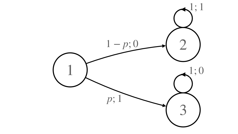
(b) Transition for action $a_{2}$

Figure 3: Transitions and rewards for a s-rectangular RMDP instance with no Blackwell optimal policy.

We can parametrize the return by the probability $x\in[0,1]$ to play action $a_{1}$ and by the parameter $p\in[0,1]$ chosen by the adversary. We have $R_{\gamma}(x,p)=xp\left(1+\frac{\gamma}{1-\gamma}\right)+(1-x)\left(p+(1-p)\frac{\gamma}{1-\gamma}\right).$ This can be reformulated $R_{\gamma}(x,p)=p\left(1+x\frac{\gamma}{1-\gamma}\right)+(1-p)\left((1-x)\frac{\gamma}{1-\gamma}\right).$ Let us compute the worst-case return for policy $x\in[0,1]$. We have $\min_{p\in[0,1]}R(x,p)=\min\{1+x\frac{\gamma}{1-\gamma},(1-x)\frac{\gamma}{1-\gamma}\}.$ The optimal policy then maximizes $x\mapsto\min_{p\in[0,1]}R(x,p)$, i.e., it maximizes $x\mapsto\min\{1+x\frac{\gamma}{1-\gamma},(1-x)\frac{\gamma}{1-\gamma}\}$ over $[0,1]$. Assume that $\gamma\geq 1/2$ (we are interested in Blackwell optimal policies, i.e. in the case $\gamma\rightarrow 1$). Then the maximum of $x\mapsto\min\{1+x\frac{\gamma}{1-\gamma},(1-x)\frac{\gamma}{1-\gamma}\}$ is attained at $x^{*}(\gamma)$, solution of the equation $1+x\frac{\gamma}{1-\gamma}=(1-x)\frac{\gamma}{1-\gamma}$. Therefore, there is a unique discount optimal policy and it depends on $\gamma$: $x^{\star}(\gamma)=1-\frac{1}{2\gamma}$ for $\gamma\geq 1/2$. Overall, no policies remain discount optimal when $\gamma$ varies, and there are no Blackwell optimal policies. ∎

We note that the counterexample in the proof of Proposition 4.22 is much simpler than the counterexample from Section 4.2.1 for sa-rectangular RMDPs. In particular, Proposition 4.22 shows that Blackwell optimal policies may fail to exist for s-rectangular RMDPs, even in the simple setting where the uncertainty set is a polytope parametrized by $p\in[0,1]$. As a possible next step, it sounds promising to study the existence and tractability of $\epsilon$-Blackwell optimal policies for s-rectangular RMDPs.

5 Algorithms

In this section, we discuss various iterative algorithms to compute average optimal and Blackwell optimal policies. Our results for s-rectangular RMDPs from Section 3.3 and Section 4.3 suggest that it may be difficult to compute average and Blackwell optimal policies in this case. Therefore, we focus on sa-rectangular robust MDPs. Since for sa-rectangular RMDPs an average optimal policy may be chosen stationary and deterministic, we define the optimal gain $\bm{g}^{\star}\in\mathbb{R}^{\mathcal{S}}$ as

$$g^{\star}_{s}=\max_{\pi\in\Pi_{\sf SD}}\inf_{\bm{P}\in\mathcal{U}}\lim_{T\rightarrow+\infty}\mathbb{E}_{\pi,\bm{P}}\left[\frac{1}{T+1}\sum_{t=0}^{T}r_{s_{t}a_{t}s_{t+1}}\;|\;s_{0}=s\right],\forall\;s\in\mathcal{S}.$$ (5.1)

We now introduce three algorithms to compute the optimal gain $\bm{g}^{\star}$ when $\mathcal{U}$ is sa-rectangular and definable.

5.1 Algorithms based on the Blackwell discount factor

As discussed in Section 4.2.3, when $\mathcal{U}$ is definable, we have shown that there exists a discount factor $\gamma_{{\sf bw}}\in(0,1)$, such that any policy that is $\gamma$-discount optimal for $\gamma\in(\gamma_{{\sf bw}},1)$ is also Blackwell optimal. Therefore, we can compute Blackwell optimal and average optimal policies by solving a sequence of discounted RMDPs with discount factors increasing to $1$. An immediate consequence is the following theorem.

Theorem 5.1

Let $\mathcal{U}$ be a definable compact convex uncertainty set and let $\left(\bm{v}^{t}\right)_{t\geq 1}$ and $\left(\pi^{t}\right)_{t\in\mathbb{N}}$ be the iterates of Algorithm 1. Then $\left(\bm{v}^{t}\right)_{t\geq 1}$ converges to $\bm{g}^{\star}\in\mathbb{R}^{\mathcal{S}}$, and $\pi^{t}$ is both Blackwell optimal and average optimal for $t\in\mathbb{N}$ large enough.

Unfortunately, computing the Blackwell discount factor $\gamma_{{\sf bw}}$ appears challenging, so that we are not able to provide a convergence rate for Algorithm 1. When $\mathcal{U}$ is polyhedral, Grand-Clément and Petrik (2023) obtains an upper bound on $\gamma_{{\sf bw}}$, but this upper bound is too close to $1$ to be of practical use. We also note that Algorithm 1 requires solving a robust MDP at every iteration, which may be computationally intensive. We now describe two algorithms with a lower per-iteration complexity.

Algorithm 1 Iterative algorithm for average optimality: limit of discounted values

Input: An increasing sequence of discount factors $\left(\gamma_{t}\right)_{t\in\mathbb{N}}$ with $\lim_{t\rightarrow+\infty}\gamma_{t}=1$.

Initialize $\bm{v}^{0}=\bm{0}\in\mathbb{R}^{\mathcal{S}},\pi^{0}\in\Pi_{\sf S}$.

for $t\in\mathbb{N}$ do

     $\bm{v}^{t+1}=(1-\gamma_{t})\bm{v}^{\star,\mathcal{U}}_{\gamma_{t}}$

     $\pi^{t+1}\in\Pi_{\sf S}$ such that $(1-\gamma_{t})\bm{v}^{\pi^{t+1},\mathcal{U}}_{\gamma_{t}}=\bm{v}^{t+1}$

end for

5.2 Algorithms based on value iteration

We now introduce two value iteration algorithms to compute the optimal worst-case average return when the uncertainty set $\mathcal{U}$ is definable.

Algorithm based on increasing horizon.

Algorithm 2 Iterative algorithm for average optimality: increasing horizon

Initialize $\bm{v}^{0}=\bm{0}\in\mathbb{R}^{\mathcal{S}}$.

for $t\in\mathbb{N}$ do

     $v^{t+1}_{s}=\max_{a\in\mathcal{A}}\min_{\bm{p}_{sa}\in\mathcal{U}_{sa}}\bm{p}_{sa}^{\top}\left(\bm{r}_{sa}+\bm{v}^{t}\right),\forall\;s\in\mathcal{S}$.

end for

We start with Algorithm 2, which computes the optimal value functions of a finite-horizon RMDP as the horizon increases to $+\infty$. The following theorem shows that Algorithm 2 is correct.

Theorem 5.2

Let $\mathcal{U}$ be a definable compact convex uncertainty set and let $\left(\bm{v}^{t}\right)_{t\geq 1}$ be the iterates of Algorithm 2. Then $\left(\frac{1}{t}\bm{v}^{t}\right)_{t\geq 1}$ converges to $\bm{g}^{\star}\in\mathbb{R}^{\mathcal{S}}$.

Proof.

Proof. When $\mathcal{U}$ is a definable uncertainty set, the same steps as Proposition 4.19 show that the robust Bellman operator (2.3) is definable. We also recall that we can cast a sa-rectangular RMDP as a perfect information SG. The authors in Bolte et al. (2015) show that when the operator of an SG is definable, then $\left(\frac{1}{t}\bm{v}^{t}\right)_{t\geq 1}$ admits a limit and that this limit coincides with $\lim_{\gamma\rightarrow 1}(1-\gamma)\bm{v}^{\star}_{\gamma}$ (see corollary 4, point (i), in Bolte et al. (2015)). We have shown in the third step of the proof of Theorem 4.6 that $\lim_{\gamma\rightarrow 1}(1-\gamma)\bm{p}_{0}^{\top}\bm{v}^{\star}_{\gamma}$ is equal to $\max_{\pi\in\Pi_{\sf SD}}\min_{\bm{P}\in\mathcal{U}}R_{{\sf avg}}(\pi,\bm{P})$. By definition of $\bm{g}^{\star}$, this shows that $\lim_{t\rightarrow+\infty}\frac{1}{t}\bm{v}^{t}=\bm{g}^{\star}$, which concludes the proof of Theorem 5.2. ∎

The proof of Theorem 5.2 is relatively short. This conciseness comes from invoking powerful results from the stochastic game literature (Bolte et al., 2015).

Algorithm based on increasing discount factor.

Algorithm 3 Iterative algorithm for average optimality: increasing discount factor

Input: an increasing sequence $\left(\omega_{t}\right)_{t\geq 0}\in\mathbb{R}^{\mathbb{N}}_{+}$ with $\lim_{t\rightarrow+\infty}\omega_{t}=+\infty,\lim_{t\rightarrow+\infty}\omega_{t}/\omega_{t+1}=1$.

Initialize $\bm{v}^{0}=\bm{0}\in\mathbb{R}^{\mathcal{S}}$.

for $t\in\mathbb{N}$ do

     $\gamma_{t}\;=\;\frac{\omega_{t}}{\omega_{t+1}}$

     $v^{t+1}_{s}\;=\;\max_{a\in\mathcal{A}}\min_{\bm{p}_{sa}\in\mathcal{U}_{sa}}\bm{p}_{sa}^{\top}\left((1-\gamma_{t})\bm{r}_{sa}+\gamma_{t}\bm{v}^{t}\right),\forall\;s\in\mathcal{S}$.

end for

We now consider Algorithm 3, which builds upon value iteration for RMDPs with an increasing sequence of discount factors. We have the following theorem.

Theorem 5.3

Let $\mathcal{U}$ be a definable compact convex uncertainty set and let $\left(\bm{v}^{t}\right)_{t\geq 1}$ be the iterates of Algorithm 3. Then $\left(\bm{v}^{t}\right)_{t\geq 1}$ converges to $\bm{g}^{\star}\in\mathbb{R}^{\mathcal{S}}$.

The proof of Theorem 5.3 is deferred to Appendix 20. We only provide the main steps here. The first step is to show the following lemma, which decomposes the suboptimality gap of the current iterates of Algorithm 1.

Lemma 5.4

There exist a period $t_{0}\in\mathbb{N}$ and two sequences of non-negative scalars $\left(\epsilon_{t}\right)_{t\geq t_{0}}$ and $\left(\delta_{t}\right)_{t\geq t_{0}}$ such that

$$\|\bm{v}^{t}-\bm{g}^{\star}\|_{\infty}\leq\epsilon_{t}+\delta_{t},\forall\;t\geq t_{0},$$

with $\lim_{t\rightarrow 0}\epsilon_{t}\rightarrow 0$ and with, for $t\geq t_{0}$ and $\pi^{B}$ a Blackwell optimal policy,

$$\delta_{t+1} =\gamma_{t}\delta_{t}+e_{t},$$ (5.2)

$$e_{t} =\|(1-\gamma_{t+1})\bm{v}^{\pi^{B},\mathcal{U}}_{\gamma_{t+1}}-(1-\gamma_{t})\bm{v}^{\pi^{B},\mathcal{U}}_{\gamma_{t}}\|_{\infty}.$$ (5.3)

The difficult part of the proof is to prove that the sequence $\left(\delta_{t}\right)_{t\geq t_{0}}$ converges to $0$. To show $\lim_{t\rightarrow+\infty}\delta_{t}\rightarrow 0$, we use the inductive step (5.2) and $\gamma_{t}=\omega_{t}/\omega_{t+1}$ to show

$$\delta_{t}=\frac{1}{\omega_{t+1}}\sum_{j=t_{0}}^{t}\omega_{j+1}e_{j},\forall\;t\geq t_{0}.$$ (5.4)

Equation (5.4) reveals that the expression of $\delta_{t}$ resembles a weighted Cesaro average of the sequence $\left(e_{t}\right)_{t\geq t_{0}}$. It is known that the Cesaro average of a converging sequence also converges to the same limit; we prove Theorem 5.3 by extending this result to weighted Cesaro averages and by invoking existing results from SGs to obtain that $\lim_{t\rightarrow+\infty}e_{t}=0.$

Comparison with previous work. We now compare Theorem 5.3 with related results from the RMDP literature. The authors in Tewari and Bartlett (2007) prove Theorem 5.3 with $\omega_{t}=t+1,$ i.e., with $\gamma_{t}=(t+1)/(t+2)$ and for the case of sa-rectangular uncertainty sets with $\ell_{\infty}$-balls. Tewari and Bartlett (2007) show the Lipschitz continuity of the robust value functions to simplify the term $e_{t}$ from Lemma 5.4. In particular, for sa-rectangular polyhedral $\mathcal{U}$, for $t$ large enough, there exists a constant $L>0$ such that

$$e_{t}=\|(1-\gamma_{t+1})\bm{v}^{\pi^{B},\mathcal{U}}_{\gamma_{t+1}}-(1-\gamma_{t})\bm{v}^{\pi^{B},\mathcal{U}}_{\gamma_{t}}\|_{\infty}\leq L\cdot\left(\gamma_{t+1}-\gamma_{t}\right).$$ (5.5)

Once (5.5) is established, one can conclude that

$$\delta_{t+1}=\gamma_{t}\delta_{t}+L\cdot\left(\gamma_{t+1}-\gamma_{t}\right)$$ (5.6)

and Lemma 8 in Tewari and Bartlett (2007) shows that a sequence $\left(\delta_{t}\right)_{t\geq 0}$ satisfying (5.6) converges to $0$.

The authors in Wang et al. (2023) consider Algorithm 3 with $\gamma_{t}=(t+1)/(t+2)$ for the case of general sa-rectangular uncertainty set (potentially non-polyhedral), with the assumption that the Markov chain associated with any transition probabilities and any policy is unichain. The analysis of Algorithm 3 in Wang et al. (2023) follows the same lines as the proof in Tewari and Bartlett (2007), and the authors conclude by claiming that the Lipschitzness property (5.5) holds for unichain RMDPs. The Lipschitnzess property for unichain RMDPs is claimed without a proof in Wang et al. (2023) and, in fact, in all generality the normalized robust value function $\gamma\mapsto(1-\gamma)\bm{v}^{\pi,\mathcal{U}}_{\gamma}$ may not be Lipschitz continuous for $\pi\in\Pi_{\sf S}$, as we prove in Appendix 19. We sidestep this issue by leveraging existing results from SGs (Bolte et al., 2015) and elementary results from real analysis.

Stopping criterion and complexity. We have proved that Algorithm 1, Algorithm 2, and Algorithm 3 converge to an optimal gain. However, we would like to emphasize that we do not introduce a stopping criterion for these algorithms. Even for the simpler case of nominal MDPs, in all generality, there is no known stopping criterion for value iteration for the average return criterion, e.g. Ashok et al. (2017) and section 9.4 in Puterman (2014). We leave finding a stopping criterion as an open question in this paper, noting that this is not addressed in previous papers on average-reward RMDPs (Tewari and Bartlett, 2007; Wang et al., 2023).

We also comment on the complexity of computing an average-optimal policy (and not just computing an optimal gain). For sa-rectangular RMDPs, this may be a difficult task. Indeed, we described the connections between sa-rectangular RMDPs with average return and mean-payoff perfect information stochastic games in Section 2.2. There is no known polynomial-time algorithm for solving this class of SGs (Condon, 1992; Zwick and Paterson, 1996; Andersson and Miltersen, 2009) even after more than six decades since their introduction in the game theory literature (Gillette, 1957), and this is regarded as one of the major open questions in algorithmic game theory. For this reason, in this paper, we have focused on the properties of average and Blackwell optimal policies and we leave designing polynomial-time algorithms for solving average return sa-rectangular RMDPs as an open question.

6 Numerical experiments

In this section, we compare the empirical performances of the algorithms introduced in Section 5. Our goal is to test the practical convergence of Algorithm 1, Algorithm 2 and Algorithm 3 on various sa-rectangular RMDPs instances.

Test instances. We consider three different nominal MDP instances: a machine replacement problem (Delage and Mannor, 2010; Wiesemann et al., 2013), a forest management instance (Possingham and Tuck, 1997; Cordwell et al., 2015), and an instance inspired from healthcare (Goyal and Grand-Clément, 2022). In the machine replacement problem, the goal is to compute a replacement and repair schedule for a line of machines. In the forest management instance, a forest grows at every period, and the goal is to balance the revenue from wood cutting and the risk of wildfire. In the healthcare instance, the goal is to plan the treatment of a patient, avoiding the mortality state while reducing the invasiveness of the treatment. We refer to the nominal transition probabilities in these instances as $\bm{P}_{\sf nom}$ and we represent the RMDP instances in Appendix 21.1.

Construction of the uncertainty sets. For each of these three RMDP instances, we consider two types of uncertainty sets. The first uncertainty set is based on box inequalities:

$$\mathcal{U}_{sa}^{\sf box}=\{\bm{p}\in\Delta(\mathcal{S})\;|\;\bm{p}_{sa}^{\sf low}\leq\bm{p}\leq\bm{p}_{sa}^{\sf up}\},\forall\;(s,a)\in\mathcal{S}\times\mathcal{A}$$

with $\bm{p}_{sa}^{\sf low},\bm{p}_{sa}^{\sf up}\in[0,1]^{\mathcal{S}}$ two vectors such that $\bm{p}_{sa}^{\sf low}\leq\bm{p}_{{\sf nom},sa}\leq\bm{p}_{sa}^{\sf up}$ for $(s,a)\in\mathcal{S}\times\mathcal{A}$. The second uncertainty set is based on ellipsoid constraints:

$$\mathcal{U}_{sa}^{\sf\ell_{2}}=\{\bm{p}\in\Delta(\mathcal{S})\;|\;\|\bm{p}-\bm{p}_{{\sf nom},sa}\|_{2}\leq\alpha\},\forall\;(s,a)\in\mathcal{S}\times\mathcal{A}$$

where $\alpha>0$ is a scalar. Box inequalities have been used in applications of RMDPs in healthcare (Goh et al., 2018), while uncertainty based on $\ell_{2}$-distance can be seen as conservative approximations of sets based on relative entropy (Iyengar, 2005). Note that both $\mathcal{U}^{\ell_{2}}$ and $\mathcal{U}^{\sf box}$ are definable sets, with $\mathcal{U}^{\sf box}$ being polyhedral. Additionally, there exist efficient algorithms to evaluate the robust Bellman operator as in (2.3) for $\mathcal{U}^{\sf box}$ (e.g. proposition 3 in Goh et al. (2018)). For $\mathcal{U}^{\sf\ell_{2}}$, evaluating the robust Bellman operator requires solving a convex program. Still, we can obtain a closed-form expression assuming that $\alpha>0$ is sufficiently small, as we detail in Appendix 21.2. We choose a uniform initial distribution for all instances.

Empirical setup. We run Algorithm 1, Algorithm 2 and Algorithm 3 for $T=50$ iterations, on the Machine, Forest, and Healthcare RMDP instances with $S=100$ states. For $\mathcal{U}^{\sf\ell_{2}}$ we choose a radius of $\alpha=0.05$ and for $\mathcal{U}^{\sf box}$ we choose the upper and lower bound on each coefficient to allow for $5\%$ deviations from the nominal distributions. For Algorithm 3, we choose $\omega_{t}=t+1$. We provide more details in Appendix 21.2. To implement Algorithm 1, we need to solve a robust MDP at every iteration. To do so, we implement the two-player strategy iteration (Hansen et al., 2013) with warm-starts, see more details in Appendix 21.3. We implement all algorithms in Python 3.8.8.

Numerical results. We first present the convergence rate as a function of the number of iterations of all our algorithms in Figure 4 for $\mathcal{U}^{\sf\ell_{2}}$ and in Figure 5 for $\mathcal{U}^{\sf box}$. Algorithm 1, Algorithm 2 and Algorithm 3 appear to have comparable convergence speed on our three RMDP instances, despite Algorithm 1 solving a discounted RMDP at each iteration, compared to Algorithm 2 and Algorithm 3 which only require to evaluate the robust Bellman operator. We also present the total computation time as a function of the number of iterations in Figure 6-7. We note that Algorithm 1 is much slower than Algorithm 2 and Algorithm 3, even with warm-start. Indeed, at every iteration, Algorithm 1 requires running two-player strategy iteration for solving a discounted RMDP, whereas the other two algorithms only require evaluating the Bellman operator. We also note that running our algorithms for $\mathcal{U}^{\sf\ell_{2}}$ is faster than for $\mathcal{U}^{\sf box}$, since the Bellman update for $\mathcal{U}^{\sf box}$ requires to sort a vector of size $|\mathcal{S}|$, and then compute a maximum, whereas for $\mathcal{U}^{\sf\ell_{2}}$ we only need to compute a maximum, see the implementation details in Appendix 21.2.

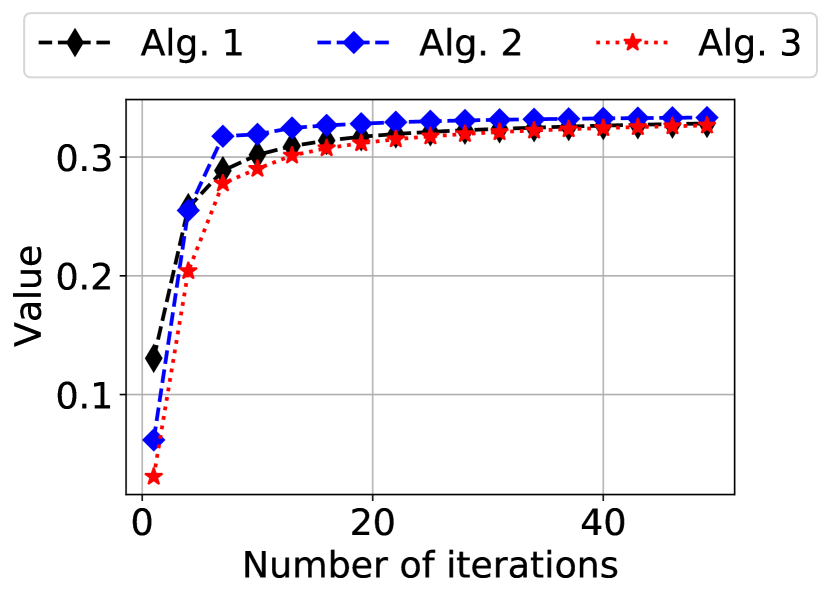
(a) Machine

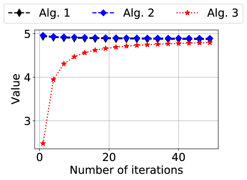
(b) Healthcare

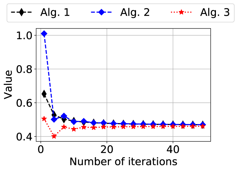
(c) Forest

Figure 4: Convergence to the optimal average return for various RMDP instances, for $\mathcal{U}^{\sf\ell_{2}}$ based on ellipsoids.

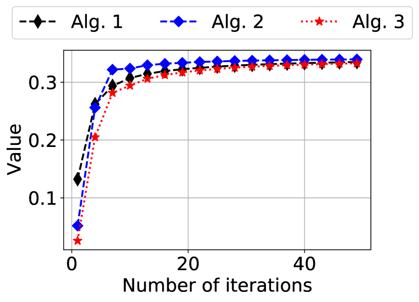
(a) Machine

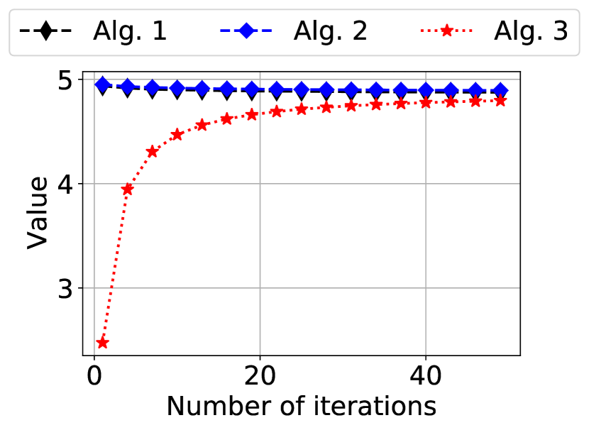
(b) Healthcare

(c) Forest

Figure 5: Convergence to the optimal average return for various RMDP instances, for $\mathcal{U}^{\sf box}$ based on box inequalities.

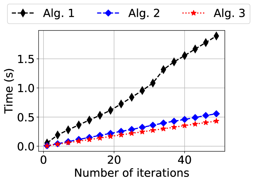
(a) Machine

(b) Healthcare

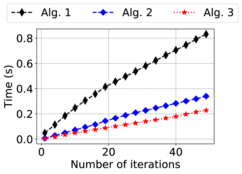
(c) Forest

Figure 6: Total computation time as a function of the number of iterations for various RMDP instances, for $\mathcal{U}^{\sf\ell_{2}}$ based on ellipsoids.

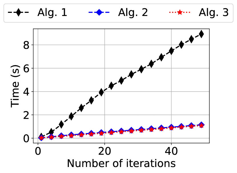
(a) Machine

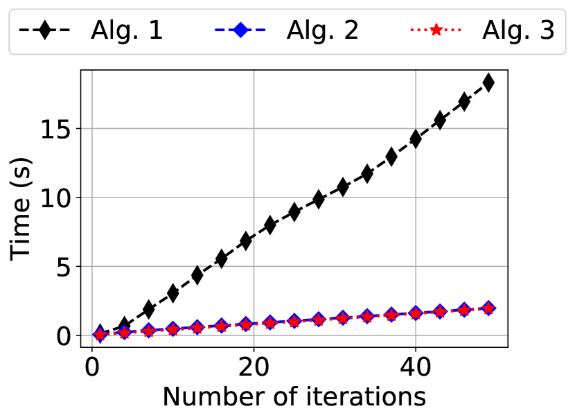
(b) Healthcare

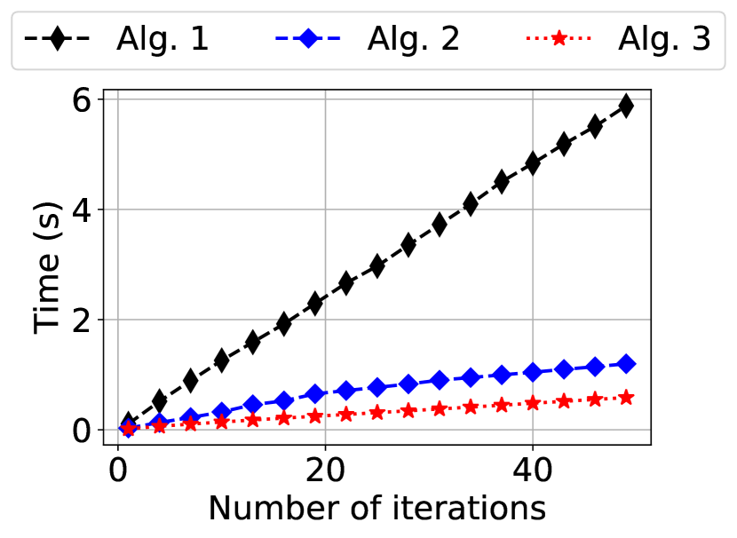
(c) Forest

Figure 7: Total computation time as a function of the number of iterations for various RMDP instances, for $\mathcal{U}^{\sf box}$ based on box inequalities.

7 Conclusion

Our paper addresses several important issues in the existing literature and derives the fundamental properties of average optimal and Blackwell optimal policies. In particular, our work highlights important distinctions between the widely-studied framework of discounted RMDPs and the less-studied frameworks of RMDPs with average optimality and Blackwell optimality. We view the non-existence of stationary average optimal policies for s-rectangular RMDPs and the non-existence of Blackwell optimal policies for sa-rectangular RMDPs (in all generality) as surprising results. The notion of definable uncertainty sets is also of independent interest, characterizing the cases where the value functions are well-behaved and iterative algorithms asymptotically converge to the optimal gain in the sa-rectangular case. Finally, our work opens new research avenues for RMDPs. Among them, deriving an efficient algorithm for computing an average optimal policy for sa-rectangular RMDPs appears crucial, but this may be difficult since a similar question remains open after several decades in the literature on SGs. Important other research questions include studying in more detail the particular case of irreducible instances, which considerably simplifies the main technical challenges, and studying the case of distributionally robust MDPs. Understanding if Markovian policies are sufficient for average return s-rectangular RMDPs also looks like a promising next direction.

8 Comparisons of SGs and RMDPs

In this section, we provide more details on the connections between perfect information stochastic games and sa-rectangular RMDPs. We refer to chapter 4 in Neyman et al. [2003] for a concise introduction to perfect information SGs. This class of games corresponds to SG instances where the state set $\Omega$ can be partitioned into two subsets $\Omega_{1},\Omega_{2}$ such that the first player entirely controls the states in $\Omega_{1}$ (in terms of instantaneous rewards and probabilities), and similarly for the second player for states in $\Omega_{2}$. We now briefly describe the reformulation of a sa-rectangular RMDP as a perfect information SG. We note that this construction is also described in section 5.2 in Goyal and Grand-Clément [2022] (without making the connection to stochastic games), in appendix A in Nilim and Ghaoui [2005] and in Section 5 in Iyengar [2005]. We provide the reformulation here for completeness.

Consider a sa-rectangular RMDP instance $\left(\mathcal{S},\mathcal{A},\bm{r},\mathcal{U},\bm{p}_{0}\right)$ with a convex set $\mathcal{U}$. We define a corresponding perfect information stochastic game instance as follows. The set of states is $\Omega=\Omega_{1}\cup\Omega_{2}$ with $\Omega_{1}=\mathcal{S},\Omega_{2}=\mathcal{S}\times\mathcal{A}$. The set of actions for the first player is $\mathcal{A}$, and the set of actions for the second player is the set of extreme points of $\mathcal{U}$. Note that with this construction, randomized strategies for the second player correspond to convex combinations of extreme points of the convex set $\mathcal{U}$, i.e., to elements of $\mathcal{U}$. There is no instantaneous payoff when visiting a state in $\Omega_{1}$, and there is an instantaneous payoff of $\bm{p}_{sa}^{\top}\bm{r}_{sa}$ in a state $(s,a)$ where the second player chooses $\bm{p}_{sa}\in\mathcal{U}_{sa}$. Given a state $\omega\in\Omega_{1}$, the transition function attributes a probability of $1$ to the next state $(s,a)\in\Omega_{2}$ if the first-player chooses action $a\in\mathcal{A}$ and $\omega=s$ for some $s\in\mathcal{S}$. Given a state $\omega\in\Omega_{2}$, the transition function attributes a probability of $p_{sas^{\prime}}$ to the next state $s^{\prime}\in\Omega_{1}$ if $\omega=(s,a)$ and the second player chooses action $\bm{p}_{sa}$. We represent this construction in Figure 8.

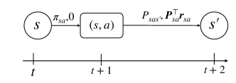
Figure 8: A sa-rectangular robust MDP as a perfect information game. The decision-maker controls the states $s\in\mathcal{S}$ and chooses an action $a\in\mathcal{A}$. The adversary controls the states $(s,a)\in\mathcal{S}\times\mathcal{A}$ and chooses transition probabilities $\bm{p}_{sa}\in\mathcal{U}_{sa}$. The pairs above the arcs represent the transition probabilities and instantaneous payoffs.

9 Proof of Proposition 2.2

Proof.

Proof of Proposition 2.2. Since $\mathcal{U}\subset\mathcal{U}_{\sf H}$, we always have $\sup_{\pi\in\Pi_{\sf H}}\inf_{\bm{P}\in\mathcal{U}_{\sf H}}R_{\gamma}(\pi,\bm{P})\leq\sup_{\pi\in\Pi_{\sf H}}\min_{\bm{P}\in\mathcal{U}}R_{\gamma}(\pi,\bm{P}).$ We now prove the converse inequality. We have

$$\sup_{\pi\in\Pi_{\sf H}}\min_{\bm{P}\in\mathcal{U}}R_{\gamma}(\pi,\bm{P}) \leq\min_{\bm{P}\in\mathcal{U}}\sup_{\pi\in\Pi_{\sf H}}R_{\gamma}(\pi,\bm{P})$$ (9.1)

$$=\min_{\bm{P}\in\mathcal{U}}\max_{\pi\in\Pi_{\sf S}}R_{\gamma}(\pi,\bm{P})$$ (9.2)

$$=\max_{\pi\in\Pi_{\sf S}}\min_{\bm{P}\in\mathcal{U}}R_{\gamma}(\pi,\bm{P})$$ (9.3)

$$=\max_{\pi\in\Pi_{\sf S}}\inf_{\bm{P}\in\mathcal{U}_{\sf H}}R_{\gamma}(\pi,\bm{P})$$ (9.4)

$$\leq\sup_{\pi\in\Pi_{\sf H}}\inf_{\bm{P}\in\mathcal{U}_{\sf H}}R_{\gamma}(\pi,\bm{P})$$ (9.5)

where (9.1) follows from weak duality, (9.2) follows from the inner maximization problem being an MDP, for which stationary optimal policies always exist [Puterman, 2014], (9.3) follows from strong duality for s-rectangular RMDPs, (9.4) follows from the inner minimization being an MDP (the adversarial MDP), see Goyal and Grand-Clément [2022], Ho et al. [2021]), and the last inequality following from $\Pi_{\sf S}\subset\Pi_{\sf H}.$ ∎

10 Detail on Example 3.1

Consider the following history-dependent (Markovian) policy $\pi$ such that at time $t\in\mathbb{N}$, $\pi$ chooses action $a_{0}$ if $2^{k}-1\leq t\leq 2\cdot(2^{k}-1)$ for some even integer $k\in\mathbb{N}$, or action $a_{1}$ otherwise. Intuitively, $\pi$ alternatively chooses $a_{0}$ and $a_{1}$, and the length of the interval where $\pi$ selects the same action doubles over time. Assume that the reward for choosing $a_{0}$ is $-1$ and the reward for choosing action $a_{1}$ is $1$. Let $T\in\mathbb{N}$. Then

$$\mathbb{E}_{\pi,\bm{P}}\left[\frac{1}{2^{T}-1}\sum_{t=0}^{2^{T}-2}r_{s_{t}a_{t}s_{t+1}}\;|\;s_{0}\sim\bm{p}_{0}\right]=\frac{1}{2^{T}-1}\sum_{k=0}^{T-1}\sum_{j=2^{k}-1}^{2\cdot(2^{k}-1)}(-1)^{k}=\frac{1}{2^{T}-1}\sum_{k=0}^{T-1}(-2)^{k}=\frac{1}{3}\times\frac{(-2)^{T}-1}{2^{T}-1}$$

from which we conclude that $\mathbb{E}_{\pi,\bm{P}}\left[\frac{1}{T+1}\sum_{t=0}^{T}r_{s_{t}a_{t}s_{t+1}}\;|\;s_{0}\sim\bm{p}_{0}\right]$ does not have a limit as $T\rightarrow+\infty$.

11 Some cases where the average worst-case transition probabilities exist

We have the following proposition.

Proposition 11.1

Let $\mathcal{U}$ be an s-rectangular compact convex robust MDP instance. Let $\pi\in\Pi_{\sf S}$. Then the infimum in $\inf_{\bm{P}\in\mathcal{U}}R_{{\sf avg}}(\pi,\bm{P})$ is attained under any of the following assumptions:

1. For any $(\pi,\bm{P})\in\Pi_{\sf S}\times\mathcal{U}$, the Markov chain induced by $(\pi,\bm{P})$ over $\mathcal{S}$ is unichain.

2. For any $(\pi,\bm{P})\in\Pi_{\sf S}\times\mathcal{U}$, the Markov chain induced by $(\pi,\bm{P})$ over $\mathcal{S}$ is irreducible.

3. The uncertainty set $\mathcal{U}$ is polyhedral.

Proof.

Proof. Under the first two assumptions, the average return $(\pi,\bm{P})\mapsto R_{{\sf avg}}(\pi,\bm{P})$ is continuous on $\Pi_{\sf S}\times\mathcal{U}$ (exercise 3, section 5.6, Filar and Vrieze [2012] and lemma 5.1.4, Filar and Vrieze [2012]). From Weierstrass theorem, $\bm{P}\mapsto R_{{\sf avg}}(\pi,\bm{P})$ attains its minimum over the compact set $\mathcal{U}$.

Under the assumption that $\mathcal{U}$ is polyhedral, we know that the worst-case transition probabilities (for a given $\pi\in\Pi_{\sf S}$) can be chosen in the set of extreme points of $\mathcal{U}$. Therefore, we can replace $\mathcal{U}$ by a finite set $\mathcal{U}_{\sf f}$ (its set of extreme points). Recall that the optimization problem $\inf_{\bm{P}\in\mathcal{U}}R_{{\sf avg}}(\pi,\bm{P})$ can be seen as the adversarial MDP [Ho et al., 2021]. In this MDP, the set of actions corresponds to $\mathcal{U}$. If we replace $\mathcal{U}$ by $\mathcal{U}_{\sf f}$, we obtain an MDP with finitely many actions. In this case, it is a classical result (see for instance chapter 8 and chapter 9 in Puterman [2014]) that a stationary deterministic policy is optimal for the average return, so that the infimum is attained in $\inf_{\bm{P}\in\mathcal{U}}R_{{\sf avg}}(\pi,\bm{P})$. ∎

12 Discussion on Lemma 3.3

In this appendix, we discuss the results in Bierth [1987]. In particular, the authors in Bierth [1987] focus on the case of nominal MDP with a finite set of states and compact action sets, where the rewards and the transitions are continuous in the chosen action. In this case, theorem 2.5 in Bierth [1987] shows that the worst-case average return over the set of history-dependent strategies is the same as the worst-case average return over the set of stationary deterministic strategies.

Recall that the adversarial MDP described in Section 2.1 has a finite set of states, a compact action set and continuous rewards and transitions. Therefore, we can use the results from theorem 2.5 in Bierth [1987] to obtain Lemma 3.3. The only difference is that we wrote Lemma 3.3 with an infimum over $\bm{P}\in\mathcal{U}$, which corresponds to stationary randomized policy of the adversary, whereas the conclusion of theorem 2.5 in Bierth [1987] pertains to stationary deterministic policies, which correspond to the set of extreme points of $\mathcal{U}$. We note that since ${\sf ext}(\mathcal{U})\subset\mathcal{U}\subset\mathcal{U}_{\sf H}$, Lemma 3.3 holds.

Remark 12.1

The authors in Wang et al. [2023] consider a statement equivalent to Lemma 3.3 for the case of Markovian adversary in unichain sa-rectangular RMDPs, see theorem 9 in Wang et al. [2023]. In particular, Wang et al. [2023] consider a stationary policy $\pi\in\Pi_{\sf S}$ and study the worst-case of the average return $\lim_{T\rightarrow+\infty}\mathbb{E}_{\pi,\bm{P}}\left[\frac{1}{T+1}\sum_{t=0}^{T}r_{s_{t}a_{t}s_{t+1}}\;|\;s_{0}\sim\bm{p}_{0}\right]$ over the set of Markovian adversary $\mathcal{U}_{\sf M}:=\mathcal{U}^{\mathbb{N}}$. However, we have shown in Example 3.1 that this limit may not exist when $\bm{P}\in\mathcal{U}_{\sf M}$, an issue that is overlooked in Wang et al. [2023]. We conclude by noting that Lemma 3.3 holds without the unichain assumption and that s-rectangularity is sufficient (instead of sa-rectangularity).

13 Proof of Theorem 3.5

Proof.

Proof of Theorem 3.5 We note that (3.5) is a consequence of (3.4). Indeed, if (3.4) holds, then

$$\inf_{\bm{P}\in\mathcal{U}}\max_{\pi\in\Pi_{\sf SD}}R_{{\sf avg}}(\pi,\bm{P})\leq\inf_{\bm{P}\in\mathcal{U}}\sup_{\pi\in\Pi_{\sf H}}R_{{\sf avg}}(\pi,\bm{P})=\sup_{\pi\in\Pi_{\sf H}}\inf_{\bm{P}\in\mathcal{U}}R_{{\sf avg}}(\pi,\bm{P})=\max_{\pi\in\Pi_{\sf SD}}\inf_{\bm{P}\in\mathcal{U}}R_{{\sf avg}}(\pi,\bm{P})$$

where the first inequality follows from $\Pi_{\sf SD}\subset\Pi_{\sf H}$ and the last equality follows from Theorem 3.4. We now dedicate our efforts to proving that (3.4) holds.

First, when $\mathcal{U}$ is polyhedral, we have

$$\inf_{\bm{P}\in\mathcal{U}}\sup_{\pi\in\Pi_{\sf H}}R_{{\sf avg}}(\pi,\bm{P})=\sup_{\pi\in\Pi_{\sf H}}\inf_{\bm{P}\in\mathcal{U}_{\sf H}}R_{{\sf avg}}(\pi,\bm{P})\leq\sup_{\pi\in\Pi_{\sf H}}\inf_{\bm{P}\in\mathcal{U}}R_{{\sf avg}}(\pi,\bm{P})$$

where the equality follows from (3.3) and the inequality follows from $\mathcal{U}\subset\mathcal{U}_{\sf H}$. This shows that (3.4) holds when $\mathcal{U}$ is polyhedral.

We now turn to showing (3.4) when $\mathcal{U}$ is a convex compact sa-rectangular uncertainty set. Let $\epsilon>0$ and consider the set $\mathcal{U}_{\sf f}$ defined similarly as in the second step of the proof of Theorem 3.4. We have

$$\inf_{\bm{P}\in\mathcal{U}}\sup_{\pi\in\Pi_{\sf H}}R_{{\sf avg}}(\pi,\bm{P}) \leq\inf_{\bm{P}\in\mathcal{U}_{\sf f}}\sup_{\pi\in\Pi_{\sf H}}R_{{\sf avg}}(\pi,\bm{P})$$ (13.1)

$$=\sup_{\pi\in\Pi_{\sf H}}\inf_{\bm{P}\in\mathcal{U}_{\sf f}}R_{{\sf avg}}(\pi,\bm{P})$$ (13.2)

$$=\max_{\pi\in\Pi_{\sf SD}}\inf_{\bm{P}\in\mathcal{U}_{\sf f}}R_{{\sf avg}}(\pi,\bm{P})$$ (13.3)

$$\leq\max_{\pi\in\Pi_{\sf SD}}\inf_{\bm{P}\in\mathcal{U}}R_{{\sf avg}}(\pi,\bm{P})+\epsilon$$ (13.4)

$$=\sup_{\pi\in\Pi_{\sf H}}\inf_{\bm{P}\in\mathcal{U}}R_{{\sf avg}}(\pi,\bm{P})+\epsilon$$ (13.5)

where (13.1) follows from $\mathcal{U}_{\sf f}\subset\mathcal{U}$, (13.2) follows from the first two steps of this proof and $\mathcal{U}_{\sf f}$ having only finitely many extreme points, (13.3) follows from Theorem 3.4, (13.4) follows from the construction of $\mathcal{U}_{\sf f}$, and (13.5) follows from Theorem 3.4 again. Since the inequalities above are true for any choice of $\epsilon>0$, we conclude that $\sup_{\pi\in\Pi_{\sf H}}\inf_{\bm{P}\in\mathcal{U}}R_{{\sf avg}}(\pi,\bm{P})=\inf_{\bm{P}\in\mathcal{U}}\sup_{\pi\in\Pi_{\sf H}}R_{{\sf avg}}(\pi,\bm{P}).$ ∎

14 Proof of Corollary 3.7

Proof.

Proof of Corollary 3.7. The proof proceeds in three parts. Let $\hat{R}_{{\sf avg}}$ as defined in (3.6), (3.7), or (3.8).

Part 1. Crucially, for any $(\pi,\bm{P})\in\Pi_{\sf H}\times\mathcal{U}$,

$$\hat{R}_{{\sf avg}}(\pi,\bm{P})\leq R_{{\sf avg}}(\pi,\bm{P})$$ (14.1)

and $\hat{R}_{{\sf avg}}(\pi,\bm{P})=R_{{\sf avg}}(\pi,\bm{P})$ when $(\pi,\bm{P})\in\Pi_{\sf S}\times\mathcal{U}$. From this, we have

$$\max_{\pi\in\Pi_{\sf SD}}\inf_{\bm{P}\in\mathcal{U}}\hat{R}_{{\sf avg}}(\pi,\bm{P})=\max_{\pi\in\Pi_{\sf SD}}\inf_{\bm{P}\in\mathcal{U}}R_{{\sf avg}}(\pi,\bm{P})=\sup_{\pi\in\Pi_{\sf H}}\inf_{\bm{P}\in\mathcal{U}}R_{{\sf avg}}(\pi,\bm{P})\geq\sup_{\pi\in\Pi_{\sf H}}\inf_{\bm{P}\in\mathcal{U}}\hat{R}_{{\sf avg}}(\pi,\bm{P})$$

where the first equality holds from the optimization variables $(\pi,\bm{P})$ being in $\Pi_{\sf SD}\times\mathcal{U}$, the second equality holds from the first step of the proof, and the inequality follows from (14.1). This shows that when $\hat{R}_{{\sf avg}}$ is defined as in (3.6), (3.7), or (3.8), we have $\sup_{\pi\in\Pi_{\sf H}}\inf_{\bm{P}\in\mathcal{U}}\hat{R}_{{\sf avg}}(\pi,\bm{P})=\max_{\pi\in\Pi_{\sf SD}}\inf_{\bm{P}\in\mathcal{U}}\hat{R}_{{\sf avg}}(\pi,\bm{P}).$ Now since $\hat{R}_{{\sf avg}}$ and $R_{{\sf avg}}$ coincides over $\Pi_{\sf S}\times\mathcal{U}$, we can conclude that $\max_{\pi\in\Pi_{\sf SD}}\inf_{\bm{P}\in\mathcal{U}}\hat{R}_{{\sf avg}}(\pi,\bm{P})=\max_{\pi\in\Pi_{\sf SD}}\inf_{\bm{P}\in\mathcal{U}}R_{{\sf avg}}(\pi,\bm{P})$.

Part 2. We now turn to proving that the following strong duality results hold:

$$\sup_{\pi\in\Pi_{\sf H}}\inf_{\bm{P}\in\mathcal{U}}\hat{R}_{{\sf avg}}(\pi,\bm{P}) =\inf_{\bm{P}\in\mathcal{U}}\sup_{\pi\in\Pi_{\sf H}}\hat{R}_{{\sf avg}}(\pi,\bm{P})$$ (14.2)

$$\max_{\pi\in\Pi_{\sf SD}}\inf_{\bm{P}\in\mathcal{U}}\hat{R}_{{\sf avg}}(\pi,\bm{P}) =\inf_{\bm{P}\in\mathcal{U}}\max_{\pi\in\Pi_{\sf SD}}\hat{R}_{{\sf avg}}(\pi,\bm{P})$$ (14.3)

Similarly as for the proof of Theorem 3.5, it is sufficient to show(14.2). We have

$$\inf_{\bm{P}\in\mathcal{U}}\sup_{\pi\in\Pi_{\sf H}}\hat{R}_{{\sf avg}}(\pi,\bm{P}) \leq\inf_{\bm{P}\in\mathcal{U}}\sup_{\pi\in\Pi_{\sf H}}R_{{\sf avg}}(\pi,\bm{P})$$ (14.4)

$$=\sup_{\pi\in\Pi_{\sf H}}\inf_{\bm{P}\in\mathcal{U}}R_{{\sf avg}}(\pi,\bm{P})$$ (14.5)

$$=\max_{\pi\in\Pi_{\sf SD}}\inf_{\bm{P}\in\mathcal{U}}R_{{\sf avg}}(\pi,\bm{P})$$ (14.6)

$$\leq\max_{\pi\in\Pi_{\sf SD}}\inf_{\bm{P}\in\mathcal{U}}\hat{R}_{{\sf avg}}(\pi,\bm{P})$$ (14.7)

$$\leq\sup_{\pi\in\Pi_{\sf H}}\inf_{\bm{P}\in\mathcal{U}}\hat{R}_{{\sf avg}}(\pi,\bm{P})$$ (14.8)

where (14.4) follows from $\hat{R}_{{\sf avg}}(\pi,\bm{P})\leq R_{{\sf avg}}(\pi,\bm{P})$ for $(\pi,\bm{P})\in\Pi_{\sf H}\times\mathcal{U}$, (14.5) follows from Theorem 3.5, (14.6) follows from Theorem 3.4, (14.7) follows from $\hat{R}_{{\sf avg}}(\pi,\bm{P})=R_{{\sf avg}}(\pi,\bm{P})$ for $(\pi,\bm{P})\in\Pi_{\sf S}\times\mathcal{U}$, and (14.8) follows from $\mathcal{U}_{\sf SD}\subset\mathcal{U}_{\sf H}$. Therefore, $\sup_{\pi\in\Pi_{\sf H}}\inf_{\bm{P}\in\mathcal{U}}\hat{R}_{{\sf avg}}(\pi,\bm{P})=\inf_{\bm{P}\in\mathcal{U}}\sup_{\pi\in\Pi_{\sf H}}\hat{R}_{{\sf avg}}(\pi,\bm{P}).$

Part 3. Finally, we prove that Theorem 3.6 still holds for $\hat{R}_{{\sf avg}}$, i.e. we show that

$$\sup_{\pi\in\Pi_{\sf H}}\inf_{\bm{P}\in\mathcal{U}}\hat{R}_{{\sf avg}}(\pi,\bm{P})=\sup_{\pi\in\Pi_{\sf H}}\inf_{\bm{P}\in\mathcal{U}_{H}}\hat{R}_{{\sf avg}}(\pi,\bm{P}).$$

Note that proof for Theorem 3.6 only relies on Theorem 3.4, Theorem 3.5 and Lemma 3.3. We have proved above that Theorem 3.4 and Theorem 3.5 still hold when we replace $\hat{R}_{{\sf avg}}$ by $R_{{\sf avg}}$. The authors in Bierth [1987] also prove Lemma 3.3 for $\hat{R}_{{\sf avg}}$ as in (3.6), (3.7), or (3.8). Therefore, the proof of Theorem 3.6 follows verbatim when replacing $R_{{\sf avg}}$ by $\hat{R}_{{\sf avg}}$. ∎

15 Proof of Theorem 4.4

We consider the following sa-rectangular robust MDP instance, which builds upon the counterexample for Proposition 3.2. There are three states $\{s_{0},s_{1},s_{2}\}$, where $s_{1}$ is an absorbing state with reward $-1$ and $s_{2}$ is an absorbing state with reward $0$. The decision-maker starts in state $s_{0}$ with probability $1$. The instantaneous reward in $s_{0}$ is $0$. There are two actions $\{a_{1},a_{2}\}$, and for $i\in\{1,2\}$,

$$\mathcal{U}_{s_{0}a_{i}}=\{\left(1-\alpha,\beta,\alpha-\beta\right)\;|\;\alpha\in[0,1],\beta\in[0,\alpha],\beta\leq D_{i}(\alpha)\}$$

for $D_{1}$ and $D_{2}$ two concave functions such that $D_{1}(\alpha)\leq\alpha,D_{2}(\alpha)\leq\alpha.$ We will specify $D_{1}$ and $D_{2}$ later. For a vector $\left(1-\alpha,\beta,\alpha-\beta\right)$ in the simplex, we can interpret $\alpha$ as the probability to leave state $s_{0}$ and $\beta$ as the probability to go to state $s_{1}$. This is represented in Figure 1(a). Since state $s_{0}$ is the only non-absorbing state, we can identify policies and the action ($a_{1}$ or $a_{2}$) chosen at $s_{0}$. Since we are considering a sa-rectangular robust MDP, for every discount factor $\gamma\in(0,1)$ there is a deterministic stationary optimal policy in $\{a_{1},a_{2}\}$. The worst-case return of $a_{1}$ and $a_{2}$ are defined as, for $i\in\{1,2\}$

$$R_{\gamma}(a_{i}):=\min_{\bm{P}\in\mathcal{U}}R_{\gamma}(a_{i},\bm{P})=\frac{1}{1-\gamma}\min_{\alpha\in[0,1],\beta\in[0,\alpha],\left(1-\alpha,\beta,\alpha-\beta\right)\in\mathcal{U}_{sa_{i}}}-\gamma\frac{\beta}{1-\gamma+\gamma\alpha}.$$

From the definition of $\mathcal{U}_{sa_{i}}$ for $i\in\{1,2\}$, we can write $R_{\gamma}(a_{i})$ as

$$R_{\gamma}(a_{i})=-\frac{1}{1-\gamma}\max_{\alpha\in[0,1]}\;\gamma\frac{D_{i}(\alpha)}{1-\gamma+\gamma\alpha}.$$

We will construct two sequences $\left(\gamma_{k}\right)_{k\in\mathbb{N}}$ and $\left(\gamma^{\prime}_{k}\right)_{k\in\mathbb{N}}$ such that for any $k\in\mathbb{N}$, $a_{1}$ is the unique optimal policy for $\gamma=\gamma_{k}$ and $a_{2}$ is the unique optimal policy for $\gamma=\gamma^{\prime}_{k}$, and $\gamma_{k}\rightarrow 1,\gamma^{\prime}_{k}\rightarrow 1$ as $k\rightarrow+\infty$.

First step.

We first consider the following function $D:[0,1]\rightarrow[0,1]$ defined as $D(\alpha)=\alpha(1-\alpha)$, and consider the following optimization program:

$$\max_{\alpha\in[0,1]}\;\gamma\frac{D(\alpha)}{1-\gamma+\gamma\alpha}=\max_{\alpha\in[0,1]}\;\gamma\frac{\alpha(1-\alpha)}{1-\gamma+\gamma\alpha}.$$

The derivative of $\alpha\mapsto\frac{\alpha(1-\alpha)}{1-\gamma+\gamma\alpha}$ is $\frac{(1-2\alpha)(1-\gamma+\gamma\alpha)-\alpha(1-\alpha)\gamma}{(1-\gamma+\gamma\alpha)^{2}}=\frac{1-\gamma-2\alpha(1-\gamma)-\gamma\alpha^{2}}{(1-\gamma+\gamma\alpha)^{2}},$ which shows that the maximum of $\alpha\mapsto\frac{\alpha(1-\alpha)}{1-\gamma+\gamma\alpha}$ is attained at $\alpha^{\star}(\gamma)=\frac{\sqrt{1-\gamma}-(1-\gamma)}{\gamma}$. Note that $\gamma\mapsto\alpha^{\star}(\gamma)$ is a decreasing function on $(0,1]$ that we can continuously extend to $[0,1]$, with $\alpha^{\star}(1)=0$ and $\alpha^{\star}(0)=1/2$.

Second step.

We now construct two piece-wise affine functions $D_{1},D_{2}$, that are (pointwise) smaller than $D:\alpha\mapsto\alpha(1-\alpha)$ on $[0,1]$ , and that intersect infinitely many times on any interval $(0,\alpha_{0})$ for any $\alpha_{0}\in(0,1/2).$ In particular, we have the following lemma. We call breakpoints of a piecewise affine function the points where it changes slopes.

Lemma 15.1

Let $D_{1}:[0,1]\rightarrow\mathbb{R},D_{2}:[0,1]\rightarrow\mathbb{R}$ defined as follows.

1. $D_{1}$ is piecewisewise affine, its set of breakpoints is $\{\frac{1}{2k}\;|\;k\geq 1\}$, where $D_{1}(\frac{1}{2k})=D(\frac{1}{2k}),k\geq 1$.

2. $D_{2}$ is piecewisewise affine, its set of breakpoints is $\{\frac{1}{2k+1}\;|\;k\geq 1\}$, where $D_{2}(\frac{1}{2k+1})=D(\frac{1}{2k+1}),k\geq 1$.

Then $D_{1},D_{2}$ are continuous, concave, and increasing functions on $[0,1/2]$. Additionally, $D_{1}$ and $D_{2}$ intersect infinitely many times on any interval $(0,\alpha_{0})$ with $\alpha_{0}\in(0,1/2)$.

Proof.

Proof of Lemma 15.1. We first show that $D_{1}$ is a concave, strictly increasing function. For $k\geq 1$ and $x\in\left(\frac{1}{2k+2},\frac{1}{2k}\right)$, there exists $a_{1,k},b_{1,k}\in\mathbb{R}$ such that $D_{1}(x)=a_{1,k}x+b_{1,k}$. In particular, we have

$$a_{1,k}=\frac{D_{1}\left(\frac{1}{2k}\right)-D_{1}\left(\frac{1}{2k+1}\right)}{\frac{1}{2k}-\frac{1}{2k+2}}=\frac{\frac{1}{2k}\left(1-\frac{1}{2k}\right)-\frac{1}{2k+2}\left(1-\frac{1}{2k+2}\right)}{\frac{1}{2k}-\frac{1}{2k+2}}=\frac{2k^{2}-1}{2k^{2}+2k}.$$

We also have $a_{1,k}\frac{1}{2k}+b_{1,k}=D_{1}\left(\frac{1}{2k}\right)$, so that $b_{1,k}=\frac{1}{4k(k+1)}.$ Note that $k\mapsto\frac{2k^{2}-1}{2k^{2}+2k}$ is an increasing function, with $\lim_{k\rightarrow+\infty}\frac{2k^{2}-1}{2k^{2}+2k}=1.$ Therefore, we have shown that $k\mapsto a_{1,k}$ is an increasing function. Since $D_{1}$ is continuous by construction, we conclude that $D_{1}$ is a concave, increasing function. The same approach shows that $D_{2}$ is concave and strictly increasing.

We now show that the two functions intersect infinitely many times on any interval $(0,\alpha_{0})$ with $\alpha_{0}>0$. Let $k\geq 1$. Then there is a zero of $x\mapsto D_{1}(x)-D_{2}(x)$ on any interval $\left(\frac{1}{k+1},\frac{1}{k}\right)$. From the concavity of $x\mapsto\sqrt{x}$, we have that $D_{2}\left(\frac{1}{2k+1}\right)-D_{1}\left(\frac{1}{2k+1}\right)\geq 0$ and $D_{2}\left(\frac{1}{2k+2}\right)-D_{1}\left(\frac{1}{2k+2}\right)\leq 0$. Since $D_{1},D_{2}$ are continuous, there exists a zero of $x\mapsto D_{1}(x)-D_{2}(x)$ on any interval $\left(\frac{1}{2k+2},\frac{1}{2k+1}\right)$ for $k\geq 1$. The same approach shows that there exists a zero $x\mapsto D_{1}(x)-D_{2}(x)$ on any interval $\left(\frac{1}{2k+1},\frac{1}{2k}\right)$ for $k\geq 1$. ∎

Third step.

We now construct a sequence of discount factors $\left(\gamma_{k}\right)_{k\in\mathbb{N}}$ such that $\gamma_{k}\rightarrow 1$ and $a_{1}$ is the unique optimal policy for $\gamma=\gamma_{k}$ for any $k\in\mathbb{N}$. Let $k\in\mathbb{N}$ and $\gamma_{k}\in(0,1)$ such that $\alpha^{\star}(\gamma_{k})=\frac{1}{2k+1}$. From the strict monotonicity of $\gamma\mapsto\alpha^{\star}(\gamma)$ we know that $\gamma_{k}\rightarrow 1$ as $k\rightarrow+\infty$. By construction,

$$R_{\gamma_{k}}(a_{2}) =-\frac{1}{1-\gamma_{k}}\max_{\alpha\in[0,1]}\frac{D_{2}(\alpha)}{1-\gamma_{k}+\gamma_{k}\alpha}$$

$$\geq-\frac{1}{1-\gamma_{k}}\max_{\alpha\in[0,1]}\frac{D(\alpha)}{1-\gamma_{k}+\gamma_{k}\alpha}$$ (15.1)

$$=-\frac{1}{1-\gamma_{k}}\frac{D(\frac{1}{2k+1})}{1-\gamma_{k}+\gamma_{k}\frac{1}{2k+1}}$$ (15.2)

$$=-\frac{1}{1-\gamma_{k}}\frac{D_{2}(\frac{1}{2k+1})}{1-\gamma_{k}+\gamma_{k}\frac{1}{2k+1}}$$ (15.3)

where (15.1) follows from $D_{2}(\alpha)\leq D(\alpha)$ for any $\alpha\in(0,1/2)$, where (15.2) follows from the definition of $\gamma_{k}$ such that $\alpha^{\star}(\gamma_{k})=\frac{1}{2k+1}$, and (15.3) follows from $D_{2}(\frac{1}{2k+1})=D(\frac{1}{2k+1})$ by construction of $D_{2}$ as in Lemma 15.1. This shows that the maximum in $R_{\gamma_{k}}(a_{2})$ is attained at $\alpha^{\star}(\gamma_{k})=\frac{1}{2k+1}$.

We now show that $R_{\gamma_{k}}(a_{1})>R_{\gamma_{k}}(a_{2})$. The function $\alpha\mapsto\frac{D_{1}(\alpha)}{1-\gamma_{k}+\gamma_{k}\alpha}$ is continuous on the compact set $[0,1/2]$, hence it attains its maximum. We distinguish two cases.

Case 1. Suppose that this maximum is attained at $\alpha_{1}\in\{1/2k^{\prime}\;|\;k^{\prime}\in\mathbb{N}\}$. Then $D_{1}(\alpha_{1})=D(\alpha_{1})$, and

$$\frac{D_{1}(\alpha_{1})}{1-\gamma_{k}+\gamma_{k}\alpha_{1}}=\frac{D(\alpha_{1})}{1-\gamma_{k}+\gamma_{k}\alpha_{1}}<\max_{\alpha\in[0,1/2]}\frac{D(\alpha_{1})}{1-\gamma_{k}+\gamma_{k}\alpha_{1}}$$

where the strict inequality follows from $\alpha^{\star}(\gamma_{k})=1/(2k+1)\neq\alpha_{1}.$

Case 2. Otherwise, the maximum of $\alpha\mapsto\frac{D_{1}(\alpha)}{1-\gamma_{k}+\gamma_{k}\alpha}$ is attained at $\alpha_{1}\notin[0,1/2]$ but $\alpha_{1}\notin\{1/2k^{\prime}\;|\;k^{\prime}\in\mathbb{N}\}$. In this case we have by construction that $D_{1}(\alpha_{1})<D(\alpha_{1})$ so that

$$\frac{D_{1}(\alpha_{1})}{1-\gamma_{k}+\gamma_{k}\alpha_{1}}<\frac{D(\alpha_{1})}{1-\gamma_{k}+\gamma_{k}\alpha_{1}}\leq\max_{\alpha\in[0,1/2]}\frac{D(\alpha_{1})}{1-\gamma_{k}+\gamma_{k}\alpha_{1}}.$$

Overall, we conclude that $R_{\gamma_{k}}(a_{1})>R_{\gamma_{k}}(a_{2})$ in both case $1$ and case $2$. Threfore, we have constructed a sequence $\left(\gamma_{k}\right)_{k\in\mathbb{N}}$ such that $R_{\gamma_{k}}(a_{1})>R_{\gamma_{k}}(a_{2}),\forall\;k\geq 1$. The construction of a sequence $\left(\gamma_{k}^{\prime}\right)_{k\in\mathbb{N}}$ such that $R_{\gamma_{k}^{\prime}}(a_{1})>R_{\gamma_{k}^{\prime}}(a_{2}),\forall\;k\geq 1$ is analogous, by choosing $\gamma^{\prime}_{k}$ such that $\alpha^{\star}(\gamma^{\prime}_{k})=\frac{1}{2k}$. This shows that there does not exist a stationary deterministic Blackwell optimal policy. Since for any $k\in\mathbb{N}$, at $\gamma=\gamma_{k}$ there is a unique discount optimal policy and it is stationary deterministic, this shows that there does not exist a Blackwell optimal policy that is history-dependent. This concludes the construction of our counterexample.

Remark 15.2

Wang et al. [2023] show the existence of a stationary deterministic Blackwell optimal policy for sa-rectangular RMDPs, under two conditions: (a) the Markov chains induced by any pair of policy and transition probabilities are unichain, (b) there is a unique average optimal policy. The second assumption precludes two value functions from intersecting infinitely often as $\gamma\rightarrow 1$, which is exactly the problematic behavior in our counterexample. In fact, our counterexample violates both assumptions: there are two absorbing states (which violates the unichain assumption), and actions $a_{1}$ and $a_{2}$ are average optimal.

16 Proof of Theorem 4.5

Proof.

Proof of Theorem 4.5.

We first fix a stationary policy $\pi\in\Pi_{\sf S}$ and a discount factor $\gamma\in(0,1)$. Theorem 4.3 shows that for each $\epsilon>0$ and each policy $\pi\in\Pi_{\sf S}$, there exists an $\epsilon$-Blackwell optimal policy for the adversarial MDP. In particular, for each $\epsilon>0$ and each policy $\pi\in\Pi_{\sf S}$, there exists a transition probability matrix $\bm{P}^{\pi}_{\epsilon}\in\mathcal{U}$ and a discount factor $\gamma^{\pi}_{\epsilon}\in(0,1),$ such that

$$(1-\gamma)\left(v^{\pi,\bm{P}^{\pi}_{\epsilon}}_{\gamma,s}-v^{\pi,\mathcal{U}}_{\gamma,s}\right)\leq\epsilon,\quad\forall\;\gamma>\gamma^{\pi}_{\epsilon},\forall\;s\in\mathcal{S}.$$

Assume a fixed $\epsilon>0$. For any discount factor $\gamma\in(0,1)$ consider the set $\{R_{\gamma}(\pi,\bm{P}^{\pi}_{\epsilon/2})\;|\;\pi\in\Pi_{\sf SD}\}$. This set is finite since $\pi\in\Pi_{\sf SD}$ is finite. We then define $\hat{\pi}_{\gamma}\in\arg\max_{\pi\in\Pi_{\sf SD}}R_{\gamma}(\pi,\bm{P}^{\pi}_{\epsilon/2})$ Since $\hat{\pi}_{\gamma}\in\Pi_{\sf SD},\forall\;\gamma\in(0,1)$ and $\Pi_{\sf SD}$ is finite, we can choose a sequence of discount factors $\left(\gamma_{n}\right)_{n\geq 1}$ such that for all $n\in\mathbb{N}$, we have $\hat{\pi}_{\gamma_{n}}=\pi\in\Pi_{\sf SD}$ for some $\pi\in\Pi_{\sf SD}$ and $\gamma_{n}\rightarrow 1$ as $n\rightarrow+\infty$ (see for instance lemma F.1 in Goyal and Grand-Clément [2022]). Next, we show that the policy $\pi$ is $\epsilon$-Blackwell optimal.

Indeed, suppose that $\pi$ is not $\epsilon$-Blackwell optimal: we can construct a sequence of discount factors $\left(\gamma^{\prime}_{n}\right)_{n\in\mathbb{N}}\in(0,1)^{\mathbb{N}}$ and a sequence of states $\left(s_{n}\right)_{n\in\mathbb{N}}\in\mathcal{S}^{\mathbb{N}}$ such that $(1-\gamma^{\prime}_{n})\left(v^{\star,\mathcal{U}}_{\gamma^{\prime}_{n},s_{n}}-v^{\pi,\mathcal{U}}_{\gamma^{\prime}_{n},s_{n}}\right)>\epsilon,\forall\;n\geq 1.$ and $\gamma^{\prime}_{n}\rightarrow 1$ as $n\rightarrow+\infty$. Since for each $\gamma^{\prime}_{n}$ the optimal discount policy can be chosen stationary and deterministic, i.e., in $\Pi_{\sf SD}$, we can find a policy $\pi^{\prime}$ and a state $s\in\mathcal{S}$ such that $(1-\gamma^{\prime}_{n})\left(v^{\pi^{\prime},\mathcal{U}}_{\gamma^{\prime}_{n},s}-v^{\pi,\mathcal{U}}_{\gamma^{\prime}_{n},s}\right)>\epsilon,\forall\;n\geq 1.$ By definition of the transition probabilities $\bm{P}^{\pi}_{\epsilon/2}$ and $\bm{P}^{\pi^{\prime}}_{\epsilon/2}$ we have

$$(1-\gamma)\left(v^{\pi^{\prime},\bm{P}^{\pi^{\prime}}_{\epsilon/2}}_{\gamma,s}-v^{\pi^{\prime},\mathcal{U}}_{\gamma,s}\right)\leq\epsilon/2,\quad\forall\;\gamma>\gamma^{\pi^{\prime}}_{\epsilon/2},$$

$$(1-\gamma)\left(v^{\pi,\bm{P}^{\pi}_{\epsilon/2}}_{\gamma,s}-v^{\pi,\mathcal{U}}_{\gamma,s}\right)\leq\epsilon/2,\quad\forall\;\gamma>\gamma^{\pi}_{\epsilon/2}.$$

Since $\gamma^{\prime}_{n}\rightarrow 1$ as $n\rightarrow+\infty$, we conclude that for some $n_{0}\in\mathbb{N}$ we have

$$(1-\gamma^{\prime}_{n})\left(v^{\pi^{\prime},\bm{P}^{\pi^{\prime}}_{\epsilon/2}}_{\gamma^{\prime}_{n},s}-v^{\pi,\bm{P}^{\pi}_{\epsilon/2}}_{\gamma^{\prime}_{n},s}\right)>\epsilon/2>0,\forall\;n\geq n_{0}.$$ (16.1)

But by construction of $\pi$, we have $\pi\in\arg\max_{\hat{\pi}\in\Pi_{\sf SD}}v^{\hat{\pi},\bm{P}^{\hat{\pi}}_{\epsilon/2}}_{\gamma_{n}},\forall\;n\geq 1.$ From this we conclude that

$$v^{\pi^{\prime},\bm{P}^{\pi^{\prime}}_{\epsilon/2}}_{\gamma_{n},s}-v^{\pi,\bm{P}^{\pi}_{\epsilon/2}}_{\gamma_{n},s}\leq 0,\forall\;n\geq n_{0}.$$ (16.2)

Combining (16.1) and (16.2), we obtain that $\gamma\mapsto v^{\pi^{\prime},\bm{P}^{\pi^{\prime}}_{\epsilon/2}}_{\gamma,s}-v^{\pi,\bm{P}^{\pi}_{\epsilon/2}}_{\gamma,s}$ must cancel infinitely many times in the interval $(0,1)$, which is a contradiction since this is a rational function (lemma 10.1.3, Puterman [2014]). Therefore, for any $\epsilon>0$ we can choose $\pi_{\epsilon}\in\Pi_{\sf SD}$ that is $\epsilon$-Blackwell optimal. Since $\Pi_{\sf SD}$ is finite, the same stationary deterministic policy can be chosen $\epsilon$-Blackwell optimal for all $\epsilon>0$. ∎

17 Proof of Theorem 4.6

Proof.

Proof of Theorem 4.6 The proof proceeds in four steps.

First step.

The first step corresponds to Lemma 4.7. We start by studying the limit behavior of the (worst-case) discounted return of a policy $\pi\in\Pi_{\sf S}$ as $\gamma\rightarrow 1$. Let $\epsilon>0$. From Theorem 4.3, we know that there exists $\gamma_{0}\in(0,1)$ and $\bm{P}_{\epsilon}\in\mathcal{U}$ such that

$$(1-\gamma)R_{\gamma}(\pi,\bm{P}_{\epsilon})-\epsilon\leq\min_{\bm{P}\in\mathcal{U}}(1-\gamma)R_{\gamma}(\pi,\bm{P})\leq(1-\gamma)R_{\gamma}(\pi,\bm{P}_{\epsilon}),\forall\;\gamma>\gamma_{0}.$$ (17.1)

Since $\pi\in\Pi_{\sf S}$ and $\bm{P}_{\epsilon}\in\mathcal{U}$, we know that $\lim_{\gamma\rightarrow 1}(1-\gamma)R_{\gamma}(\pi,\bm{P}_{\epsilon})$ exists and that

$$\lim_{\gamma\rightarrow 1}(1-\gamma)R_{\gamma}(\pi,\bm{P}_{\epsilon})=(1-\gamma)R_{{\sf avg}}(\pi,\bm{P}_{\epsilon}).$$

This shows that for any $\epsilon>0$, we have

$$\limsup_{\gamma\rightarrow 1}(1-\gamma)\min_{\bm{P}\in\mathcal{U}}R_{\gamma}(\pi,\bm{P})-\liminf_{\gamma\rightarrow 1}\min_{\bm{P}\in\mathcal{U}}(1-\gamma)R_{\gamma}(\pi,\bm{P})\leq\epsilon.$$

Therefore,

$$\limsup_{\gamma\rightarrow 1}\min_{\bm{P}\in\mathcal{U}}(1-\gamma)R_{\gamma}(\pi,\bm{P})=\liminf_{\gamma\rightarrow 1}\min_{\bm{P}\in\mathcal{U}}(1-\gamma)R_{\gamma}(\pi,\bm{P}),$$

i.e., $\lim_{\gamma\rightarrow 1}\min_{\bm{P}\in\mathcal{U}}(1-\gamma)R_{\gamma}(\pi,\bm{P})$ exists. For conciseness, let us write $R^{\pi}\in\mathbb{R}$ for this limit. Then by taking the limit as $\gamma\rightarrow 1$ in (17.1), we have

$$R_{{\sf avg}}(\pi,\bm{P}_{\epsilon})-\epsilon\leq R^{\pi}\leq R_{{\sf avg}}(\pi,\bm{P}_{\epsilon}).$$

Since the inequality above is true for any $\epsilon>0$ and since $R_{{\sf avg}}(\pi,\bm{P}_{\epsilon})\geq\inf_{\bm{P}\in\mathcal{U}}R_{{\sf avg}}(\pi,\bm{P})$, we proved that $\inf_{\bm{P}\in\mathcal{U}}R_{{\sf avg}}(\pi,\bm{P})\leq R^{\pi}$. We now want to prove the converse inequality. To do this, let us consider a fixed $\bm{P}\in\mathcal{U}.$ We always have $(1-\gamma)R_{\gamma}(\pi,\bm{P})\geq\min_{\bm{P}\in\mathcal{U}}(1-\gamma)R_{\gamma}(\pi,\bm{P})$. Taking the limit on both side, we have $R_{{\sf avg}}(\pi,\bm{P})\geq R^{\pi}$. Taking the infimum over $\bm{P}\in\mathcal{U}$ on the right-hand side, we obtain that $\inf_{\bm{P}\in\mathcal{U}}R_{{\sf avg}}(\pi,\bm{P})\geq R^{\pi}$. This shows that $\inf_{\bm{P}\in\mathcal{U}}R_{{\sf avg}}(\pi,\bm{P})=R^{\pi}$, which concludes the first step.

Second step.

The second and third steps correspond to Lemma 4.8. We now study the limit behavior of the optimal discounted return as $\gamma\rightarrow 1$. In particular, we show that $v$ exists, with

$$v:=\lim_{\gamma\rightarrow 1}\max_{\pi^{\prime}\in\Pi_{\sf SD}}\inf_{\bm{P}^{\prime}\in\mathcal{U}}(1-\gamma)R_{\gamma}(\pi^{\prime},\bm{P}^{\prime}).$$

To show that $v$ exists, we consider $\pi$ a stationary deterministic policy that is $\epsilon$-Blackwell optimal for all $\epsilon>0$. Let $\epsilon>0$. We have, by definition of $\pi$, that

$$\min_{\bm{P}\in\mathcal{U}}(1-\gamma)R_{\gamma}(\pi,\bm{P})+\epsilon\geq\max_{\pi^{\prime}\in\Pi_{\sf SD}}\min_{\bm{P}\in\mathcal{U}}(1-\gamma)R_{\gamma}(\pi^{\prime},\bm{P})\geq\min_{\bm{P}\in\mathcal{U}}(1-\gamma)R_{\gamma}(\pi,\bm{P}),\forall\;\gamma>\gamma_{0}.$$

From the first step of our proof, $\lim_{\gamma\rightarrow 1}\min_{\bm{P}\in\mathcal{U}}R_{\gamma}(\pi,\bm{P})$ exists. Hence, for all $\epsilon>0$, we have

$$\limsup_{\gamma\rightarrow 1}\max_{\pi^{\prime}\in\Pi_{\sf SD}}\min_{\bm{P}\in\mathcal{U}}(1-\gamma)R_{\gamma}(\pi^{\prime},\bm{P})-\liminf_{\gamma\rightarrow 1}\max_{\pi^{\prime}\in\Pi_{\sf SD}}\min_{\bm{P}\in\mathcal{U}}(1-\gamma)R_{\gamma}(\pi^{\prime},\bm{P})\leq\epsilon.$$

This shows that $v:=\lim_{\gamma\rightarrow 1}\max_{\pi^{\prime}\in\Pi_{\sf SD}}\min_{\bm{P}\in\mathcal{U}}(1-\gamma)R_{\gamma}(\pi^{\prime},\bm{P})$ exists, and also that $v=\lim_{\gamma\rightarrow 1}\min_{\bm{P}\in\mathcal{U}}(1-\gamma)R_{\gamma}(\pi,\bm{P})$ for $\pi$ a policy that is $\epsilon$-Blackwell optimal policy for all $\epsilon>0$.

Third step.

We now show that $v=\max_{\pi\in\Pi_{\sf SD}}\inf_{\bm{P}\in\mathcal{U}}R_{{\sf avg}}(\pi,\bm{P}).$ We start by showing that $v\leq\max_{\pi\in\Pi_{\sf SD}}\min_{\bm{P}\in\mathcal{U}}R_{{\sf avg}}(\pi,\bm{P}).$ Indeed, let us consider the policy $\pi$ from Theorem 4.5, that is stationary deterministic and $\epsilon$-Blackwell optimal, for all $\epsilon>0$:

$$(1-\gamma)R_{\gamma}(\pi,\bm{P})\geq\max_{\pi^{\prime}\in\Pi_{\sf SD}}\min_{\bm{P}^{\prime}\in\mathcal{U}}(1-\gamma)R_{\gamma}(\pi^{\prime},\bm{P}^{\prime})-\epsilon,\forall\;\epsilon>0,\forall\;\bm{P}\in\mathcal{U},\forall\;\gamma>\gamma_{0}.$$

Since $\pi\in\Pi_{\sf SD}$, for $\bm{P}\in\mathcal{U}$ we have $\lim_{\gamma\rightarrow 1}(1-\gamma)R_{\gamma}(\pi,\bm{P})=R_{{\sf avg}}(\pi,\bm{P}).$ Hence for any $\bm{P}\in\mathcal{U}$ and $\epsilon>0$, we have $R_{{\sf avg}}(\pi,\bm{P})\geq v-\epsilon.$ Overall we have shown that $\inf_{\bm{P}\in\mathcal{U}}R_{{\sf avg}}(\pi,\bm{P})\geq v$, which implies that $\max_{\pi^{\prime}\in\Pi_{\sf SD}}\inf_{\bm{P}\in\mathcal{U}}R_{{\sf avg}}(\pi^{\prime},\bm{P})\geq v.$

We now show that $\max_{\pi^{\prime}\in\Pi_{\sf SD}}\inf_{\bm{P}\in\mathcal{U}}R_{{\sf avg}}(\pi^{\prime},\bm{P})\leq v$. We proceed by contradiction. Assume that there exists $\epsilon>0$ such that

$$\max_{\pi^{\prime}\in\Pi_{\sf SD}}\inf_{\bm{P}\in\mathcal{U}}R_{{\sf avg}}(\pi^{\prime},\bm{P})>v+\epsilon$$ (17.2)

and let $\pi$ be a stationary deterministic average optimal policy (which exists from Theorem 3.4). Then $R_{{\sf avg}}(\pi,\bm{P})>v+\epsilon,\forall\;\bm{P}\in\mathcal{U}.$ Now let $\epsilon^{\prime}<\epsilon$. From Theorem 4.3, we know that there exists $\bm{P}_{\epsilon^{\prime}}\in\mathcal{U}$ such that for any $\gamma>\gamma_{0}$, we have

$$(1-\gamma)R_{\gamma}(\pi,\bm{P}_{\epsilon^{\prime}})\leq\min_{\bm{P}\in\mathcal{U}}(1-\gamma)R_{\gamma}(\pi,\bm{P})+\epsilon^{\prime}\leq\max_{\pi^{\prime}\in\Pi_{\sf SD}}\min_{\bm{P}\in\mathcal{U}}(1-\gamma)R_{\gamma}(\pi^{\prime},\bm{P})+\epsilon^{\prime}.$$

Taking the limit as $\gamma\rightarrow 1$ we obtain that

$$R_{{\sf avg}}(\pi,\bm{P}_{\epsilon^{\prime}})\leq v+\epsilon^{\prime}<v+\epsilon\leq\max_{\pi^{\prime}\in\Pi_{\sf SD}}\inf_{\bm{P}\in\mathcal{U}}R_{{\sf avg}}(\pi^{\prime},\bm{P})$$

This is in contradiction with (17.2). Hence, we have shown that $v=\max_{\pi^{\prime}\in\Pi_{\sf SD}}\inf_{\bm{P}\in\mathcal{U}}R_{{\sf avg}}(\pi^{\prime},\bm{P}).$

Fourth step.

The fourth step of the proof corresponds to Lemma 4.9. Let $\pi$ be a $\epsilon$-Blackwell optimal policy for any $\epsilon>0$. From the third step, we know that $\inf_{\bm{P}\in\mathcal{U}}R_{{\sf avg}}(\pi,\bm{P})\geq v.$ From the third step, we also know that $v=\max_{\pi^{\prime}\in\Pi_{\sf SD}}\inf_{\bm{P}\in\mathcal{U}}R_{{\sf avg}}(\pi^{\prime},\bm{P}).$ Hence, we can conclude that

$$\inf_{\bm{P}\in\mathcal{U}}R_{{\sf avg}}(\pi,\bm{P})\geq\max_{\pi^{\prime}\in\Pi_{\sf SD}}\inf_{\bm{P}\in\mathcal{U}}R_{{\sf avg}}(\pi^{\prime},\bm{P}),$$

i.e., we can conclude that $\pi$ is optimal for the average return criterion. ∎

18 Proof of Lemma 4.15

The statements of Lemma 4.15 are either direct applications of results in Bolte et al. [2015], or textbook exercises from Coste [2000]. We provide the precise reference below.

Proof.

Proof of Lemma 4.15.

1. This follows from the axiomatic definition of definability, see section 2 in Bolte et al. [2015].

2. Let $f,g:\mathbb{R}\rightarrow\mathbb{R}$ be two definable functions. The composition of two definable functions is still definable (exercise 1.11, Coste [2000]). It is straightforward from the definition of definable functions that $-f$ is definable. Moreover, the function $\phi:\mathbb{R}\rightarrow\mathbb{R}^{2},\phi(x)=(f(x),g(x))$ is definable (exercise 1.10, Coste [2000]). The polynomial $P:\mathbb{R}^{2}\rightarrow\mathbb{R},P(a,b)=a+b$ is definable. , hence $x\mapsto P\circ\phi(x)$ is definable, i.e., $x\mapsto f(x)+g(x)$ is definable.

3. This is Proposition 1, Bolte et al. [2015].

4. This is example 1 in Bolte et al. [2015].

∎

19 Proof of Proposition 19.1

We recall that a function $f:(0,1)\rightarrow\mathbb{R}^{n}$ is Lipschitz continuous if

$$\exists\;L>0,\forall x,y\in(0,1),\|f(x)-f(y)\|_{\infty}\leq L|x-y|.$$ (19.1)

Surprisingly, we show that robust value functions may not be Lipschitz continuous.

Proposition 19.1

There exists a sa-rectangular definable uncertainty set $\mathcal{U}$ and a stationary deterministic policy $\pi$ such that the robust value function $\gamma\mapsto\bm{v}^{\pi,\mathcal{U}}_{\gamma}$ is not Lipschitz continuous and the normalized robust value function $\gamma\mapsto(1-\gamma)\bm{v}^{\pi,\mathcal{U}}_{\gamma}$ is not Lipschitz continuous.

The proof builds upon our previous counterexample for the non-existence of Blackwell optimal policies from Proposition 3.2, which we adapt to show that the non-Lipschitzness of the value functions as in Proposition 19.1. Intuitively, in our counterexample the oscillations of the robust value function become more and more rapid as $\gamma$ approaches $1$, which makes them non-Lipschitz.

Proof.

Proof of Proposition 19.1 Consider the RMDP instance described in Section 3.1 for the proof of Proposition 3.2, where

$$\mathcal{U}_{s_{0}a_{0}}=\{\left(1-\alpha,\beta,\alpha-\beta\right)\;|\;\alpha\in[0,1],\beta\in[0,\alpha],\beta\leq\alpha(1-\alpha)\}$$

We have, for $\gamma\in(0,1)$,

$$R_{\gamma}(a_{0}):=\min_{\bm{P}\in\mathcal{U}}R_{\gamma}(a_{0},\bm{P})=-\frac{1}{1-\gamma}\max_{\alpha\in[0,1]}\gamma\frac{\alpha(1-\alpha)}{1-\gamma+\gamma\alpha}=-\frac{1}{1-\gamma}\frac{1-2\sqrt{1-\gamma}+(1-\gamma)}{\gamma},$$

where we use that the $\arg\max$ is attained at $\alpha^{\star}(\gamma)=\frac{\sqrt{1-\gamma}-(1-\gamma)}{\gamma}$. We now show that $\gamma\mapsto R_{\gamma}(a_{0})$ and $\gamma\mapsto(1-\gamma)R_{\gamma}(a_{0})$ are not Lipschitz continuous. From the definition of Lipschitz continuity as in (19.1), a differentiable Lipschitz continuous function on $(0,1)$ has bounded derivatives on $(0,1)$. To show that the robust value functions and the normalized robust value functions are not Lipschitz continuous, we show that these functions are differentiable but their derivatives are unbounded in $(0,1)$.

• The case of $\gamma\mapsto(1-\gamma)R_{\gamma}(a_{3})$. Let $f:\gamma\mapsto(1-\gamma)R_{\gamma}(a_{3})$. In this case, $f(\gamma)=-\frac{1-2\sqrt{1-\gamma}+(1-\gamma)}{\gamma}.$ Note that $f$ is differentiable in $(0,1)$ and

  $$f^{\prime}(\gamma)=-\frac{1}{\gamma}\left(\frac{1}{\sqrt{1-\gamma}}-1\right)+\frac{1-2\sqrt{1-\gamma}+(1-\gamma)}{\gamma^{2}}.$$

  We conclude that $f^{\prime}(\gamma)\sim\frac{-1}{\sqrt{1-\gamma}}$ as $\gamma\rightarrow 1$, so that $f^{\prime}_{\gamma}\rightarrow-\infty$ as $\gamma\rightarrow 1$ and therefore $f$ is not Lipschitz continuous.

• The case of $\gamma\mapsto R_{\gamma}(a_{3})$. Since $R(\gamma)=\frac{1}{1-\gamma}f(\gamma)$, we have $R^{\prime}_{\gamma}(a_{3})=\frac{f^{\prime}(\gamma)(1-\gamma)+f(\gamma)}{(1-\gamma)^{2}}\sim\frac{-1}{(1-\gamma)^{3/2}}$ as $\gamma\rightarrow 1$. Therefore, $R^{\prime}_{\gamma}(a_{3})\rightarrow-\infty$ as $\gamma\rightarrow 1$ and $\gamma\mapsto R_{\gamma}(a_{3})$ is not Lipschitz continuous.

∎

Despite their potential lack of Lipschitz continuity, robust value functions are always differentiable under some mild assumptions, as we show in the next theorem. Note that prior to this work, virtually nothing is known about the regularity of the robust value functions $\gamma\mapsto\bm{v}^{\pi,\mathcal{U}}_{\gamma}$ and of the optimal robust value function $\gamma\mapsto\bm{v}^{\star,\mathcal{U}}_{\gamma}.$ We recall that a function $f$ is of class $C^{p}$ for $p\in\mathbb{N}$ if $f$ is differentiable $p$-times and the $p$-th differential of $f$ is continuous.

Theorem 19.2

Consider a sa-rectangular robust MDP with a definable uncertainty set $\mathcal{U}$.

1. Let $\pi\in\Pi_{\sf S}$ be a policy and $p\in\mathbb{N}$. Then there exists a finite subdivision of the interval $(0,1)$ as $0=a_{1}<a_{2}<\dots<a_{k}=1$ such that on each $(a_{i},a_{i+1})$ for $i=1,...,k-1$, the robust value function $\gamma\mapsto\bm{v}^{\pi,\mathcal{U}}_{\gamma}$ is of class $C^{p}$.

2. Let $p\in\mathbb{N}$. Then there exists a finite subdivision of the interval $(0,1)$ as $0=a_{1}<a_{2}<\dots<a_{k}=1$ such that on each $(a_{i},a_{i+1})$ for $i=1,...,k-1$, the optimal robust value function $\gamma\mapsto\bm{v}^{\star,\mathcal{U}}_{\gamma}$ is of class $C^{p}$.

Theorem 19.2 is a straightforward consequence of a more general version of the monotonicity theorem (theorem 4.1 in Van den Dries and Miller [1996]) and we omit the proof for conciseness. Interesting properties related to Hölder continuity and Łojasiewicz inequality can also be extended from Theorem 4.14 in Van den Dries and Miller [1996].

20 Proof of Theorem 5.3

Proof.

Proof of Theorem 5.3. Let $\pi^{B}\in\Pi_{\sf SD}$ be a Blackwell optimal policy. We have

$$\|\bm{v}^{t}-\bm{g}^{\star}\|_{\infty}\leq\|\bm{v}^{t}-(1-\gamma_{t})\bm{v}^{\pi^{B},\mathcal{U}}_{\gamma_{t}}\|_{\infty}+\|\bm{g}^{\star}-(1-\gamma_{t})\bm{v}^{\pi^{B},\mathcal{U}}_{\gamma_{t}}\|_{\infty}.$$

The second term converges to $0$ as $\gamma_{t}\rightarrow 1$, as we proved in Theorem 4.6. In the rest of the proof, we show that the first term converges to $0$ as $t\rightarrow+\infty$. We start with the following lemma, which is similar to lemma 7 in Tewari and Bartlett [2007].

Lemma 20.1

There exists $t_{0}\in\mathbb{N}$ such that for any $t\geq t_{0}$, we have $\|\bm{v}^{t}-(1-\gamma_{t})\bm{v}^{\pi^{B},\mathcal{U}}_{\gamma_{t}}\|_{\infty}\leq\delta_{t}$ with $\left(\delta_{t}\right)_{t\geq t_{0}}$ a sequence of scalars such that $\delta_{t+1}=\gamma_{t}\delta_{t}+e_{t}$ with $e_{t}=\|(1-\gamma_{t+1})\bm{v}^{\pi^{B},\mathcal{U}}_{\gamma_{t+1}}-(1-\gamma_{t})\bm{v}^{\pi^{B},\mathcal{U}}_{\gamma_{t}}\|_{\infty}.$

Proof.

Proof of Lemma 20.1 Note that $\gamma_{t}\rightarrow 1$ as $t\rightarrow+\infty$. Therefore, we can choose $t_{0}$ large enough such that $\pi^{B}$ is an optimal policy, see Theorem 4.21. We prove Lemma 20.1 by induction. Assume that $\|\bm{v}^{t}-(1-\gamma_{t})\bm{v}^{\pi^{B},\mathcal{U}}_{\gamma_{t}}\|_{\infty}\leq\delta_{t}.$ We have

$$\|\bm{v}^{t+1}-(1-\gamma_{t+1})\bm{v}^{\pi^{B},\mathcal{U}}_{\gamma_{t+1}}\|_{\infty} \leq\|\bm{v}^{t+1}-(1-\gamma_{t})\bm{v}^{\pi^{B},\mathcal{U}}_{\gamma_{t}}\|_{\infty}+\|(1-\gamma_{t})\bm{v}^{\pi^{B},\mathcal{U}}_{\gamma_{t}}-(1-\gamma_{t+1})\bm{v}^{\pi^{B},\mathcal{U}}_{\gamma_{t+1}}\|_{\infty}.$$

By definition, $e_{t}=\|(1-\gamma_{t})\bm{v}^{\pi^{B},\mathcal{U}}_{\gamma_{t}}-(1-\gamma_{t+1})\bm{v}^{\pi^{B},\mathcal{U}}_{\gamma_{t+1}}\|_{\infty}$. We now turn to bounding $\|\bm{v}^{t+1}-(1-\gamma_{t})\bm{v}^{\pi^{B},\mathcal{U}}_{\gamma_{t}}\|_{\infty}$. We have, for any $s\in\mathcal{S}$, $(1-\gamma_{t})v^{\pi^{B},\mathcal{U}}_{\gamma_{t},s}=(1-\gamma_{t})T_{s,\gamma_{t}}\left(\bm{v}^{\pi^{B},\mathcal{U}}_{\gamma_{t}}\right)$ because $\bm{v}^{\pi^{B}}_{\gamma_{t},\mathcal{U}}$ is the fixed-point of the operator $T_{\gamma_{t}}$ since $\pi^{B}$ is Blackwell optimal. This shows that

$$(1-\gamma_{t})v^{\pi^{B},\mathcal{U}}_{\gamma_{t},s}=\max_{a\in\mathcal{A}}\min_{\bm{p}_{sa}\in\mathcal{U}_{sa}}\bm{p}_{sa}^{\top}\left((1-\gamma_{t})\bm{r}_{sa}+\gamma_{t}(1-\gamma_{t})\bm{v}^{\pi^{B},\mathcal{U}}_{\gamma_{t}}\right)\leq\max_{a\in\mathcal{A}}\min_{\bm{p}_{sa}\in\mathcal{U}_{sa}}\bm{p}_{sa}^{\top}\left((1-\gamma_{t})\bm{r}_{sa}+\gamma_{t}(1-\gamma_{t})\bm{v}^{t}\right)+\gamma_{t}\delta_{t}$$

where the first equality is by definition of $T$, and the inequality is because of the induction hypothesis and $\sum_{s^{\prime}\in\mathcal{S}}p_{sas^{\prime}}=1,\forall\;\bm{p}_{sa}\in\mathcal{U}_{sa}$. Overall, we have proved that $(1-\gamma_{t})v^{\pi^{B},\mathcal{U}}_{\gamma_{t},s}\leq v^{t+1}_{s}+\gamma_{t}\delta_{t}.$ We can prove the converse inequality similarly. From this, we conclude that $\|\bm{v}^{t}-(1-\gamma_{t})\bm{v}^{\pi^{B},\mathcal{U}}_{\gamma_{t}}\|_{\infty}\leq\delta_{t}$ with $\delta_{t+1}=\gamma_{t}\delta_{t}+e_{t}$. ∎

We now turn to proving that $\delta_{t}\rightarrow 0$ as $t\rightarrow+\infty$. From the induction $\delta_{t+1}=\gamma_{t}\delta_{t}+e_{t}$ we obtain that for any $t\geq t_{0}$ we have

$$\delta_{t}=\sum_{j=t_{0}}^{t}\left(\prod_{i=j+1}^{t}\gamma_{i}\right)e_{j}.$$

Additionally, $\gamma_{i}=\frac{\omega_{i}}{\omega_{i+1}}$, therefore

$$\prod_{i=j+1}^{t}\gamma_{i}=\frac{\omega_{t}}{\omega_{t+1}}\frac{\omega_{t-1}}{\omega_{t}}\dots\frac{\omega_{j+2}}{\omega_{j+3}}\frac{\omega_{j+1}}{\omega_{j+2}}=\frac{\omega_{j+1}}{\omega_{t+1}}$$

so that

$$\delta_{t}=\frac{1}{\omega_{t+1}}\sum_{j=t_{0}}^{t}\omega_{j+1}e_{j}.$$

We now prove that $\lim_{t\rightarrow+\infty}\frac{1}{\omega_{t+1}}\sum_{j=t_{0}}^{t}\omega_{j+1}e_{j}=0$. The most fundamental point is to note that from Bolte et al. [2015] (Theorem 3 and Corollary 4), we have $\sum_{t=t_{0}}^{+\infty}e_{t}<+\infty$ for any increasing sequence $\left(\gamma_{t}\right)_{t\in\mathbb{N}}$, see also Renault [2019], corollary 1.6, point (2) for an equivalent result for SGs with finitely many actions.

Let us now write $E_{j}=\sum_{i=j}^{+\infty}e_{j}$. Since $\sum_{j=t_{0}}^{+\infty}e_{j}<+\infty$ and $e_{j}\geq 0$, we know that $E_{j}\rightarrow 0$ as $t\rightarrow+\infty$. Now we have

$$\sum_{j=t_{0}}^{t}\omega_{j+1}e_{j}=\sum_{j=t_{0}}^{t}\omega_{j+1}\left(E_{j}-E_{j+1}\right)=\omega_{t_{0}+1}E_{t_{0}}-\omega_{t+1}E_{t+1}+\sum_{j=t_{0}+1}^{t}(\omega_{j+1}-\omega_{j})E_{j}.$$

First, since $\omega_{t_{0}+1}E_{t_{0}}$ is constant and $\lim_{t\rightarrow+\infty}\omega_{t}=+\infty$, it is clear that $\omega_{t_{0}+1}E_{t_{0}}/\omega_{t+1}\rightarrow 0.$ Second, $\omega_{t+1}E_{t+1}/\omega_{t+1}=E_{t+1}\rightarrow 0$. There remains to show that $\frac{\sum_{j=t_{0}+1}^{t}(\omega_{j+1}-\omega_{j})E_{j}}{\omega_{t+1}}\rightarrow 0$ as $t\rightarrow+\infty$. This can be done using the following simple lemma from real analysis (see theorem 2.7.2 in Choudary and Niculescu [2014]).

Lemma 20.2 (Stoltz-Cesaro theorem)

Let $(A_{t})_{t\in\mathbb{N}}$ and $\left(B_{t}\right)_{t\in\mathbb{N}}$ two sequences of real numbers, with $\left(B_{t}\right)_{t\in\mathbb{N}}$ increasing with $\lim_{t\rightarrow+\infty}B_{t}=+\infty$. Let $\ell:=\lim_{t\rightarrow+\infty}(A_{t+1}-A_{t})/(B_{t+1}-B_{t}),\ell\in\mathbb{R}\cup\{+\infty\}$. Then the limit $\lim_{t\rightarrow+\infty}A_{t}/B_{t}$ exists and $\lim_{t\rightarrow+\infty}A_{t}/B_{t}=\ell$.

Applying Lemma 20.2 to $A_{t}:=\sum_{j=t_{0}+1}^{t}(\omega_{j+1}-\omega_{j})E_{j}$ and $B_{t}=\sum_{j=t_{0}+1}^{t}\omega_{j+1}-\omega_{j}=\omega_{t+1}-\omega_{t_{0}+1}$, we obtain that

$$\frac{A_{t+1}-A_{t}}{B_{t+1}-B_{t}}=\frac{(\omega_{t+2}-\omega_{t+1})E_{t+1}}{\omega_{t+2}-\omega_{t+1}}=E_{t+1}\rightarrow 0$$

which shows that $A_{t}/B_{t}=\frac{\sum_{j=t_{0}+1}^{t}(\omega_{j+1}-\omega_{j})E_{j}}{\omega_{t+1}}$ converges to $0$. Overall, we have proved that $\delta_{t}\rightarrow 0$ as $t\rightarrow+\infty$, which concludes the proof of Theorem 5.3. ∎

21 Details on our numerical experiments

21.1 Nominal MDP instances

We start by describing the nominal transition probabilities and instantaneous rewards for the three MDP instances considered in our numerical experiments.

21.1.1 Forest management instance.

The states represent the growth of the forest. An optimal policy finds the right balance between maintaining the forest, earning revenue by selling cut wood, and the risk of wildfires. A complete description may be found at Cordwell et al. [2015]. This instance is inspired from the application of dynamic programming to optimal fire management Possingham and Tuck [1997].

States.

There are $S$ states: State $1$ is the youngest state for the forest, State $S$ is the oldest state.

Actions.

The two actions are wait and cut & sell.

Transitions.

If the forest is in State $s$ and the action is wait, the next state is State $s+1$ with probability $1-p$ (the forest grows) and $1$ with probability $p$ (a wildfire burns the forest down). If the forest is in State $s$ and the action is cut & sell, the next state is State $1$ with probability $1$. The probability of wildfire $p$ is chosen at $p=0.1$.

Rewards.

There is a reward of $4$ when the forest reaches the oldest state ($S$) and the chosen action is wait. There is a reward of $0$ at every other state if the chosen action is wait. When the action is cut & sell, the reward at the youngest state $s=1$ is $0$, there is a reward of $1$ in any other state $s\in\{1,...,S-1\}$, and a reward of $2$ in $s=S$.

21.1.2 Machine replacement instance

This instance is represented in Figure 9, in the case of $8$ states representing the operative conditions of the machine. There are two additional repair states. To build larger instances, we add new operative states for the machine, with the same transition. We now describe in detail the states, actions, transitions, and rewards in this instance.

States.

The machine replacement problem involves a machine whose set of possible conditions are described by $S$ states. The first $S-2$ states are operative states. The states $1$ to $S-2$ model the condition of the machine, with $1$ being the perfect condition and $S-2$ being the worst condition. The last two states $S-1$ and $S$ are states representing when the machine is being repaired.

Actions.

There are two actions: repair and wait.

Transitions.

The transitions are detailed in Figures 9(a)-9(b). When the action is wait, the machine is likely to deteriorate toward the state $S-2$, or may stay in the same condition. When the action is repair, the decision-maker brings the machine to the states $S-1$ and $S-2$.

Rewards.

There is a cost of 0 for states $1,...,S-3$; letting the machine reach the worst operative state $S-2$ is penalized with a cost of $20$. The state $S-1$ is a standard repair state and has a cost of 2, while the last state $S$ is a longer and more costly repair state and has a cost of 10. We turn costs into rewards by flipping the signs.

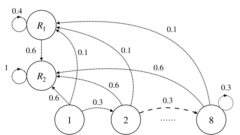
(a) Action repair.

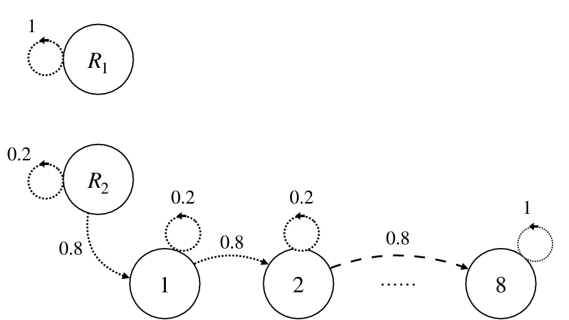
(b) Action wait.

Figure 9: Nominal transitions for the machine replacement instance.

21.1.3 Instance inspired by healthcare

We present in Figure 10 the nominal transitions for this instance, in the case of $8$ health conditions states. This goal is to minimize the mortality rate of the patient while reducing the invasiveness of the drug dosage (low, medium or high) prescribed at each state. Similarly, as for the machine replacement instance, the instances for a larger number of states are constructed by adding some health condition states for the patient.

States.

There are $S$ states. The first $S-1$ states represent the health conditions of the patient, with $S-1$ being the worst condition before the mortality absorbing state $m$.

Actions.

The action set is $\mathcal{A}=\{\sf low,medium,high\}$, representing the drug dosage at each state.

Transitions.

The transitions are represented in Figure 10. They capture the fact that the patient is more likely to recover (i.e., transitioning early states) under the high-intensity treatment (Figure 10(c)) than under the low-intensity treatment (Figure 10(a)).

Rewards.

The rewards penalize using an intense treatment plan for the patient. In a health condition state $s\in\{1,...,S-1\}$, the reward is $10$ for choosing action low, $8$ for choosing action medium, and $6$ for choosing action high.

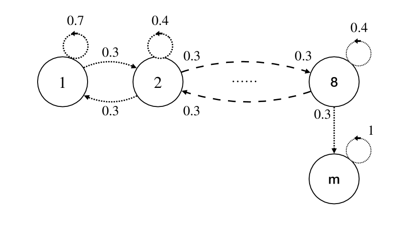
(a) Action low.

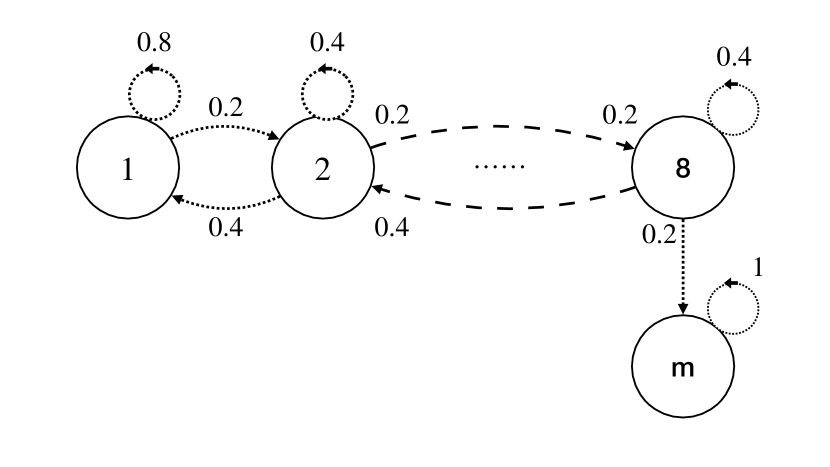
(b) Action medium.

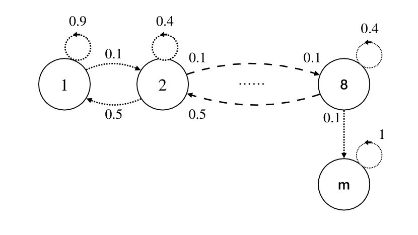
(c) Action high.

Figure 10: Nominal transitions for the MDP instance inspired from healthcare.

21.2 Uncertainty sets and practical implementation

21.2.1 The case of special transitions.

There are absorbing states in the three instances used in our experiments. In non-absorbing states, some transition probabilities toward other states may be $0$, e.g., in the machine replacement instance, transitioning from one of the operative states to a repair state without repairing. Since these transitions may reflect real physical constraints, in the implementation of our algorithms we ensure that the resulting worst-case transition probabilities have the same support as the nominal transitions, e.g., that transitions that are impossible for the nominal transition probabilities remain impossible for the worst-case transitions, and that absorbing states for the nominal transitions remain absorbing for the worst-case transitions.

21.2.2 Uncertainty based on ellipsoids.

The ellipsoidal uncertainty set is $\mathcal{U}_{sa}^{\sf\ell_{2}}=\{\bm{p}\in\Delta(\mathcal{S})\;|\;\|\bm{p}-\bm{p}_{{\sf nom},sa}\|_{2}\leq\alpha\},\forall\;(s,a)\in\mathcal{S}\times\mathcal{A}$ where $\alpha>0$ is a scalar. We use a radius $\alpha=0.05$. To evaluate the Bellman operator $T$ at a vector $\bm{v}\in\mathbb{R}^{\mathcal{S}}$, we would need to solve the following convex program: $\min_{\bm{p}\in\mathcal{U}_{sa}}\bm{p}^{\top}\bm{v}^{\prime}$ with $\bm{v}^{\prime}=(\bm{r}_{sa}+\gamma\bm{v})$, which may considerably increase the computation time of our algorithms, where the Bellman operator needs to be evaluated at every iteration. To ensure a fast implementation, we make the following assumption, building up on the analysis in Grand-Clément and Kroer [2021, 2023].

Assumption 21.1

The radius $\alpha>0$ is such that, for any $(s,a)\in\mathcal{S}\times\mathcal{A}$, we have

$$\{\bm{p}\in\mathbb{R}^{n}\;|\;\bm{p}^{\top}\bm{e}=1\}\cap\{\bm{p}\in\mathbb{R}^{\mathcal{S}}\;|\|\bm{p}-\bm{p}_{sa}\|_{2}\leq\alpha\}\subset\Delta(\mathcal{S}).$$

Assumption 21.1 has the simple interpretation that the orthogonal projection of the $\ell_{2}$-ball $\{\bm{p}\in\mathbb{R}^{\mathcal{S}}\;|\|\bm{p}-\bm{p}_{sa}\|_{2}\leq\alpha\}$ onto the hyperplane $\{\bm{p}\in\mathbb{R}^{n}\;|\;\bm{p}^{\top}\bm{e}=1\}$ is entirely contained into the simplex. Note that from Section 21.2.1, we only consider that transition probabilities in $(0,1)$ are uncertain so that Assumption 21.1 holds for a radius $\alpha$ small enough. Under this assumption, we can write $\mathcal{U}_{sa}^{\ell_{2}}$ as $\mathcal{U}_{sa}^{\ell_{2}}=\bm{p}_{{\sf nom},sa}+\alpha\tilde{B}$ with $\tilde{B}=\{\bm{z}\in\mathbb{R}^{\mathcal{S}}\;|\;\bm{z}^{\top}\bm{e}=0,\|\bm{z}\|_{2}\leq 1\}.$ Let us now write $\bm{u}_{1},...,\bm{u}_{|\mathcal{S}|-1}\in\mathbb{R}^{|\mathcal{S}|}$ an orthonormal basis of $\{\bm{p}\in\mathbb{R}^{n}\;|\;\bm{p}^{\top}\bm{e}=0\}$, e.g. the one given in closed-form in Egozcue et al. [2003]. Then writing $\bm{U}=\left(\bm{u}_{1},...,\bm{u}_{|\mathcal{S}|-1}\right)\in\mathbb{R}^{|\mathcal{S}|\times(|\mathcal{S}|-1)}$, and noting by definition $\bm{U}^{\top}\bm{U}=\bm{I}_{|\mathcal{S}|-1}$, we have

$$\tilde{B}=\{\bm{z}\in\mathbb{R}^{\mathcal{S}}\;|\;\bm{z}^{\top}\bm{e}=0,\|\bm{z}\|_{2}\leq 1\}=\{\bm{Uy}\;|\;\bm{y}\in\mathbb{R}^{|\mathcal{S}|-1},\|\bm{Uy}\|_{2}\leq 1\}=\{\bm{Uy}\;|\;\bm{y}\in\mathbb{R}^{|\mathcal{S}|-1},\|\bm{y}\|_{2}\leq 1\}$$

where the last equality follows from $\bm{U}$ being an orthonormal basis of $\{\bm{p}\in\mathbb{R}^{n}\;|\;\bm{p}^{\top}\bm{e}=0\}$. This shows that under Assumption 21.1, we have the following closed-form update: for $\bm{v}\in\mathbb{R}^{\mathcal{S}}$,

$$\min_{\bm{p}\in\mathcal{U}_{sa}}\bm{p}^{\top}\bm{v}=\bm{p}_{{\sf nom},sa}^{\top}\bm{v}+\alpha\min_{\bm{y}\in\mathbb{R}^{|\mathcal{S}|-1},\|\bm{y}\|_{2}\leq 1}\left(\bm{Uy}\right)^{\top}\bm{v}=\bm{p}_{{\sf nom},sa}^{\top}\bm{v}-\alpha\|\bm{U}^{\top}\bm{v}\|_{2}.$$

Overall, our analysis shows that in the case of ellipsoidal uncertainty as in $\mathcal{U}^{\sf\ell_{2}}$ and under Assumption 21.1, we can efficiently evaluate $T_{s}(\bm{v})$ as $T_{s}(\bm{v})=\max_{a\in\mathcal{A}}\bm{p}_{{\sf nom},sa}^{\top}\left(\bm{r}_{sa}+\gamma\bm{v}\right)-\alpha\|\bm{U}^{\top}\left(\bm{r}_{sa}+\gamma\bm{v}\right)\|_{2},\forall\;s\in\mathcal{S}.$

21.2.3 Uncertainty based on box inequalities.

We also consider the following uncertainty set: $\mathcal{U}_{sa}^{\sf box}=\{\bm{p}\in\Delta(\mathcal{S})\;|\;\bm{p}_{sa}^{\sf low}\leq\bm{p}\leq\bm{p}_{sa}^{\sf up}\},\forall\;(s,a)\in\mathcal{S}\times\mathcal{A}$ with $\bm{p}_{sa}^{\sf low},\bm{p}_{sa}^{\sf up}\in[0,1]^{\mathcal{S}}$ two vectors such that $\bm{p}_{sa}^{\sf low}\leq\bm{p}_{{\sf nom},sa}\leq\bm{p}_{sa}^{\sf up}.$ We build $\bm{p}_{sa}^{\sf low},\bm{p}_{sa}^{\sf up}$ as follows. We choose two scalars $\theta_{\sf up},\theta_{\sf low}$. The vector $\bm{p}_{sa}^{\sf low}$ is then the convex combination of $\bm{p}_{{\sf nom},sa}$ and $\bm{0}$ with coefficient $\theta_{\sf low}$, and $\bm{p}_{sa}^{\sf up}$ is then the convex combination of $\bm{p}_{{\sf nom},sa}$ and $\bm{e}$ with coefficient $\theta_{\sf up}$: $\bm{p}^{\sf up}_{sa}=(1-\theta_{\sf up})\bm{p}_{{\sf nom},sa}+\theta_{\sf up}\bm{e},\bm{p}^{\sf low}_{sa}=(1-\theta_{\sf low})\bm{p}_{{\sf nom},sa}.$ In our numerical experiment we use $\theta_{\sf up}=\theta_{\sf low}=0.05.$ Note that to evaluate the Bellman operator $T$ at a vector $\bm{v}\in\mathbb{R}^{\mathcal{S}}$, we only need to sort the component of $\bm{v}$ in increasing order and then use the closed-form expression from the method described in proposition 3 in Goh et al. [2018].

21.3 Implementation of Algorithm 1

In Algorithm 1, at every iteration $t$ we compute $\bm{v}^{\star,\mathcal{U}}_{\gamma_{t}}$ by implementing two-player Strategy Iteration [Hansen et al., 2013], as described in Algorithm 4.

Algorithm 4 Two-player Strategy Iteration for sa-rectangular robust MDPs

Input: Initial policy $\pi^{\sf start}\in\Pi_{\sf SD}$

Initialize $\pi^{0}=\pi^{\sf start}\in\Pi_{\sf SD}$.

for $t\in\mathbb{N}$ do

     Policy Evaluation: $\bm{v}^{t}=\bm{v}^{\pi^{t},\mathcal{U}}_{\gamma}$

     Policy Improvement: choose $\pi^{t+1}\in\Pi_{\sf SD}$ such that

$$\pi^{t+1}(s)\in\arg\max_{a\in\mathcal{A}}\min_{\bm{p}_{sa}\in\mathcal{U}_{sa}}\bm{p}_{sa}^{\top}\left(\bm{r}_{sa}+\gamma\bm{v}^{t}\right),\forall\;s\in\mathcal{S},$$

with $\pi^{t+1}(s)=\pi^{t}(s)$ if possible.

     stop if $\pi^{t+1}=\pi^{t}$.

end for

Recall that in Algorithm 1, we compute the optimal discounted policies for an increasing sequence of discount factors. Therefore, we warm-start Algorithm 4 at the next iteration with the policy computed at the previous iteration. This considerably reduces the computation time, for two reasons:

1. The discount factors $\gamma_{t}$ at iteration $t$ and $\gamma_{t+1}$ at iteration $t+1$ are close so that we can expect the optimal policies at iteration $t$ and iteration $t+1$ to be close;

2. Since $\mathcal{U}^{\sf box}$ and $\mathcal{U}^{\ell_{2}}$ are definable sets, Blackwell optimal policies exist. A Blackwell discount factor also exists, and for $\gamma$ large enough, the set of optimal stationary deterministic policies does not change.

In Algorithm 4, we compute the robust value function of $\pi^{t}$ at every iteration $t$. We do so by implementing the one-player version of Policy Iteration for the adversarial MDP [Ho et al., 2021, Goh et al., 2018]) as in Algorithm 5.

Algorithm 5 Policy Iteration for the Adversarial MDPs

Input: Stationary policy $\pi\in\Pi_{\sf S}$, initial transition probabilities $\bm{P}^{\sf start}\in\mathcal{U}$

Initialize $\bm{P}^{0}=\bm{P}^{\sf start}$.

for $t\in\mathbb{N}$ do

     Adversarial Policy Evaluation: $\bm{v}^{t}=\bm{v}^{\pi,\bm{P}^{t}}_{\gamma}$

     Adversarial Policy Improvement: choose $\bm{P}^{t+1}\in\mathcal{U}$ such that

$$\bm{p}^{t+1}_{sa}\in\arg\min_{\bm{p}_{sa}\in\mathcal{U}_{sa}}\bm{p}_{sa}^{\top}\left(\bm{r}_{sa}+\gamma\bm{v}^{t}\right),\forall\;(s,a)\in\mathcal{S}\times\mathcal{A}$$

with $\bm{P}^{t+1}_{sa}=\bm{P}^{t}_{sa}$ if possible.

     stop if $\bm{p}^{t+1}=\bm{p}^{t}$.

end for

We also use warm-starting to accelerate the practical performance of Algorithm 5.

References

- Akian et al. [2019] Marianne Akian, Stéphane Gaubert, Julien Grand-Clément, and Jérémie Guillaud. The operator approach to entropy games. Theory of Computing Systems, 63(5):1089–1130, 2019.
- Andersson and Miltersen [2009] Daniel Andersson and Peter Bro Miltersen. The complexity of solving stochastic games on graphs. In International Symposium on Algorithms and Computation, pages 112–121. Springer, 2009.
- Ashok et al. [2017] Pranav Ashok, Krishnendu Chatterjee, Przemysław Daca, Jan Křetínskỳ, and Tobias Meggendorfer. Value iteration for long-run average reward in Markov decision processes. In Computer Aided Verification: 29th International Conference, CAV 2017, Heidelberg, Germany, July 24-28, 2017, Proceedings, Part I, pages 201–221. Springer, 2017.
- Bäuerle and Rieder [2011] Nicole Bäuerle and Ulrich Rieder. Markov decision processes with applications to finance. Springer Science & Business Media, 2011.
- Baxter and Bartlett [2001] Jonathan Baxter and Peter L Bartlett. Infinite-horizon policy-gradient estimation. journal of artificial intelligence research, 15:319–350, 2001.
- Behzadian et al. [2021] Bahram Behzadian, Marek Petrik, and Chin Pang Ho. Fast algorithms for constrained s-rectangular robust MDPs. Advances in Neural Information Processing Systems, 34:25982–25992, 2021.
- Bennett and Hauser [2013] Casey C Bennett and Kris Hauser. Artificial intelligence framework for simulating clinical decision-making: A Markov decision process approach. Artificial intelligence in medicine, 57(1):9–19, 2013.
- Bierth [1987] K-J Bierth. An expected average reward criterion. Stochastic processes and their applications, 26:123–140, 1987.
- Blackwell and Ferguson [1968] David Blackwell and Tom S Ferguson. The big match. The Annals of Mathematical Statistics, 39(1):159–163, 1968.
- Bolte et al. [2015] Jérôme Bolte, Stéphane Gaubert, and Guillaume Vigeral. Definable zero-sum stochastic games. Mathematics of Operations Research, 40(1):171–191, 2015.
- Brockman et al. [2016] Greg Brockman, Vicki Cheung, Ludwig Pettersson, Jonas Schneider, John Schulman, Jie Tang, and Wojciech Zaremba. Openai gym. arXiv preprint arXiv:1606.01540, 2016.
- Chae et al. [2022] Jongseong Chae, Seungyul Han, Whiyoung Jung, Myungsik Cho, Sungho Choi, and Youngchul Sung. Robust imitation learning against variations in environment dynamics. In International Conference on Machine Learning, pages 2828–2852. PMLR, 2022.
- Choudary and Niculescu [2014] Alla Dita Raza Choudary and Constantin P Niculescu. Real analysis on intervals. Springer, 2014.
- Condon [1992] Anne Condon. The complexity of stochastic games. Information and Computation, 96(2):203–224, 1992.
- Cordwell et al. [2015] Steven Cordwell, Yasser Gonzalez, and Theja Tulabandhula. Markov Decision Process (MDP) toolbox for python. https://github.com/sawcordwell/pymdptoolbox, 2015.
- Coste [2000] Michel Coste. An introduction to o-minimal geometry. Istituti editoriali e poligrafici internazionali Pisa, 2000.
- Delage and Mannor [2010] Erick Delage and Shie Mannor. Percentile optimization for Markov decision processes with parameter uncertainty. Operations research, 58(1):203–213, 2010.
- Deng et al. [2016] Yue Deng, Feng Bao, Youyong Kong, Zhiquan Ren, and Qionghai Dai. Deep direct reinforcement learning for financial signal representation and trading. IEEE transactions on neural networks and learning systems, 28(3):653–664, 2016.
- Dewanto et al. [2020] Vektor Dewanto, George Dunn, Ali Eshragh, Marcus Gallagher, and Fred Roosta. Average-reward model-free reinforcement learning: a systematic review and literature mapping. arXiv preprint arXiv:2010.08920, 2020.
- Egozcue et al. [2003] Juan José Egozcue, Vera Pawlowsky-Glahn, Glòria Mateu-Figueras, and Carles Barcelo-Vidal. Isometric logratio transformations for compositional data analysis. Mathematical geology, 35(3):279–300, 2003.
- Feinberg and Shwartz [2012] Eugene A Feinberg and Adam Shwartz. Handbook of Markov decision processes: methods and applications, volume 40. Springer Science & Business Media, 2012.
- Filar and Vrieze [2012] Jerzy Filar and Koos Vrieze. Competitive Markov decision processes. Springer Science & Business Media, 2012.
- Gillette [1957] Dean Gillette. Stochastic games with zero stop probabilities. Contributions to the Theory of Games, 3:179–187, 1957.
- Gimbert and Kelmendi [2023] Hugo Gimbert and Edon Kelmendi. Submixing and shift-invariant stochastic games. International Journal of Game Theory, pages 1–36, 2023.
- Givan et al. [1997] Robert Givan, Sonia Leach, and Thomas Dean. Bounded parameter Markov decision processes. In European Conference on Planning, pages 234–246. Springer, 1997.
- Goh et al. [2018] Joel Goh, Mohsen Bayati, Stefanos A Zenios, Sundeep Singh, and David Moore. Data uncertainty in Markov chains: Application to cost-effectiveness analyses of medical innovations. Operations Research, 66(3):697–715, 2018.
- Goyal and Grand-Clément [2022] Vineet Goyal and Julien Grand-Clément. Robust Markov decision processes: Beyond rectangularity. Mathematics of Operations Research, 2022.
- Grand-Clément and Kroer [2021] Julien Grand-Clément and Christian Kroer. Conic blackwell algorithm: Parameter-free convex-concave saddle-point solving. Advances in Neural Information Processing Systems, 34:9587–9599, 2021.
- Grand-Clement and Kroer [2021] Julien Grand-Clement and Christian Kroer. First-order methods for wasserstein distributionally robust MDP. In International Conference on Machine Learning, pages 2010–2019. PMLR, 2021.
- Grand-Clément and Kroer [2023] Julien Grand-Clément and Christian Kroer. Solving optimization problems with blackwell approachability. Mathematics of Operations Research, 2023.
- Grand-Clément and Petrik [2022] Julien Grand-Clément and Marek Petrik. On the convex formulations of robust Markov decision processes. arXiv preprint arXiv:2209.10187, 2022.
- Grand-Clément and Petrik [2023] Julien Grand-Clément and Marek Petrik. Reducing blackwell and average optimality to discounted MDPs via the blackwell discount factor. arXiv preprint arXiv:2302.00036, 2023.
- Grand-Clément et al. [2023] Julien Grand-Clément, Carri W Chan, Vineet Goyal, and Gabriel Escobar. Robustness of proactive intensive care unit transfer policies. Operations Research, 71(5):1653–1688, 2023.
- Hansen et al. [2013] Thomas Dueholm Hansen, Peter Bro Miltersen, and Uri Zwick. Strategy iteration is strongly polynomial for 2-player turn-based stochastic games with a constant discount factor. Journal of the ACM (JACM), 60(1):1–16, 2013.
- Ho et al. [2021] Chin Pang Ho, Marek Petrik, and Wolfram Wiesemann. Partial policy iteration for l1-robust Markov decision processes. The Journal of Machine Learning Research, 22(1):12612–12657, 2021.
- Ho et al. [2022] Chin Pang Ho, Marek Petrik, and Wolfram Wiesemann. Robust phi-divergence MDPs. arXiv preprint arXiv:2205.14202, 2022.
- Iyengar [2005] G. Iyengar. Robust dynamic programming. Mathematics of Operations Research, 30(2):257–280, 2005.
- Kumar et al. [2023] Navdeep Kumar, Esther Derman, Matthieu Geist, Kfir Levy, and Shie Mannor. Policy gradient for s-rectangular robust Markov decision processes. arXiv preprint arXiv:2301.13589, 2023.
- Laraki and Sorin [2015] Rida Laraki and Sylvain Sorin. Advances in zero-sum dynamic games. In Handbook of game theory with economic applications, volume 4, pages 27–93. Elsevier, 2015.
- Le Tallec [2007] Yann Le Tallec. Robust, risk-sensitive, and data-driven control of Markov decision processes. PhD thesis, Massachusetts Institute of Technology, 2007.
- Leizarowitz [2003] Arie Leizarowitz. An algorithm to identify and compute average optimal policies in multichain markov decision processes. Mathematics of Operations Research, 28(3):553–586, 2003.
- Li et al. [2023] Mengmeng Li, Tobias Sutter, and Daniel Kuhn. Policy gradient algorithms for robust MDPs with non-rectangular uncertainty sets. arXiv preprint arXiv:2305.19004, 2023.
- Li et al. [2022] Yan Li, Tuo Zhao, and Guanghui Lan. First-order policy optimization for robust Markov decision process. arXiv preprint arXiv:2209.10579, 2022.
- Mannor et al. [2016] S. Mannor, O. Mebel, and H. Xu. Robust MDPs with k-rectangular uncertainty. Mathematics of Operations Research, 41(4):1484–1509, 2016.
- Mertens et al. [2015] Jean-François Mertens, Sylvain Sorin, and Shmuel Zamir. Repeated games, volume 55. Cambridge University Press, 2015.
- Mnih et al. [2013] Volodymyr Mnih, Koray Kavukcuoglu, David Silver, Alex Graves, Ioannis Antonoglou, Daan Wierstra, and Martin Riedmiller. Playing atari with deep reinforcement learning. arXiv preprint arXiv:1312.5602, 2013.
- Neyman et al. [2003] Abraham Neyman, Sylvain Sorin, and S Sorin. Stochastic games and applications, volume 570. Springer Science & Business Media, 2003.
- Nilim and Ghaoui [2005] A. Nilim and L. El Ghaoui. Robust control of Markov decision processes with uncertain transition probabilities. Operations Research, 53(5):780–798, 2005.
- Panaganti and Kalathil [2022] Kishan Panaganti and Dileep Kalathil. Sample complexity of robust reinforcement learning with a generative model. In International Conference on Artificial Intelligence and Statistics, pages 9582–9602. PMLR, 2022.
- Possingham and Tuck [1997] Hugh Possingham and G Tuck. Application of stochastic dynamic programming to optimal fire management of a spatially structured threatened species. In Proceedings International Congress on Modelling and Simulation, MODSIM, pages 813–817, 1997.
- Puterman [2014] Martin L Puterman. Markov decision processes: discrete stochastic dynamic programming. John Wiley & Sons, 2014.
- Renault [2019] Jérôme Renault. A tutorial on zero-sum stochastic games. arXiv preprint arXiv:1905.06577, 2019.
- Satia and Lave [1973] J.K. Satia and R.L. Lave. Markov decision processes with uncertain transition probabilities. Operations Research, 21(3):728–740, 1973.
- Shapley [1953] Lloyd S Shapley. Stochastic games. Proceedings of the national academy of sciences, 39(10):1095–1100, 1953.
- Sorin [2002] Sylvain Sorin. A first course on zero-sum repeated games, volume 37. Springer Science & Business Media, 2002.
- Steimle and Denton [2017] Lauren N Steimle and Brian T Denton. Markov decision processes for screening and treatment of chronic diseases. Markov Decision Processes in Practice, pages 189–222, 2017.
- Sutton and Barto [2018] Richard S Sutton and Andrew G Barto. Reinforcement learning: An introduction. MIT press, 2018.
- Tewari and Bartlett [2007] Ambuj Tewari and Peter L Bartlett. Bounded parameter Markov decision processes with average reward criterion. In International Conference on Computational Learning Theory, pages 263–277. Springer, 2007.
- Van Den Dries [1998] Lou Van Den Dries. O-minimal structures and real analytic geometry. Current developments in mathematics, 1998(1):105–152, 1998.
- Van den Dries and Miller [1996] Lou Van den Dries and Chris Miller. Geometric categories and o-minimal structures. 1996.
- Viano et al. [2021] Luca Viano, Yu-Ting Huang, Parameswaran Kamalaruban, Adrian Weller, and Volkan Cevher. Robust inverse reinforcement learning under transition dynamics mismatch. Advances in Neural Information Processing Systems, 34:25917–25931, 2021.
- Wang et al. [2022] Qiuhao Wang, Chin Pang Ho, and Marek Petrik. On the convergence of policy gradient in robust MDPs. arXiv preprint arXiv:2212.10439, 2022.
- Wang et al. [2023] Yue Wang, Alvaro Velasquez, George Atia, Ashley Prater-Bennette, and Shaofeng Zou. Robust average-reward Markov decision processes. arXiv preprint arXiv:2301.00858, 2023.
- Wiesemann et al. [2013] Wolfram Wiesemann, Daniel Kuhn, and Berç Rustem. Robust Markov decision processes. Mathematics of Operations Research, 38(1):153–183, 2013.
- Xu and Mannor [2010] Huan Xu and Shie Mannor. Distributionally robust Markov decision processes. Advances in Neural Information Processing Systems, 23, 2010.
- Zhang et al. [2017] Yuanhui Zhang, L Steimle, and BT Denton. Robust Markov decision processes for medical treatment decisions. Optimization online, 2017.
- Zwick and Paterson [1996] Uri Zwick and Mike Paterson. The complexity of mean payoff games on graphs. Theoretical Computer Science, 158(1-2):343–359, 1996.