Time-Domain Operational Metrics for Real-time Resilience Assessment in DC Microgrids

Abstract

Resilience is emerging as an evolving notion, reflecting a system’s ability to endure and adapt to sudden and catastrophic changes and disruptions. This paper spotlights the significance of the quantitative resilience indices of medium-voltage DC (MVDC) distribution technology in marine vessels, notably naval ships. Given the intricate electrical requirements of modern naval ships, the need for a robust power supply underlines the imperative of resilient DC microgrids. Addressing this, our study introduces a novel quantitative metric for operational resilience of DC microgrids based on the measured voltage of main DC bus. This metric not only fuses real-time tracking, compatibility, and computational efficiency, but also adeptly monitors multiple event phases based on time-domain analysis of dc bus voltage dynamics. The intricacies of the dc bus voltage, including overshoots and undershoots, are meticulously accounted for in the algorithm design. With respect to existing research that typically focuses on offline resilience assessments, the proposed index provides valuable real-time information for microgrid operators and identifies whether microgrid resilience is deteriorating over time.

I Introduction

Currently, resilience is seen as a evolving idea in power systems, characterized as “a measure of the persistence of systems and of their ability to absorb change and disturbances and recover from failures”. Broadly, “resilience is defined as the ability of equipment, networks, and systems to predict, absorb, and quickly recover from catastrophic events” [1].

Medium-voltage DC (MVDC) distribution technology, used in various infrastructures, offers many benefits, especially in marine vessels such as naval ships. These benefits include easy integration of renewable energy, improved fuel efficiency, and better power quality than AC systems [2]. Given the significant electrical needs of naval ships, which encompass advanced weaponry, navigation systems, and communication apparatus, MVDC shipboard microgrids are considered in this paper. Due to the significance of mission operation for navy ships, resilience of shipboard microgrids becomes imperative.

An integral preliminary action to do so, would be to formulate a method to quantitatively assess the operational health and efficacy of the navy’s electrical infrastructure on ships [3]. Consequently, it is important that the resilience quantification index possess attributes of compatibility; it should draw insights from historical events and learn from past events, be real-time and online, be applicable at the system level, and be computationally efficient [4].

Table I: Qualitative comparison between the state-Of-the-art metrics.

Ref.	Metric	Computationally efficient	Scalability	Real-time	System level
[5]	$\Re=\xi(LOLP,EDNS,Y,\Psi,\Lambda)$	$\times$	$\checkmark$	$\times$	Transmission
[6]	$\begin{aligned} &\mathfrak{R}=\int_{t}S(t)dt\\ &\mathfrak{R}=\sum n\\ &\mathfrak{R}=\frac{\sum_{i=1}^{N}t_{up,i}}{\sum_{i=1}^{N}\left(t_{up,i}+t_{\text{down },i}\right)}\end{aligned}$	$\times$	$\times$	$\times$	Distribution
[7]	$\vec{\Re}=\left[F_{c},D_{G},l_{G},C_{B},C_{n},\Lambda_{2}\right]$	$\checkmark$	$\times$	$\times$	Distribution
[8]	$\mathfrak{R}=(\Phi\Lambda E\Pi)$	$\checkmark$	$\times$	$\times$	Distribution
[9]	$\Re=FI+(1-REI)+MVI+LLI$	$\times$	$\times$	$\checkmark$	Microgrid
[10]	$\mathfrak{R}=\frac{1}{NT}\sum_{h=1}^{NT}\sum_{t=1}^{N}\sum_{t=h+1}^{h+H}\Delta t.LS$	$\times$	$\times$	$\times$	Microgrid
[11]	$\Re=\xi(LOLP,EDNS,F,G)$	$\times$	$\times$	$\checkmark$	Microgrid
Proposed	$\Re=\xi(R_{V},V_{VI},V_{DI},V_{REI})$	$\checkmark$	$\checkmark$	$\checkmark$	Microgrid

Several studies have focused on developing resilience assessment tools for microgrids and power systems in general [5, 6, 7, 8, 9, 10, 11]. In Table I, a comprehensive comparison of various metrics is presented, which compares the application level (i.e., transmission, distribution, and microgrid) and real-time/offline assessment features of existing resilience metrics. As it can be observed, not many existing studies focused on real-time resilience assessment tools for microgrids nor offer a computationally effective approach that is also scalable and can be accommodated for various microgrid designs. To the best of our knowledge, there exists no previous research that presents a set of metrics within the context of real-time operational resilience assessment for DC microgrids that are capable of quantifying various event phases, ensuring computational efficiency, exhibiting compatibility, and offering real-time tracking. To address this gap, we propose a voltage resilience metric in real-time that can be tracked using available measurement and is applicable to various DC microgrid designs. It offers a harmonious blend of compatibility with various microgrid designs, computational efficiency, and real-time applicability, establishing it as a noteworthy breakthrough. Additionally, compared with existing real-time indexes in [9, 11, 12], the proposed metric distinguishes itself by providing real-time tracking for various phases of an event in a microgrid, such as the degradation phase, restoration phase, and the degree of degradation. Specifically, the paper enumerates its distinguished contributions as follows:

1. Proposing a distinctive resilience metric tailored for DC microgrids that offers real-time tracking, compatibility, and computational efficiency, filling an evident gap in existing research.

2. The proposed metric is further enhanced to provide real-time monitoring across varied event phases, including the degradation phase, restoration phase, and the degree of degradation, all contingent on the dc bus voltage dynamics within Navy shipboard microgrids.

3. An algorithm is developed to utilize the proposed resilience index and assess DC microgrid’s resilience during events via DC voltage overshoots, undershoots, and fluctuations.

The rest of the paper is structured as follows. Dynamic model of the system is explained in Section II and the proposed resilience indices are described in Section III. Section IV validates of the proposed metrics through several case studies and conclusions are drawn in Section V.

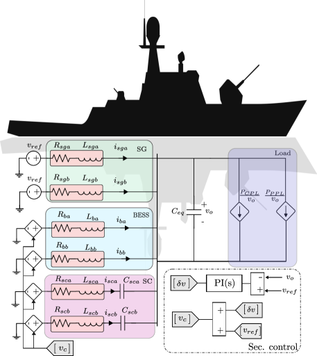
Figure 1: Closed-loop MVDC microgrid configuration for Navy shipboards.

II Methodology

II-A Model Description

Fig. 1, illustrates an equivalent circuit of a 6kV MVDC shipboard microgrid inspired from [13]. Within this microgrid, power sources operate with secondary control design. Synchronous generators (SGs) mainly contribute to the low-frequency loads,such as constant power loads $P_{CPL}$. To address rapidly varying loads such as pulsed power loads (PPLs) $P_{PPL}$, two battery energy storage units (BESS) and supercapacitors (SCs) are designed and to reduce the current stress on BESSs. In this system, subsequent to any event or load changes, the droop controller determines voltage shifts for the main bus. This can be mathematically written by:

$$v_{t} ={v_{o_{DC}}}-R_{\text{eq}}i_{\text{load}}$$ (1)

$$={v_{o_{DC}}}-\left(R_{sga}||R_{sgb}||R_{ba}||R_{bb}\right)\frac{P_{\text{load}}}{v_{t}}$$ (2)

where ${v_{o_{DC}}}$ stands for the reference voltage which is 6KV in this system. Also, $v_{t}$ is the MVDC real-time voltage measurement across the DC link capacitor $C_{\text{eq}}$, and $R_{eq}$ denotes the equivalent resistive droop gain of the system for the conventional generators and BESSs. Comprehensive information regarding the droop control design for the ship can be found in [14]. The total load power is also represented by $P_{\text{load}}$. To restore voltage fluctuations arising from the droop controller after events, the secondary voltage control has been utilized to stabilize the voltage trajectory, as illustrated in Fig. 1.

II-B Reduced order model of MVDC shipboard microgrids

The open loop differential equations of the system in Fig. 1 can be formulated as follows [13]:

$$C_{\text{eq}}\dot{v_{t}} =\frac{}{}\sum_{i\in\mathcal{N}_{SG}}(i_{\text{SG}i})+\sum_{i\in\mathcal{N}_{B}}(i_{\text{B}i})+\sum_{i\in\mathcal{N}_{SC}}(i_{\text{SC}i})$$

$$-\frac{P_{\text{CPL}}}{v_{t}}-\frac{P_{\text{PPL}}}{v_{t}}$$ (3a)

$$L_{i}\dot{i}_{i} ={v_{o_{DC}}}-R_{i}i_{i}-v_{t}+\delta v_{i}\quad\forall i\in\{\mathcal{N}_{SG},\mathcal{N}_{B}\}$$ (3b)

$$L_{i}\dot{i}_{i} ={v_{o_{DC}}}-R_{i}i_{i}-v_{SCi}-v_{t}\quad\forall i\in\mathcal{N}_{SC}$$ (3c)

$$C_{i}\dot{v}_{Ci} =i_{i}\quad\forall i\in\mathcal{N}_{SC}$$ (3d)

where $L_{i}$ is the equivalent inductance of the $i$-th generation unit, $v_{t}$ denotes the output voltage in real-time, $i_{i}$ is the current of the $k$-th generation unit, and $R_{i}$ is the resistive droop gains for the conventional generators and BESSs, respectively. Centralized $\delta v$ using a PI controller is used, which guarantees voltage restoration (Fig. 1).

In Fig. 2, the voltage restoration of the main bus after a sudden load change is depicted. A comparative analysis of this dynamic behavior against a detailed simulation-based model is also presented. The results clearly illustrate that the dynamic behavior of the reduced-order closed-loop model closely aligns with the detailed model.

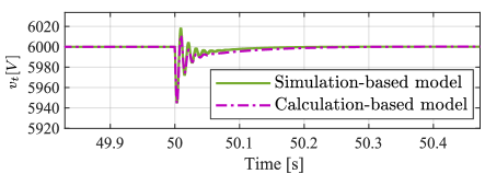
Figure 2: Verifying the calculation-based model under sudden load change.

III Proposed Time-domain Voltage Resiliency Index

When an extreme event impacts the power system, the system’s attributes might deviate from their normal state. This time-dependent fluctuation of a system attribute in response to such an event is termed as the system performance. Power system performance can be assessed using various metrics of performance (MoP), including:

• 1. The percentage of total or critical loads.

• 2. The number of supplied critical loads.

• 3. The count of survived or failed loads.

• 4. Technical metrics, i.e., voltage and frequency [12].

In this study, we underscore the significance of ranking MoPs based on the system’s operational strategies and goals in real-time. As such, our primary emphasis is on appraising system’s resilience and technical performance via voltage indices.

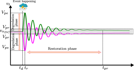
Figure 3: Microgrid voltage performance curve during an event.

Fig. 3 depicts the voltage response of a DC microgrid during extreme events, such as sudden load changes or generator failures in the MG. Upon the event’s onset at $t_{d}$, the system’s performance experiences a noticeable degradation to $V_{pe}$, causing the voltage to deviate from its reference value $v_{o_{DC}}$. This deviation, which may manifest as overshoot or undershoot, reflects the system’s transient response to such disturbances. As time progresses to $t_{r}$, the system begins its restoration phase, facilitated by the MG controllers. By time $t_{pr}$, the system voltage has been fully restored to its reference or desired value. Hence, the proposed set of resiliency metrics, representing various phases of the system during an event is formulated as:

$$\Re=\xi(R_{V},V_{VI},V_{DI},V_{REI})$$ (4)

To evaluate the MG’s ability to draw insights from past events, and show its degradation over time, we introduce the index $R_{V}$. This metric quantifies the MG’s voltage compatibility and its capacity to retain memory from prior events. More importantly, it manifests the MG’s inherent capability to learn and remember past voltage perturbations. Therefore, mathematically, it can be formulated as:

$$R_{V}(t)=\int\left[{v_{o_{DC}}}-v_{t}(t)\right]dt$$ (5)

This equation captures the cumulative discrepancy between the reference voltage ${v_{o_{DC}}}$ and the real-time voltage ${v_{t}(t)}$ from the disturbance’s inception to its termination. To calculate the corrosponding area, we used the trapezoidal rule.

Theorem III.1.

The trapezoidal rule estimates the integral of a function by approximating the area under its graph as trapezoids. For enhanced accuracy, one can partition the interval into smaller subintervals. Let $\left\{x_{k}\right\}$ be a partition of $[a,b]$ such that $a=x_{0}<\cdots<x_{N-1}<x_{N}=b$ and $\Delta x_{k}=x_{k}-x_{k-1}$ be the length of the $k$-th subinterval, then the composite trapezoidal rule for uniform subintervals of size $\Delta x$, is given by: For uniform subintervals of size $\Delta x$, the formula simplifies to:

$$\int_{a}^{b}f(x)dx\approx\frac{\Delta x}{2}\left[f\left(x_{0}\right)+2\sum_{k=1}^{N-1}f\left(x_{k}\right)+f\left(x_{N}\right)\right]$$ (6)

Remark.

To apply this method in a real-time application, we should update the value of b to correspond only to the next $x_{k}$ at each simulation step.

To evaluate the extent of voltage degradation, a vulnerability index ($V_{VI}$) is introduced as: $V_{VI}=k*\frac{{v_{o_{DC}}}-V_{pe}}{{v_{o_{DC}}}}$ where, $k$ is the scaling factor. Under normal MG operational conditions, $V_{VI}$ is 0 and under a complete degradation, it is 1.

While the index $V_{VI}$ offers an immediate insight into the system’s voltage performance after an event, it lacks information about the system’s temporal behavior. Addressing this limitation, a normalized degradation index $V_{DI}$ is proposed:

$$V_{DI}=k*\frac{\int_{t_{d}}^{t_{r}}({v_{o_{DC}}}-v_{t}(t))dt}{{v_{o_{DC}}}(t_{r}-t_{d})}$$ (7)

where in a system exhibiting strong real-time resilience, the metric is 0, whereas for a fragile system experiencing a total loss of functionality, $V_{DI}$ equals 1. Algorithm 1 details the detection procedure for $V_{pe}$, $t_{r}$, and $t_{d}$ used in the calculation of $V_{DI}$. The coefficient $k$ is utilized to influence the magnitude of the index, ensuring that the resultant value of the index is appropriately scaled or minimized. Algorithm 1 displays the implementation of the $V_{DI}$ index in this study.

Remark.

Upon the occurrence of a disturbance, the voltage signal may exhibit transient behaviors, notably voltage rise or drop. To accurately account for this dynamic response in the proposed ${V_{DI}}$ algorithm, it becomes imperative to detect the value of ${V_{pe}}$ using instantaneous voltage measurements.

Input: $\text{clock},v_{t},{v_{o_{DC}}}$

1 Initialize persistent variables:     $time,v_{m}(t),v_{m}(t-1),t_{d},t_{r},S_{total},$     $Denom,t1,\Delta t$

2if $time$ is empty then

3       $time\leftarrow 0$

4:Initialize other persistent variables similarly Execute Nominator calculations;

5 $\Delta v\leftarrow v_{t}-{v_{o_{DC}}}$;

6

7if $v_{t}<{v_{o_{DC}}}$ or $v_{t}>{v_{o_{DC}}}$ then

8       $\delta t\leftarrow\lvert time-clock\rvert$;

9       $time\leftarrow clock$;

10       $S1\leftarrow\lvert\Delta v\rvert\times\delta t$;

11       $S_{total}\leftarrow S_{total}+S1$;

12      

13      Execute Denominator calculations;

14       if $v_{t}<{v_{o_{DC}}}$ or $v_{t}>{v_{o_{DC}}}$ then

15             $t1\leftarrow t1+1$;

16             $t_{r}\leftarrow clock$;

17             if $t1<1.5$ then

18                   $t_{d}\leftarrow clock$;

19                  

20            $\Delta t\leftarrow\lvert t_{r}-t_{d}\rvert$;

21             $Denom\leftarrow{v_{o_{DC}}}\times\Delta t$;

22            

23      

24

25if $v_{m}(t)==0$ or ($v_{m}(t-1)<v_{m}(t)$ and $v_{t}<{v_{o_{DC}}}$) or ($v_{m}(t-1)>v_{m}(t)$ and $v_{t}>{v_{o_{DC}}}$) then

26       $t1,t_{r},t_{d},S_{total}\leftarrow 0$;

27      

28

29if $v_{m}(t)==0$ or ($v_{m}(t-1)<v_{m}(t)$ and $v_{t}<{v_{o_{DC}}}$) or $v_{m}(t-1)==v_{m}(t)$ or ($v_{m}(t-1)>v_{m}(t)$ and $v_{t}>{v_{o_{DC}}}$) then

30       $V_{DI}\leftarrow 0$;

31      

32else

33       $V_{DI}\leftarrow\frac{S_{total}}{Denom\times{v_{o_{DC}}}}$;

34      

35

36$v_{m}(t-1)\leftarrow v_{m}(t)$;

37 return $V_{DI}$;

38

Algorithm 1 $V_{DI}$ Calculation Algorithm

Starting from $t_{r}$, the system transitions into its restoration phase, swiftly recovering to an acceptable performance level denoted by $V_{pr}$ at $t_{pr}$. This rapid recovery is made possible by the network’s redundancy, particularly through the design of an effective secondary controller. To evaluate the efficiency of this restoration phase, we introduce the voltage restoration efficiency index, $V_{REI}$, defined in Equation (8) as:

$$V_{REI}=\frac{\int_{t_{r}}^{t_{pr}}(v_{t}(t)-V_{pe})dt}{({v_{o_{DC}}}-V_{pe})(t_{pr}-t_{r})}$$ (8)

For an MG that can fully restore its functionality, the metric returns a value of 1. Conversely, if the MG fails to recover, the metric is calculated to be 0. Furthermore, this metric signifies how fast the MG can bounce back from the particular event.

IV Simulation results

The proposed resiliency evaluation method is validated for the MVDC microgrid depicted in Fig. 1. The simulation is conducted in MATLAB/Simulink running on a PC with Intel Core i9-10900X 3.7GHz and 64GB RAM under Windows 10. The sampling time for the simulation is set to $50\leavevmode\nobreak\ \mu s$.

IV-A Case studies

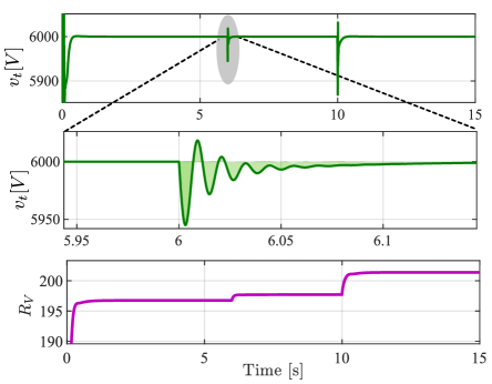
Figure 4: DC bus voltage and the $R_{V}$ index verification.

Table II: Different events and area analysis for $R_{V}$ index

	Time (s)	Area before event	Area after event	Added area
Event 1 ($P_{CPL}$ Load Change)	t = 6	196.7	197.7	1
Event 2 (Gen. failure)	t = 10	197.7	201.1	3.4

Fig. 4 depicts the DC bus voltage’s response to a sudden load change from 10 MW to 15 MW at $t=6s$ and a generator failure at $t=10s$. The ${R_{V}}$ index reflexes changes due to the computed area between the actual voltage deviation and the reference voltage according to Equation (5). The ${R_{V}}$ index visibly increases step by step in response to particular events and stops updating when the voltage stabilizes, offering insights into the system’s historical response to disturbances. This graphical evolution of the ${R_{V}}$ index, alongside Table II that categorizes the impact of such events by time and magnitude, provides a comprehensive analysis of the system’s resilience to disruptions.

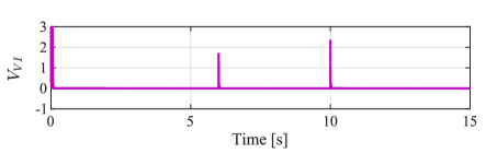
Figure 5: Voltage vulnerability index verification.

Fig. 5 depicts the verification of the voltage vulnerability index ($V_{VI}$), with $k=0.1$, under specified event scenarios. The $V_{VI}$ index elucidates how low resilience drops when the system encounters perturbations. The consistent monitoring of DC bus voltage and its subsequent deviations provide invaluable insights into the system’s vulnerability under these conditions.

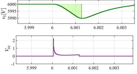
Figure 6: Voltage degradation index verification.

Fig. 6 presents the verification of the voltage degradation index within a narrowly defined time window. The upper subplot displays the behavior of the DC bus voltage, $V_{t}$, capturing a distinct perturbation around $t=6s$. The green area underscores the degradation area of this perturbation over time. Correspondingly, the lower subplot illustrates the ${V_{DI}}$ index’s response with $k=10e^{-5}$ to this voltage deviation. The ${V_{DI}}$ index, rendered in purple, signifies the normalized area of the degradation of voltage in real-time. As illustrated, this index not only pinpoints the onset of the event but also discerns the termination of the degradation phase. The precise time scale coupled with the conspicuous shift in the ${V_{DI}}$ index underscores the criticality of immediate monitoring for maintaining voltage stability.

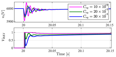
Figure 7: Impact of $C_{eq}$ on voltage transient behavior of MVDC and the voltage restoration efficiency index verification.

In the MVDC system, the $C_{eq}$, is indicative of the system’s virtual inertia. Larger values of $C_{eq}$ are associated with a reduced energy imbalance [15]. Fig. 7 provides a clear demonstration of the role that $C_{eq}$ plays in influencing the transient voltage behavior within the MVDC. This figure also serves to confirm the effectiveness of the $V_{REI}$ Index. The dynamic response of the $V_{REI}$ to sudden load changes is captured in the figure, which highlights the effect of different $C_{eq}$ values on the system’s ability to recover post-disturbance. Specifically, the figure quantifies the voltage deviation area as the restoration process begins. It reveals that a smaller $C_{eq}$ results in a faster system recovery time, improving the system’s capability to rebound from significant disturbances. Moreover, the figure underscores the principle that greater inertia corresponds to increased microgrid resilience.

V Conclusion

This paper introduces innovative quantitative metrics designed to assess the resilience of MVDC microgrids, with a particular emphasis on naval ships. Based on time-domain analysis of DC bus voltage dynamics, three resilience metrics are proposed that include: 1) voltage resilience index $R_{V}$ to assess the resilience of voltage after events, 2) voltage restoration index $V_{REI}$ to assess the resilience of DC microgrid in restoring the voltage to its nominal value after an event, and 3) voltage dip index $V_{DI}$ to evaluate the strength of an event and its impact on the voltage dip. The proposed metrics not only showcase real-time tracking capabilities, computational efficiency, and compatibility but also enable operators to monitor the microgrid’s recovery speed, the depth of voltage dips, and potential resilience deterioration over time. The validation of these metrics through simulations—encompassing sudden load changes and equipment failures—demonstrates their efficacy and flexibility. Additionally, it has been demonstrated that the voltage recovery index $V_{REI}$ is tightly related to the inertia of the DC microgrids $C_{eq}$ and is capable of accurately tracking the microgrid’s recovery speed after an event.

References

- [1] A. Gholami, F. Aminifar, and M. Shahidehpour, “Front lines against the darkness: Enhancing the resilience of the electricity grid through microgrid facilities,” IEEE Electrification Magazine, vol. 4, no. 1, pp. 18–24, 2016.
- [2] J. Khazaei and A. Hosseinipour, “Advances in data-driven modeling and control of naval power systems,” Transportation Electrification: Breakthroughs in Electrified Vehicles, Aircraft, Rolling Stock, and Watercraft, pp. 453–473, 2022.
- [3] D. W. Varley, D. L. Van Bossuyt, and A. Pollman, “Feasibility analysis of a mobile microgrid design to support dod energy resilience goals,” Systems, vol. 10, no. 3, p. 74, 2022.
- [4] A. Younesi, H. Shayeghi, Z. Wang, P. Siano, A. Mehrizi-Sani, and A. Safari, “Trends in modern power systems resilience: State-of-the-art review,” Renewable and Sustainable Energy Reviews, vol. 162, p. 112397, 2022.
- [5] A. Younesi, H. Shayeghi, A. Safari, and P. Siano, “A quantitative resilience measure framework for power systems against wide-area extreme events,” IEEE Systems Journal, vol. 15, no. 1, pp. 915–922, 2020.
- [6] A. Kwasinski, “Quantitative model and metrics of electrical grids’ resilience evaluated at a power distribution level,” Energies, vol. 9, no. 2, p. 93, 2016.
- [7] ——, “Field technical surveys: An essential tool for improving critical infrastructure and lifeline systems resiliency to disasters,” in IEEE global humanitarian technology conference (GHTC 2014). IEEE, 2014, pp. 78–85.
- [8] M. Panteli, P. Mancarella, D. N. Trakas, E. Kyriakides, and N. D. Hatziargyriou, “Metrics and quantification of operational and infrastructure resilience in power systems,” IEEE Transactions on Power Systems, vol. 32, no. 6, pp. 4732–4742, 2017.
- [9] A. Younesi, H. Shayeghi, P. Siano, A. Safari, and H. H. Alhelou, “Enhancing the resilience of operational microgrids through a two-stage scheduling strategy considering the impact of uncertainties,” IEEE Access, vol. 9, pp. 18 454–18 464, 2021.
- [10] H. Farzin, M. Fotuhi-Firuzabad, and M. Moeini-Aghtaie, “Enhancing power system resilience through hierarchical outage management in multi-microgrids,” IEEE Transactions on Smart Grid, vol. 7, no. 6, pp. 2869–2879, 2016.
- [11] X. Liu, M. Shahidehpour, Z. Li, X. Liu, Y. Cao, and Z. Bie, “Microgrids for enhancing the power grid resilience in extreme conditions,” IEEE Transactions on Smart Grid, vol. 8, no. 2, pp. 589–597, 2016.
- [12] M. Amirioun, F. Aminifar, H. Lesani, and M. Shahidehpour, “Metrics and quantitative framework for assessing microgrid resilience against windstorms,” International Journal of Electrical Power & Energy Systems, vol. 104, pp. 716–723, 2019.
- [13] G. Sulligoi, D. Bosich, G. Giadrossi, L. Zhu, M. Cupelli, and A. Monti, “Multiconverter medium voltage dc power systems on ships: Constant-power loads instability solution using linearization via state feedback control,” IEEE Transactions on Smart Grid, vol. 5, no. 5, pp. 2543–2552, 2014.
- [14] A. Hosseinipour and J. Khazaei, “A multifunctional complex droop control scheme for dynamic power management in hybrid dc microgrids,” International Journal of Electrical Power & Energy Systems, vol. 152, p. 109224, 2023.
- [15] G. Lin, J. Ma, Y. Li, C. Rehtanz, J. Liu, Z. Wang, P. Wang, and F. She, “A virtual inertia and damping control to suppress voltage oscillation in islanded dc microgrid,” IEEE Transactions on Energy Conversion, vol. 36, no. 3, pp. 1711–1721, 2021.