Strong Convexity of Sets in Riemannian Manifolds

Abstract

Convex curvature properties are important in designing and analyzing convex optimization algorithms in the Hilbertian or Riemannian settings. In the case of the Hilbertian setting, strongly convex sets are well studied. Herein, we propose various definitions of strong convexity for uniquely geodesic sets in a Riemannian manifold. We study their relationship, propose tools to determine the geodesic strongly convex nature of sets, and analyze the convergence of optimization algorithms over those sets. In particular, we demonstrate that the Riemannian Frank-Wolfe algorithm enjoys a global linear convergence rate when the Riemannian scaling inequalities hold.

1 Introduction

Strong convexity is a fundamental property characterizing convex objects such as normed spaces, functions, or sets. Algorithms can leverage strong (or uniform) convexity structures in optimization or learning problems, e.g., to accelerate convergence, to enhance generalization bounds or concentration properties.

For instance, uniform convexity (that interpolates between plain and strong convexity) has a direct effect on the concentration inequalities of vector-valued martingales when measured via this space norm [53, 54]. Alternatively, the strong convexity of the objective function is now a canonical setting used to study the performance of optimization algorithms in Hilbertian settings and to prove generalization bounds [37, 22, 9, 10]. Similarly, the strong convexity of sets plays a role in optimization algorithms [23, 26, 48, 39, 40] or learning algorithms, e.g., to characterize action sets in online learning [33, 34, 48, 38, 22, 9, 10] or bandit algorithms [16, 41]. These notions have a well-understood and well-exploited generalization in normed space settings, e.g., [28].

However, many machine-learning problems are being formulated and solved beyond normed spaces, e.g., metric spaces and Riemannian manifolds. These structures are generally more complex and computationally intensive, which results in more powerful modeling. For instance, Sinkhorn divergences [21, 25] are regularized formulations of optimal transport distances [59] that approximate these optimal transport distances well, thus breaking the previous computational bottleneck. This has resulted in the modeling of many problems using these complex geometries over probability spaces (and hence, metric spaces). Similarly, some progress has recently been made in optimization algorithms on Riemannian manifolds [58, 3, 31, 32]. The definition of these optimization problems on these structures produces local-global properties when identifying geodesically convex problems that may be non-convex.

Hence, it is now interesting to study the equivalent of strong convexity in these more complex frameworks. Several definitions of strong convexity for metric spaces have been developed, such as those for the most notable non-positively curved, also known as $\text{CAT}(0)$ spaces [2]. Indeed, such spaces require the square of the distance function to be geodesically strongly convex. Similarly, parallel results such as those in the Hilbertian case have been obtained, e.g., with concentration results [29, 1, 46] or in online learning [50, 51]. Nevertheless, the situation is not as well-behaved as in normed spaces, as several notions that are non-equivalent emerge when describing the problem structures.

The generalization of the notion of strong convexity for functions in metric spaces is relatively straightforward (Definition 2.3). However, to the best of our knowledge, this notion has not been studied in the case of sets. Therefore, we propose to fill this gap in the context of a Riemannian manifold.

Motivation. There are multiple consequences of analyzing strong convexity in the case of sets defined in manifolds. In the Euclidean case, such an analysis made the identification of the strong convexity of sets easier: sublevel sets of smooth, strong convex functions are strongly convex sets. This implies, for instance, that balls are strongly convex sets. In addition, the Frank–Wolfe (FW) algorithm [14] converges faster over strongly convex sets. In this study, we prove these properties for sets defined over a Riemannian manifold, where the picture is more complex.

Contributions. Our contributions are focused on introducing novel structural properties of problems in Riemannian manifolds, analyzing its various shapes, providing examples of such problems, and demonstrating enhanced behaviors of algorithms under these settings.

1. In Section 3, we introduce several notions to define the strong convexity of a set in Riemannian manifolds. Each definition relies on two perspectives of uniquely geodesic subsets, either seen as a geodesic metric space or as a smooth manifold. The multiplicity of these definitions reflects the situation in Hilbert spaces.

2. We establish some relationships between the aforementioned various definitions of strongly convex sets in Section 4 and introduce the notion of approximate scaling inequality and its link with what we call double geodesic strong convexity property (Definition 3.4) in Section 6.

3. In Section 5, we prove that level sets of geodesically smooth, strongly convex functions are strongly convex in Riemannian manifolds under mild conditions. Similar results have been obtained in the case of Hilbert spaces [36, 26]. This perspective offers a valuable tool for easily deriving the strong geodesic convex nature of sets in Riemannian manifolds.

4. We also provide a family of examples for the strongest of our notions of Riemannian strong geodesic convexity that are therefore examples of all of the other notions, cf. Section 8.

5. In Section 7, we derive a global linear convergence bound for the Riemannian FW algorithm when the constraint set satisfies the Riemannian scaling inequality (Definition 3.5).

2 Preliminaries and Notations

Our primary motivation is to define notions of strong convexity for sets in metric spaces that are well-suited for analyzing and designing optimization or learning algorithms. In this study, we first focus on the case of complete and connected $n$-dimensional Riemannian manifolds. This setting combines a simple manifold structure, e.g., $n$-dimensional tangent spaces with scalar products, with a geodesically metric space structure. We now recall some useful concepts.

2.1 Geodesic Metric Spaces

Metric space

A metric space is a pair $(\mathcal{M},d)$, where $\mathcal{M}$ is a set, and $d:\mathcal{M}\times\mathcal{M}\rightarrow\mathbb{R}^{+}$ is a distance function (the metric), i.e., it satisfies positivity, symmetry, and the triangle inequality.

Geodesics

A geodesic $\gamma(t):[0,1]\rightarrow\mathcal{M}$ between two points $x,\,y\in\mathcal{M}$ is a smooth curve such that $\gamma(0)=x$, $\gamma(1)=y$, and $\gamma^{\prime\prime}(t)=0$. A metric set is a geodesic metric space when any two points $x,y\in\mathcal{M}$ can be connected by a geodesic. When this geodesic is unique, the set is said to be uniquely geodesic.

Hadamard spaces

In particular, Hadamard spaces are geodesic metric spaces generalizing Hilbert spaces which have been shown to be well-suited for convex optimization purposes [35, 15, 5, 6]. By definition, a Hadamard space $\mathcal{M}$ (a.k.a. CAT(0) space or space of non-positive curvature) is a geodesically metric space that is non-positively curved, i.e., for any geodesic $\gamma$ and any element $x\in\mathcal{M}$, the metric $d$ satisfies (e.g., [51, Corollary 2.5.])

$$d(x,\gamma(t))^{2}\leq(1-t)d(x,\gamma(0))^{2}+td(x,\gamma(1))^{2}-t(1-t)d(\gamma(0),\gamma(1))^{2}.$$ (non-positive curvature)

This non-positive curvature indicates that the function $f(\cdot)=d(\cdot,x)^{2}$ is geodesically strongly convex (see Definition 2.3) for any reference point $x\in\mathcal{M}$. However, as in the case of Banach spaces, wherein the strong convexity has been crucial to algorithm analysis, significantly fewer tools have been developed for directly characterizing sets that appear in geodesic metric spaces. Those tools are, however, needed to analyze online learning algorithms or for some class of constrained optimization algorithms.

To generalize the known tools in Hilbert spaces for characterizing strongly convex sets [28] to geodesic metric spaces, we further restrict the discussion to Riemannian manifolds that have geodesic metric space structures and are uniquely geodesic. We recall some key concepts below.

2.2 Riemannian Manifolds

Throughout this paper, we consider an $n$-dimensional Riemannian manifold $\mathcal{M}$, such as the Stiefel manifold $\operatorname{St}(n,p)$ for $p<n$; the group of rotations $\operatorname{SO}(n)$; hyperbolic spaces; spheres; or the manifold of symmetric positive definite matrices.

Connected manifolds

A manifold $\mathcal{M}$ is connected if there exists a continuous path joining every pair of elements of $\mathcal{M}$. An $n$-dimensional manifold is a topological space that is locally homeomorphic to the $n$-dimensional Euclidean space.

Tangent space

For a point $x\in\mathcal{M}$, a tangent vector is the tangent of a parameterized curve passing through $x$, and all the tangent vectors at $x$ form the tangent space $T_{x}\mathcal{M}$.

Metric tensor and inner product

A Riemannian manifold $(\mathcal{M},g)$ is such that the Riemannian metric $g$ is a $C^{\infty}$ metric tensor, where for any point $x\in\mathcal{M}$, $g_{x}$ defines a positive definite inner product in the tangent space $T_{x}\mathcal{M}$, and $x\mapsto g_{x}$ is $C^{\infty}$. For $u,v\in\mathcal{M}$, we write $g_{x}(u,v):=\langle u;v\rangle_{x}$, and $\|u\|_{x}:=\langle u;u\rangle_{x}$.

Complete Riemannian manifold and Riemannian metric

A connected Riemannian manifold is also a metric space. Furthermore, the length of a continuous piecewise smooth path $\gamma:[0,1]\rightarrow\mathcal{M}$ is defined as $L(\gamma):=\int_{0}^{1}\|\gamma^{\prime}(t)\|_{\gamma(t)}dt$. We denote $\mathcal{P}_{x,y}$ as the set of continuous piecewise smooth paths joining $x$ and $y$. We have the Riemannian metric $d(x,y):=\inf_{\gamma\in\mathcal{P}_{x,y}}L(\gamma)$ as a distance [12, Theorem 10.2] and ($\mathcal{M},d)$ is a metric space. We refer to complete manifold as a manifold that is complete as a metric space. Moreover, [12, Theorem 10.8] states that any connected and complete Riemannian manifold is a geodesic metric space. In particular, the infimum in the definition of the Riemannian metric is attained at a geodesic (w.r.t. $d$) called the minimizing geodesic.

2.3 Sets in Riemannian Manifolds

When $\mathcal{M}$ is a connected compact Riemannian manifold, and $f$ is a geodesically convex function on $\mathcal{M}$ (Definition 2.3), then $f$ is constant [12, corollary 11.10]. This result motivates the optimization of geodesically convex functions over subsets $\mathcal{C}$ of these manifolds.

In this paper, we assume that the sets $\mathcal{C}$ satisfy the following assumptions.

Assumption 2.1.

The set $\mathcal{C}\subseteq\mathcal{M}$ is compact, convex, and uniquely geodesic.

Thus, the sets $\mathcal{C}$ are compact, and for every two points $x,y\in\mathcal{C}$, there is one and only one geodesic segment contained in $\mathcal{C}$ that connects $x$ and $y$. We note that open hemispheres and Cartan-Hadamard manifolds, that is, complete simply connected manifolds of non-positive sectional curvature everywhere, are uniquely geodesic, and therefore so they are their compact geodesically convex subsets. The exponential map parameterizes the manifold by mapping vectors in the tangent spaces to $\mathcal{M}$. For $x\in\mathcal{M}$, it is in general a local diffeomorphism; however, when $\mathcal{M}$ is complete [30], it is defined on the whole tangent space as follows.

Definition 2.2 (Exponential Map).

Let $\mathcal{M}$ be a Riemannian manifold. For any $x\in\mathcal{M}$ and $v\in T_{x}\mathcal{M}$, let us consider the geodesic $\gamma:[0,1]\rightarrow\mathcal{M}$ satisfying $\gamma(0)=x$ with $\gamma^{\prime}(0)=v$, if it exists. The exponential map at x, $\operatorname{Exp}_{x}:T_{x}\mathcal{M}\rightarrow\mathcal{M}$, is defined as $\operatorname{Exp}_{x}(v):=\gamma(1)$.

For uniquely geodesically convex sets $\mathcal{C}$, the exponential map is well defined and bijective, that is, $\operatorname{Exp}_{x}(y):\{y\in T_{x}\mathcal{M}:\operatorname{Exp}_{x}(y)\in\mathcal{C}\}\rightarrow\mathcal{C}$ is a bijective function. Consequently, the inverse exponential map exists for any pair of points in $C$. This map is also often called the logarithmic map.

The exponential map links the manifold and its tangent spaces, but vectors belonging to different tangent spaces are not directly comparable. Using the Levi-Civita connection, we can define a parallel translation operator between two points $x,y\in\mathcal{M}$ in the manifold, that is, a map $\Gamma_{x}^{y}:T_{x}\mathcal{M}\rightarrow T_{y}\mathcal{M}$ [4], which allows us to combine vectors from different tangent spaces by transporting them along geodesics and such that $\langle\Gamma_{x}^{y}u;\Gamma_{x}^{y}v\rangle_{y}=\langle u;v\rangle_{x}$ for any $(u,v)\in T_{x}\mathcal{M}$.

2.4 Functions over Manifolds

We first define the Riemannian gradient of $f$ at $x$ as the unique element $\nabla f(x)\in T_{x}\mathcal{M}$, such that the directional derivative $Df(x)[v]=\langle v;\nabla f(x)\rangle_{x}$ for any $v\in T_{x}\mathcal{M}$.

We now recall the notion of relative geodesic (strong) convexity and smoothness for a function $f:\mathcal{M}\rightarrow\mathbb{R}$ w.r.t. a distance function $d:\mathcal{M}\times\mathcal{M}\rightarrow\mathbb{R}^{+}$. It should be noted that $d$ could differ from the usual distance function that corresponds to the length of a geodesic between two points of the manifold.

Definition 2.3 (Geodesic (Strong) Convexity).

Let $\mathcal{C}$ be a uniquely geodesic set. A function $f:\mathcal{C}\subseteq\mathcal{M}\rightarrow\mathbb{R}$ is geodesically $\mu$-strongly convex in $\mathcal{C}$ (resp. convex if $\mu=0)$ w.r.t. $d$ if, for any $x,y\in\mathcal{C}$, we have

$$f(\gamma(t))\leq(1-t)f(x)+tf(y)-\tfrac{\mu}{2}t(1-t)d^{2}(x,y),\;\;\forall t\in[0,1].$$ (1)

Definition 2.4 (Geodesic Smoothness).

Let $\mathcal{C}$ be a uniquely geodesic set. A function $f:\mathcal{C}\subseteq\mathcal{M}\rightarrow\mathbb{R}$ is geodesically $L$-smooth in $\mathcal{C}$ w.r.t. $d$ if, for any $x,y\in\mathcal{C}$, we have

$$f(y)\leq f(x)+\langle\nabla f(x);\operatorname{Exp}^{-1}_{x}(y)\rangle_{x}+\tfrac{L}{2}d^{2}(x,y).$$

Finally, we state the following assumption that we use for some of our results. Note the Riemannian distance satisfies the assumption with $\ell_{\mathcal{M}}=L_{\mathcal{M}}=1$.

Assumption 2.5 (Distances Equivalence).

Let $\mathcal{M}$ be a Riemannian manifold and let $d:\mathcal{M}\times\mathcal{M}\to\mathbb{R}$ be a distance function, possibly different from the Riemannian distance. There exists $0<l_{\mathcal{M}}\leq L_{\mathcal{M}}$ such that for any $(x,y)\in\mathcal{M}^{2}$,

$$\ell_{\mathcal{M}}\|\operatorname{Exp}^{-1}_{x}(y)\|_{x}\leq d(x,y)\leq L_{\mathcal{M}}\|\operatorname{Exp}^{-1}_{x}(y)\|_{x}.$$ (2)

3 Strong Convexity of Sets in Riemannian Manifolds

In this section, we provide several variants of the definition of a strongly convex set in the context of a Riemannian manifold. Some of those variants are instrumental to analyzing algorithms or proving a set’s strongly convex nature. The dual aspects of complete and connected Riemannian manifolds, as geodesic metric spaces or as smooth manifolds, results in various possible perspectives on the strong convexity of the sets.

3.1 Strong Convexity in Hilbert Spaces

In a Hilbert space, there exist many equivalent characterizations of the strong convexity of a set [28]. We recall two of these characterizations in Proposition 3.1. Intuitively, a set is called strongly convex if, for any straight line in the set and any point $p$ in the straight line, there exists a ball around $p$ of a certain radius that is contained in the set.

Proposition 3.1 (Equivalent Notions of Strong Convexity of Sets in Hilbert Spaces [28]).

Consider a compact convex set $\mathcal{C}\subset\mathbb{R}^{d}$, $\alpha>0$, and a norm $\|x\|=\sqrt{\langle x,x\rangle}$.

We say that the set $\mathcal{C}$ is $\alpha$-strongly convex w.r.t. $\|\cdot\|$ if and only if it satisfies the following equivalent assertions.
(a) For any $(x,y)\in\mathcal{C}$, $t\in[0,1]$, and $z\in\mathbb{R}^{d}$ s.t. $\|z\|=1$, we have

$$(1-t)x+ty+\alpha(1-t)t\|x-y\|^{2}z\in\mathcal{C}.$$ (3)

(b) For any $(x,v)\in\mathcal{C}\times\partial\mathcal{C}$ and $d\in N_{\mathcal{C}}(v)$ (the normal cone of $\mathcal{C}$ at $x$), we have

$$\langle d;v-x\rangle\geq\alpha\|d\|\|v-x\|^{2}.$$ (scaling inequality)

3.2 Strong Convexity of Sets in Riemannian Manifolds

Outside the convenient context of Hilbert spaces, there are numerous ways of defining a strongly convex set. In this section, we propose several definitions that extend (3) for Riemannian manifolds, which all collapse to the known strong convexity notion when $\mathcal{M}$ is the Euclidean space. We study their relationships and provide examples in Section 8 for the strongest of the conditions, and therefore, the examples apply to all of our definitions.

3.2.1 Geodesic Strong Convexity

Definition 3.2 adapts (3) but relies on the geodesic metric structure of $\mathcal{M}$ only, without taking the Riemannian metric structure into consideration. We hence refer to it as the geodesic strong convexity.

Definition 3.2 (Geodesic Strong Convexity).

Let $\mathcal{M}$ be a Riemannian manifold, and let $\mathcal{C}\subseteq\mathcal{M}$ be a set that is uniquely geodesic. The set $\mathcal{C}$ is geodesically $\alpha$-strongly convex w.r.t. $d(\cdot,\cdot)$ if, for any geodesic $\gamma$ joining $x,y\in\mathcal{C}$ and any $t\in[0,1]$, we have that the following ball is in $\mathcal{C}$:

$$\{z\in\mathcal{M}\mid d(\gamma(t),z)\leq\alpha t(1-t)d^{2}(x,y)\}\subseteq\mathcal{C}.$$ (4)

3.2.2 Riemannian Strong Convexity

The following definition leverages the Riemannian structure of $\mathcal{M}$ via an assumption on the exponential map. The definition states that the inverse image of the set $\mathcal{C}\subset\mathcal{M}$ by the inverse exponential map at each $x\in\mathcal{M}$ must be strongly convex in $T_{x}\mathcal{M}$ in the Euclidean sense.

Definition 3.3 (Riemannian Strong Convexity).

Let $\mathcal{M}$ be a Riemannian manifold equipped with a distance function $d(\cdot,\cdot)$, and let $\mathcal{C}\subseteq\mathcal{M}$ be a set that is uniquely geodesic. Then, $\mathcal{C}$ is a Riemannian $\alpha$-strongly convex set if, for any $x\in\mathcal{C}$, the set

$$\operatorname{Exp}_{x}^{-1}(\mathcal{C}):=\{y\in T_{x}\mathcal{M}:y=\operatorname{Exp}^{-1}_{x}(z),\;\;z\in\mathcal{C}\}$$

is $\alpha$-strongly convex w.r.t. $\|\cdot\|_{x}$ in the Euclidean sense (3).

3.2.3 Double Geodesic Strong Convexity

In Definition 3.4, we now leverage the Riemannian structure through the exponential map to provide another notion of strong convexity of a set, analogous to the Euclidean formulation in (3). For $t\in[0,1]$, we make the parallel between the term $tx+(1-t)y$ in (3) and $\gamma(t)$, the geodesic $\gamma$ joining $y$, and $x$ in $\mathcal{M}$. Then, (3) in $\mathcal{M}$ ensures that, for any $z\in T_{\gamma(t)}\mathcal{M}$ with unit norm $\|z\|=1$, we have $\operatorname{Exp}_{\gamma(t)}\big{(}\alpha t(1-t)d^{2}(x,y)z\big{)}\in\mathcal{C}$.

Definition 3.4 (Double Geodesic Strong Convexity).

Let $\mathcal{M}$ be a Riemannian manifold equipped with a distance function $d(\cdot,\cdot)$, and let $\mathcal{C}\subseteq\mathcal{M}$ be a set that is uniquely geodesic. The set $\mathcal{C}$ is a double geodesically $\alpha$-strongly convex set w.r.t. $d(\cdot,\cdot)$ if, for any geodesic $\gamma$ joining $x,y\in\mathcal{C}$,

$$\forall t\in[0,1],\;\;\forall z\in T_{\gamma(t)}\mathcal{M}:\|z\|_{\gamma(t)}\leq\alpha t(1-t)d^{2}(x,y)\quad\Rightarrow\quad\operatorname{Exp}_{\gamma(t)}(z)\text{ exists and is in }\mathcal{C}.$$ (5)

The double geodesic strong convexity can also be rewritten in terms of the exponential map if $\operatorname{Exp}_{\gamma(t)}(\alpha t(1-t)d^{2}(x,y)z)\in\mathcal{C}$ for any $z$ of unit norm in $T_{\gamma(t)}\mathcal{M}$. In this manner, it exactly mirrors the Euclidean definition (3) but within the Riemannian setup. We denote it as the double geodesic strong convexity also because the point $\operatorname{Exp}_{\gamma(t)}(\alpha t(1-t)d^{2}(x,y)z)$ is built via two geodesics, one between $x$ and $y$, and another starting at $\gamma(t)$. In Section 6, we define a characterization of the double geodesic convexity via the classical double exponential map (Definition 6.1).

3.2.4 Riemannian Scaling Inequality

In Euclidean space, (scaling inequality) is an equivalent definition of the strong convexity of the sets via Proposition 3.1, which helps in establishing convergence proofs of various algorithms. In Definition 3.5, we propose the notion of the Riemannian scaling inequality. The purpose of Sections 4 and 6 is to explore the relationship of the Riemannian scaling inequality with the other candidate notions of the strong convexity of sets.

Definition 3.5 (Riemannian Scaling Inequality).

Let $\mathcal{M}$ be a Riemannian manifold, and let $\mathcal{C}\subset\mathcal{M}$ be compact and uniquely geodesic. The elements in the set $\mathcal{C}$ then satisfy the Riemannian scaling inequality if, for all $x\in\mathcal{C}$, $g\in T_{x}\mathcal{M}$, and $v\in\underset{z\in\mathcal{C}}{\operatorname{argmax}}\langle g;\operatorname{Exp}^{-1}_{x}(z)\rangle_{x}$,

$$\langle g;\operatorname{Exp}^{-1}_{x}(v)\rangle_{x}\geq\alpha\|g\|_{x}\|\operatorname{Exp}_{x}^{-1}(v)\|_{x}^{2},$$ (Riemannian scaling inequality)

4 Relations between the Definitions of Strong Convexity

This section establishes some implications and equivalences between strong convexity notions and scaling inequality for manifolds. We summarize the links between these notions here.

$$\begin{matrix}\text{\scriptsize\hyperref@@ii[def:riemannian_strong_convexity]{\normalcolor Riemannian}}\\ \text{\scriptsize\hyperref@@ii[def:riemannian_strong_convexity]{\normalcolor Strong Convexity}}\end{matrix}\xRightarrow{\begin{matrix}\text{\footnotesize Prop. \ref{prop:riemannian_implies_geodesic},}\vspace{-1ex}\\ \text{\footnotesize Hadamard}\end{matrix}}\begin{matrix}\text{\scriptsize\hyperref@@ii[def:geodesic_strong_convexity]{\normalcolor Geodesic Strong}}\\ \text{\scriptsize\hyperref@@ii[def:geodesic_strong_convexity]{\normalcolor Convexity}}\end{matrix}\xLeftrightarrow{\begin{matrix}\text{\footnotesize Prop. \ref{prop:equivalence_double_str_cvx_hadamard}}\vspace{-1ex}\\ \text{\footnotesize A. \ref{ass:equivalence_distance_exponential}}\end{matrix}}\begin{matrix}\text{\scriptsize\hyperref@@ii[def:double_geodesic_strong_convexity]{\normalcolor Double Geodesic} }\\ \text{\scriptsize\hyperref@@ii[def:double_geodesic_strong_convexity]{\normalcolor Strong Convexity} }\end{matrix}\xRightarrow{\text{\footnotesize Prop. \ref{prop:implication_approximate_riemannian_scaling_inequality}}}\begin{matrix}\text{\scriptsize\hyperref@@ii[def:approximate_riemannian_scaling_inequality]{\normalcolor Approx. Riemannian} }\\ \text{\scriptsize\hyperref@@ii[def:approximate_riemannian_scaling_inequality]{\normalcolor Scaling Inequality} }\end{matrix}$$

$$\begin{matrix}\text{\scriptsize\hyperref@@ii[def:riemannian_strong_convexity]{\normalcolor Riemannian}}\\ \text{\scriptsize\hyperref@@ii[def:riemannian_strong_convexity]{\normalcolor Strong Convexity}}\end{matrix}\xRightarrow{\text{\footnotesize Prop. \ref{prop:riemannian_scaling_inequality}}}\begin{matrix}\text{\scriptsize\hyperref@@ii[def:riemannian_scaling_inequality]{\normalcolor Riemannian}}\\ \text{\scriptsize\hyperref@@ii[def:riemannian_scaling_inequality]{\normalcolor Scaling Inequality} }\end{matrix}\xRightarrow{\hskip 21.52771pt}\begin{matrix}\text{\scriptsize\hyperref@@ii[def:approximate_riemannian_scaling_inequality]{\normalcolor Approx. Riemannian} }\\ \text{\scriptsize\hyperref@@ii[def:approximate_riemannian_scaling_inequality]{\normalcolor Scaling Inequality} }\end{matrix}$$ (6)

The scaling inequality and global strong convexity of a set are equivalent notions (Proposition 3.1) in Hilbert spaces. Here, Proposition 4.1 states that the Riemannian strong convexity implies a Riemannian scaling inequality, the latter being valuable for analyzing algorithms (Section 7).

Proposition 4.1 (Riemannian Strong Convexity implies Riemannian Scaling Inequality).

Let $\mathcal{M}$ be a Riemannian manifold, and $\mathcal{C}\subset\mathcal{M}$ be compact and uniquely geodesically convex. Let us assume that $\mathcal{C}$ is a Riemannian $\alpha$-strongly convex set (Definition 3.3). The elements in the set $\mathcal{C}$ then also satisfy the Riemannian scaling inequality (Definition 3.5).

Proof.

As the set is strongly convex in the Euclidean sense, we obtain from (scaling inequality) that, for all $x\in\mathcal{C}$ and for all $g\in T_{x}\mathcal{M}$, we have

$$\langle g;u\rangle_{x}\geq\alpha\|g\|_{x}\|u-x\|_{x}^{2},\quad u\in\underset{w\in\operatorname{Exp}_{x}^{-1}(\mathcal{C})}{\operatorname{argmax}}\langle g;w\rangle_{x}.$$

However, as the exponential map is bijective over the set $\mathcal{C}$, we have

$$\underset{w\in\operatorname{Exp}_{x}^{-1}(\mathcal{C})}{\operatorname{argmax}}\langle g;w\rangle_{x}=\operatorname{Exp}_{x}^{-1}\left(\underset{z\in\mathcal{C}}{\operatorname{argmax}}\langle g;\operatorname{Exp}_{x}^{-1}(z)\rangle_{x}\right).$$

Therefore, using $v=\operatorname{Exp}_{x}(u)$ gives us

$$\langle g;\operatorname{Exp}^{-1}_{x}(v)\rangle_{x}\geq\alpha\|g\|_{x}\|\operatorname{Exp}^{-1}_{x}(v)\|_{x}^{2},\quad v\in\underset{z\in\mathcal{C}}{\operatorname{argmax}}\langle g;\operatorname{Exp}_{x}^{-1}(z)\rangle_{x}.$$

∎

Proposition 4.2 (Riemannian Strong Convexity implies Geodesic Strong Convexity).

Let $\mathcal{M}$ be a Riemannian manifold, and let $\mathcal{C}\subset\mathcal{M}$ be a set that is uniquely geodesically convex. Consider the distance $d(\cdot,\cdot)$ satisfying 2.5. Let us assume that the set $\mathcal{C}$ is a Riemannian $\alpha$-strongly convex set (Definition 3.3). The set $\mathcal{C}$ is then a geodesic $(\alpha\ell_{\mathcal{M}}/L_{\mathcal{M}}^{2})$-strongly convex set (Definition 3.2).

Before proving the theorem, we introduce the important notion of geodesic triangle. For the three points $p,q,r\in\mathcal{M}$, the set $\Delta pqr$ of the three minimal geodesics joining these three points is a geodesic triangle. A comparison triangle $\Delta\bar{p}\bar{q}\bar{r}$ is then a triangle with the same side length as $\Delta pqr$ in a metric space with a constant sectional curvature. Comparison theorems are then used to compare the angle between these triangles according to a lower (Toponogov’s theorem) or an upper bound (Rauch’s theorem) on the sectional curvature of the geodesic metric space $\mathcal{M}$. We refer to [18, 47, 17] for a detailed treatment of such comparison theorems and to [62, 63] for their use in optimization contexts. It should be noted that comparison theorems do not only compare triangles, but also hinges, and result in angle or length comparisons [47, Theorem 2.2. B].

Proof.

As the set $\mathcal{C}$ is a Riemannian strongly convex set (Definition 3.3), by using the definition of the strong convexity of sets in Hilbert spaces (3), we obtain

$$\forall x\in\mathcal{M},\;\;\forall p,\,q\in\operatorname{Exp}_{x}^{-1}(\mathcal{C}),\;\forall t\in[0,1],$$

$$\;\text{if}\;z\in T_{x}\mathcal{M}:\left\|z-\left(tp+(1-t)q\right)\right\|\leq\alpha t(1-t)\|p-q\|^{2},\;\;\text{then}\;\;z\in\operatorname{Exp}_{x}^{-1}(\mathcal{C}),$$ (7)

for some parameter $\alpha>0$. We now consider arbitrary points $x,y\in\mathcal{M}$ and $\tilde{z}\in\mathcal{M}$ s.t. $d(\gamma(t),\tilde{z})\leq\tilde{\alpha}t(1-t)d^{2}(x,y)$, where $\gamma(t):[0,1]\to\mathcal{M}$ is the geodesic between $x$ and $y$ and $\tilde{\alpha}\stackrel{{\scriptstyle\mathrm{\scriptscriptstyle def}}}{{=}}\alpha\ell_{\mathcal{M}}L_{\mathcal{M}}^{-2}>0$. Due to 2.5 we have

$$\ell_{\mathcal{M}}\|\operatorname{Exp}^{-1}_{\gamma(t)}(\tilde{z})\|\leq L_{\mathcal{M}}^{2}\tilde{\alpha}t(1-t)\|\operatorname{Exp}^{-1}_{x}(y)\|^{2}.$$ (8)

Now, [45, Corollary 24] using the Riemannian cosine law inequality for our Hadamard manifold in the geodesic triangle with vertices $x$, $\tilde{z}$ and $\gamma(t)$, and the corresponding triangle in $T_{x}\mathcal{M}$ via $\operatorname{Exp}^{-1}_{x}(\cdot)$, we have

$$2\langle\operatorname{Exp}^{-1}_{x}(\tilde{z}),\operatorname{Exp}^{-1}_{x}(\gamma(t))\rangle \geq\|\operatorname{Exp}^{-1}_{x}(\tilde{z})\|^{2}+\|\operatorname{Exp}^{-1}_{x}(\gamma(t))\|^{2}-\|\operatorname{Exp}^{-1}_{\gamma(t)}(\tilde{z})\|^{2}$$

$$2\langle\operatorname{Exp}^{-1}_{x}(\tilde{z}),\operatorname{Exp}^{-1}_{x}(\gamma(t))\rangle =\|\operatorname{Exp}^{-1}_{x}(\tilde{z})\|^{2}+\|\operatorname{Exp}^{-1}_{x}(\gamma(t))\|^{2}-\|\operatorname{Exp}^{-1}_{x}(\tilde{z})-\operatorname{Exp}^{-1}_{x}(\gamma(t))\|^{2},$$

which implies

$$\|\operatorname{Exp}_{x}^{-1}(\tilde{z})-\operatorname{Exp}_{x}^{-1}(\gamma(t))\|_{x}\leq\|\operatorname{Exp}^{-1}_{\gamma(t)}(\tilde{z})\|_{\gamma(t)}.$$ (9)

Now, let $p=\operatorname{Exp}^{-1}_{x}(y),q=\operatorname{Exp}^{-1}_{x}(x)=0$, and $z=\operatorname{Exp}^{-1}_{x}(\tilde{z})$, and note that $\operatorname{Exp}^{-1}_{x}(\gamma(t))=t\operatorname{Exp}_{x}^{-1}(y)$. Hence, combining (8) with (9) and using our new notation, we obtain

$$\ell_{\mathcal{M}}\|z-(tp+(1-t)q)\|_{x}\leq L_{\mathcal{M}}^{2}\tilde{\alpha}t(1-t)\|p-q\|_{x}^{2},$$

and after using the value of $\tilde{\alpha}=\alpha\ell_{\mathcal{M}}L_{\mathcal{M}}^{-2}$ and (4), we conclude that $z=\operatorname{Exp}^{-1}_{x}(\tilde{z})\in\operatorname{Exp}^{-1}_{x}(\mathcal{C})$, and hence $\tilde{z}\in\mathcal{C}$. ∎

By the same arguments presented in Proposition 4.2, one can establish that Riemannian strong convexity implies the geodesic strong convexity of sets in Cartan-Hadamard manifolds. This situation bears resemblance to the various notions of geodesically convex sets for Cartan-Hadamard manifolds [12]. It should be noted that geodesic and double geodesic strong convexity (Definitions 3.2 and 3.4) become equivalent under mild assumptions, which is noteworthy as Definition 3.2 relies on the geodesic metric space structure of $\mathcal{M}$, while Definition 3.4 leverages the manifold structure of $\mathcal{M}$.

Proposition 4.3 (Equivalence between Geodesic and Double Geodesic Strong Convexity).

Let $\mathcal{M}$ be a complete, connected Riemannian manifold, and let us assume that 2.5 holds. If the subset $\mathcal{C}\subset\mathcal{M}$ is a geodesic $\alpha$-strongly convex set, then it is also a double geodesic $\frac{\alpha}{L_{\mathcal{M}}}$-strongly convex set. If the set $\mathcal{C}$ is a double geodesic $\alpha$-strongly convex set, then it is also a geodesic $\ell_{\mathcal{M}}\alpha$-strongly convex set.

Proof.

($\Rightarrow$) We start with $\mathcal{C}\subset\mathcal{M}$ being an $\alpha$-geodesically strongly convex set. Now, let $z\in T_{\gamma(t)}\mathcal{M}$ such that

$$\|z\|\leq\frac{\alpha}{L_{\mathcal{M}}}t(1-t)d^{2}(x,y).$$

As the distance function $d$ can be bounded as $d(x,y)\leq L_{\mathcal{M}}\|\operatorname{Exp}^{-1}_{x}(y)\|$, we have

$$\|z\|\leq\frac{\alpha}{L_{\mathcal{M}}}t(1-t)d^{2}(x,y)\quad\Rightarrow\quad d\left(\gamma(t),\operatorname{Exp}_{\gamma(t)}(z)\right)\leq\alpha t(1-t)d^{2}(x,y)$$

As the set is geodesically strongly convex, we have $\operatorname{Exp}_{\gamma(t)}(z)\in\mathcal{C}$.

($\Leftarrow$) Now, we assume $\mathcal{C}$ to be a doubly exponentially strongly convex set with the parameter $\alpha$. We construct the point $z\in\mathcal{M}$ such that

$$d(\gamma(t),z)\leq\ell_{\mathcal{M}}\alpha t(1-t)d^{2}(x,y).$$

As the distance function $d$ can be bounded as $\ell_{\mathcal{M}}\|\operatorname{Exp}^{-1}_{\gamma(t)}(z)\|\leq d(\gamma(t),z)$, we have

$$d(\gamma(t),z)\leq\ell_{\mathcal{M}}\alpha t(1-t)d^{2}(x,y)\quad\Rightarrow\quad\|\operatorname{Exp}^{-1}_{\gamma(t)}(z)\|\leq\alpha t(1-t)d^{2}(x,y)$$

As the set is $\alpha$-double exponentially strongly convex, we have $z\in\mathcal{C}$. ∎

5 Level Sets of Geodesically Strongly Convex Functions

The definitions presented in Definitions 3.2, 3.3 and 3.4 are aimed at capturing the notion of strong convexity for subsets of a Riemannian manifold. Moreover, Definition 3.5 is a useful tool in Section 7 for proving linear convergence. The objective of this section is to provide tools for establishing the strong convexity of sets in Riemannian manifolds.

5.1 Euclidean Case

In the context of Hilbert spaces, the uniform convexity of $\ell_{p}$ or $p$-Schatten balls has been studied in the theory of Banach spaces [19, 11, 7]. However, for less standard cases, the strong convexity of sets can often be most efficiently demonstrated by showing that they correspond to the level sets of strongly convex functions [36, 26]. We present a similar result to that of [36, Theorem 12] for level sets of geodesically strongly convex functions (Definition 2.3). It is worth noting that these findings extend to the notion of geodesically convex functions, as observed in [55] and [12, Proposition 11.8].

In the Euclidean setting, [36, Theorem 12] demonstrates that the level sets of $L$-smooth, $\mu$-strongly convex functions are strongly convex sets. In particular, the set

$$Q_{s}:=\{x~{}|~{}f(x)-f^{*}\leq s\},\quad\text{where}\;\;f^{*}=\min_{x}f(x),$$

is strongly convex with a parameter of $\mu/2\sqrt{2Ls}$ [42, Lem. 12.15], [56, pp153–154]. This result can be extended to non-Euclidean settings.

5.2 Non-Euclidean Case

We now demonstrate that the level sets of a geodesically smooth, strongly convex function are geodesic strongly convex sets. This result relies heavily on the following lemma.

Lemma 5.1 (Smoothness property).

Let us consider $f$ as a geodesically $L$-smooth function on the geodesically closed convex subset $\mathcal{C}\subset\mathcal{M}$, where $\mathcal{M}$ is an Cartan-Hadamard manifold. We denote $x^{*}\in\operatorname{argmin}_{x\in\mathcal{C}}f(x)$. Then,

$$\|\nabla f(x)\|_{x}\leq\sqrt{2L(f(x)-f(x^{*}))}.$$ (10)

This result is based on the concept of functional duality in a Riemannian manifold, which has been comprehensively studied in [8]. The corresponding proof can be referred to in Section A.2.

Theorem 5.2 (Geodesic Strong Convexity of Level Sets).

Let $\mathcal{M}$ be a Riemannian manifold equipped with the distance function $d(\cdot,\cdot)$. Let us suppose that $\mathcal{C}\subseteq\mathcal{M}$ is uniquely geodesically convex and $f:\mathcal{C}\subseteq\mathcal{M}\rightarrow\mathbb{R}$ is a proper, geodesically $L$-smooth, and $\mu$-strongly convex function on $\mathcal{C}$, with $x^{*}\in\mathcal{C}$ satisfying $\nabla f(x^{*})=0$. Let $Q_{s}:=\big{\{}x~{}|~{}f(x)-f^{*}\leq s\big{\}}\subseteq\mathcal{C}$ be geodesically strictly convex for some $s>0$. Then, $Q_{s}$ is a geodesic strongly convex set with $\alpha=\mu/2\sqrt{2sL\max\{\ell^{-2}_{\mathcal{M}};\,1\}}$ (Definition 3.2).

Proof.

Let $s>0$, and let us consider $(x,y)\in Q_{s}^{2}$ and write $\gamma$ as the geodesic between $x$ and $y$. On successively using the geodesic smoothness of $f$, Cauchy-Schwartz, and Lemma 5.1, for any smooth curve $c_{t}(\tilde{t}):c_{t}(0)=\gamma(t)$ and $t,\tilde{t}\in[0,1]$, we obtain

$$f(c_{t}(\tilde{t}))-f^{*}\leq f(\gamma(t))-f^{*}+\langle\nabla f(\gamma(t));\operatorname{Exp}^{-1}_{\gamma(t)}(c_{t}(\tilde{t}))\rangle_{\gamma(t)}+\frac{L}{2}d^{2}(\gamma(t),c_{t}(\tilde{t}))$$

$$\leq f(\gamma(t))-f^{*}+\|\nabla f(\gamma(t))\|_{\gamma(t)}\|\operatorname{Exp}^{-1}_{\gamma(t)}(c_{t}(\tilde{t}))\|_{\gamma(t)}+\frac{L}{2}d^{2}(\gamma(t),c_{t}(\tilde{t}))$$

$$\leq f(\gamma(t))-f^{*}+\sqrt{2L(f(\gamma(t))-f^{*})}\ell^{-1}_{\mathcal{M}}d(\gamma(t),c_{t}(\tilde{t}))+\frac{L}{2}d^{2}(\gamma(t),c_{t}(\tilde{t}))$$

$$\leq \Big{(}\sqrt{f(\gamma(t))-f^{*}}+\sqrt{\frac{L\max\{\ell^{-2}_{\mathcal{M}};\,1\}}{2}}d(\gamma(t),c_{t}(\tilde{t}))\Big{)}^{2}.$$ (11)

Therefore, to ensure that $c_{t}(\tilde{t})\in Q_{s}$, we can identify a sufficient condition on $d(\gamma(t),c_{t}(\tilde{t}))$, such that

$$\Big{(}\sqrt{f(\gamma(t))-f^{*}}+\sqrt{\frac{L\max\{\ell^{-2}_{\mathcal{M}};\,1\}}{2}}d(\gamma(t),c_{t}(\tilde{t}))\Big{)}^{2}\leq s,$$

$$\Leftarrow d(\gamma(t),c_{t}(\tilde{t}))\leq\text{sufficient condition}\leq\sqrt{\frac{2}{L\max\{\ell^{-2}_{\mathcal{M}};\,1\}}}\left(\sqrt{s}-\sqrt{f(\gamma(t))-f^{*}}\right)$$ (12)

As $f$ is strongly convex, on using Definition 2.3 and because $(x,y)\in Q_{s}$, we obtain

$$f(\gamma(t))-f^{*}\leq s-(1-t)t\frac{\mu}{2}d^{2}(x,y),$$

Owing to the concavity of the function $\sqrt{\cdot}$, we have $\sqrt{x-y}\leq\sqrt{x}-\frac{y}{2\sqrt{x}}$, such that

$$\sqrt{f(\gamma(t))-f^{*}}\leq\sqrt{s-(1-t)t\frac{\mu d^{2}(x,y)}{2}}\leq\sqrt{s}-\frac{(1-t)t\mu d^{2}(x,y)}{4\sqrt{s}}$$

Hence, we have

$$\sqrt{\frac{2}{L\max\{\ell^{-2}_{\mathcal{M}};\,1\}}}\left(\sqrt{s}-\sqrt{f(\gamma(t))-f^{*}}\right)\geq \sqrt{\frac{2}{L\max\{\ell^{-2}_{\mathcal{M}};\,1\}}}\left(\frac{(1-t)t\mu d^{2}(x,y)}{4\sqrt{s}}\right)$$ (13)

$$= (1-t)t\frac{\mu}{2\sqrt{2sL\max\{\ell^{-2}_{\mathcal{M}};\,1\}}}d^{2}(x,y)$$ (14)

Therefore,

$$d(\gamma(t),c_{t}(\tilde{t}))\leq(1-t)t\frac{\mu}{2\sqrt{2sL\max\{\ell^{-2}_{\mathcal{M}};\,1\}}}d^{2}(x,y)$$

$$\xRightarrow{\eqref{eq:relation_dsquare}}\;\; d(\gamma(t),c_{t}(\tilde{t}))\leq\sqrt{\frac{2}{L\max\{\ell^{-2}_{\mathcal{M}};\,1\}}}\left(\sqrt{s}-\sqrt{f(\gamma(t))-f^{*}}\right)$$

$$\xRightarrow{\eqref{eq:sufficient_condition_d}}\;\; \Big{(}\sqrt{f(\gamma(t))-f^{*}}+\sqrt{\frac{L\max\{\ell^{-2}_{\mathcal{M}};\,1\}}{2}}d(\gamma(t),c_{t}(\tilde{t}))\Big{)}^{2}\leq s$$

$$\xRightarrow{\eqref{eq:condition_function_value}}\;\; f(c_{t}(\tilde{t}))-f^{*}\leq s.$$

Hence, $c_{t}(\tilde{t})$ is in the set $Q_{s}$, which is the definition of geodesic strong convexity. ∎

Example: Unit sphere. Let us consider $\mathbb{S}^{n-1}$, the unit sphere manifold embedded in $\mathbb{R}^{n}$, with the distance function $d(x,y)=\arccos(\langle x;\;y\rangle)$. Let us fix $x_{0}\in\mathcal{M}$, and let $f(x)=d^{2}(x_{0},x)$. Let the set $Q_{s}:=\{x:f(x)\leq s\}$. When $s<\left(\frac{\pi}{2}\right)^{2}$, the squared distance function is a geodesically smooth and strongly convex function (the constants of which depend on $s$) [42, Lem. 12.15], [56, pp153–154]. As $Q_{s}$ is also a strictly convex set for $s<(\pi/2)^{2}$, the set $Q_{s}$ is a geodesically strongly convex set, as shown in Theorem 5.2.

Example: Symmetric Positive Definite Matrices. Let $\mathcal{M}$ be the set of symmetric positive definite matrices equipped with the distance function $d(X,Y)=\sqrt{\sum_{i}\log^{2}\lambda_{i}(X^{-1}Y))}$. Let us fix $X_{0}\in\mathcal{M}$, and let $f(X)=d^{2}(X_{0},X)$. As $\mathcal{M}$ is a Cartan-Hadamard manifold, its distance function is strongly convex, and $d$ is also smooth. Therefore, the sets $Q_{s}$, $s<f(0)$, are strongly convex, as shown in Theorem 5.2.

6 Double Geodesic Strong Convexity and Approximate Riemannian Scaling Inequality

Under mild assumptions, Section 7 shows that the Riemannian FW algorithm (Algorithm 1) admits a global linear convergence rate (Theorem 7.1) when the feasible set in (OPT) satisfies a Riemannian scaling inequality. However, there is no apparent link between (double) geodesic strong convexity (Definition 3.3 or Definition 3.4) and the Riemannian scaling inequality. Therefore, in this section, we explore the link between double geodesic strong convexity and the Riemannian scaling inequality. We introduce the notion of approximate Riemannian scaling inequality (Definition 6.2) and demonstrate that the quality of the approximation depends on the exponential map operator (Definition 6.1).

6.1 Double Geodesic Strong Convexity and Double Exponential Map

In this section, we link the double geodesic strong convexity (Definition 3.4) with an approximate version of the scaling inequality (introduced subsequently in Definition 6.2). We first introduce the double exponential map [27, 24, 49] and rewrite the definition of the double geodesic strong convexity using two geodesic paths.

Definition 6.1 (Double Exponential Map).

Let $\mathcal{M}$ be a complete, connected Riemannian manifold. Let $T_{x}\mathcal{M}$ be the tangent space to $\mathcal{M}$ at $x\in\mathcal{M}$, $\operatorname{Exp}_{x}(\cdot):T_{x}\mathcal{M}\rightarrow\mathcal{M}$ be the exponential map at $x$, and $\Gamma_{x}^{y}:T_{x}\mathcal{M}\rightarrow T_{y}\mathcal{M}$ be the transportation map between the tangent spaces $T_{x}\mathcal{M}$ and $T_{y}\mathcal{M}$. We define the double exponential map at $x\in\mathcal{M}$ as the function $\operatorname{Exp}_{x}(u,v):T_{x}\mathcal{M}\times T_{x}\mathcal{M}\rightarrow\mathcal{M}$, such that

$$\operatorname{Exp}_{x}(u,v):=\operatorname{Exp}_{\operatorname{Exp}_{x}(u)}\big{(}\Gamma_{x}^{\operatorname{Exp}_{x}(u)}v\big{)}.$$ (double exponential map)

We also define $h_{x}(\cdot,\cdot):T_{x}\mathcal{M}\times T_{x}\mathcal{M}\rightarrow T_{x}\mathcal{M}$ as the (unique) exponential map operator, such that

$$\operatorname{Exp}_{x}(h_{x}(u,v)):=\operatorname{Exp}_{x}(u,v),~{}~{}\forall u,v\in T_{x}\mathcal{M}.$$ (Exponential Map Operator)

In particular, we can rewrite the double geodesic strong convexity of a set with the double exponential map. Informally, Definition 3.4 takes into consideration the geodesic $\gamma$ between $x$ and $y$ and other geodesics departing from a $\gamma(t)$ that moves in every $z$ direction, thus describing a closed ball in the tangent space $T_{\gamma(t)}\mathcal{M}$. Therefore, (5) in Definition 3.4 becomes

$$\operatorname{Exp}_{x}\Big{(}\operatorname{Exp}_{x}^{-1}(\gamma(1-t)),\alpha t(1-t)d^{2}(x,y)z\Big{)}\in\mathcal{C},\text{ for all }z\in\bar{B}(0,1)\subset T_{x}\mathcal{M}.$$ (15)

This expression motivates the use of the term double to describe the notion of strong convexity.

6.2 Link with Approximate Riemannian Scaling Inequality

This section presents a connection between double geodesic strong convexity and a weaker version of the Riemannian scaling inequality using the exponential map operator. When the exponential map operator satisfies $h(u,v)=u+v$ (basically, when the set is Euclidean), the double geodesic set strong convexity implies the Riemannian scaling inequality (Proposition A.1). Instead, in [24, 49], explicit approximations of the exponential map operator were proposed when the Riemannian manifold is symmetric or has a constant curvature, e.g., the Euclidean sphere or Lobachevsky spaces [24]. These approximations provide expansions of $h_{x}(u,v)$ of the form

$$h_{x}(u,v)=u+v+R_{x}(u,v),$$ (16)

where the term $R_{x}(u,v)$ can be an order of magnitude smaller than $\sqrt{\|u\|_{x}^{2}+\|v\|_{x}^{2}}$. In these cases, we can no longer prove that the double geodesic strong convexity would imply the Riemannian scaling inequality. Instead, we introduce an approximate Riemannian scaling inequality in Definition 6.2 and demonstrate in Proposition 6.3 that the double geodesic strong convexity implies an approximate Riemannian scaling inequality. The approximation quality is controlled by $R_{x}(u,v)$.

Definition 6.2 (Approximate Riemannian Scaling Inequality).

Let $\mathcal{M}$ be a Riemannian manifold and $\mathcal{C}\subset\mathcal{M}$. Let us consider a geodesically $\alpha$-convex set $\mathcal{C}\subset\mathcal{M}$. We then say that $\mathcal{C}$ satisfies the approximate Riemannian scaling inequality w.r.t. the distance $d(\cdot,\cdot)$ and the residual $r(\cdot):\mathcal{C}\rightarrow T\mathcal{M}$ if, for any $x\in\mathcal{C}$, $g\in T_{x}\mathcal{M}$, and $v\in\operatorname{argmax}_{z\in\mathcal{C}}\langle g;\operatorname{Exp}^{-1}_{x}(z)\rangle_{x}$, we have

$$\langle g;\operatorname{Exp}^{-1}_{x}(v)\rangle_{x}\geq\alpha\|g\|_{x}d(v,x)^{2}+\langle g;r(x)\rangle_{x},$$ (Approximate Riemannian Scaling Inequality)

In Proposition 6.3, we now show that the geodesic strong convexity of a set in the Riemannian manifold $\mathcal{M}$ implies an approximate Riemannian scaling inequality that depends on this difference $R_{x}(u,v)$ of the exponential operator map.

Proposition 6.3 (Double Geodesic Str. Cvx. implies Approximate Riemannian Scaling Inequality).

Let us consider $\mathcal{C}\subset\mathcal{M}$ as double geodesically $\alpha$-strongly convex (Definition 3.4) in a Riemannian manifold $\mathcal{M}$. We define $R_{x}:T_{x}\mathcal{M}\times T_{x}\mathcal{M}\rightarrow T_{x}\mathcal{M}$, such that, for any $x\in\mathcal{C}$, the exponential map operator (Definition 6.1) is decomposed as

$$h_{x}(u,v)=u+v+R_{x}(u,v),~{}~{}\forall(u,v)\in T_{x}\mathcal{M},~{}x\in\mathcal{C}.$$ (17)

The approximate scaling inequality (Definition 6.2) is then satisfied w.r.t. $d(\cdot,\cdot)$ with the residual $r(\cdot)$ s.t. for any $x\in\mathcal{C}$ and $g\in T_{x}\mathcal{M}$

$$r(x)=R_{x}\Big{[}\frac{1}{2}\gamma^{\prime}_{x,v}(0),\Gamma^{x}_{\gamma_{x,v}(1/2)}\Big{(}\frac{\alpha}{4}d^{2}(x,v)z^{*}\Big{)}\Big{]},$$ (Residual)

where $v\in\operatorname{argmax}_{z\in\mathcal{C}}\langle g;\operatorname{Exp}^{-1}_{x}(z)\rangle_{x}$ and $z^{*}\in\operatorname{argmax}_{\|z\|_{\gamma_{x,v}(1/2)}=1}\big{\langle}\Gamma_{x}^{\gamma_{x,v}(1/2)}g;z\big{\rangle}_{\gamma_{x,v}(1/2)}$.

Proof.

This proof is similar to Proposition A.1 until (33). We then write

$$u=\frac{1}{2}\gamma^{\prime}_{x,v}(0)\text{ and }w=\big{(}\Gamma_{x}^{\gamma_{x,v}(1/2)}\big{)}^{-1}(\frac{\alpha}{4}d^{2}(x,v)z).$$

Hence, we have

$$\Big{\langle}g;\operatorname{Exp}^{-1}_{x}(v)\Big{\rangle}_{x}\geq\Big{\langle}g;\operatorname{Exp}^{-1}_{x}\Big{(}\operatorname{Exp}_{x}\big{(}u+w+R(u,v)\big{)}\Big{)}\Big{\rangle}_{x}.$$

Using the same arguments as those in the proof of Proposition A.1, we obtain

$$\Big{\langle}g;\operatorname{Exp}^{-1}_{x}(v)\Big{\rangle}_{x}\geq\frac{\alpha}{2}d^{2}(x,v)\|g\|_{x}+\Big{\langle}g;R(\frac{1}{2}\gamma^{\prime}_{x,v}(0),\Gamma^{x}_{\gamma_{x,v}(1/2)}(\frac{\alpha}{4}d^{2}(x,v)z^{*})\Big{\rangle}_{x}.$$

∎

The approximate scaling inequality is meaningful in the regime wherein $x$ and $v$ are close. In this situation, the scale of the residual $r(\cdot)$ is determined by that of $\gamma^{\prime}_{x,v}(0)$ and $d^{2}(x,v)$. In some setting, the residual is such that the approximate term $\langle g;r(x)\rangle_{x}$ in Definition 6.2 becomes negligible w.r.t. the original term $\alpha\|g\|_{x}d(x,v)^{2}$. It should be noted that, in the analysis of the FW algorithm in Section 7, we select $g:=-\nabla f(x_{t})$, where $x_{t}$ are the FW iterates.

The general expression of $R_{x}(u,v)=h_{x}(u,v)-u-v$ as a series is given in [27]. [24] provides the explicit Taylor series for the Euclidean sphere [24, (6)] and Lobachevskii spaces [24, Section 3].

7 Frank-Wolfe on Geodesically Strongly Convex Sets

The FW algorithm is a first-order method that is used to solve constrained optimization problems in Banach spaces. Each iteration relies on a linear minimization step over the constraint region. It has recently been extended for constrained optimization over Riemannian manifolds. The Riemannian Frank-Wolfe (RFW) algorithm [60, 61] solves the following smooth convex constrained problem.

$${\text{minimize }}f(x),\quad\text{for}\;\;x\in\mathcal{C}$$ (OPT)

where $\mathcal{C}\subseteq\mathcal{M}$ is a compact geodesically convex set, and $f$ is geodesically smooth and convex.

$x_{0}\in\mathcal{C}\subset\mathcal{M}$; assume access to the geodesic map $\gamma:[0,1]\rightarrow\mathcal{M}$ 

for  $t=0,1,\cdots$ do

           1.  $v_{t}\leftarrow\operatorname{argmax}_{v\in\mathcal{C}}\langle\nabla f(x_{t});\operatorname{Exp}^{-1}_{x_{t}}(v)\rangle$ 

           2.  Let $s_{t}=\operatorname{argmin}_{s\in[0,1]}s\langle\nabla f(x_{t});\operatorname{Exp}^{-1}_{x_{t}}(v_{t})\rangle_{x}+s^{2}\frac{L}{2}d^{2}(x_{t},v_{t})$.  

           3.  $x_{t+1}\leftarrow\gamma(s_{t})$, where $\gamma(0)=x_{t}$ and $\gamma(1)=v_{t}$. 

end for

Algorithm 1 Riemannian Frank-Wolfe (RFW) algorithm

Remarkably, [60, 61] proves similar convergence rates of RFW as the FW algorithm with comparable structural assumptions on the optimization problem as in the Hilbertian setting. For instance, when the function $f$ is geodesically convex and smooth and the set is compact convex, the RFW algorithm converges in $\mathcal{O}(1/T)$ [60, Theorem 3.4.]. Similarly, Weber and Sra [60, Theorem 3.5.] show linear convergence of Algorithm 1 when using short-step sizes, and the objective function is geodesically strongly convex and the optimum in the interior of the set.

In the Hilbertian setting, the FW algorithm admits various accelerated convergence regimes when the set is strongly convex. When the unconstrained optimum of $f$ is outside the constraint set, the FW algorithm converges linearly [23], or when the function is strongly convex, the convergence is in $\mathcal{O}(1/T^{2})$ without an assumption on the unconstrained optimum location [26]. The previous sections establish possible notions of strong convexity for sets in Riemannian manifolds. We now demonstrate that analog convergence regimes for the RFW algorithm on geodesically convex sets hold as in the case of the Hilbertian setting. These results complete the work of [60, 61].

As outlined in [39], the scaling inequality (Proposition 3.1.(b)) is a convenient characterization of the strong convexity of the set (in Hilbertian setting) for establishing convergence rates. We follow the same path and establish the convergence rate of the RFW algorithm when the constraint set satisfies (approximate) Riemannian scaling inequalities. In Theorem 7.1, we thus prove the linear convergence of the RFW algorithm when the set $\mathcal{C}$ satisfies a Riemannian scaling inequality and the unconstrained optimum of $f$ is outside $\mathcal{C}$. This provides a generalization of [23] in a Riemannian setting.

Theorem 7.1 (Linearly Convergent RFW with Riemannian Scaling Inequality).

Consider a geodesically convex set $\mathcal{C}$ and a geodesically convex function $f$ that is $L$-smooth in $\mathcal{C}$. Assume that any unconstrained optimum of $f$ lies outside the constraint set $\mathcal{C}$, and in particular, there exists $c>0$ s.t. $\operatorname{argmin}_{x\in\mathcal{C}}\|\nabla f(x)\|_{x}>c$. Assume that, for every $x\in\mathcal{C}$, the (Riemannian scaling inequality) holds. Then Algorithm 1 converges linearly:

$$f(x_{t+1})-f(x^{*})\leq(f(x_{t})-f(x^{*}))\max\{1/2,1-\alpha c/(2L)\}.$$

Proof.

This proof adapts that of [39] in a Riemannian setting and is similar to [23, 26]. On applying the definition of the geodesic smoothness (Definition 2.4) of $f$ at $x_{t+1}=\gamma(s_{t})$, we obtain

$$f(x_{t+1})\leq f(x_{t})-\big{\langle}-\nabla f(x_{t});\operatorname{Exp}^{-1}_{x_{t}}(\gamma(s_{t}))\big{\rangle}_{x}+\frac{L}{2}d^{2}(x_{t},\gamma(s_{t})).$$

As $\gamma$ is a geodesic between $x_{t}$ and $v_{t}$, we have $d(x_{t},\gamma(s_{t}))=s_{t}d(x_{t},v_{t})$ and $\operatorname{Exp}^{-1}_{x_{t}}(\gamma(s_{t}))=s_{t}\operatorname{Exp}^{-1}_{x_{t}}(v_{t})$. Hence, we now have

$$f(x_{t+1})\leq f(x_{t})-s_{t}\big{\langle}-\nabla f(x_{t});\operatorname{Exp}^{-1}_{x_{t}}(v_{t})\big{\rangle}_{x}+\frac{L}{2}s_{t}^{2}d^{2}(x_{t},v_{t}).$$

According to the short-step rule for $s_{t}$ (Algorithm 1), for any $s\in[0,1]$, we now have

$$f(x_{t+1})\leq f(x_{t})-s\big{\langle}-\nabla f(x_{t});\operatorname{Exp}^{-1}_{x_{t}}(v_{t})\big{\rangle}_{x}+\frac{L}{2}s^{2}d^{2}(x_{t},v_{t}).$$

After using the optimality of $v_{t}$, we have $\langle-\nabla f(x_{t});\operatorname{Exp}^{-1}_{x_{t}}(v_{t})\rangle_{x}\leq\langle-\nabla f(x_{t});\operatorname{Exp}^{-1}_{x_{t}}(x^{*})\rangle_{x}$, where $x^{*}\in\mathcal{C}$ is a solution to (OPT). Then, owing to the geodesic convexity of $f$, we have

$$f(x^{*})-f(x)\geq\langle\nabla f(x);\operatorname{Exp}_{x}^{-1}(x^{*})\rangle_{x}.$$

Hence, as it is the case in the Hilbertian setting, the FW gap $\langle-\nabla f(x_{t});\operatorname{Exp}^{-1}_{x_{t}}(v_{t})\rangle_{x}$ upper bounds the primal gap at $x_{t}$, i.e.,

$$f(x_{t})-f(x^{*})\leq\langle-\nabla f(x_{t});\operatorname{Exp}^{-1}_{x_{t}}(v_{t})\rangle_{x}.$$

We write $h_{t}=f(x_{t})-f(x^{*})$, and we hence have

$$h_{t+1}\leq h_{t}(1-s/2)-s/2\big{\langle}-\nabla f(x_{t});\operatorname{Exp}^{-1}_{x_{t}}(v_{t})\big{\rangle}_{x}+\frac{L}{2}s^{2}d^{2}(x_{t},v_{t}).$$ (18)

Now, with $c=\operatorname{argmin}_{x\in\mathcal{C}}\|\nabla f(x)\|_{x}>0$ and on using the (Riemannian scaling inequality) at $x_{t}$ with $-\nabla f(x_{t})\in T_{x_{t}}\mathcal{M}$, we obtain

$$\langle-\nabla f(x_{t});\operatorname{Exp}^{-1}_{x_{t}}(v_{t})\rangle_{x}\geq\alpha cd(x_{t},v_{t})^{2},$$

such that, for any $s\in[0,1]$, we have

$$h_{t+1}\leq h_{t}(1-s/2)+\frac{s}{2}\Big{(}Ls-\alpha c\Big{)}d^{2}(x_{t},v_{t}).$$ (19)

Then, if $\alpha c/L<1$, by choosing $s=\alpha c/L$ in (19), we have $h_{t+1}\leq h_{t}(1-\alpha c/(2L))$; else, we have $L-\alpha c<0$, and on selecting $s=1$, we simply have $h_{t+1}\leq h_{t}/2$. Hence,

$$h_{t+1}\leq h_{t}\operatorname{max}\{1/2,1-\alpha c/(2L)\}.$$

∎

Examples of sets satisfying the Riemannian scaling inequality are, for instance, sets of restricted diameter in Riemannian manifolds with bounded sectional curvature (see Section 8). However, this condition might be restrictive. Hence, we provide similar convergence results using the FW algorithm when the feasible sets satisfy only approximate Riemannian scaling inequalities (Definition 6.2).

Theorem 7.2 (Linearly Convergent RFW on Double Geodesic Strongly Convex Sets).

Consider a complete connected Riemannian manifold and a distance $d(\cdot,\cdot)$ satisfying 2.5 with parameters $0<\ell_{\mathcal{M}}\leq L_{\mathcal{M}}$. Assume that $\mathcal{C}\subset\mathcal{M}$ is an $\alpha-$double geodesically strong convex set w.r.t. the distance $d(\cdot,\cdot)$ (Definition 3.4). Assume that the function $f$ is a geodesically convex $L$-smooth function, and there exists $c>0$ s.t.

$$\operatorname{min}_{x\in\mathcal{C}}\|\nabla f(x)\|_{x}>c.$$

Let us assume that there exists $C>0$ s.t. that the residual (17) of the exponential map operator $R_{x}(\cdot,\cdot)$ for any $x\in\mathcal{C}$ and $u,w\in T_{x}\mathcal{M}$ is such that

$$\|R_{x}(u,w)\|_{x}\leq C\cdot\operatorname{max}\big{\{}\|u\|_{x}^{2}\|w\|_{x};\|w\|_{x}^{2}\|u\|_{x}\big{\}}.$$ (20)

Let us assume that, for some diameter $\delta>0$, $d(x_{t},v_{t})^{2}\leq(\alpha c)/(2\delta L\tilde{C})$, where $\tilde{C}:=C~{}\operatorname{max}\big{\{}\frac{\alpha^{2}}{{16\delta\ell_{\mathcal{M}}}};\frac{\alpha}{4\ell^{2}_{\mathcal{M}}}\big{\}}$. Then,

$$f(x_{t+1})-f(x^{*})\leq(f(x_{t})-f(x^{*}))\max\left\{\frac{1}{2},1-\frac{\alpha c}{2L}\right\}.$$

Proof.

As in the proof of Theorem (7.1), (18) is satisfied, i.e.,

$$h_{t+1}\leq h_{t}(1-s_{t}/2)-s_{t}/2\langle-\nabla f(x_{t});\operatorname{Exp}^{-1}_{x_{t}}(v_{t})\rangle_{x_{t}}+\frac{L}{2}s_{t}^{2}d^{2}(x_{t},v_{t}).$$ (21)

Now, from Proposition 6.3, as $\mathcal{C}$ is double geodesically $\alpha$-strongly convex, an approximate Riemannian scaling inequality is satisfied (Definition 6.2) at $x_{t}$ with $-\nabla f(x_{t})\in T_{x_{t}}\mathcal{M}$ with the residual $r(x_{t})$ as in (Residual), i.e.,

$$r(x_{t})=R_{x_{t}}\Big{[}\frac{1}{2}\gamma^{\prime}_{x_{t},v_{t}}(0),\Gamma^{x_{t}}_{\gamma_{x_{t},v_{t}}(1/2)}\Big{(}\frac{\alpha}{4}d^{2}(x_{t},v_{t})z^{*}\Big{)}\Big{]}.$$ (22)

Hence, on combining with $\operatorname{argmin}_{x\in\mathcal{C}}\|\nabla f(x)\|_{x}>c$, we can lower-bound $\langle-\nabla f(x_{t});\operatorname{Exp}^{-1}_{x_{t}}(v_{t})\rangle_{x_{t}}$ as follows:

$$\langle-\nabla f(x_{t});\operatorname{Exp}^{-1}_{x_{t}}(v_{t})\rangle_{x_{t}}\geq\alpha cd(x_{t},v_{t})^{2}+\langle-\nabla f(x);r(x_{t})\rangle_{x_{t}}.$$

On substituting this inequality in (21), for any $s\in[0,1]$, we have

$$h_{t+1}\leq h_{t}(1-s/2)+\frac{s}{2}\Big{(}Ls-\alpha c\Big{)}d^{2}(x_{t},v_{t})+\frac{s}{2}\langle\nabla f(x_{t});r(x_{t})\rangle_{x_{t}}.$$ (23)

We use (20) to upper-bound the term $\|r(x_{t})\|_{x_{t}}$. Hence, we are first required to obtain an upper bound on $\|\gamma^{\prime}_{x_{t},v_{t}}(0)\|_{x_{t}}$ and $\|\frac{\alpha}{4}d^{2}(x_{t},v_{t})z^{*}\|_{\gamma_{x_{t},v_{t}}(1/2)}$. We first note that

$$\big{\|}\frac{\alpha}{4}d^{2}(x_{t},v_{t})z^{*}\big{\|}_{\gamma_{x_{t},v_{t}}(1/2)}=\frac{\alpha}{4}d^{2}(x_{t},v_{t}).$$

Furthermore, by definition of the exponential mapping, we have $\|\gamma^{\prime}_{x_{t},v_{t}}(0)\|_{x_{t}}=\|\operatorname{Exp}_{x_{t}}^{-1}(v_{t})\|_{x}$, and according to 2.5, we have

$$\|\gamma^{\prime}_{x_{t},v_{t}}(0)\|_{x_{t}}\leq\frac{1}{\ell_{\mathcal{M}}}d(x_{t},v_{t}).$$

When plugging these two bounds in the residual $r(x_{t})$ (22), with the growth condition on the residual (20), we have

$$\|r(x_{t})\|_{x_{t}} \leq C~{}\operatorname{max}\big{\{}\frac{\alpha^{2}}{16\ell_{\mathcal{M}}}d^{5}(x_{t},v_{t});\frac{\alpha}{4\ell^{2}_{\mathcal{M}}}d^{4}(x_{t},v_{t})\big{\}}$$ (24)

$$\|r(x_{t})\|_{x_{t}} \leq Cd^{4}(x_{t},v_{t})~{}\operatorname{max}\big{\{}\frac{\alpha^{2}}{16\ell_{\mathcal{M}}}d(x_{t},v_{t});\frac{\alpha}{4\ell^{2}_{\mathcal{M}}}\big{\}}.$$ (25)

On using $d(x_{t},v_{t})\leq\delta$, and with $\tilde{C}:=C~{}\operatorname{max}\big{\{}\alpha^{2}/{(16\ell_{\mathcal{M}})}\delta;\alpha/(4\ell^{2}_{\mathcal{M}})\big{\}}$, we have $\|r(x_{t})\|_{x_{t}}\leq\tilde{C}d^{4}(x_{t},v_{t})$. Hence, using the Cauchy-Schwartz inequality and $\|\nabla f(x_{t})\|_{x}\leq\delta L$, (23) becomes

$$h_{t+1} \leq h_{t}(1-s/2)+\frac{s}{2}\Big{(}Ls-\alpha c\Big{)}d^{2}(x_{t},v_{t})+\frac{s}{2}\delta L\tilde{C}d^{4}(x_{t},v_{t})$$ (26)

$$\leq h_{t}(1-s/2)+\frac{s}{2}d^{2}(x_{t},v_{t})\Big{(}Ls-\alpha c+\delta L\tilde{C}d^{2}(x_{t},v_{t})\Big{)}.$$ (27)

As we assumed $d(x_{t},v_{t})^{2}\leq(\alpha c)/(2\delta L\tilde{C})$, we have $-\alpha c+\delta L\tilde{C}d^{2}(x_{t},v_{t})\leq-(\alpha c)/2<0$. Let us consider $s^{*}:=(\alpha c-\delta L\tilde{C}d^{2}(x_{t},v_{t}))/L>0$. If $s^{*}>1$, then the choice of $s=1$ results in $h_{t+1}\leq h_{t}/2$. Else, $s^{*}\in[0,1]$, and we select $s=s^{*}$. We hence obtain $h_{t+1}\leq h_{t}(1-s^{*}/2)\leq 1-(\alpha c)/(2L)$. Overall, we obtain

$$h_{t+1}\leq h_{t}\operatorname{max}\{1/2,1-\alpha c/(2L)\}.$$

∎

The previous theorem thus states that, provided a burn-in phase (that follows from the general $\mathcal{O}(1/T)$ of the RFW algorithm) to ensure $d(x_{t},v_{t})^{2}\leq(\alpha c)/(2\delta L\tilde{C})$, the iterates of the RFW algorithm converge linearly when the set satisfies the approximate Riemannian scaling inequalities.

Example 7.3 (Riemannian trust-region subproblem.).

When minimizing a function $f$ on a Riemannian manifold, a common approach is to use the trust-region method. After $t$ iterations, it approximates $\tilde{f}_{t}\approx f$, where $\tilde{f}_{t}$ is usually a second-order approximation of $f$ around $x_{t}$. Common trust region approaches minimize $\tilde{f}_{t}(x_{t}+\Delta)$, where $\Delta$ belongs to the tangent space of $x_{t}$ under the constraint that $\|\Delta\|\leq\delta_{t}$; we then use a retraction on $x_{t}+\Delta$ to obtain the iterate $x_{t+1}$. Alternatively, it is also possible to solve the subproblem directly on the manifold as follows:

$$x_{t+1}=\mathop{\rm argmin}_{x\in\mathcal{M},\;d(x_{t},\,x)\leq\delta_{t}}\tilde{f}_{t}(x).$$

On using Theorem 5.2, we determine that the set is geodesically strongly convex. Therefore, we enjoy a linear convergence rate with the RFW algorithm for solving this subproblem.

Example 7.4 (Global Riemannian optimization through local subproblem solving).

For manifolds of curvature bounded in $[\kappa_{\min},\kappa_{\max}]$, and defining $K\stackrel{{\scriptstyle\mathrm{\scriptscriptstyle def}}}{{=}}\max\{\lvert\kappa_{\min}\rvert,\kappa_{\max}\}$, Martínez-Rubio [44] presented a reduction from global Riemannian g-convex optimization to optimization in Riemannian balls of radius $O(\frac{1}{\sqrt{K}})$. It is required to solve $O(\zeta_{R})$ of such ball optimization problems to an accuracy proportional to the final global accuracy times low polynomial factors on other parameters. Here, $R$ is the initial distance to an optimizer, and $\zeta_{R}$ is a natural geometric constant, cf. Proposition 8.2. If we can solve the subproblems using linear rates, the reduction only adds a $\widetilde{O}(\zeta_{R})$ factor to these linear rates.

7.1 Numerical Experiment: Minimization Over a Sphere

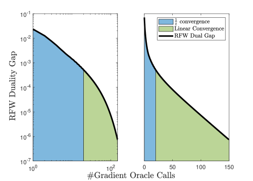
Figure 1: Numerical convergence of the RFW algorithm’s iterates (Algo. 1) for minimizing a quadratic function over a double geodesic strongly convex set in a unit sphere. The dimension of the problem is $n=500$, $x_{c}$ is a vector of ones, and the function $f$ is a random quadratic function parametrized as $f(x)\triangleq\|A(x-x^{\star})\|^{2}$, where $A$ is a random $250\times 500$ matrix, and $x^{\star}$ is generated at random such that $\operatorname{dist}(x^{\star},x_{c})\leq\pi/2$. The parameter $R$ is set such that $R=0.9\operatorname{dist}(x^{\star},x_{c})$, which ensures that the solution lies on the boundary, and therefore, there exists $c>0$ s.t. $\operatorname{argmin}_{x\in\mathcal{C}}\|\nabla f(x)\|_{x}>c$. As predicted by Theorem 7.2, the rate is locally linear.

This section presents a numerical experiment illustrating the rates stated in Theorem 7.2. Let the manifold $\mathcal{M}$ be $\mathbb{S}^{n-1}$, the unit sphere embedded in $\mathbb{R}^{n}$. Let us consider the following problem.

$$\min_{x\in\mathbb{S}^{n-1}}f(x),\qquad\text{subject to}\;\;\operatorname{dist}(x,x_{c})\leq R.$$ (28)

Owing to the symmetries of the sphere, the linear minimization oracle for (28) can be formulated as a simple one-dimensional problem (Proposition 9.2). The solution is computed using the function fminbnd from Matlab. The experimental results have been reported in Figure 1, wherein the two regimes (global rate of $O(t^{-1})$ and locally linearly convergent) are clearly distinguishable.

This problem appears, for instance, when training a neural network with spherical constraints over a hierarchical dataset.

Example 7.5 (Hierarchical neural network with sphere constraints).

Scieur and Kim [57] trained a neural network on a hierarchical dataset: “We force the classifier (hyperplane) of each class to belong to a sphere manifold, whose center is the classifier of its super-class”. Hence, in the case wherein one wants to fine-tune the last layer of such an architecture, the problem can be formulated as in (28), where $x_{c}$ is the separating hyperplane of the super-class, $R$ is a user-defined parameter, and $f(x)$ is the loss of the neural network parametrized by $x$ over the dataset.

8 Examples of Riemannian Strongly Convex Sets: Balls with Restricted Radius

The Riemannian strongly convex set, in Equation 6, is the most restrictive of our definitions. It implies that, for all points $x$ in the set $\mathcal{C}$, the logarithmic image of $\mathcal{C}$ around $x$, i.e., $\operatorname{Exp}^{-1}_{x}(\mathcal{C})$, is strongly convex in the Euclidean sense. Intuitively, we can expect that such a situation arises when the logarithmic map $\operatorname{Exp}^{-1}_{x}$ does not affect the shape of $\mathcal{C}$ too much, which is the case when the sectional curvature of $\mathcal{M}$ is bounded and the set $\mathcal{C}$ is not too large.

In this section, we show that some level sets of the function $x\mapsto\frac{1}{2}d(x,x_{0})^{2}$ are Riemannian strongly convex. Before proving the main theorem, we first introduce some concepts and two known results: 1) distance functions are locally geodesically smooth and strongly convex [45], and 2) locally, Euclidean pulled-back functions of geodesically smooth, strongly convex functions are smooth and strongly convex in the Euclidean sense [20].

8.1 Bounded curvature

In the following, we make an assumption regarding the curvature of our manifolds. Let us recall that, given a $two$-dimensional subspace $V\subseteq T_{x}\mathcal{M}$ of the tangent space of a point $x$, the sectional curvature at $x$ with respect to $V$ is defined as the Gauss curvature for the surface $\operatorname{Exp}_{x}(V)$ at $x$. The Gauss curvature at a point $x$ can be defined as the product of the maximum and minimum curvatures of the curves resulting from intersecting the surface with planes that are normal to the surface at $x$. See more details on the curvature tensor $\mathfrak{R}$ in [52]. Our assumption is as follows.

Assumption 8.1.

The sectional curvatures of $\mathcal{M}$ are contained in the interval $[\kappa_{\min},\,\kappa_{\max}]$ and the covariant derivative of the curvature tensor is bounded as $\|\nabla\mathfrak{R}\|\leq F$.

This assumption is not overly restrictive. The majority of the applications of Riemannian optimization are in locally symmetric spaces, which satisfy $\nabla\mathfrak{R}=0$, for instance, constant curvature spaces, the SPD matrix manifold with the usual metric, $\operatorname{SO}(n)$, and the Grasmannian manifold [43].

8.2 Strong Convexity and Smoothness of Distance Functions

We now state a fact regarding the smoothness and strong convexity of the distance squared to a point, that is central to many Riemannian optimization algorithms. In the sequel, we use the notation $K\stackrel{{\scriptstyle\mathrm{\scriptscriptstyle def}}}{{=}}\max\{\lvert\kappa_{\min}\rvert;\,\kappa_{\max}\}$).

Proposition 8.2.

(See [45]) Let us consider a uniquely geodesic Riemannian manifold $\mathcal{M}$ of sectional curvature bounded in $[\kappa_{\min},\kappa_{\max}]$ and a ball $B_{x_{0}}(r)$ in $\mathcal{M}$ of radius $r$ centered at $x_{0}$. The function $x\mapsto\frac{1}{2}d(x,x_{0})^{2}$ is then $\delta_{r}$-strongly convex and $\zeta_{r}$-smooth in $B_{x_{0}}(r)$, where $\delta_{r}$ and $\zeta_{r}$ are the geometric constants defined by

$$\zeta_{r}\stackrel{{\scriptstyle\mathrm{\scriptscriptstyle def}}}{{=}}\begin{cases}r\sqrt{\lvert\kappa_{\min}\rvert}\coth(r\sqrt{\lvert\kappa_{\min}\rvert})&\text{ if }\kappa_{\min}\leq 0\\ 1&\text{ if }\kappa_{\min}>0\\ \end{cases};\quad\delta_{r}\stackrel{{\scriptstyle\mathrm{\scriptscriptstyle def}}}{{=}}\begin{cases}1&\text{ if }\kappa_{\max}\leq 0\\ r\sqrt{\kappa_{\max}}\cot(r\sqrt{\kappa_{\max}})&\text{ if }\kappa_{\max}>0\\ \end{cases}$$ (29)

In the case of Hadamard manifolds, $\delta_{r}=1$ and $\zeta_{r}\in[r\sqrt{\lvert\kappa_{\min}\rvert},r\sqrt{\lvert\kappa_{\min}\rvert}+1]$.

8.3 Smoothness and Strong Convexity of Euclidean Pulled-Back Function

Under 8.1, [20, Proposition 6.1] showed that the Euclidean pulled-back function $x\mapsto f(\operatorname{Exp}_{x_{0}}(x))$ of a smooth, strongly convex function $f$ defined in a ball of restricted radius in $\mathcal{M}$ is also smooth, strongly convex (in the Euclidean sense) in a ball of the same radius.

Proposition 8.3.

(Informal, see [20, Proposition 6.1] for details). Let $\mathcal{M}$ be a uniquely geodesic Riemannian manifold that satisfies 8.1 and that contains $\mathcal{B}(x_{\text{ref}},r)$ defined as

$$\mathcal{B}(x_{\text{ref}},r):\{x\in\mathcal{M}:d(x,x_{\text{ref}})\leq r\},\qquad\text{and let}\qquad\mathcal{B}_{x_{\text{ref}}}(0,r):\{v\in\mathcal{T}_{x_{\text{ref}}}\mathcal{M}:\|v\|\leq r\}.$$

As shown above, we also defined the pulled-back ball to $\mathcal{T}_{x_{\text{ref}}}\mathcal{M}$. Let us assume the function $f:\mathcal{M}\rightarrow\mathbb{R}$ is $L$-smooth, $\mu$-strongly geodesically convex in the ball $\mathcal{B}(x_{\text{ref}},r)$, and has its minimizer $x^{\star}\in\mathcal{B}(x_{\text{ref}},r)$. Then, if

$$r\leq\frac{\mu}{L}\min\left\{\frac{1}{4K},\frac{K}{4F}\right\},$$

the pulled-back Euclidean function $x\mapsto f(\operatorname{Exp}_{x_{0}}(x))$ is $\frac{3}{2}L$-smooth, and $\frac{1}{2}\mu$-strongly convex over the ball $\mathcal{B}_{x_{\text{ref}}}(0,r)$.

One can relax the assumption of the minimizer being in the ball as this is only used to show that the Lipschitz constant of the function in the ball is at most $2Lr$. For instance, if the distance between the minimizer and $x_{\text{ref}}$ is $R$, the Lipschitz constant can be bounded by $O(LR)$, and we could use this bound to conclude a similar statement.

8.4 Main result

Using Propositions 8.2 and 8.3, we can prove that balls and other sets obtained from level sets of smooth and strongly g-convex functions in small regions are Riemannian strongly convex.

Theorem 8.4.

Let $\mathcal{M}$ be a uniquely geodesic Riemannian manifold that satisfies 8.1, and let the function $f:x\mapsto\frac{1}{2}d(x,x_{0})^{2}$, $x_{0}\in\mathcal{M}$. Then, the level sets

$$\mathcal{C}_{r}=\{x\in\mathcal{M}:f(x)\leq\frac{1}{2}r^{2}\}$$

are Riemannian strongly convex if $r\leq\frac{1}{2}\frac{\delta_{r}}{\zeta_{r}}\min\{\frac{1}{4K},\frac{K}{4F}\}$, where $\zeta_{r}$ and $\delta_{r}$ are the smoothness and strong convexity parameters of the function $\frac{1}{2}d(\cdot,x_{0})^{2}$ in $\mathcal{C}_{r}$ (see Equation 29).

Proof.

In this setting, pulling the function back to the tangent space of any point in $\mathcal{C}_{r}$ results in a Euclidean function that is strongly convex and smooth with condition number $O(\zeta_{r}/\delta_{r})$ in $\mathcal{C}_{r}$. Furthermore, for any point $x\in\mathcal{C}_{r}$, the function $\hat{f}_{x}:\operatorname{Exp}^{-1}_{x}(\mathcal{C}_{r})\to\mathbb{R}$ defined as $y\mapsto f(\operatorname{Exp}_{x}(y))$ for any $y\in\operatorname{Exp}^{-1}_{x}(\mathcal{C}_{r})$ is strongly convex with the parameter $\delta_{r}/2$, and in particular, $\operatorname{Exp}^{-1}_{x}(\mathcal{C}_{r})$ is a strongly convex set. It should be noted that we considered that the distance from $x$ to any point in $\mathcal{C}_{r}$ is at most $2r$. ∎

This implies that Riemannian balls in these generic manifolds are geodesic strongly convex sets. We note that the greatest $r$ that satisfies the condition in Theorem 8.4 is roughly a constant, considering constant curvature bounds. Being able to optimize in these sets is important as Martínez-Rubio [44] proved that one can reduce global geodesically convex optimization to the optimization over these sets.

9 Example of a Simple Linear Minimization Oracle

When the curvature is constant (spheres or hyperbolic spaces) and the domain is a ball, the linear minimization oracle can be simplified into a one-dimensional problem.

Theorem 9.1 (Linear minimization oracle in a ball in a constant curvature manifold).

Let $\bar{B}\stackrel{{\scriptstyle\mathrm{\scriptscriptstyle def}}}{{=}}\mathcal{B}(x_{0},r)\subset\mathcal{M}$ be a closed Riemannian ball in a manifold $\mathcal{M}$ of a constant sectional curvature. If the curvature $K$ is positive, let us assume $r<\frac{\pi}{2\sqrt{K}}$, so that the ball is uniquely geodesically convex. Given a point $x$ and a direction $v\in T_{x}\mathcal{M}$, we define

$$\Gamma\stackrel{{\scriptstyle\mathrm{\scriptscriptstyle def}}}{{=}}\operatorname{Exp}_{x}\left(\operatorname{span}\{\operatorname{Exp}^{-1}_{x}(x_{0}),v\}\right)\cap\{x\ |d(x,x_{0})=r\}.$$

The solution of $\mathop{\rm argmin}_{z\in\bar{B}}\langle v,\operatorname{Exp}^{-1}_{x}(z)\rangle$ can then be found in $\Gamma$.

Proof.

A solution is in the first set of the definition of $\Gamma$ owing to the symmetries of the manifold. Indeed, let us assume there is a solution $z$, such that

$$z\notin\operatorname{Exp}_{x}\left(\operatorname{span}\{\operatorname{Exp}^{-1}_{x}(x_{0}),v\}\right).$$

Now, let us consider the points $\operatorname{Exp}^{-1}_{x}(z)\in T_{x}\mathcal{M}$, and $\operatorname{Exp}^{-1}_{x}(z^{\prime})\in T_{x}\mathcal{M}$, such that $z^{\prime}$ is the point resulting from the application of $\operatorname{Exp}_{x}(\cdot)$ to the symmetric of $\operatorname{Exp}^{-1}_{x}(z)$ with respect to the plane $\operatorname{span}\{\operatorname{Exp}^{-1}_{x}(x_{0}),v\}$.

Then, $z^{\prime}$ is also a solution; therefore, $\operatorname{Exp}_{x}(\frac{1}{2}\operatorname{Exp}^{-1}_{x}(z)+\frac{1}{2}\operatorname{Exp}^{-1}_{x}(z^{\prime}))$ would also be a solution, and it would be in $\operatorname{Exp}_{x}\left(\operatorname{span}\{\operatorname{Exp}^{-1}_{x}(x_{0}),v\}\right)$.

Moreover, any solution $z$ satisfies $d(x,z)=r$ because, otherwise, there exists a neighborhood around $z$ contained in $\mathcal{B}$, and we could further decrease the function value of $\langle v,\operatorname{Exp}^{-1}_{x}(\cdot)\rangle$ for some point in this neighborhood. Finally, we can parametrize $\Gamma$ as $\theta\mapsto$ the point of intersection of $\mathcal{B}$ with the geodesic segment starting at $x$ from the direction $\cos(\theta)\operatorname{Exp}^{-1}_{x}(x_{0})+\sin(\theta)v$, where $\theta\in[0,2\pi)$. Except for the degenerate case wherein $\operatorname{Exp}^{-1}_{x}(x_{0})$ is parallel to $v$, where $\Gamma$ is a single point and the solution we are looking for. ∎

A direct consequence of Theorem 9.1 is that the problem of approximating a solution of the linear max oracle can be solved by solving an alternative one-dimensional problem.

Proposition 9.2.

Let $u_{1},\,u_{2}$ be an orthonormal basis for the linear subspace $\operatorname{span}\{\operatorname{Exp}^{-1}_{x}(x_{0}),v\}$.

The solution of $\mathop{\rm argmin}_{z\in\bar{B}}\langle v,\operatorname{Exp}^{-1}_{x}(z)\rangle$ can then be obtained by solving the following one-dimensional problem.

$$\min_{\phi\in[-\pi,\pi]}\alpha(\phi)\langle v;p(\phi)\rangle,$$

where $p(\phi)$ and $\alpha(\phi)$ are defined as

$$p(\phi) =\cos(\phi)u_{1}+\sin(\phi)u_{2},\qquad\phi\in[-\pi,\pi],$$ (30)

$$\alpha(\phi) =\mathop{\rm argmin}_{\alpha>0}:\operatorname{Dist}\left(\operatorname{Exp}_{x}(\alpha p(\phi)),x_{0}\right)=r.$$ (31)

Proof.

The proof is immediate. The subspace $\operatorname{span}\{\operatorname{Exp}^{-1}_{x}(x_{0}),v\}$ is parametrized with polar coordinates: $p$ is a direction of the unitary norm, and $\alpha$ is the length. The non-linear equation (31) represents the smallest $\alpha$ such that $\alpha\cdot p$ intersects $\mathcal{B}(x_{0},r)$. ∎

The solution $\phi$ can be computed using a one-dimensional solver, e.g., bisection or the Newton-Raphson method. It should be noted that finding $\alpha(\phi)$ is also a one-dimensional problem, and it can also be solved using similar techniques.

In some cases, there are simple formulas for $\alpha(\phi)$, e.g., when the manifold is a sphere (Proposition 9.3).

Proposition 9.3.

Let $\mathcal{M}=\mathbb{S}^{n-1}$ be the unit sphere. The formula of Equation 31 then reads as

$$\alpha(\phi)=2\text{tan}^{-1}\left(\frac{b(\phi)+\sqrt{a^{2}+b(\phi)^{2}-c^{2}}}{a+c}\right),\quad a=x_{0}^{T}x,\quad b(\phi)=x_{0}^{T}p(\phi),\quad c=1-2\sin\left(\frac{r}{2}\right).$$

Proof.

The distance function and exponential map in the sphere read as

$$\operatorname{Dist}(x,y)=2\,\text{asin}\left(\frac{\|y-x\|}{2}\right),\qquad\operatorname{Exp}_{x}(td)=x\cos(t\|d\|)+\frac{td}{\|td\|}\sin(t\|d\|).$$

Hence, for all $x,\,y\in\mathcal{M}$,

$$\operatorname{Dist}(x,y)=2\,\text{asin}\left(\frac{\|y-x\|}{2}\right)=r,$$

$$\Rightarrow \|y-x\|=2\sin\left(\frac{r}{2}\right),$$

$$\Rightarrow \|y\|^{2}+\|x\|^{2}-2x^{T}y=4\sin^{2}\left(\frac{r}{2}\right),$$

$$\Rightarrow x^{T}y=1-2\sin^{2}\left(\frac{r}{2}\right).$$

By replacing $x,\,y$ by $\operatorname{Exp}_{x}(\alpha p),\,x_{0}$ and using the expression of the exponential map, we obtain the equation

$$x_{0}^{T}x\cos(\alpha)+x_{0}^{T}p(\phi)\sin(\alpha)=4\sin^{2}\left(\frac{r}{2}\right).$$

The desired result follows after identifying the terms $a,\,b,\,c$ in

$$a\cos(\alpha)+b\sin(\alpha)=c,$$

the solution of which is

$$\alpha=2\text{tan}^{-1}\left(\frac{b\pm\sqrt{a^{2}+b^{2}-c^{2}}}{a+c}\right)+2k\pi,\qquad k\in\mathbb{Z}.$$

∎

10 Conclusion

We presented the first definitions for strong convexity of sets in Riemannian manifolds and have provided examples of these sets. We have begun to study their relationships and expect to establish more implications in future works. Our definitions seek to be well-suited for optimization and for establishing the strongly convex nature of the set. The global linear convergence of the RFW algorithm serves as a tangible demonstration of the impact of developing a theory around the strong convexity structure of these sets.

However, most importantly, we expect the development of a strongly convex structure to be helpful when developing Riemannian algorithms in the contexts wherein the Euclidean algorithm counterpart was leveraging such a structure, e.g., in the generalized power method [36], online learning [34, 22, 9, 10], and even more broadly, in the case of the use of strongification techniques, as in [48].

Acknowledgments

David Martínez-Rubio was partially funded by the DFG Cluster of Excellence MATH+ (EXC-2046/1, project id 390685689) funded by the Deutsche Forschungsgemeinschaft (DFG). AdA would like to acknowledge support from a Google focused award, as well as funding by the French government under management of Agence Nationale de la Recherche as part of the "Investissements d’avenir" program, reference ANR-19-P3IA-0001 (PRAIRIE 3IA Institute). We would like to thank Editage (www.editage.co.kr) for English language editing.

Appendix A Technical Proposition and Lemmas

A.1 Double Geodesic Strong Convexity implies Riemannian Scaling Inequality

Proposition A.1 (Double Geodesic Str. Cvx. implies Riemannian Scaling Inequality).

Let $\mathcal{C}\subset\mathcal{M}$ be a double geodesic $\alpha$-strongly convex set (Definition 3.4) in a complete connected Riemannian manifold $\mathcal{M}$. Let us assume that the double exponential map operator (Definition 6.1) is such that

$$h_{x}(u,v)=u+v,~{}~{}\forall(u,v)\in T_{x}\mathcal{M}.$$ (32)

The Riemannian scaling inequality in Definition 3.5 is then satisfied.

Proof.

Let us consider $x\in\mathcal{C}$, $g\in T_{x}\mathcal{M}$, and $v\in\mathcal{C}$ s.t.

$$v\in\underset{z\in\mathcal{C}}{\operatorname{argmax}}\langle g;\operatorname{Exp}^{-1}_{x}(z)\rangle_{x}.$$

Then, by (15), which is equivalent to Definition 3.4 with $t=1/2$, we have $\operatorname{Exp}_{\gamma_{x,v}(1/2)}\Big{(}\frac{\alpha}{4}d^{2}(x,v)z\Big{)}\in\mathcal{C}$, where $\gamma_{x,v}(\cdot)$ is the geodesic joining $x$, and $v$ and $z$ are a unit norm vector in $T_{\gamma_{x,v}(1/2)}\mathcal{M}$. Then, by optimality of $v$, for any $z\in T_{\gamma_{x,v}(1/2)}\mathcal{M}$ with $\|z\|_{\gamma_{x,v}(1/2)}=1$, we have

$$\Big{\langle}g;\operatorname{Exp}^{-1}_{x}(v)\Big{\rangle}_{x}\geq\Big{\langle}g;\operatorname{Exp}^{-1}_{x}\Big{(}\operatorname{Exp}_{\gamma_{x,v}(1/2)}\big{(}\frac{\alpha}{4}d^{2}(x,v)z\big{)}\Big{)}\Big{\rangle}_{x}.$$

Let us first recall that, by definition of the exponential map, for the geodesic $\gamma_{x,v}$ and any $t\in[0,1]$, we have $\operatorname{Exp}_{x}(t\gamma^{\prime}_{x,v}(0))=\gamma_{x,v}(t)$ such that we can write

$$\Big{\langle}g;\operatorname{Exp}^{-1}_{x}(v)\Big{\rangle}_{x}\geq\Big{\langle}g;\operatorname{Exp}^{-1}_{x}\Big{(}\operatorname{Exp}_{\operatorname{Exp}_{x}(\frac{1}{2}\gamma^{\prime}_{x,v}(0))}\big{(}\frac{\alpha}{4}d^{2}(x,v)z\big{)}\Big{)}\Big{\rangle}_{x}.$$ (33)

We can hence write this in terms of the double exponential map and subsequently in terms of the exponential operator map. We use

$$\operatorname{Exp}_{\operatorname{Exp}_{x}(\frac{1}{2}\gamma^{\prime}_{x,v}(0))}\big{(}\frac{\alpha}{4}d^{2}(x,v)z\big{)}=\operatorname{Exp}_{x}\Big{(}\frac{1}{2}\gamma^{\prime}_{x,v}(0);\big{(}\Gamma_{x}^{\gamma_{x,v}(1/2)}\big{)}^{-1}(\frac{\alpha}{4}d^{2}(x,v)z)\Big{)}.$$

Hence, on using the assumption (32) on the exponential operator, we have

$$\operatorname{Exp}_{\operatorname{Exp}_{x}(\frac{1}{2}\gamma^{\prime}_{x,v}(0))}\big{(}\frac{\alpha}{4}d^{2}(x,v)z\big{)}=\operatorname{Exp}_{x}\Big{(}\frac{1}{2}\gamma^{\prime}_{x,v}(0)+\big{(}\Gamma_{x}^{\gamma_{x,v}(1/2)}\big{)}^{-1}(\frac{\alpha}{4}d^{2}(x,v)z)\Big{)}.$$

When plugging the last equality in (33), we obtain

$$\Big{\langle}g;\operatorname{Exp}^{-1}_{x}(v)\Big{\rangle}_{x}\geq\frac{1}{2}\Big{\langle}g;\gamma^{\prime}_{x,v}(0)\Big{\rangle}_{x}+\Big{\langle}g;\big{(}\Gamma_{x}^{\gamma_{x,v}(1/2)}\big{)}^{-1}(\frac{\alpha}{4}d^{2}(x,v)z)\Big{\rangle}_{x}.$$

It should be noted that $\gamma^{\prime}_{x,v}(0)=\operatorname{Exp}^{-1}_{x}(v)$, such that

$$\Big{\langle}g;\operatorname{Exp}^{-1}_{x}(v)\Big{\rangle}_{x}\geq 2\Big{\langle}g;\big{(}\Gamma_{x}^{\gamma_{x,v}(1/2)}\big{)}^{-1}(\frac{\alpha}{4}d^{2}(x,v)z)\Big{\rangle}_{x}.$$

Wth $\Big{(}\Gamma_{x}^{y}\Big{)}^{-1}=\Gamma_{y}^{x}$ and the isometry property of $\Gamma_{x}^{\gamma_{x,v}(1/2)}$, we have

$$\Big{\langle}g;\Gamma_{\gamma_{x,v}(1/2)}^{x}\big{(}\frac{\alpha}{4}d^{2}(x,v)z\big{)}\Big{\rangle}_{x} = \Big{\langle}\Gamma_{\gamma_{x,v}(1/2)}^{x}\Gamma_{x}^{\gamma_{x,v}(1/2)}g;\Gamma_{\gamma_{x,v}(1/2)}^{x}\big{(}\frac{\alpha}{4}d^{2}(x,v)z\big{)}\Big{\rangle}_{x}$$ (34)

$$= \Big{\langle}\Gamma_{x}^{\gamma_{x,v}(1/2)}g;\frac{\alpha}{4}d^{2}(x,v)z\Big{\rangle}_{\gamma_{x,v}(1/2)}.$$ (35)

Hence, for any $z$ of a unit norm in $T_{\gamma_{x,v}(1/2)}\mathcal{M}$, we obtain

$$\Big{\langle}g;\operatorname{Exp}^{-1}_{x}(v)\Big{\rangle}_{x} \geq 2\Big{\langle}\Gamma_{x}^{\gamma_{x,v}(1/2)}g;\frac{\alpha}{4}d^{2}(x,v)z\Big{\rangle}_{\gamma_{x,v(1/2)}}$$ (36)

$$= \frac{\alpha}{2}d^{2}(x,v)\Big{\langle}\Gamma_{x}^{\gamma_{x,v}(1/2)}g;z\Big{\rangle}_{\gamma_{x,v(1/2)}}.$$ (37)

Furthermore, by maximizing over $z$, for the best $z^{*}$, we obtain

$$\Big{\langle}\Gamma_{x}^{\gamma_{x,v}(1/2)}g;z^{*}\Big{\rangle}_{\gamma_{x,v(1/2)}}=\|\Gamma_{x}^{\gamma_{x,v}(1/2)}g\|_{\gamma_{x,v}(1/2)}.$$

Then, because the parallel transport $\Gamma_{x}^{\gamma_{x,v}(1/2)}$ is an isometry, we finally have

$$\Big{\langle}g;\operatorname{Exp}^{-1}_{x}(v)\Big{\rangle}_{x}\geq\frac{\alpha}{2}d^{2}(x,v)\|\Gamma_{x}^{\gamma_{x,v}(1/2)}\nabla f(x)\|_{\gamma_{x,v}(1/2)}=\frac{\alpha}{2}d^{2}(x,v)\|g\|_{x}.$$

∎

A.2 Proof of Smoothness Property Lemma

First, we introduce the Fenchel conjugate of a function defined on a manifold.

Definition A.2.

[8] Let us Suppose that $f:\mathcal{C}\rightarrow\mathbb{R}$, where $\mathcal{C}\subset\mathcal{M}$ is a strictly convex set, where $\mathcal{M}$ is a Cartan-Hadamard manifold. For $m\in\mathcal{M}$, the $m$-Fenchel conjugate of $f$ is defined as the function $f_{m}^{*}:T_{m}^{*}\mathcal{M}\rightarrow\mathbb{R}$ such that

$$f_{m}^{*}(\xi_{m}):=\sup_{x\in T_{m}\mathcal{M}}\left\{\langle\xi_{m},\,x\rangle-f\left(\operatorname{Exp}_{m}x\right)\right\},$$ (38)

where $T_{m}^{*}\mathcal{M}$ is the cotangent bundle of $T_{m}\mathcal{M}$

In particular, we need the following property.

Lemma A.3.

[8, lem. 3.7] Let us suppose that $f,g:\mathcal{C}\rightarrow\mathbb{R}$ are proper functions, where $\mathcal{C}\subset\mathcal{M}$ is a strictly convex set, and $\mathcal{M}$ is a Cartan-Hadamard manifold, and let $m\in\mathcal{C}$. Then,

$$\text{if }f(p)\leq g(p)\;\;\forall\;p\in\mathcal{C},\text{ then }f^{*}_{m}(\xi_{m})\geq g^{*}_{m}(\xi_{m})\;\;\forall\;\xi_{m}\in T_{m}^{*}\mathcal{M}.$$ (39)

We are now ready to prove Lemma 5.1.

See 5.1

Proof.

As $f$ is a geodesically smooth function, for all $p\in\mathcal{C}$, we have $f(p)\leq g(p)$, where

$$g(p)=f(x)+\langle\nabla f(x),\,\operatorname{Exp}_{x}^{-1}(p)\rangle+\frac{L}{2}d^{2}(x,p),\quad\forall p\in\mathcal{C}.$$

Therefore, according to Lemma A.3, we have $f_{m}^{*}(\xi_{m})\geq g_{m}^{*}(\xi_{m})$, for all $m\in\mathcal{M}$. Using the definition (38),

$$g_{m}^{*}(\xi_{m}) =\sup_{Z\in T_{m}\mathcal{M}}\langle\xi_{m},\,Z\rangle_{x}-g(\operatorname{Exp}_{m}(Z))$$

In the particular case wherein $m=x$, we obtain

$$g_{x}^{*}(\xi_{x}) =\sup_{Z\in T_{m}\mathcal{M}}\langle\xi_{x},\,Z\rangle-f(x)-\langle\nabla f(x),\,Z\rangle_{x}-\frac{L}{2}\|Z\|_{x}^{2}$$

$$=-f(x)+\frac{1}{2L}\|\xi_{x}-\nabla f(x)\|_{x}^{2}$$

Therefore, the inequality $f^{*}_{x}(\xi_{x})\geq g_{x}^{*}(\xi_{x})$ can be written as

$$\frac{1}{2L}\|\xi_{x}-\nabla f(x)\|_{x}^{2}\leq f^{*}_{x}(\xi_{x})+f(x).$$

In particular, at $\xi_{x}=0$, we have the desired result, as

$$f^{*}_{x}(0)=\sup_{Z\in T_{m}\mathcal{M}}\langle 0,\,Z\rangle_{x}-f(\operatorname{Exp}_{x}(Z))=\sup_{Z\in T_{m}\mathcal{M}}-f(\operatorname{Exp}_{x}(Z))=-\inf_{z\in\mathcal{C}}f(z)=-f^{*}.$$

∎

Appendix B MATLAB code for the experiments

B.1 Subroutine: Linear Max Oracle For a Ball In a Sphere

⬇

1function v = linear_max_oracle(w, x, R, x0, manifold)

2

3% Solve the problem

4% max w^Tz : z \in exp_x^{-1}(C),

5% where C := {x:dist(x,x_0)\leq R}

6% Assume that the sphere has radius = 1!

7

8% Define the two basis vector of the subspace u_1 and u_2

9u1 = w;

10u1 = u1/norm(u1);

11u2 = manifold.log(x, x0);

12u2 = u2-u1*(u1’*u2);

13

14if norm(u2) > 0

15 u2 = u2/norm(u2);

16 p = @(phi) cos(phi)*u1 + sin(phi)*u2;

17

18 alpha = @(p) solve_sincoseq(x0’*x,x0’*p,(1-2*sin(R/2)^2));

19

20 fhandle = @(phi) -(alpha(p(phi))*cos(phi)); %same minimum since w*u2 = 0.

21 options = optimset(’TolX’,eps);

22 [best_phi] = fminbnd(fhandle, -pi, pi, options);

23 v = manifold.exp(x, p(best_phi), alpha(p(best_phi)));

24else

25 alpha = solve_sincoseq(x0’*x,x0’*u1,(1-2*sin(R/2)^2)); % best direction: u1

26 v = manifold.exp(x, u1, alpha);

27end

B.2 Sample Script: Random Quadratic Over a Sphere With Ball Constraint

⬇

1% Generate the problem data.

2d = 50;

3n = 25; % Slower convergence when n < d -> non-strongly convex case

4nIter = 500;

5dualgap = zeros(1, nIter);

6

7% Manifold: this code uses manop, see https://www.manopt.org

8manifold = spherefactory(d);

9

10% Define the problem cost function and its derivatives.

11A = randn(n,d);

12A = A’*A;

13A = A/norm(A);

14xstar = manifold.rand();

15f = @(x) 0.5*(x-xstar)’*A*(x-xstar);

16mgrad = @(x) manifold.egrad2rgrad(x, A*(x-xstar));

17L = norm(A); % Worst case

18

19% Create the problem set

20x_center = manifold.rand();

21radius_ratio = 0.9; % <1: xstar is oustide

22radius_max = manifold.dist(x_center,xstar)*radius_ratio;

23setFunction = @(x) manifold.dist(x_center, x)<=radius_max;

24

25x = x_center;

26% Main loop RFW

27for i=1:(nIter-1)

28 gradx = mgrad(x);

29 v = linear_max_oracle(-gradx, x, radius_max, x_center, manifold);

30 dualgap(i) = -manifold.inner(x, gradx, manifold.log(x, v));

31

32 step_size = -manifold.inner(x, gradx, manifold.log(x, v)) / (L*manifold.dist(x, v)^2);

33 step_size = min(step_size, 1);

34 x = manifold.exp(x, manifold.log(x, v), step_size);

35end

36v = linear_max_oracle(-gradx, x, radius_max, x_center, manifold);

37dualgap(end) = -manifold.inner(x, gradx, manifold.log(x, v));

38

39% Max at eps, otherwise the result is numerically meaningless

40semilogy(1:length(dualgap), max(dualgap,eps))

41legend({’FW Dual Gap’})

References

• Ahidar-Coutrix et al. [2020] A. Ahidar-Coutrix, T. Le Gouic, and Q. Paris. Convergence rates for empirical barycenters in metric spaces: curvature, convexity and extendable geodesics. Probability theory and related fields, 177(1):323–368, 2020.
• Aleksandrov [1957] A. D. Aleksandrov. Ruled surfaces in metric spaces. Vestnik Leningrad. Univ., 1957.
• Allen-Zhu et al. [2018] Z. Allen-Zhu, A. Garg, Y. Li, R. Oliveira, and A. Wigderson. Operator scaling via geodesically convex optimization, invariant theory and polynomial identity testing. In Proceedings of the 50th Annual ACM SIGACT Symposium on Theory of Computing, pages 172–181, 2018.
• Ambrose [1956] W. Ambrose. Parallel translation of riemannian curvature. Annals of Mathematics, 1956.
• Bacák [2014] M. Bacák. Convex analysis and optimization in Hadamard spaces. de Gruyter, 2014.
• Bacak [2018] M. Bacak. Old and new challenges in hadamard spaces. arXiv preprint arXiv:1807.01355, 2018.
• Ball et al. [1994] K. Ball, E. A. Carlen, and E. H. Lieb. Sharp uniform convexity and smoothness inequalities for trace norms. Inventiones mathematicae, 115(1):463–482, 1994.
• Bergmann et al. [2021] R. Bergmann, R. Herzog, M. S. Louzeiro, D. Tenbrinck, and J. Vidal-Núñez. Fenchel duality theory and a primal-dual algorithm on riemannian manifolds. Foundations of Computational Mathematics, pages 1–40, 2021.
• Bhaskara et al. [2020a] A. Bhaskara, A. Cutkosky, R. Kumar, and M. Purohit. Online learning with imperfect hints. In International Conference on Machine Learning, pages 822–831. PMLR, 2020a.
• Bhaskara et al. [2020b] A. Bhaskara, A. Cutkosky, R. Kumar, and M. Purohit. Online linear optimization with many hints. arXiv:2010.03082, 2020b.
• Boas Jr [1940] R. P. Boas Jr. Some uniformly convex spaces. Bulletin of the American Mathematical Society, 46(4):304–311, 1940.
• Boumal [2020] N. Boumal. An introduction to optimization on smooth manifolds. Available online, Aug, 2020.
• Boumal et al. [2014] N. Boumal, B. Mishra, P.-A. Absil, and R. Sepulchre. Manopt, a matlab toolbox for optimization on manifolds. The Journal of Machine Learning Research, 15(1), 2014.
• Braun et al. [2022] G. Braun, A. Carderera, C. W. Combettes, H. Hassani, A. Karbasi, A. Mokhtari, and S. Pokutta. Conditional gradient methods. arXiv preprint arXiv:2211.14103, 2022.
• Bridson and Haefliger [2013] M. R. Bridson and A. Haefliger. Metric spaces of non-positive curvature, volume 319. Springer Science & Business Media, 2013.
• Bubeck et al. [2018] S. Bubeck, M. Cohen, and Y. Li. Sparsity, variance and curvature in multi-armed bandits. In Proceedings of Algorithmic Learning Theory, pages 111–127. PMLR, 2018.
• Burago et al. [2001] D. Burago, I. D. Burago, Y. Burago, S. Ivanov, S. V. Ivanov, and S. A. Ivanov. A course in metric geometry, volume 33. American Mathematical Soc., 2001.
• Burago et al. [1992] Y. Burago, M. Gromov, and G. Perel’man. Ad alexandrov spaces with curvature bounded below. Russian mathematical surveys, 47(2):1–58, 1992.
• Clarkson [1936] J. Clarkson. Uniformly convex spaces. Transactions of the American Mathematical Society, 40(3):396–414, 1936.
• Criscitiello and Boumal [2021] C. Criscitiello and N. Boumal. Negative curvature obstructs acceleration for geodesically convex optimization, even with exact first-order oracles. CoRR, abs/2111.13263v1, 2021. URL https://arxiv.org/abs/2111.13263v1.
• Cuturi [2013] M. Cuturi. Sinkhorn distances: Lightspeed computation of optimal transport. Advances in neural information processing systems, 26:2292–2300, 2013.
• Dekel et al. [2017] O. Dekel, A. Flajolet, N. Haghtalab, and P. Jaillet. Online learning with a hint. In Advances in Neural Information Processing Systems, pages 5299–5308, 2017.
• Demyanov and Rubinov [1970] V. F. Demyanov and A. M. Rubinov. Approximate methods in optimization problems. Modern Analytic and Computational Methods in Science and Mathematics, 1970.
• Dzhepko and Nikonorov [2008] V. Dzhepko and Y. G. Nikonorov. The double exponential map on spaces of constant curvature. Siberian Advances in Mathematics, 18(1):21–29, 2008.
• Feydy et al. [2019] J. Feydy, T. Séjourné, F.-X. Vialard, S.-i. Amari, A. Trouve, and G. Peyré. Interpolating between optimal transport and mmd using sinkhorn divergences. In The 22nd International Conference on Artificial Intelligence and Statistics, pages 2681–2690, 2019.
• Garber and Hazan [2015] D. Garber and E. Hazan. Faster rates for the frank-wolfe method over strongly-convex sets. In International Conference on Machine Learning, pages 541–549. PMLR, 2015.
• Gavrilov [2007] A. V. Gavrilov. The double exponential map and covariant derivation. Siberian Mathematical Journal, 48(1):56–61, 2007.
• Goncharov and Ivanov [2017] V. Goncharov and G. Ivanov. Strong and weak convexity of closed sets in a Hilbert space. In Operations research, engineering, and cyber security, pages 259–297. Springer, 2017.
• Gouic et al. [2019] T. L. Gouic, Q. Paris, P. Rigollet, and A. J. Stromme. Fast convergence of empirical barycenters in alexandrov spaces and the wasserstein space. arXiv preprint arXiv:1908.00828, 2019.
• Hopf and Rinow [1931] H. Hopf and W. Rinow. Über den begriff der vollständigen differentialgeometrischen fläche. Commentarii Mathematici Helvetici, 3(1):209–225, 1931.
• Hosseini and Sra [2017] R. Hosseini and S. Sra. An alternative to EM for gaussian mixture models: Batch and stochastic Riemannian optimization. CoRR, abs/1706.03267, 2017. URL http://arxiv.org/abs/1706.03267.
• Hosseini and Sra [2020] R. Hosseini and S. Sra. Recent advances in stochastic Riemannian optimization. Handbook of Variational Methods for Nonlinear Geometric Data, pages 527–554, 2020.
• Huang et al. [2016] R. Huang, T. Lattimore, A. György, and C. Szepesvári. Following the leader and fast rates in linear prediction: Curved constraint sets and other regularities. In Advances in Neural Information Processing Systems, pages 4970–4978, 2016.
• Huang et al. [2017] R. Huang, T. Lattimore, A. György, and C. Szepesvári. Following the leader and fast rates in online linear prediction: Curved constraint sets and other regularities. The Journal of Machine Learning Research, 18(1):5325–5355, 2017.
• Jost [2012] J. Jost. Nonpositive curvature: geometric and analytic aspects. Birkhäuser, 2012.
• Journée et al. [2010] M. Journée, Y. Nesterov, P. Richtárik, and R. Sepulchre. Generalized power method for sparse principal component analysis. Journal of Machine Learning Research, 11(2), 2010.
• Kakade et al. [2009] S. Kakade, K. Sridharan, and A. Tewari. On the complexity of linear prediction: Risk bounds, margin bounds, and regularization. In Advances in neural information processing systems, pages 793–800, 2009.
• Kerdreux et al. [2021a] T. Kerdreux, A. d’Aspremont, and S. Pokutta. Local and global uniform convexity conditions. arXiv preprint arXiv:2102.05134, 2021a.
• Kerdreux et al. [2021b] T. Kerdreux, A. d’Aspremont, and S. Pokutta. Projection-free optimization on uniformly convex sets. In International Conference on Artificial Intelligence and Statistics, pages 19–27. PMLR, 2021b.
• Kerdreux et al. [2021c] T. Kerdreux, L. Liu, S. Lacoste-Julien, and D. Scieur. Affine invariant analysis of frank-wolfe on strongly convex sets. In International Conference on Machine Learning, pages 5398–5408. PMLR, 2021c.
• Kerdreux et al. [2021d] T. Kerdreux, C. Roux, A. d’Aspremont, and S. Pokutta. Linear bandits on uniformly convex sets. Journal of Machine Learning Research, 22(284):1–23, 2021d.
• Lee [2018] J. M. Lee. Introduction to Riemannian manifolds. Springer, 2018.
• Lezcano-Casado [2020] M. Lezcano-Casado. Curvature-dependant global convergence rates for optimization on manifolds of bounded geometry. arXiv preprint arXiv:2008.02517, 2020.
• Martínez-Rubio [2020] D. Martínez-Rubio. Global Riemannian acceleration in hyperbolic and spherical spaces. arXiv preprint arXiv:2012.03618, 2020. URL https://arxiv.org/abs/2012.03618.
• Martínez-Rubio and Pokutta [2022] D. Martínez-Rubio and S. Pokutta. Accelerated Riemannian optimization: Handling constraints with a prox to bound geometric penalties. arXiv preprint arXiv:2211.14645, 2022. URL https://arxiv.org/abs/2211.14645.
• Mérigot et al. [2020] Q. Mérigot, A. Delalande, and F. Chazal. Quantitative stability of optimal transport maps and linearization of the 2-wasserstein space. In International Conference on Artificial Intelligence and Statistics, pages 3186–3196. PMLR, 2020.
• Meyer [1989] W. Meyer. Toponogov’s theorem and applications. Lecture Notes, Trieste, 1989.
• Molinaro [2020] M. Molinaro. Curvature of feasible sets in offline and online optimization. arXiv:2002.03213, 2020.
• Nikonorov [2013] Y. G. Nikonorov. Double exponential map on symmetric spaces. Siberian Advances in Mathematics, 23(3):210–218, 2013.
• Paris [2020] Q. Paris. The exponentially weighted average forecaster in geodesic spaces of non-positive curvature. arXiv:2002.00852, 2020.
• Paris [2021] Q. Paris. Online learning with exponential weights in metric spaces. arXiv:2103.14389, 2021.
• Petersen [2006] P. Petersen. Riemannian geometry, volume 171. Springer, 2006.
• Pisier [1975] G. Pisier. Martingales with values in uniformly convex spaces. Israel Journal of Mathematics, 20(3-4):326–350, 1975.
• Pisier [2011] G. Pisier. Martingales in Banach spaces (in connection with type and cotype). course IHP, Feb. 2–8, 2011.
• Rapcsák [2013] T. Rapcsák. Smooth nonlinear optimization in Rn. Springer Science & Business Media, 2013.
• Sakai [1996] T. Sakai. On riemannian manifolds admitting a function whose gradient is of constant norm. Kodai Mathematical Journal, 19(1):39–51, 1996.
• Scieur and Kim [2021] D. Scieur and Y. Kim. Connecting sphere manifolds hierarchically for regularization. In International Conference on Machine Learning, pages 9399–9409. PMLR, 2021.
• Sun et al. [2017] J. Sun, Q. Qu, and J. Wright. Complete dictionary recovery over the sphere II: recovery by Riemannian trust-region method. IEEE Trans. Inf. Theory, 63(2):885–914, 2017. doi: 10.1109/TIT.2016.2632149. URL https://doi.org/10.1109/TIT.2016.2632149.
• Villani [2009] C. Villani. Optimal transport: old and new, volume 338. Springer, 2009.
• Weber and Sra [2017] M. Weber and S. Sra. Riemannian optimization via frank-wolfe methods. arXiv preprint arXiv:1710.10770, 2017.
• Weber and Sra [2019] M. Weber and S. Sra. Projection-free nonconvex stochastic optimization on riemannian manifolds. arXiv preprint arXiv:1910.04194, 2019.
• Zhang and Sra [2016] H. Zhang and S. Sra. First-order methods for geodesically convex optimization. In Conference on Learning Theory, pages 1617–1638. PMLR, 2016.
• Zhang and Sra [2018] H. Zhang and S. Sra. An estimate sequence for geodesically convex optimization. In Conference On Learning Theory, pages 1703–1723. PMLR, 2018.