FRDiff: Feature Reuse for Exquisite Zero-shot Acceleration of Diffusion Models

Abstract

The substantial computational costs of diffusion models, particularly due to the repeated denoising steps crucial for high-quality image generation, present a major obstacle to their widespread adoption. While several studies have attempted to address this issue by reducing the number of score function evaluations using advanced ODE solvers without fine-tuning, the decreased number of denoising iterations misses the opportunity to update fine details, resulting in noticeable quality degradation. In our work, we introduce an advanced acceleration technique that leverages the temporal redundancy inherent in diffusion models. Reusing feature maps with high temporal similarity opens up a new opportunity to save computation without sacrificing output quality. To realize the practical benefits of this intuition, we conduct an extensive analysis and propose a novel method, FRDiff. FRDiff is designed to harness the advantages of both reduced NFE and feature reuse, achieving a Pareto frontier that balances fidelity and latency trade-offs in various generative tasks.

1 Introduction

The diffusion model has gained attention for its high-quality and diverse image generation capabilities [34, 36, 38, 33]. Its outstanding quality and versatility unlock new potentials in various applications, including image restoration [48, 23], image editing [4, 12, 46, 49, 35], conditional image synthesis [2, 10, 52, 55, 50, 54, 31], and more. However, the expensive computation cost of the diffusion model, particulary due to its dozens to hundreds of denoising steps for high-quality image generation, poses a significant obstacle to its widespread adoption. For example, while a GAN [8] can generate 50k images of size 32x32 in less than a minute, the diffusion model takes approximately 20 hours. To fully harness the benefits of diffusion models in practice, this performance drawback must be addressed.

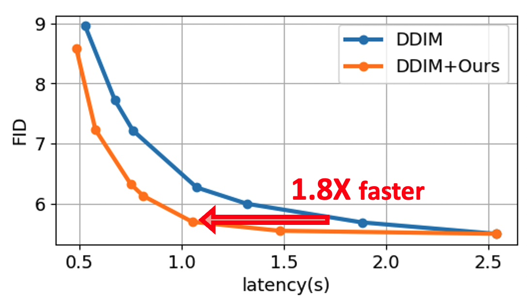
Figure 1: FID-Latency trade-off by using DDIM [43] and Ours in CelebA-HQ dataset. Our method can further accelerate advanced ODE solver like DDIM, especially in low-FID region.

Recently, many studies have proposed methods to reduce the computational cost of diffusion models. A representative approach involves a zero-shot sampling method [43, 24, 44], which typically employs advanced ODE or SDE solvers capable of maintaining quality with a reduced number of score function evaluations (NFE). They demonstrate the potential for acceleration without fine-tuning, but performance improvement achievable within the accuracy margin is not sufficient. On the other hand, there is another direction that utilizes a learning-based sampling method [39, 30, 45, 25], applying fine-tuning to maintain generation quality with a reduced NFE. However, the requirement of fine-tuning, such as additional resources and a complex training pipeline, make it challenging to use in practice. To realize practical benefits with minimal constraints, we need more advanced zero-shot methods with higher potential.

In this work, we focus on an important aspect of the diffusion model that has not been utilized in previous studies. Since diffusion models involve iterative denoising operations, the feature maps within the diffusion model exhibit temporal redundancy. According to our extensive analysis, specific modules within diffusion models show high similarity in their feature maps across adjacent frames. By reusing these intermediate feature maps with higher temporal similarity, we can significantly reduce computation overhead while maintaining output quality. Building on this insight, we propose a new optimization approach, named feature reuse (FR).

However, the naive use of FR doesn’t guarantee superior performance compared to the conventional reduced NFE method. Our thorough experiments reveal that FR has distinctive characteristics compared to the reduced NFE method, and both methods can be used in harmony to compensate for each other’s drawbacks and maximize the benefits we can achieve. Overall, we propose a comprehensive method named FRDiff, designed to harness the strengths of both low NFE and FR. In particular, we introduce a score mixing method that enables FRDiff to generate high-quality output with fine details while reducing computation overhead. This approach can be applied to any diffusion model without the need for fine-tuning in existing frameworks with minimal modification.

We conduct extensive experiments to validate the effectiveness of FRDiff on various tasks in a zero-shot manner. We can achieve up to a 1.8x acceleration without compromising output quality across a range of tasks, including a task-agnostic pretrained model for text-to-image generation, as well as task-specific fine-tuned models for super resolution and image inpainting.

2 Related Works

2.1 Diffusion Models

The diffusion model, introduced in [42], defines the forward diffusion process by gradually adding Gaussian noise at each time step. Conversely, the reverse process generates a clean image from random noise by gradually removing noise from the data. In DDPM [15], the authors simplified the diffusion process using a noise prediction network $\epsilon_{\theta}(x_{t},t)$ and reparameterized the complex ELBO loss [19] into a straightforward noise matching loss.

On the other hand, in [44], it was proposed that the forward process of the diffusion model can be transformed into a Stochastic Differential Equation (SDE). They also identified a corresponding reverse SDE for the reverse process of the diffusion model. Furthermore, it was revealed that the noise prediction is equivalent to the score of the data distribution, $\nabla_{x}p(x)$. Recently, Classifier-Free Guidance (CFG) [14] has been introduced to guide the score toward a specific condition $c$. In the CFG sampling process, the score is represented as a linear combination of unconditional and conditional scores.

As the proposed FRDiff is designed based on the temporal redundancy resulting from the iterative nature of the diffusion process, it can be applied to all the aforementioned methods, providing significant performance benefits regardless of their specific details.

2.2 Diffusion Model Optimization

Numerous studies have aimed to address the slow generation speed of the diffusion models. The primary factor of this drawback is the iterative denoising process that requires a large NFE. Consequently, many studies have focused on reducing NFE, which can be broadly categorized into two groups: zero-shot sampling [43, 56, 24, 17, 26, 51, 27], which apply optimization to the pre-trained model, and learning-based sampling [39, 30, 28, 25], which entails an additional fine-tuning.

Zero-shot sampling methods typically employ advanced Ordinary Differential Equation (ODE) solvers capable of maintaining generation quality even with a reduced NFE. For instance, DDIM [43] successfully reduced NFE by extending the original DDPM to a non-Markovian setting and eliminating the stochastic process. Furthermore, methods that utilize Pseudo Numerical methods [24], Second-order methods [17], and Semi-Linear structures [26, 27] have been proposed to achieve better performance. Learning-based sampling finetunes the model to perform effectively with fewer NFE. For example, Progressive Distillation [39] distills a student model to achieve the same performance with half of NFE. Recently, the consistency model [45, 28] successfully reduced NFE to 1-4 by predicting the trajectory of the ODE.

In addition, there are studies aimed at optimizing the backbone architecture of the diffusion model. These studies involve proposing new diffusion model structures [36, 18], as well as lightweighting the model’s operations through techniques such as pruning [7], quantization [21, 41], and attention acceleration [3].

In this work, we primarily focus on enhancing the benefit of zero-shot model optimization for diffusion models. Therefore, we conduct experiments compared to the corresponding baselines; however, please note that the proposed method could apply along with other learning-based or backbone optimization studies.

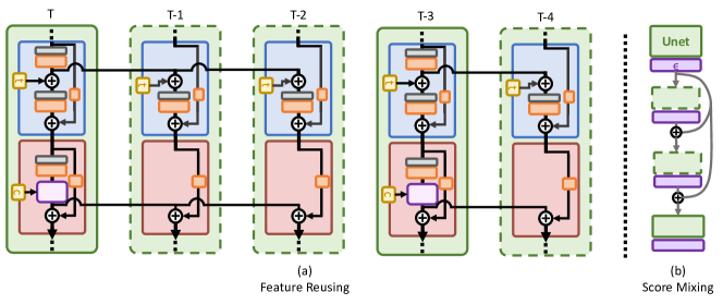
Figure 2: Overview of our method. In (a), feature maps from keyframe(t=T,T-3) are reused in next time steps. The skip interval is 3 in this example. In (b), we briefly represent our score mixing method.

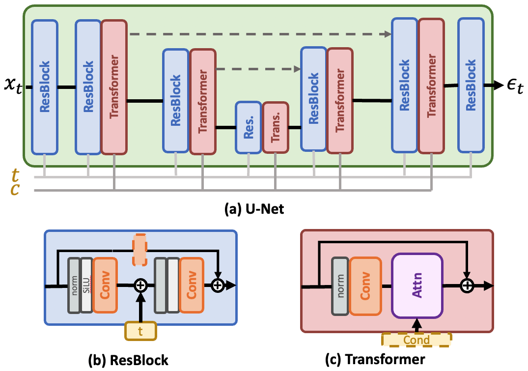
Figure 3: The representative structure of the U-net [37] for Diffusion models consists of a repeated stack of Residual [11] and Transformer blocks [47].

3 Motivation of Feature Reuse

In this study, we introduce the idea of feature reuse (FR) as an innovative approach to expand the scope of model optimization for diffusion models. FR possesses distinct attributes compared to the lowering NFE, enabling a synergistic effect when used together. This combination results in superior performance at equivalent quality levels. In this chapter, we will explain the motivations behind the proposal of FR and discuss the expected advantages of this method.

3.1 Potential of FR: Temporal Similarity

In Fig. 3 (a), we provide a brief overview of the U-net [37] architecture used in diffusion models. As depicted in the figure, it comprises multiple stacks of residual [11] and transformer blocks [47]. To generate high-quality images, this U-net block is repeatedly employed, taking the noisy image $x_{t}$ at time step $t$ as input and predicting the denoised output $\epsilon_{t}$, which is subsequently added to $x_{t}$.

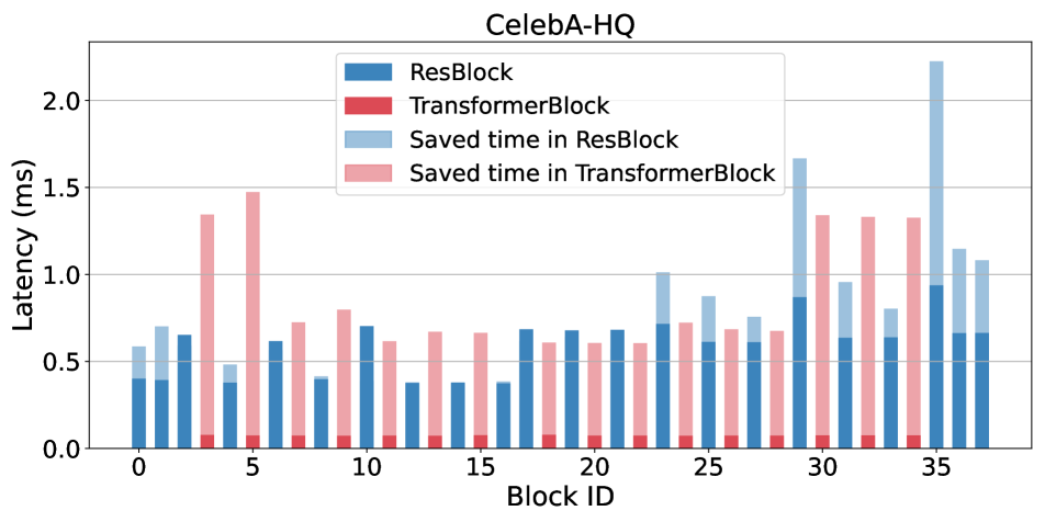
(a) LDM-4

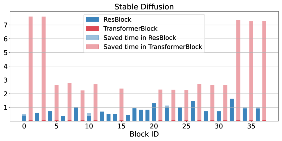
(b) Stable Diffusion

Figure 4: The detailed analysis of the skippable latency by FR technique for (a) LDM-4 [36] and (b) Stable Diffusion.

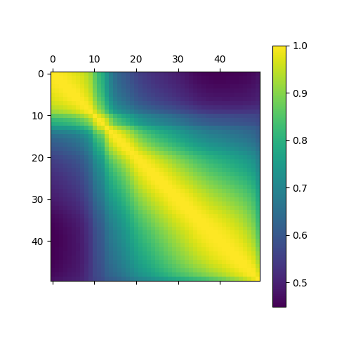
(a) ResBlock

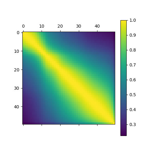
(b) Transformer Block

Figure 5: The heatmap visualization of temporal similarity of feature map on residual and transformer blocks in the stable diffusion model. The x and y axes represents timesteps, and the scores reflects the cosine similarity of outputs at different timesteps.

In the previous approaches lowering NFE, the U-net computation was selectively skipped, generating images only sparsely at certain timesteps. However, this approach proved to be too coarse-grained, leading to a noticeable degradation in output quality under insufficient NFE conditions due to the missed opportunity for detail compensation.

In FR, we shift our focus towards a finer-grained skipping and reuse strategy within the U-net structure. Our motivation for this shift arises from the temporal redundancy resulting from the repetitive use of denoising processes, leading to high similarity among neighboring features. To validate this assumption, we initially conducted an analysis measuring the temporal similarity of feature maps in a stable diffusion model. We extensively assessed various locations within the U-net structure and attempted to identify the structural basis for particularly high temporal similarity.

Based on empirical observations, we noticed that the output of the first convolution within the residual block and the output of the attention block within the transformer block exhibited a high temporal similarity in adjacent frames (within $<$ 5 timesteps), regardless of their positions within the network. Fig. 5 presents a visualization of this phenomenon for one block from each type in a stable diffusion model, clearly highlighting the strong correlation along the near diagonal elements. This observation strongly supports our idea that we can reuse previous outputs without experiencing a significant degradation in output quality.

In FR, it’s important to note that the network components having low similarity are computed as usual, and the information along the skip connection is continuously updated even when employing the FR approach. This selective computation, along with the partial reuse of feature maps, enables proper per-instance adaptation for thoughtful output generation. Fig. 2 (a) visualizes the overview of the FR method. As shown in the figure, the time step at which all computations are performed is referred to as a keyframe. Afterward, a subset of feature maps in the residual and transformer blocks is reused in the subsequent time step. It’s worth noting that the allocation of keyframes can be adjusted to maximize output quality within a given latency target. However, in this paper, we uniformly allocate keyframes to comprehensively validate the benefits of FR. The search for the optimal skip interval is a topic left for future work.

With the FR method, we can enjoy performance benefits for a pre-trained diffusion model with minimal code modifications without the need for additional fine-tuning. In Fig. 6, we demonstrate the results of applying FR to the LDM-4 ImageNet [6] 256x256 model. As shown in the figure, the quality of generated images remains nearly unchanged until the skip interval is less than 8.

3.2 Performance Benefit of Feature Reuse

Through our extensive analysis, we have empirically observed that the utilization of the FR technique holds promise in preserving output quality while reducing computational demands. However, we need to validate whether this method can indeed offer practical advantages. Therefore, we conducted a comprehensive analysis to evaluate the latency with FR on a real device (NVIDIA RTX3090).

The impact of applying FR on performance differs between the residual and transformer blocks. In the residual block, we solely skip the initial convolution operation, resulting in a latency reduction of less than 50%. On the other hand, in the case of the transformer block, we can skip the majority of computations, including attention and embedding operations, and only need to perform normalization with addition. This allows us to achieve a substantial latency reduction of up to 90% on real devices.

In Fig. 4, we depict the latency profiles of individual blocks within two Diffusion U-Net structures: LDM-4 and stable diffusion. Both models employ the residual and transformer modules as their building blocks, but their distribution of latency differs. In the LDM-4 model, the residual block and transformer block consume a roughly equal portion of execution time. However, in the case of Stable Diffusion, where higher-resolution images are generated, the transformer block accounts for a larger portion of the execution cycle. This is primarily due to the inclusion of a spatial self-attention layer in the processing of high-resolution feature maps. Consequently, the anticipated performance improvement in the LDM-4 model is somewhat less pronounced compared to that of the stable diffusion model. However, in both scenarios, when employing FR, we can achieve latency reductions of approximately 82% and 95%, respectively in the subsequent frames.

4 Comprehensive Optimization: FRDiff

As explained in the previous section, FR could provide advantages in terms of both performance and quality. However, since we are already aware of various methods for achieving performance improvements based on reducing NFE, the adoption of FR should be justified by the distinctive advantages of FR over the reduced NFE. In this section, we will elucidate the benefits of FR we have discovered and explain how we can maximize performance by leveraging these advantages. We will also provide a detailed description of our FRDiff method, which combines FR with the reduced NFE to fully harness these advantages.

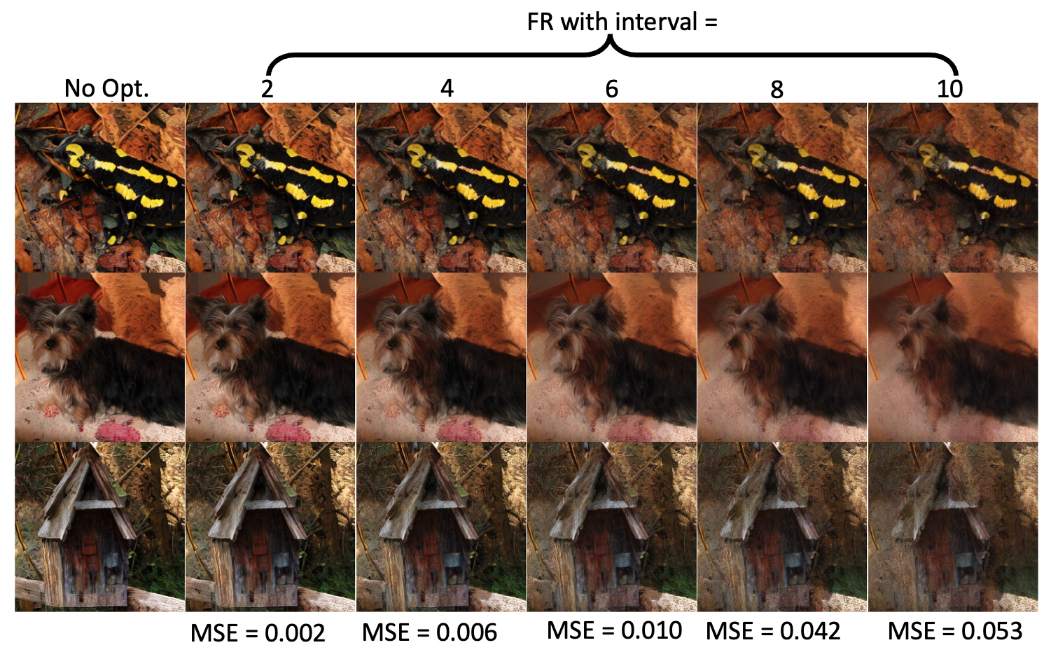
Figure 6: Generated result of FR. The quality of generated and MSE between original image remains nearly unchanged until the keyframe interval is less than 8.

4.1 Detailed Analysis of Feature Reuse

In this chapter, we aim to explore whether using FR offers any additional advantages beyond reducing NFE. To enable a direct comparison of the strengths and weaknesses of both methods, we have transformed NFE into the same representation as FR. If we consider reusing the entire output of the U-net, this can be seen as a very coarse-grained form of FR. We have confirmed that this method, which we named “Jump”, is ultimately equivalent to the case when NFE equals to the total time steps divided by skip intervals. The proof is available in the supplementary material. To ensure a clear comparison, we have conducted a detailed analysis of how both FR and Jump cause any quality degradation when increasing the skip interval.

In Fig. 7, we present the original image (a) generated with DDIM over 50 steps on LDM-4 CelebA-HQ, FR with an interval of 10 (b), and Jump with the same interval (c). Notably, only 5 key frames are used. We intentionally use a low number of key frames to observe the generation behavior under challenging conditions. In comparison to the original image (a), FR (b) effectively preserves details like hair texture but exhibits differences in color. Conversely, Jump (c) maintains color well but has a blurry image and struggles to preserve details. Our qualitative analysis reveals that both methods exhibit distinct characteristics. For a more in-depth analysis, we conducted Power Spectral Density (PSD) analysis of the generated images, as shown in Fig. 17. When we apply coarse-grained reuse, or Jump, we lose many details in the high-frequency component (Fig. 17(a)); meanwhile, when we apply FR, it loses more low-frequency components while better preserving the high-frequency component (Fig. 17(b)).

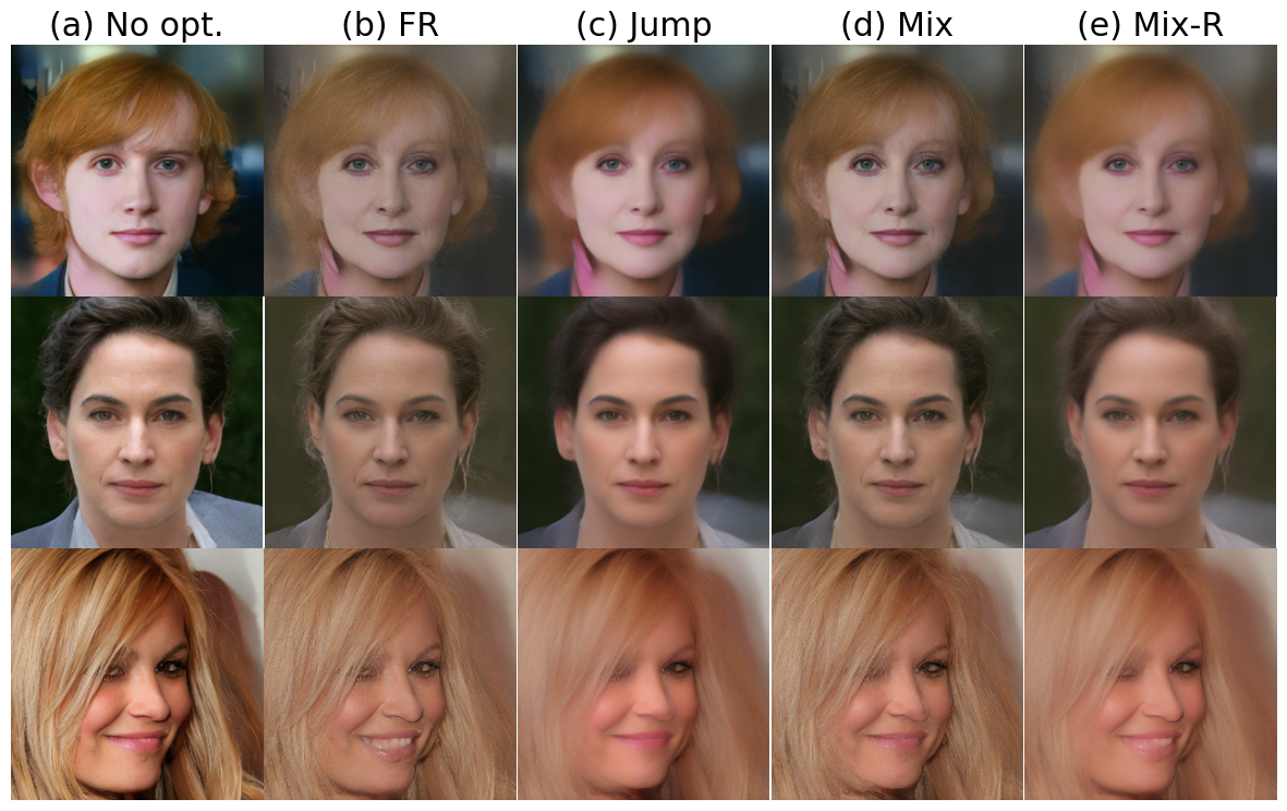
Figure 7: Generated images of CelebA-HQ [16] using various FR schemes with DDIM 50 step interval 10. While Jump (c) shows blurry image, FR (b) effectively preserve details(e.g hair texture). However, (b) tends to compromise low-frequency components such as colors. Meanwhile, our proposed score mixing (d) preserves both low and high-frequency components well, whereas the opposite, Mix-R (e) shows a decline in both components.

4.2 Key Motivation of FRDiff

Our empirical findings suggest that FR is not consistently better than Jump; they possess distinct characteristics and strengths and weaknesses. At this point, we need to pay attention to the recent finding on the generation characteristics. Recent studies [29, 5, 53, 7] have shown that in the early denoising stages, the model mainly generates coarse-grained low-frequency components. In contrast, during the later stages, it predominantly generates fine-grained high-frequency components. Therefore, by combining these operational characteristics with our observations, we devised a strategy that primarily employs Jump in the initial stages to preserve low-frequency components and then switches to FR in the later stages to retain high-frequency details. This is the core motivation of the proposed FRDiff, aims to maximize performance improvement while minimizing quality degradation.

4.3 Additional Idea: Score Mixing

To integrate the two methods, we have introduced an additional heuristic called “score mixing”. During the denoising process, we employ a linear interpolation of the scores estimated by Jump and FR, respectively, controlled by a mixing schedule $\lambda(t)$. In simpler terms, the outputs from the FR path are weighted sum with the outputs from the previous key frame. This process is represented in Eq. 1 and visually depicted in Fig. 2 (b).

$$\epsilon(t)_{mixed}=\lambda(t)*\epsilon(t)_{FR}+(1-\lambda(t))*\epsilon_{keyframe}$$ (1)

$$\lambda(t)=\frac{1}{1+e^{-\tau(t-b)}}$$ (2)

In Eq. 2, $\tau$ is temperature that controls stiffness of schedule and $b$ is bias that controls phase transition point of schedule. We empirically determine the optimal values as $\tau=30$ and $b=0.5$ and will use these values throughout the rest of the paper.

One limitation of the above method is its consistent reliance on the FR score, which reduces the performance benefits due to the continual computation of the FR path. To further accelerate the denoising process, we set $\lambda(t)$ to a hard sigmoid function as follows:

$$\lambda(t)=\max(0,\min(1,(\tau*(t-b)+2)/4)).$$ (3)

By using this $\lambda(t)$, we can skip the computation of the FR score ($\epsilon(t)_{FR}$) when $\lambda(t)=0$. In the case of conditional sampling (CFG), we simply mix the conditional score in the same way as the unconditional score, using the same $\lambda$.

Fig. 7 presents a comparison of generated images using Mix (d) and Mix-R (e). Mix-R (e) represents an experiment where we use $\lambda(-t)$ instead of $\lambda(t)$, meaning that we utilize FR in the early stage and Jump in the later stage. As shown in the figure, the Mix (d) image exhibits the highest quality, with a significant amount of detailed components compared to Jump, and well-preserved colors compared to FR. Conversely, both components show a decline in quality in the case of Mix-R (e). Additionally, Fig. 17 illustrates the PSD plots of Mix (c) and Mix-R (d). As shown in the figure, Mix effectively preserves high-frequency components compared to Jump and maintains low-frequency components well compared to Skip, while Mix-R exhibits a decline in both frequency components.

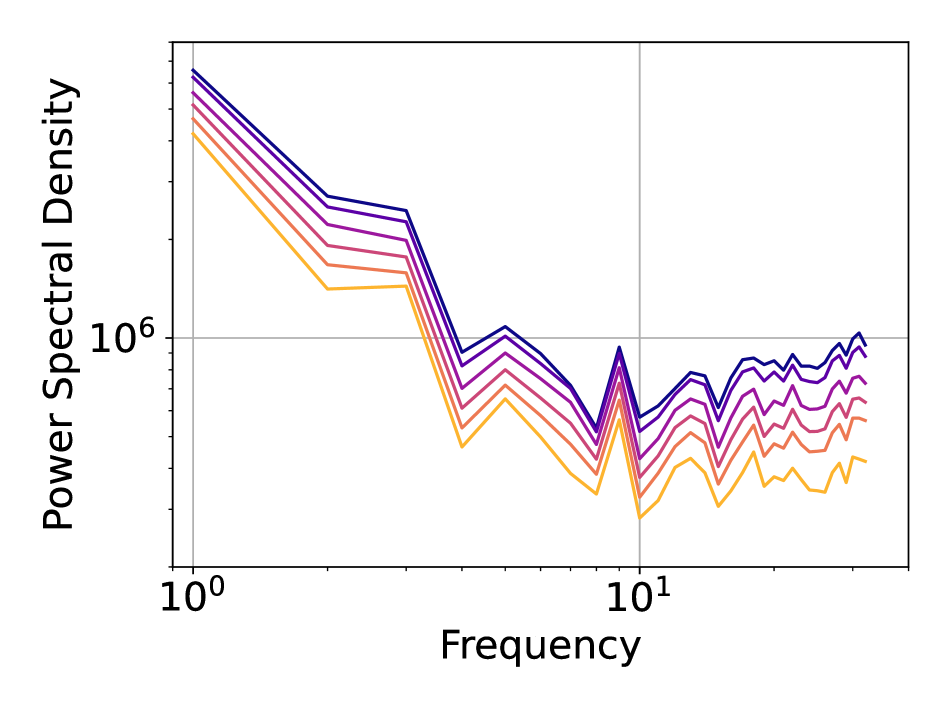
(a) Jump

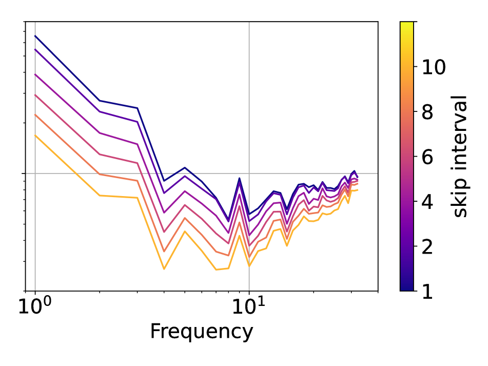
(b) FR

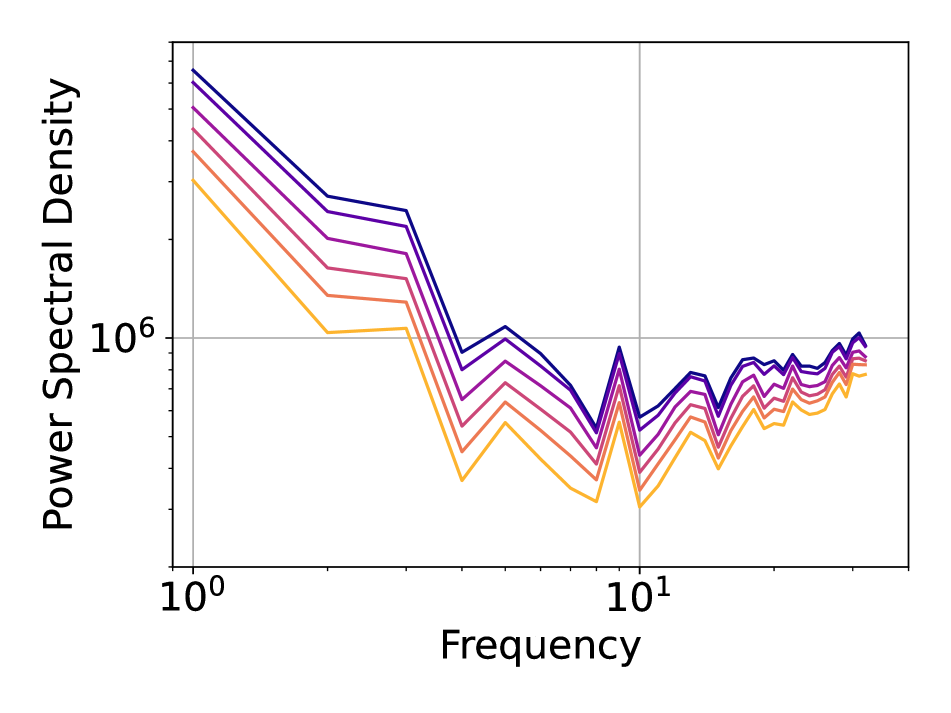
(c) Mix

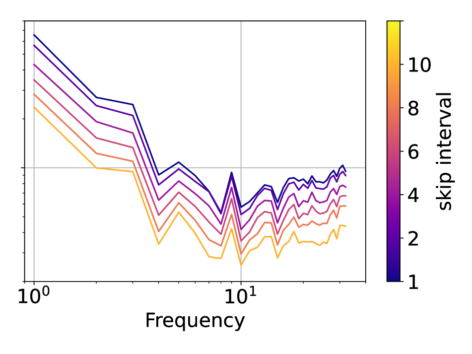
(d) Mix-R

Figure 8: Power Spectral Density(PSD) of generated Image. While Jump (a) fails to preserve high-frequency components, FR (b) effectively preserve it but lost low-frequency components. Our score mixing approach (c) preserves both low and high-frequency components well. In contrast, Mix-R (d), which follows the opposite mixing schedule, shows a decline in both components.

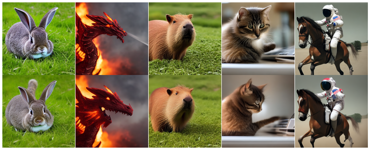
Figure 9: Text-to-Image generation results of Ours (DDIM 15 step interval 2)(Up) and DDIM (8 step) (Down) at same latency budget.

5 Experiments

5.1 Experiments Setup

To validate the effectiveness of the proposed idea, we assessed the efficacy of our method across various existing Diffusion Models, conducting experiments on two types: pixel-space [43] and latent-space models [36], using diverse datasets. We obtained the pretrained weights from the official repository, except for CIFAR-10 [20].

To evaluate our method, we conducted both qualitative and quantitative experiments. For qualitative assessment, we compared our generated images with those from the existing DDIM [43] sampler in tasks like Text-to-Image generation, Super Resolution, and Image Inpainting, employing Stable Diffusion(v1.4) for Text-to-Image, LDM-SR for Super Resolution, and LDM-Inpaint for Image Inpainting.

For quantitative evaluation, we measured the trade-off between Fréchet Inception Distance (FID) [13] and latency. FID was calculated by comparing 50,000 generated images with the training dataset. However, for Stable Diffusion, due to its training on a web-scraped large-scale image dataset [40], we used DDIM 100-step sampled images as references and measured FID with the images generated from 5000 prompts from MS-COCO [22] val set.

All experiments were conducted on a GPU server equipped with an NVIDIA GeForce RTX 3090, and latency measurements were performed using PyTorch [32] with a batch size of 1 on a GeForce RTX 3090 GPU.

5.2 Qualitative Analysis

5.2.1 Text-to-Image Generation with Stable Diffusion

Fig. 9 displays a comparison of text-to-image generation results using Stable Diffusion, with Ours (top) and DDIM (bottom) at the same latency budget, 1.16s. The prompts used for generating images were “a rabbit eating grass”, “a close-up of a fire-spitting dragon, cinematic”, “a capybara sitting in a realistic field”, “a cat on a desk” and “an astronaut riding a horse”. As illustrated in the figure, Ours consistently demonstrates superior image quality compared to DDIM. Specifically, while certain outputs produced by DDIM exhibit blurriness and a degraded structure, our model consistently preserves high-quality images, with a particular emphasis on retaining high-frequency components like fur in animals.

5.2.2 Super Resolution

To assess the effectiveness of our model in task-specific applications, we performed image synthesis, upscaling a 256x192 resolution image to 1024x768 resolution using LDM-SR. In Fig. 12, we compare our method (b) with the existing DDIM [43] sampling (a) with the same latency budget, 7.64s. As depicted in the figure, DDIM (a) recovers some details but exhibits slightly blurred image texture. In contrast, our method (b) preserves better details than DDIM (a) and includes higher-quality features. This demonstrates that our method can generate higher-quality and more detailed images than existing DDIM sampling.

Method	FID	Latency(s)
Sigmoid	5.64	1.67
Hard Sigmoid	5.67	1.49
Step Function	5.82	1.47

Table 1: Effect of $\lambda(t).$

Model	Size (MB)
CIFAR-10	5.4
LDM-4	44.4
Stable Diffusion	180.0
LDM-SR	536.2

Table 2: Memory overhead.

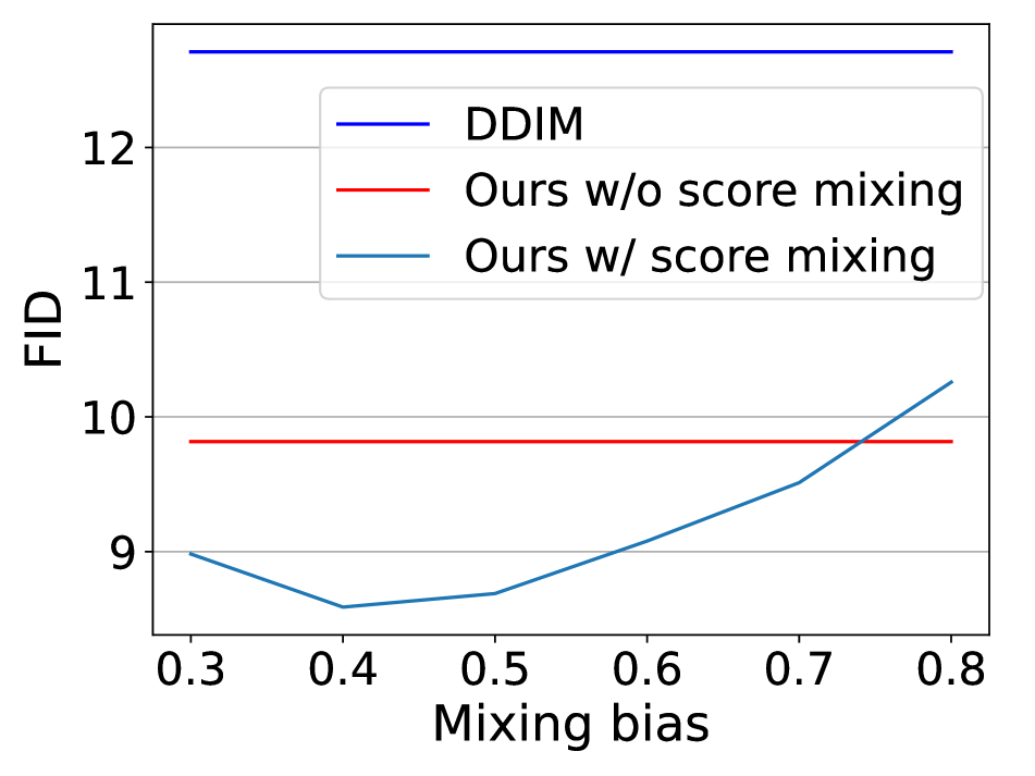
(a) Skip interval 4

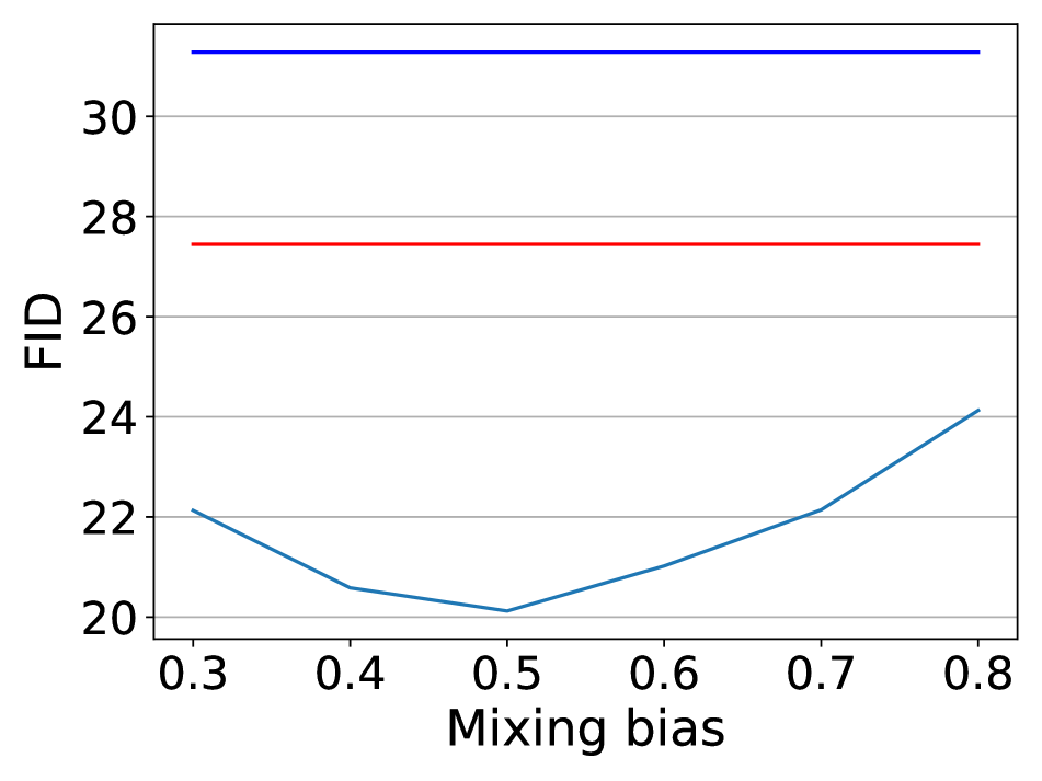
(b) Skip interval 8

Figure 10: Effect of bias in score mixing. The optimal value of bias exist around 0.4 0.6, where the generation phase shift from low frequency and high frequency.

5.2.3 Image Inpainting

In Fig. 13, we evaluate the performance of our method in Image Inpainting compared to DDIM sampling within the same latency budget, 1.16s. The image inpainting process generates content for the region corresponding to the mask image from the source image. Compared to DDIM (b), our method (c) generates higher-quality images and can effectively generate more content by considering the surrounding context. This suggests that our approach tends to recover more parts of the image efficiently when applying image inpainting with a smaller number of steps compared to DDIM.

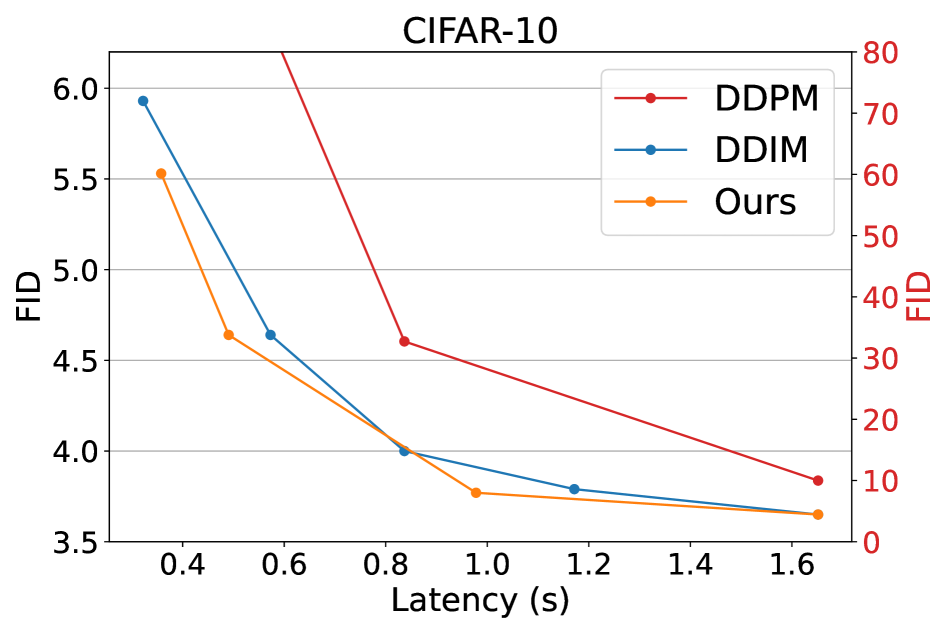
(a) CIFAR-10

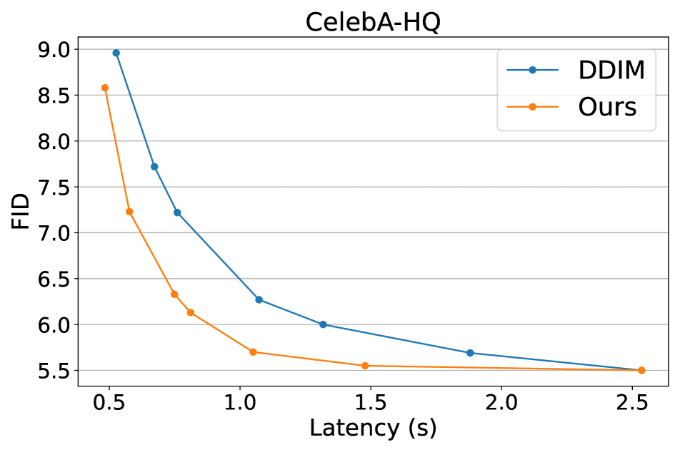
(b) LDM-CelebA-HQ

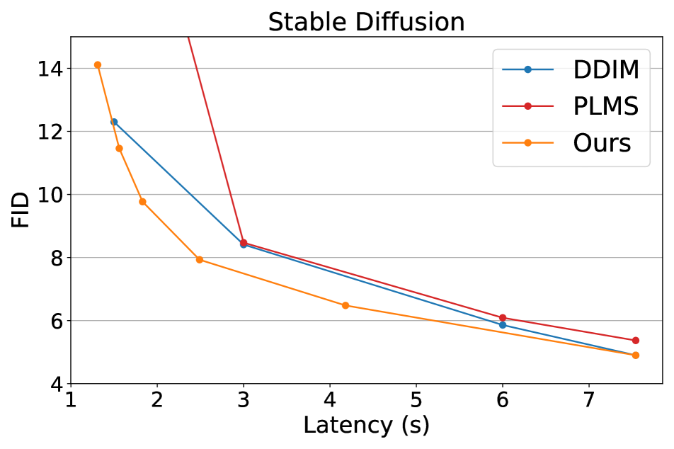
(c) Stable Diffusion

Figure 11: FID-Latency pareto plot for various models, datasets. Our method can speed up existing advanced samplers up to 1.8x.

5.3 FID-Latency Tradeoff

In Fig. 11, we plotted the FID-Latency Pareto for pixel-space CIFAR-10 [20], LDM-4 CelebA-HQ [16], and Stable Diffusion to illustrate the effectiveness of our method compared to existing sampling methods. As depicted in the figure, our method achieves significantly lower FID scores at the same latency, regardless of the architecture or dataset. Particularly, our method can achieve acceleration of up to 1.8 times at the same FID for the CelebA-HQ dataset [16] and up to 1.5 times for Stable Diffusion. However, there is only a subtle performance improvement observed in CIFAR-10, which is attributed to the limited potential for acceleration in structures.

5.4 Ablation Study

5.4.1 Score Mixing

Effect of bias In Eq. (2), the bias $b$ determines the transition point from the low-frequency phase to the high-frequency phase. To understand the impact of this bias on generation performance, we varied the bias from 0.3 to 0.8 and measured the FID score, as shown in Fig. 10. The figure illustrates that the optimal FID is achieved when the bias is around 0.4 to 0.5, which aligns with our previous observations. Additionally, there is a trend where the optimal bias value increases as the skip interval increases. This occurs because as the skip interval increases, the approximation error of FR also increases.

Effect of $\lambda(t)$ In this section, we conducted experiments to evaluate the performance variations with different scheduling functions $\lambda(t)$:(a) the sigmoid function, (b) the hard sigmoid, and (c) the step function. The performance for each $\lambda(t)$ is presented in Table 2. As observed in the table, there is little difference between the sigmoid (a) and hard sigmoid (b). Therefore, we can safely change our scheduler to (b) to obtain additional acceleration. Furthermore, when comparing sigmoid (a) with the step function (c), it is evident that sigmoid scheduling performs better. Thus, we can conclude that incorporating soft mixing has a positive impact on generation.

(a) DDIM 30 Step

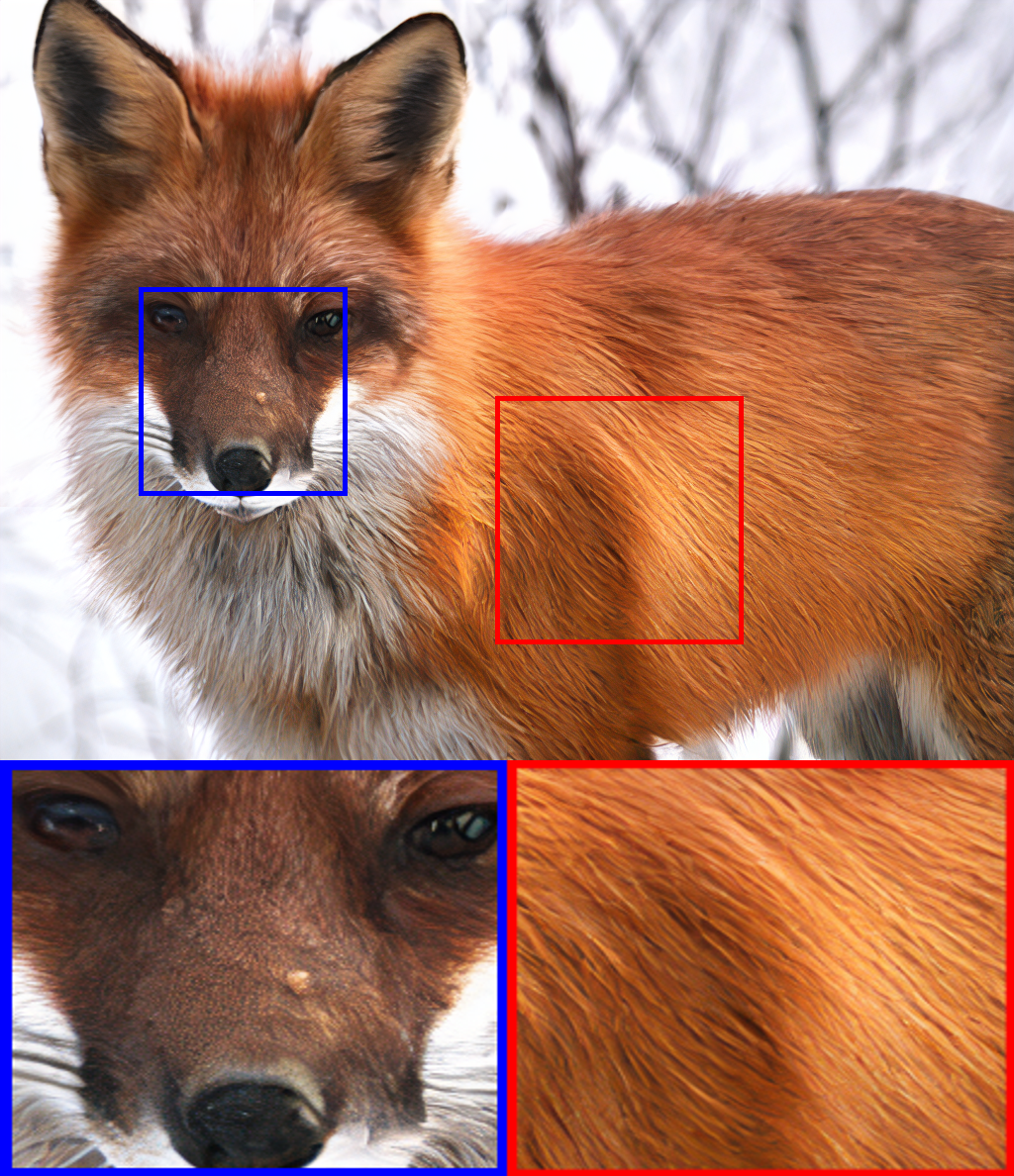
(b) Ours

Figure 12: LDM-SR super-resolution 4x upscaling result. In the regions highlighted by the blue and red boxes, Ours (DDIM 50 Step interval 3) (c) synthesizes more detailed textures effectively when compared to DDIM (b) with the same latency budget.

5.4.2 Memory Overhead

Table 2 presents the total amount of memory required for feature reusing. As shown in the table, our method can operate with a reasonable memory overhead. Additionally, for LDM-SR, there is a noticeable increase in memory overhead compared to the existing LDM. This is due to the memory being multiplied by the number of patches corresponding to the size of the super-resolution image. However, FRDiff is feasible on mid-grade GPUs.

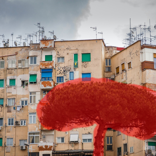
(a) Source Image

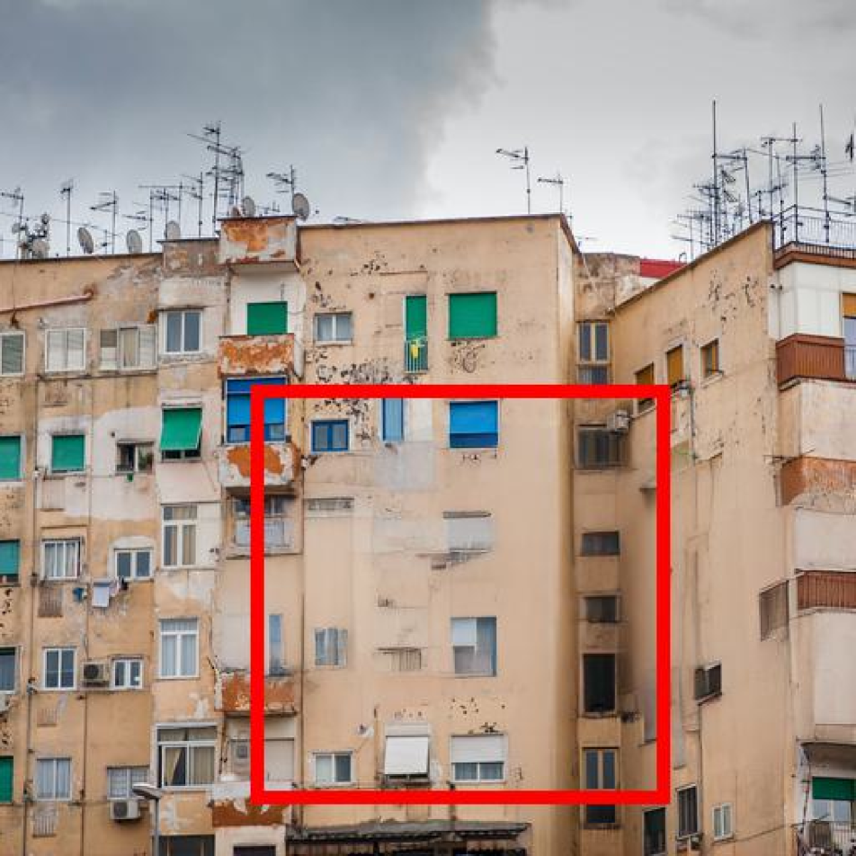
(b) DDIM 8 Step

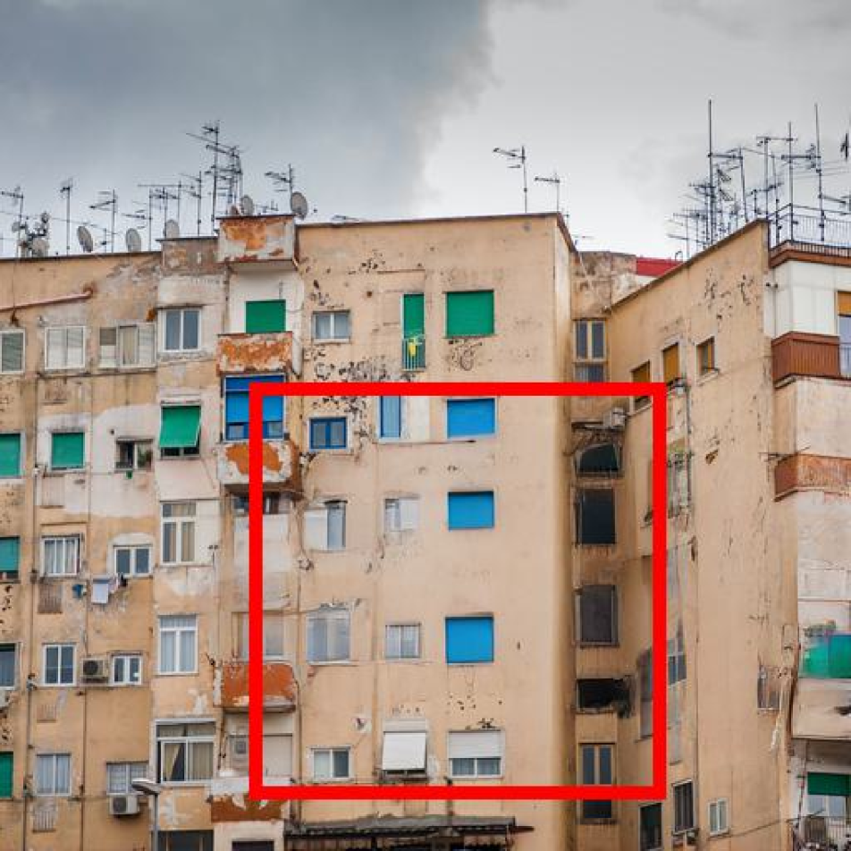
(c) Ours

Figure 13: LDM-Image Inpainting result of the source image (a). For comparison at the same latency, we compare DDIM 8 step (b) and Ours(DDIM 15 step interval 2) (c). As shown in the red box, Ours synthesizes the masked region reflecting the surrounding context more effectively than DDIM.

6 Discussion

In this section, we will discuss the drawbacks of our method and outline potential future work. While our method can be applied in a plug-and-play manner without being dependent on a specific ODE solver, it is not trivial to apply our method when the time step in score function evaluation is not continuously input. For instance, DPM-Solver++ [27] involves 2 or 3 non-consecutive score function evaluations to calculate a single score. In such cases, the performance of feature reusing can be degraded because of non-consecutive feature maps. For future work, we believe that considering the sensitivity of layers when applying feature reusing and reusing different layers over time may lead to improved performance. Additionally, performing an automatic search for time step intervals, mixing schedules, and skipping layer selection could be interesting areas for future research. Finally, instead of skipping the layer, exploring techniques like sparse convolution [9] or residual quantization [1] holds promise for future work.

7 Conclusion

In this paper, we propose FRDiff, a new Feature Reusing (FR) based zero-shot acceleration method for diffusion models. By leveraging strong temporal similarity arising from a iterative sampling process of the diffusion model, FRDiff can achieve up to 1.8x acceleration while maintaining high-quality output. Moreover, through a deep analysis of the generation process of the diffusion model, we introduce score mixing, a novel method that can leverage the strengths of both low NFE and FR. We validated our method across various task datasets, demonstrating that our approach achieves higher generation quality compared to existing zero-shot acceleration methods within the same latency budget.

Appendix

A Proof of Jump

In this section, we provide a proof that “Jump,” which indicates reusing the entire output score of the model for each consecutive step, is identical to reducing the NFE (Number of Function Evaluations).

First, we provide proof of this statement in the case of DDIM. The reverse process of DDIM at time $t$ is as follows:

$$x_{t-1}=\frac{\sqrt{\bar{\alpha}_{t-1}}}{\sqrt{\bar{\alpha}_{t}}}(x_{t}-\sqrt{1-\bar{\alpha}_{t}}\epsilon_{\theta}(x_{t}))\\ +\sqrt{1-\bar{\alpha}_{t-1}}\epsilon_{\theta}(x_{t})$$ (4)

The model predicts the score of the data $\epsilon_{\theta}(x_{t})$ at time t, and this score is used for denoising. Consider the case where the score obtained at time t ($\epsilon_{\theta}(x_{t})$) is used for the next time $t-1$, as in Eq. 5.

$$x_{t-2}=\frac{\sqrt{\bar{\alpha}_{t-2}}}{\sqrt{\bar{\alpha}_{t-1}}}(x_{t-1}-\sqrt{1-\bar{\alpha}_{t-1}}\epsilon_{\theta}(x_{t}))\\ +\sqrt{1-\bar{\alpha}_{t-2}}\epsilon_{\theta}(x_{t})$$ (5)

Then, combining Eq. 4 and Eq. 5, it can be expressed as:

$$x_{t-2}=\frac{\sqrt{\bar{\alpha}_{t-2}}}{\sqrt{\bar{\alpha}_{t-1}}}(\frac{\sqrt{\bar{\alpha}_{t-1}}}{\sqrt{\bar{\alpha}_{t}}}(x_{t}-\sqrt{1-\bar{\alpha}_{t}}\epsilon_{\theta}(x_{t}))$$

$$+\sqrt{1-\bar{\alpha}_{t-2}}\epsilon_{\theta}(x_{t})$$ (6)

Finally, the above equation can be represented as:

$$x_{t-2}=\frac{\sqrt{\bar{\alpha}_{t-2}}}{\sqrt{\bar{\alpha}_{t}}}(x_{t}-\sqrt{1-\bar{\alpha}_{t}}\epsilon_{\theta}(x_{t}))+\sqrt{1-\bar{\alpha}_{t-2}}\epsilon_{\theta}(x_{t})$$ (7)

This result corresponds to the reverse process over an interval of 2 at time $t$ in DDIM. Therefore, consistently using the output score of the model at time $t$ for subsequent jumps aligns with the goal of reducing the NFE.

B Details on Score Mixing

In this section, we provide a detailed explanation of Score Mixing. As mentioned in main paper, we propose to mix score(output of unet) generated by FR and preceding time step with predefined scheduling function $\lambda(t)$. The pseudo code of this algorithm is shown in Algorithm 1. The $Update(\cdot)$ in line 13 is equal to Eq. 4.

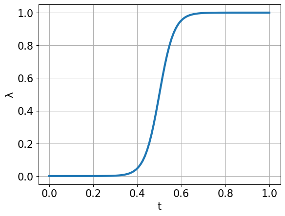
(a) Sigmoid

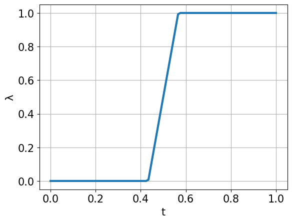
(b) Hard Sigmoid

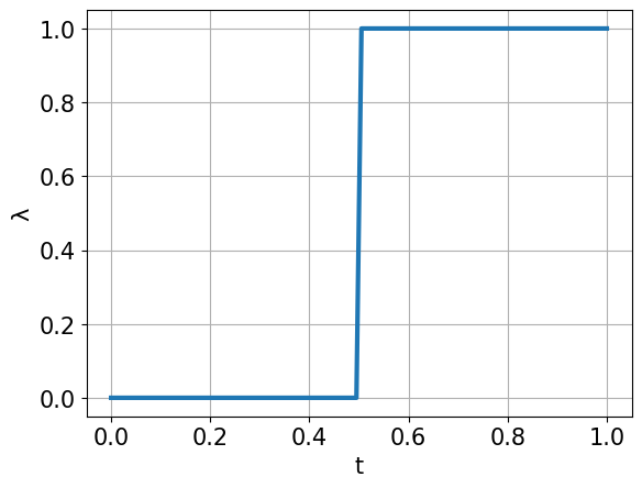
(c) Step Function

Figure 14: 3 types of lambda Function $\lambda(t)$ we considered.

Besides, we design 3 types of $\lambda(t)$ to experiment effect of score mixing and trade-off between this functions. These functions are described in Fig. 14 and defined as follows :

Sigmoid function is defined as follows:

$$\lambda(t)=\frac{1}{1+e^{-\tau(t-b)}}$$ (8)

Hard sigmoid function is defined as follows:

$$\lambda(t)=max(0,min(1,((t-b)*\tau+2)/4))$$ (9)

Step function is defined as follows:

$$\lambda(t)=\begin{cases}0&\text{if }x<b\\ 1&\text{if }x\geq b\end{cases}$$ (10)

where the temperature parameter $\tau$ affectes the slope of the sigmoid function and $b$ act as a bias term, determining the transition point of jump and FR. By considering both generation quality and latency, we decided to use Hard-Sigmoid funtion with $\tau=30,b=0.5$ in every experiment. The ablation study on the lambda function is presented in the main paper.

Input: $x_{T}\sim N(0,I)$, T, interval

Output: Generated sample $x_{0}$

for t = 0, 1, …, T do

       if t % interval = 0 then

             $\epsilon_{t}$ $\leftarrow$ $\epsilon_{\theta}$($x_{t}$, $t$)

             $\epsilon_{keyframe}$ $\leftarrow$ $\epsilon_{t}$

            

      else

            

            $\lambda_{t}$ $\leftarrow$ $\lambda(t/T)$

            

            if $\lambda_{t}$ = $0$ then

                   $\epsilon_{t}$ $\leftarrow$ $\epsilon_{keyframe}$

                  

            else

                   $\epsilon_{t}$ $\leftarrow$ $\lambda_{t}$ $\epsilon_{\theta}$($x_{t}$, $t$)_FR + (1-$\lambda_{t}$)$\epsilon_{keyframe}$

                  

            

      

      $x_{t-1}$ $\leftarrow$ Update($x_{t}$, ${\epsilon}_{t}$)

      

return $x_{0}$

Algorithm 1 Score Mixing

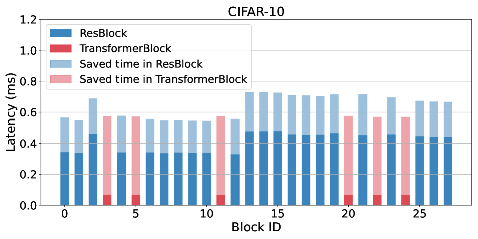
(a) CIFAR-10

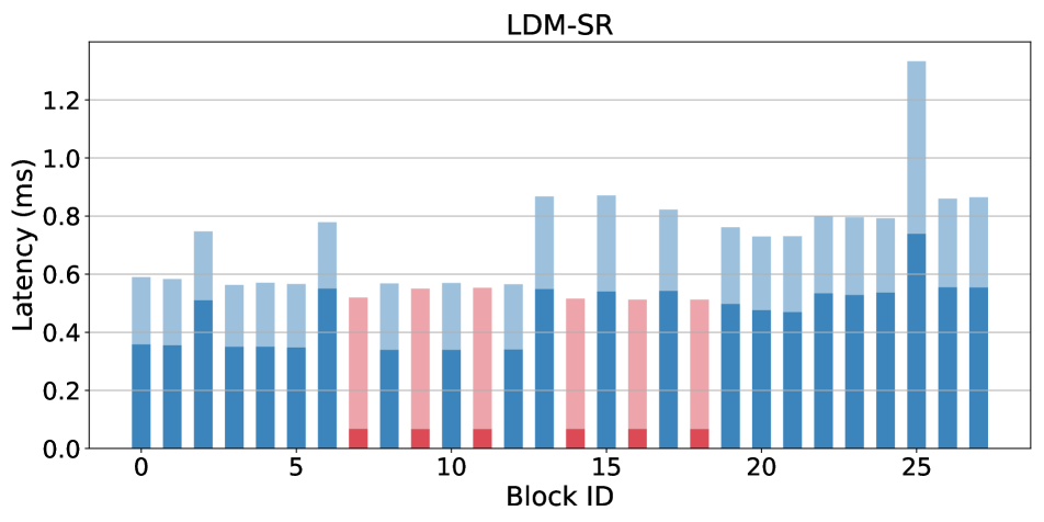
(b) LDM-SR

Figure 15: Skippable latency with Feature Reuse in CIFAR-10, LDM-SR

C Skippable Latency

In this section, we provide the latency benefits of feature reuse (FR) for more models, CIFAR-10, and LDM-SR in Fig.15. These models have more ResBlocks, which only reuse the feature map before the time embed, compared to Attention Blocks, which reuse every operation before the residual. Therefore, when there are a significant number of ResBlocks than Attention Blocks, the acceleration obtained through FR may be limited.

D Power Spectral Density Analysis

In this section, we provide a Power Spectral Density (PSD) analysis of random images generated from LDM-CelebA-HQ and Stable Diffusion in Fig.17, 18. All results are measured with 50 steps of NFE, and the skip interval is indicated by the color gradient from blue to yellow. As the skip interval increases, Jump shows a significant decrease in high-frequency components, while FR fails to maintain low-frequency components. Besides, our Mix preserves both frequency components well.

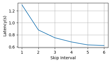
(a) LDM-CelebA

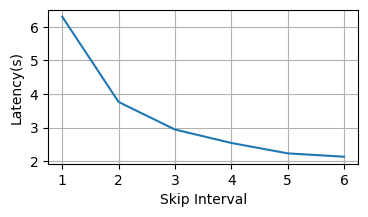
(b) Stable Diffusion

Figure 16: Skip Interval vs Latency.

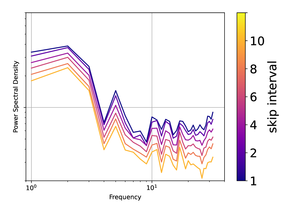
(a) Jump

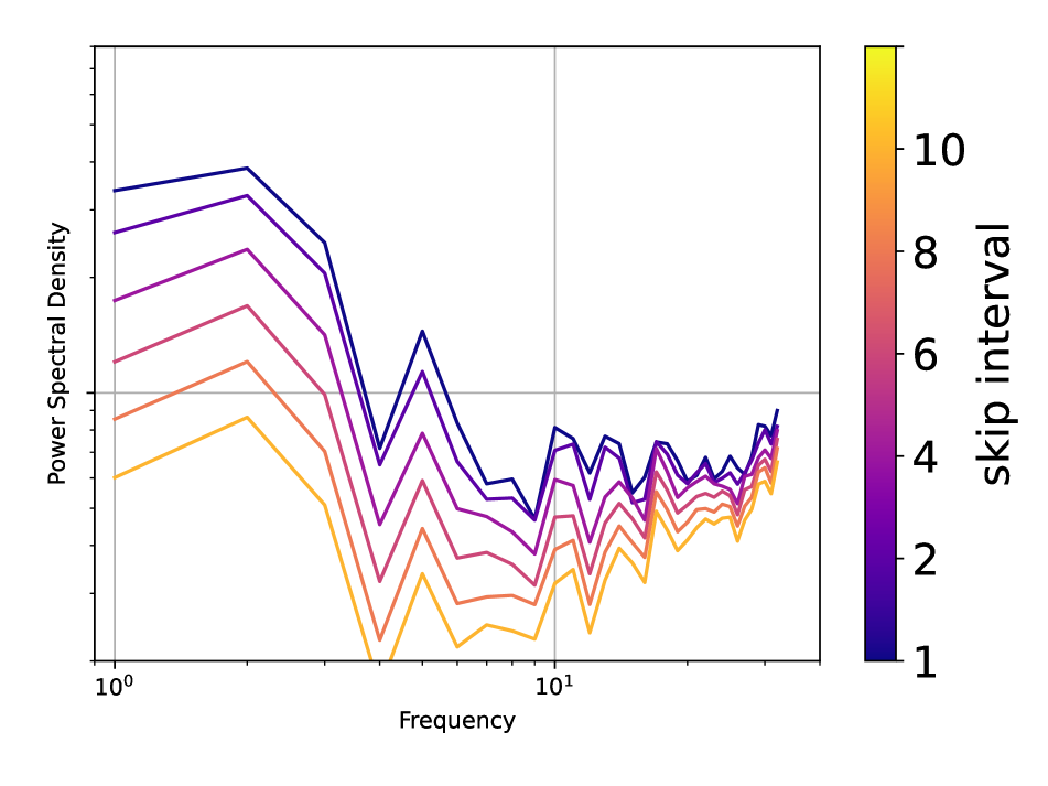
(b) FR

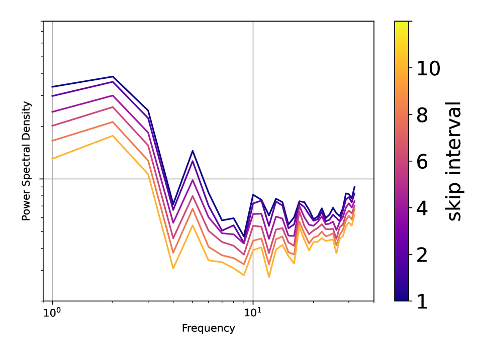
(c) Mix

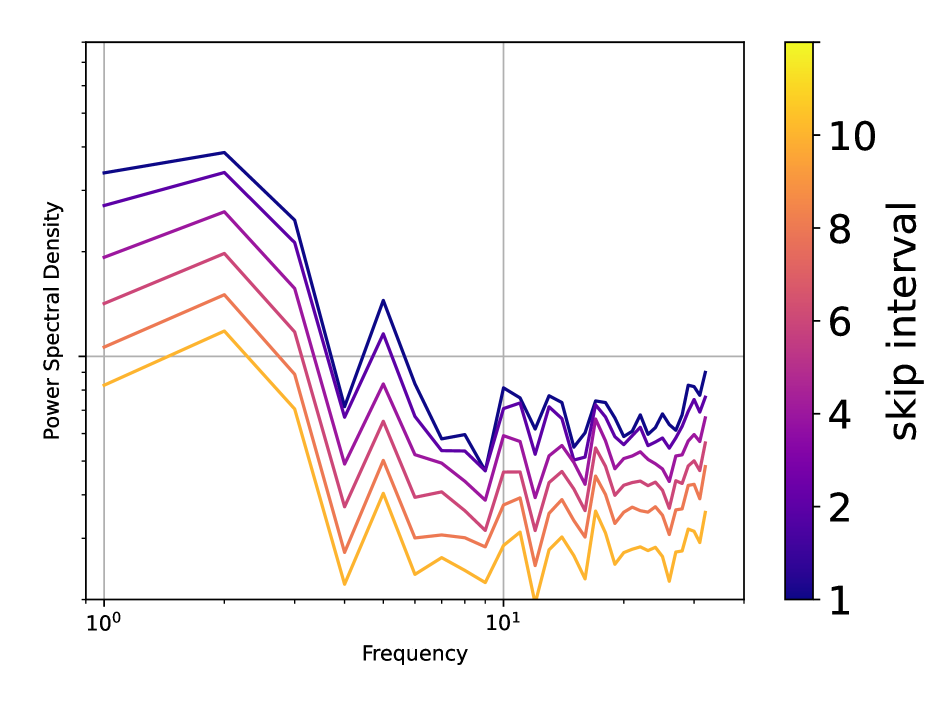
(d) Mix-R

Figure 17: Power Spectral Density(PSD) of Random Sampled CelebA-HQ generated results

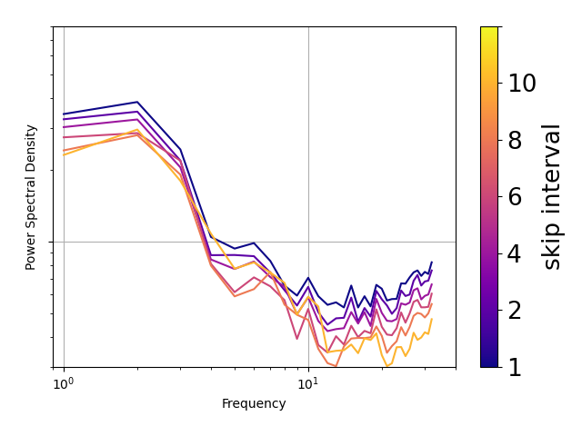
(a) Jump

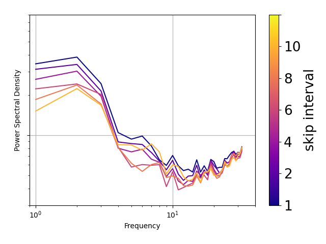
(b) FR

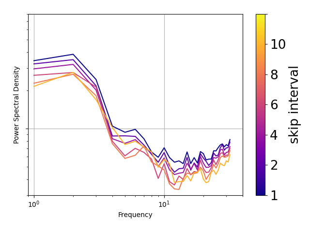
(c) Mix

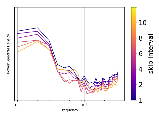
(d) Mix-R

Figure 18: Power Spectral Density(PSD) of Random Sampled Stable Diffusion generated results

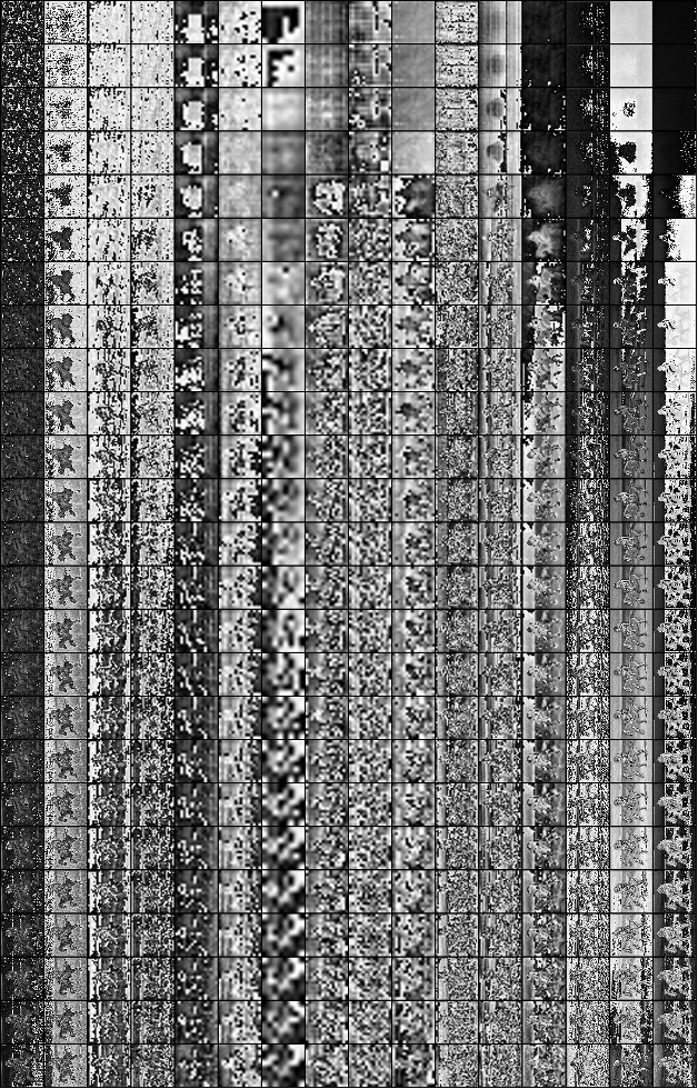
Figure 19: Visualization of feature map in Transformer Block. The X-axis represents the Block ID, and the Y-axis represents the time step.

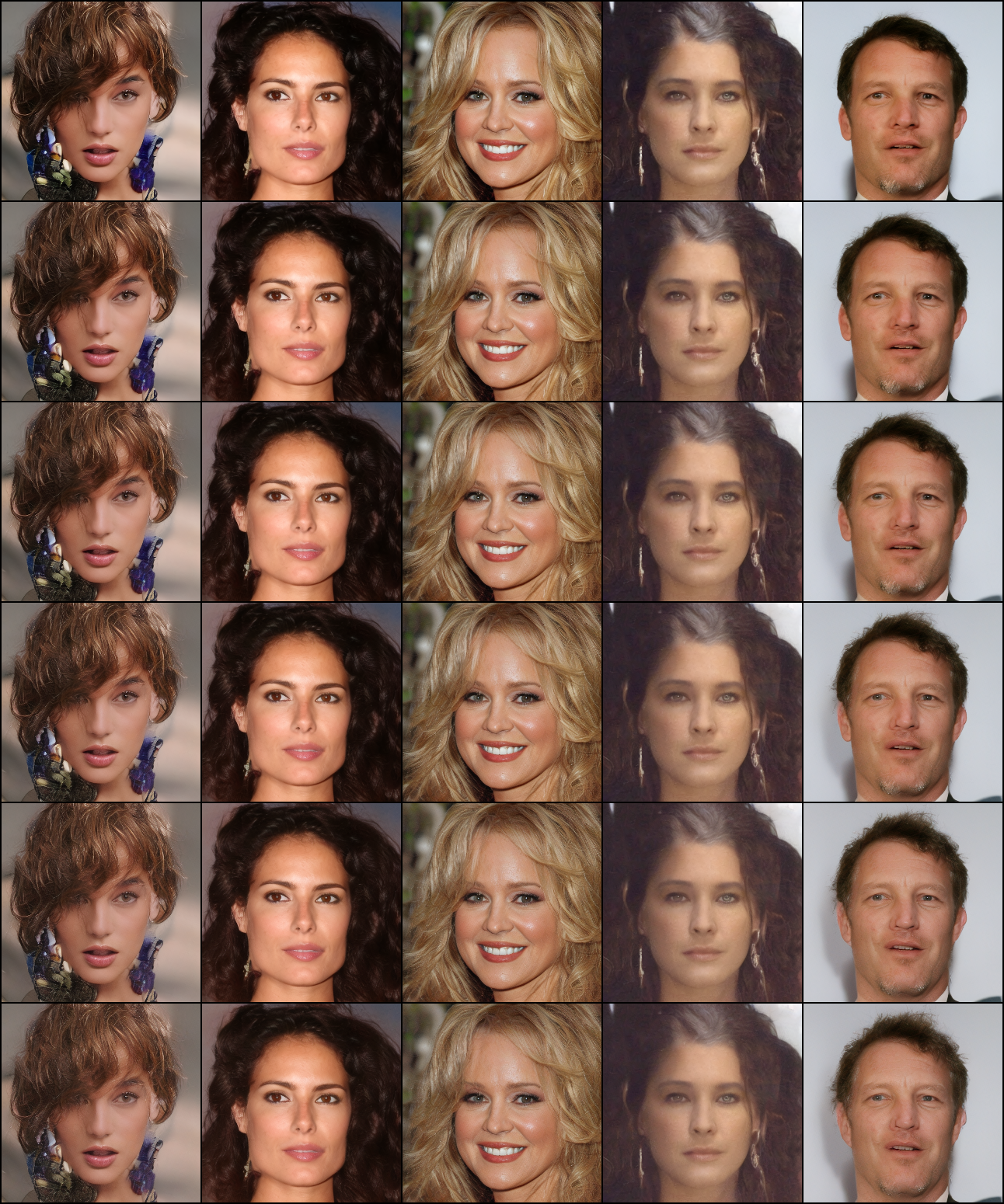
Figure 20: DDIM 50 step CelebA-HQ Random Sampling result with FRDiff. Each row represents the generated result with increasing skip intervals, where the intervals are 1, 2, 3, 4, 5, 6.

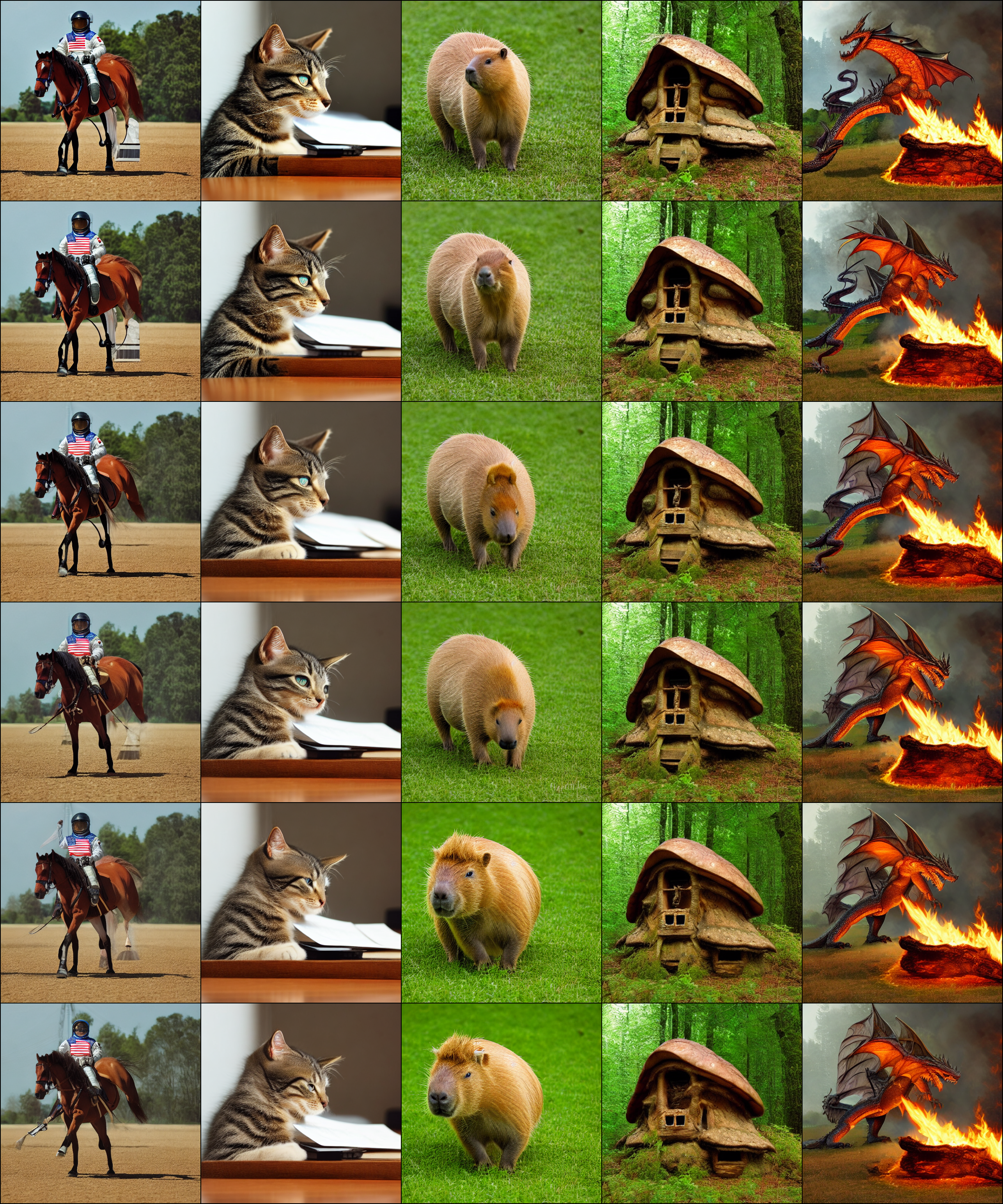
Figure 21: DDIM 50 step Stable Diffusion Random Sampling result with FRDiff. Each row represents the generated result with increasing skip intervals, where the intervals are 1, 2, 3, 4, 5, 6.

E Feature Similarity Visualization

To illustrate the temporal redundancy in feature maps over time, Fig. 19 provides visualizations of feature maps during sampling in Stable Diffusion. These feature maps are collected from the first channel of the output feature map of the Transformer Block over a 25-step sampling period. As evident in the visualization, feature maps exhibit strong similarity across all blocks for adjacent time steps, indicating the presence of temporal redundancy. These results robustly support the efficiency of feature reuse.

F Additional Sampling Results

F.0.1 Text-to-Image

In this section, we present additional sampling results obtained using FRDiff. Fig. 20 and  21 depict the results of unconditional generation (CelebA-HQ) and text-to-image generation (Stable Diffusion), respectively, when gradually increasing the skip interval. These figures shows that FR has negligible image degradation except in situations where the interval is too large. Additionally, in Fig. 16, we plotted the measured latency for the FRDiff-applied DDIM 50 steps of each model by increasing the skip interval. As shown in the figure, the latency shows saturation when the interval is around 6. However, in other cases, the latency decreases almost linearly. These results indicate that we can achieve sufficient acceleration while preventing degradation in generation quality by using FRDiff.

F.0.2 Super Resolution and Image Inpainting

In Fig.  22 and  23, we compare DDIM and FRDiff for super-resolution and image inpainting under the same latency budget. The super-resolution results are generated through 4x upscaling of 256x256 images from the ImageNet validation set. To ensure a fair latency comparison, the results utilize DDIM with 30 steps and FRDiff with 50 steps at interval 3. The image inpainting results use the MS-COCO validation set, comparing DDIM with 8 steps and FRDiff with 15 steps, with an interval of 2. All provided images are randomly generated results without any cherry-picking.

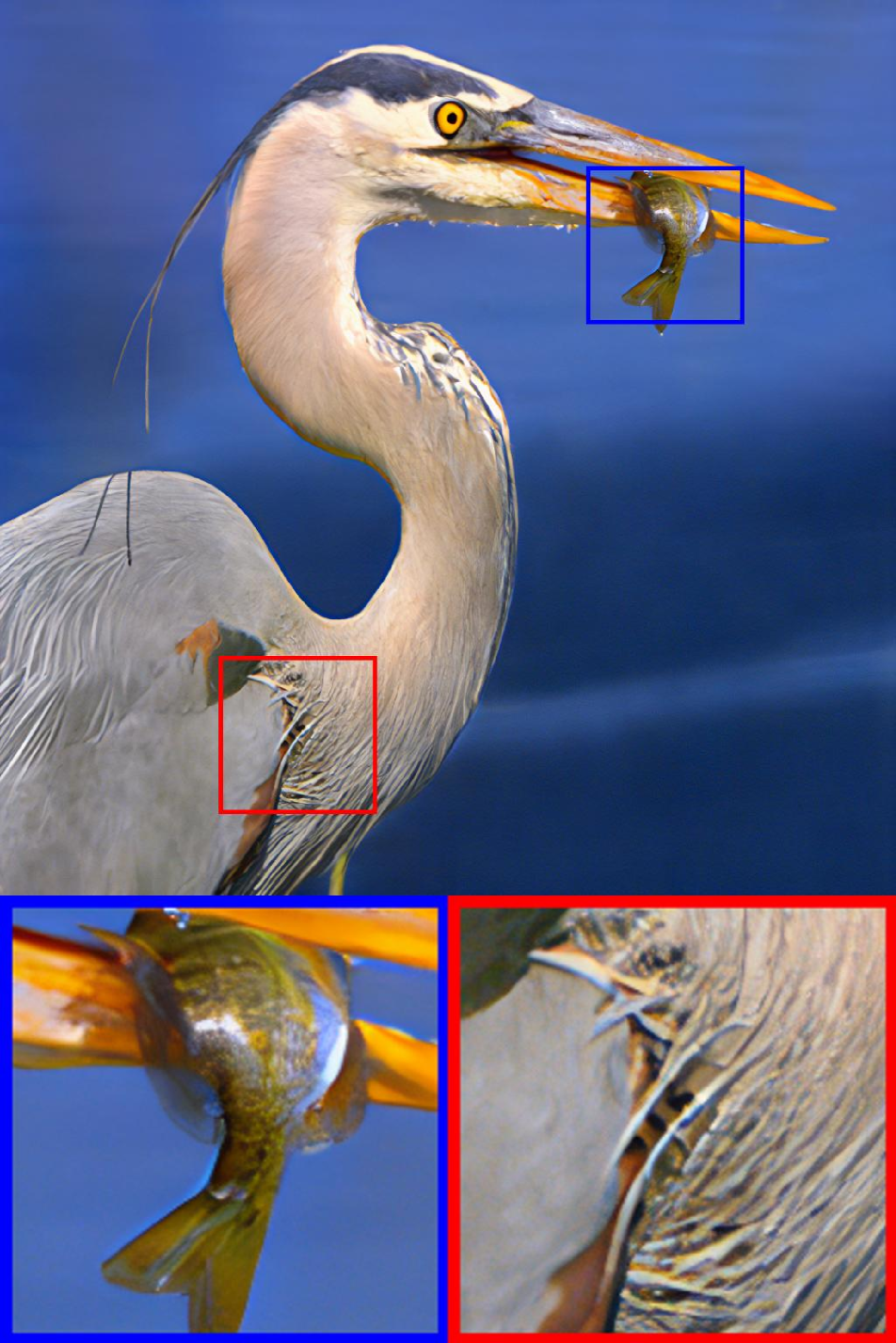
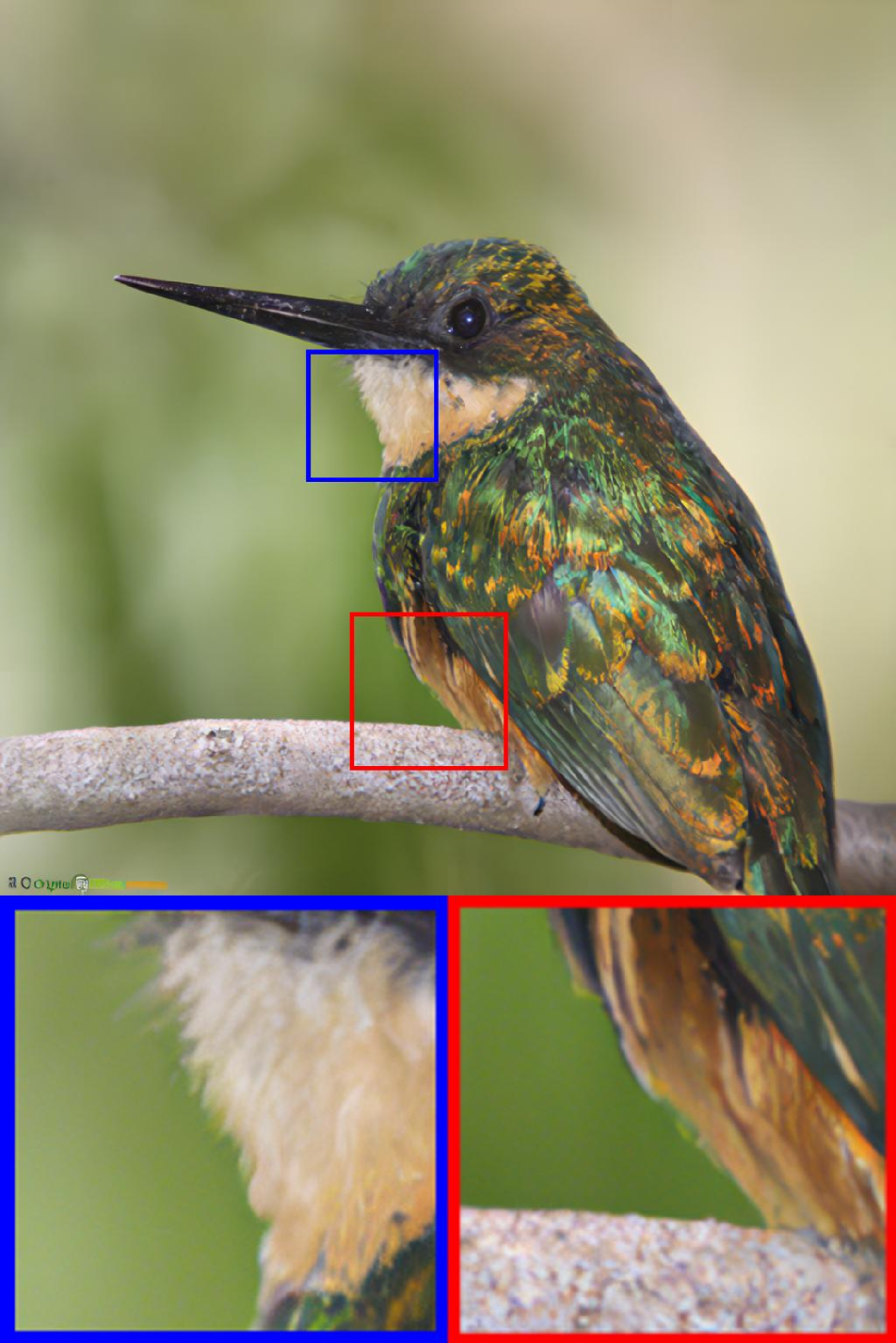
(a) DDIM

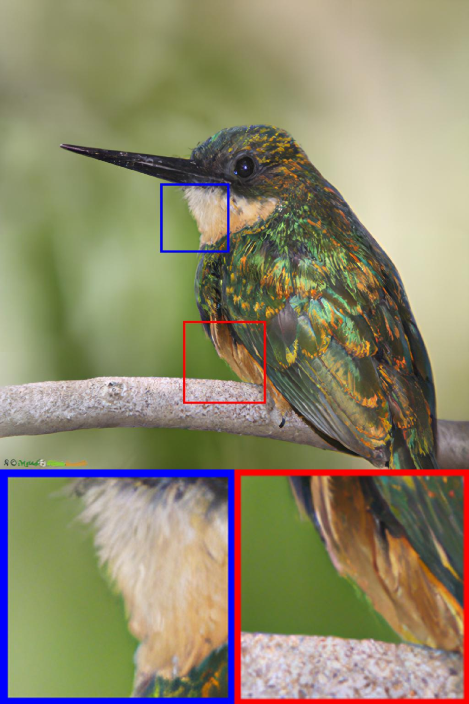
(b) Ours

Figure 22: Super-resolution Result on ImageNet-Validation set

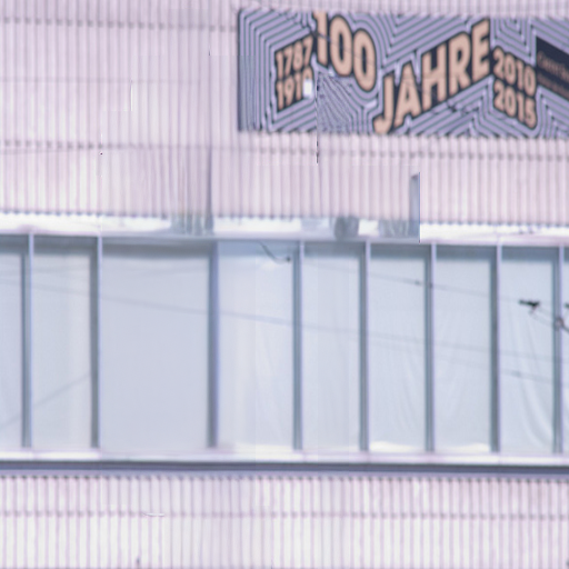
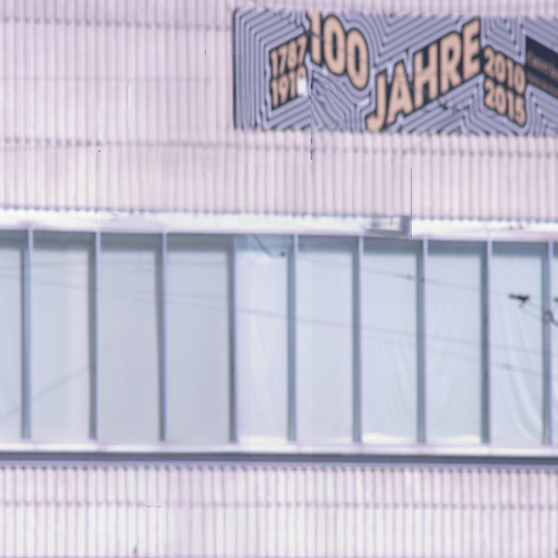
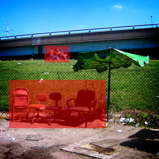
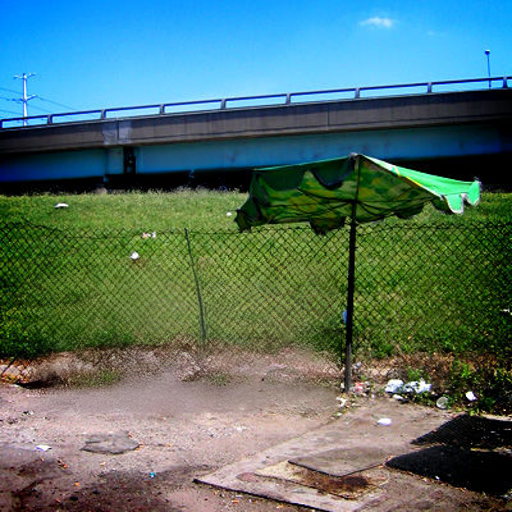
(a) Source Image

(b) DDIM

(c) Ours

Figure 23: Image Inpainting Result

References

- Abati et al. [2023] Davide Abati, Haitam Ben Yahia, Markus Nagel, and Amirhossein Habibian. Resq: Residual quantization for video perception. In Proceedings of the IEEE/CVF International Conference on Computer Vision, pages 17119–17129, 2023.
- Bansal et al. [2023] Arpit Bansal, Hong-Min Chu, Avi Schwarzschild, Soumyadip Sengupta, Micah Goldblum, Jonas Geiping, and Tom Goldstein. Universal guidance for diffusion models. In CVPR, pages 843–852, 2023.
- Bolya and Hoffman [2023] Daniel Bolya and Judy Hoffman. Token merging for fast stable diffusion. In Proceedings of the IEEE/CVF Conference on Computer Vision and Pattern Recognition, pages 4598–4602, 2023.
- Brooks et al. [2023] Tim Brooks, Aleksander Holynski, and Alexei A Efros. Instructpix2pix: Learning to follow image editing instructions. In CVPR, pages 18392–18402, 2023.
- Choi et al. [2022] Jooyoung Choi, Jungbeom Lee, Chaehun Shin, Sungwon Kim, Hyunwoo Kim, and Sungroh Yoon. Perception prioritized training of diffusion models. In Proceedings of the IEEE/CVF Conference on Computer Vision and Pattern Recognition, pages 11472–11481, 2022.
- Deng et al. [2009] Jia Deng, Wei Dong, Richard Socher, Li-Jia Li, Kai Li, and Li Fei-Fei. Imagenet: A large-scale hierarchical image database. In 2009 IEEE conference on computer vision and pattern recognition, pages 248–255. Ieee, 2009.
- Fang et al. [2023] Gongfan Fang, Xinyin Ma, and Xinchao Wang. Structural pruning for diffusion models. arXiv preprint arXiv:2305.10924, 2023.
- Goodfellow et al. [2020] Ian Goodfellow, Jean Pouget-Abadie, Mehdi Mirza, Bing Xu, David Warde-Farley, Sherjil Ozair, Aaron Courville, and Yoshua Bengio. Generative adversarial networks. Communications of the ACM, 63(11):139–144, 2020.
- Habibian et al. [2021] Amirhossein Habibian, Davide Abati, Taco S Cohen, and Babak Ehteshami Bejnordi. Skip-convolutions for efficient video processing. In Proceedings of the IEEE/CVF Conference on Computer Vision and Pattern Recognition, pages 2695–2704, 2021.
- Ham et al. [2023] Cusuh Ham, James Hays, Jingwan Lu, Krishna Kumar Singh, Zhifei Zhang, and Tobias Hinz. Modulating pretrained diffusion models for multimodal image synthesis. SIGGRAPH Conference Proceedings, 2023.
- He et al. [2016] Kaiming He, Xiangyu Zhang, Shaoqing Ren, and Jian Sun. Deep residual learning for image recognition. In Proceedings of the IEEE conference on computer vision and pattern recognition, pages 770–778, 2016.
- Hertz et al. [2023] Amir Hertz, Kfir Aberman, and Daniel Cohen-Or. Delta denoising score. In ICCV, pages 2328–2337, 2023.
- Heusel et al. [2017] Martin Heusel, Hubert Ramsauer, Thomas Unterthiner, Bernhard Nessler, and Sepp Hochreiter. Gans trained by a two time-scale update rule converge to a local nash equilibrium. Advances in neural information processing systems, 30, 2017.
- Ho and Salimans [2022] Jonathan Ho and Tim Salimans. Classifier-free diffusion guidance. arXiv preprint arXiv:2207.12598, 2022.
- Ho et al. [2020] Jonathan Ho, Ajay Jain, and Pieter Abbeel. Denoising diffusion probabilistic models. Advances in neural information processing systems, 33:6840–6851, 2020.
- Karras et al. [2017] Tero Karras, Timo Aila, Samuli Laine, and Jaakko Lehtinen. Progressive growing of gans for improved quality, stability, and variation. arXiv preprint arXiv:1710.10196, 2017.
- Karras et al. [2022] Tero Karras, Miika Aittala, Timo Aila, and Samuli Laine. Elucidating the design space of diffusion-based generative models. Advances in Neural Information Processing Systems, 35:26565–26577, 2022.
- Kim et al. [2023] Bo-Kyeong Kim, Hyoung-Kyu Song, Thibault Castells, and Shinkook Choi. On architectural compression of text-to-image diffusion models. arXiv preprint arXiv:2305.15798, 2023.
- Kingma and Welling [2013] Diederik P Kingma and Max Welling. Auto-encoding variational bayes. arXiv preprint arXiv:1312.6114, 2013.
- Krizhevsky et al. [2009] Alex Krizhevsky, Geoffrey Hinton, et al. Learning multiple layers of features from tiny images. 2009.
- Li et al. [2023] Xiuyu Li, Yijiang Liu, Long Lian, Huanrui Yang, Zhen Dong, Daniel Kang, Shanghang Zhang, and Kurt Keutzer. Q-diffusion: Quantizing diffusion models. In Proceedings of the IEEE/CVF International Conference on Computer Vision, pages 17535–17545, 2023.
- Lin et al. [2014] Tsung-Yi Lin, Michael Maire, Serge Belongie, James Hays, Pietro Perona, Deva Ramanan, Piotr Dollár, and C Lawrence Zitnick. Microsoft coco: Common objects in context. In Computer Vision–ECCV 2014: 13th European Conference, Zurich, Switzerland, September 6-12, 2014, Proceedings, Part V 13, pages 740–755. Springer, 2014.
- Lin et al. [2023] Xinqi Lin, Jingwen He, Ziyan Chen, Zhaoyang Lyu, Ben Fei, Bo Dai, Wanli Ouyang, Yu Qiao, and Chao Dong. Diffbir: Towards blind image restoration with generative diffusion prior. arXiv preprint arXiv:2308.15070, 2023.
- Liu et al. [2022a] Luping Liu, Yi Ren, Zhijie Lin, and Zhou Zhao. Pseudo numerical methods for diffusion models on manifolds. arXiv preprint arXiv:2202.09778, 2022a.
- Liu et al. [2022b] Xingchao Liu, Chengyue Gong, and Qiang Liu. Flow straight and fast: Learning to generate and transfer data with rectified flow. arXiv preprint arXiv:2209.03003, 2022b.
- Lu et al. [2022a] Cheng Lu, Yuhao Zhou, Fan Bao, Jianfei Chen, Chongxuan Li, and Jun Zhu. Dpm-solver: A fast ode solver for diffusion probabilistic model sampling in around 10 steps. Advances in Neural Information Processing Systems, 35:5775–5787, 2022a.
- Lu et al. [2022b] Cheng Lu, Yuhao Zhou, Fan Bao, Jianfei Chen, Chongxuan Li, and Jun Zhu. Dpm-solver++: Fast solver for guided sampling of diffusion probabilistic models. arXiv preprint arXiv:2211.01095, 2022b.
- Luo et al. [2023] Simian Luo, Yiqin Tan, Longbo Huang, Jian Li, and Hang Zhao. Latent consistency models: Synthesizing high-resolution images with few-step inference. arXiv preprint arXiv:2310.04378, 2023.
- Ma et al. [2022] Hengyuan Ma, Li Zhang, Xiatian Zhu, and Jianfeng Feng. Accelerating score-based generative models with preconditioned diffusion sampling. In European Conference on Computer Vision, pages 1–16. Springer, 2022.
- Meng et al. [2023] Chenlin Meng, Robin Rombach, Ruiqi Gao, Diederik Kingma, Stefano Ermon, Jonathan Ho, and Tim Salimans. On distillation of guided diffusion models. In Proceedings of the IEEE/CVF Conference on Computer Vision and Pattern Recognition, pages 14297–14306, 2023.
- Mou et al. [2023] Chong Mou, Xintao Wang, Liangbin Xie, Jian Zhang, Zhongang Qi, Ying Shan, and Xiaohu Qie. T2i-adapter: Learning adapters to dig out more controllable ability for text-to-image diffusion models. arXiv preprint arXiv:2302.08453, 2023.
- Paszke et al. [2019] Adam Paszke, Sam Gross, Francisco Massa, Adam Lerer, James Bradbury, Gregory Chanan, Trevor Killeen, Zeming Lin, Natalia Gimelshein, Luca Antiga, et al. Pytorch: An imperative style, high-performance deep learning library. Advances in neural information processing systems, 32, 2019.
- Podell et al. [2023] Dustin Podell, Zion English, Kyle Lacey, Andreas Blattmann, Tim Dockhorn, Jonas Müller, Joe Penna, and Robin Rombach. Sdxl: Improving latent diffusion models for high-resolution image synthesis. arXiv preprint arXiv:2307.01952, 2023.
- Ramesh et al. [2021] Aditya Ramesh, Mikhail Pavlov, Gabriel Goh, Scott Gray, Chelsea Voss, Alec Radford, Mark Chen, and Ilya Sutskever. Zero-shot text-to-image generation. In International Conference on Machine Learning, pages 8821–8831. PMLR, 2021.
- Ravi et al. [2023] Hareesh Ravi, Sachin Kelkar, Midhun Harikumar, and Ajinkya Kale. Preditor: Text guided image editing with diffusion prior. arXiv preprint arXiv:2302.07979, 2023.
- Rombach et al. [2022] Robin Rombach, Andreas Blattmann, Dominik Lorenz, Patrick Esser, and Björn Ommer. High-resolution image synthesis with latent diffusion models. In CVPR, pages 10684–10695, 2022.
- Ronneberger et al. [2015] Olaf Ronneberger, Philipp Fischer, and Thomas Brox. U-net: Convolutional networks for biomedical image segmentation. In Medical Image Computing and Computer-Assisted Intervention–MICCAI 2015: 18th International Conference, Munich, Germany, October 5-9, 2015, Proceedings, Part III 18, pages 234–241. Springer, 2015.
- Saharia et al. [2022] Chitwan Saharia, William Chan, Saurabh Saxena, Lala Li, Jay Whang, Emily L Denton, Kamyar Ghasemipour, Raphael Gontijo Lopes, Burcu Karagol Ayan, Tim Salimans, et al. Photorealistic text-to-image diffusion models with deep language understanding. NeurIPS, 35:36479–36494, 2022.
- Salimans and Ho [2022] Tim Salimans and Jonathan Ho. Progressive distillation for fast sampling of diffusion models. arXiv preprint arXiv:2202.00512, 2022.
- Schuhmann et al. [2022] Christoph Schuhmann, Romain Beaumont, Richard Vencu, Cade W Gordon, Ross Wightman, Mehdi Cherti, Theo Coombes, Aarush Katta, Clayton Mullis, Mitchell Wortsman, et al. Laion-5b: An open large-scale dataset for training next generation image-text models. In Thirty-sixth Conference on Neural Information Processing Systems Datasets and Benchmarks Track, 2022.
- So et al. [2023] Junhyuk So, Jungwon Lee, Daehyun Ahn, Hyungjun Kim, and Eunhyeok Park. Temporal dynamic quantization for diffusion models. arXiv preprint arXiv:2306.02316, 2023.
- Sohl-Dickstein et al. [2015] Jascha Sohl-Dickstein, Eric Weiss, Niru Maheswaranathan, and Surya Ganguli. Deep unsupervised learning using nonequilibrium thermodynamics. In International conference on machine learning, pages 2256–2265. PMLR, 2015.
- Song et al. [2020a] Jiaming Song, Chenlin Meng, and Stefano Ermon. Denoising diffusion implicit models. arXiv preprint arXiv:2010.02502, 2020a.
- Song et al. [2020b] Yang Song, Jascha Sohl-Dickstein, Diederik P Kingma, Abhishek Kumar, Stefano Ermon, and Ben Poole. Score-based generative modeling through stochastic differential equations. arXiv preprint arXiv:2011.13456, 2020b.
- Song et al. [2023] Yang Song, Prafulla Dhariwal, Mark Chen, and Ilya Sutskever. Consistency models. 2023.
- Tumanyan et al. [2023] Narek Tumanyan, Michal Geyer, Shai Bagon, and Tali Dekel. Plug-and-play diffusion features for text-driven image-to-image translation. In CVPR, pages 1921–1930, 2023.
- Vaswani et al. [2017] Ashish Vaswani, Noam Shazeer, Niki Parmar, Jakob Uszkoreit, Llion Jones, Aidan N Gomez, Łukasz Kaiser, and Illia Polosukhin. Attention is all you need. Advances in neural information processing systems, 30, 2017.
- Wang et al. [2023a] Jianyi Wang, Zongsheng Yue, Shangchen Zhou, Kelvin CK Chan, and Chen Change Loy. Exploiting diffusion prior for real-world image super-resolution. arXiv preprint arXiv:2305.07015, 2023a.
- Wang et al. [2023b] Qian Wang, Biao Zhang, Michael Birsak, and Peter Wonka. Mdp: A generalized framework for text-guided image editing by manipulating the diffusion path. arXiv preprint arXiv:2303.16765, 2023b.
- Xie et al. [2023] Jinheng Xie, Yuexiang Li, Yawen Huang, Haozhe Liu, Wentian Zhang, Yefeng Zheng, and Mike Zheng Shou. Boxdiff: Text-to-image synthesis with training-free box-constrained diffusion. In ICCV, pages 7452–7461, 2023.
- Xu et al. [2023] Yilun Xu, Mingyang Deng, Xiang Cheng, Yonglong Tian, Ziming Liu, and Tommi Jaakkola. Restart sampling for improving generative processes. arXiv preprint arXiv:2306.14878, 2023.
- Yang et al. [2023a] Binbin Yang, Yi Luo, Ziliang Chen, Guangrun Wang, Xiaodan Liang, and Liang Lin. Law-diffusion: Complex scene generation by diffusion with layouts. In Proceedings of the IEEE/CVF International Conference on Computer Vision, pages 22669–22679, 2023a.
- Yang et al. [2023b] Xingyi Yang, Daquan Zhou, Jiashi Feng, and Xinchao Wang. Diffusion probabilistic model made slim. In Proceedings of the IEEE/CVF Conference on Computer Vision and Pattern Recognition, pages 22552–22562, 2023b.
- Yu et al. [2023] Jiwen Yu, Yinhuai Wang, Chen Zhao, Bernard Ghanem, and Jian Zhang. Freedom: Training-free energy-guided conditional diffusion model. ICCV, 2023.
- Zhang et al. [2023] Lvmin Zhang, Anyi Rao, and Maneesh Agrawala. Adding conditional control to text-to-image diffusion models. In CVPR, pages 3836–3847, 2023.
- Zhang et al. [2022] Qinsheng Zhang, Molei Tao, and Yongxin Chen. gddim: Generalized denoising diffusion implicit models. arXiv preprint arXiv:2206.05564, 2022.