Abstract

The physics of primordial black holes can be affected by the non-Gaussian statistics of the density fluctuations that generate them. Therefore, it is important to have good theoretical control of the higher-order correlation functions for primordial curvature perturbations. By working at leading order in a $1/|\eta|$ expansion, we analytically determine the bispectrum of curvature fluctuations for single field inflationary scenarios producing primordial black holes. The bispectrum has a rich scale and shape dependence, and its features depend on the dynamics of the would-be decaying mode. We apply our analytical results to study gravitational waves induced at second order by enhanced curvature fluctuations. Their statistical properties are derived in terms of convolution integrals over wide momentum ranges, and they are sensitive on the scale and shape dependence of the curvature bispectrum we analytically computed.

1 Introduction and Conclusions

The lack of direct detection of particle dark matter motivates the study of primordial black holes (PBH) [1, 2, 3, 4] as dark matter candidate. Primordial black holes are formed by the collapse of density fluctuations produced during cosmic inflation. See e.g. [5, 6, 7, 8, 9, 10, 11] for reviews. In order for producing PBH, the size of the inflationary curvature fluctuation spectrum should increase by several orders of magnitude from large towards small scales. This condition can be achieved by models of inflation violating the standard slowroll conditions, at least during a short epoch within the inflationary process (see e.g. [12] for an introduction to standard slowroll inflation). In the simplest PBH-forming scenarios, while the parameter $\epsilon$ remains small, the absolute value of the parameter $\eta$ become well larger than one during a short range $\Delta N_{\rm NSR}$ of inflationary e-folds. Typically, since we can not rely on a perturbative slowroll expansion, the analysis of such non slowroll models requires the use of numerical techniques – although interesting specific scenarios exist, which are amenable of analytic investigation: see e.g. [13, 14, 15, 16, 17, 18, 19, 20, 21].

The work [22] proposes a new perturbative framework based on an expansion in inverse powers of a small parameter $1/|\eta|$. Let us assume that the quantity $|\eta|$ is very large. At the same time, the duration of non slowroll phase $\Delta N_{\rm NSR}$ is infinitesimally small, while the value for the product $|\eta|\,\Delta N_{\rm NSR}$ is kept finite. Cosmological observables based on correlators of curvature perturbations can be then calculated analytically, leading to formulas organized in a $1/|\eta|$ expansion. There is hope that the results of these calculations share general features with the statistics of curvature perturbations computed within more general (and realistic) families of PBH-forming scenarios, characterised by finite values of $|\eta|$. There are interesting analogies with other approaches developed within quantum field theory, as ’t Hooft $1/N$ expansion [23]. In such a framework, the large $N$ limit of $SU(N)$ gauge theories is able to shed light on the properties of quantum chromodynamics, characterized by $N=3$ (see e.g. [24] for a pedagogical introduction to the subject).

The scope of this work is to analyze more systematically features of non-Gaussian correlators using the large $|\eta|$ approach to single field inflation, going beyond the investigations started in [22]. Primordial Non-Gaussianities can be generated in scenarios producing PBH in inflation, see e.g. [25, 26, 27, 28, 29, 30]. They play an important role in the physics of primordial black holes, since the formation of compact objects depends on the statistics of curvature fluctuations and their probability distribution function, see e.g. [31, 32, 33, 34, 35, 36, 37, 38, 39, 40, 41, 42, 43, 44, 45, 46, 47, 48, 49, 50, 51, 52, 53, 54, 55]. It is then important to have a good analytical control of the properties of the primordial bispectrum in PBH models. After a brief review of the motivations and tools for carrying on a $1/|\eta|$ expansion – see section 2, based on [22] – we focus in section 3 in computing the bispectrum. We discuss the properties of the three point functions of curvature perturbations. Interestingly, our approach allows us to determine the leading contributions of the third order interactions Hamiltonian, and leads us to analytically compute the bispectrum at leading order in a $1/|\eta|$ expansion. The result depends on a single free parameter, which controls the enhancement of the spectrum from large towards small scales. We nevertheless find a very rich scale and shape dependence, which we analyze in detail. Depending on the scale, the bispectrum can be enhanced on an equilateral shape, or on more elongated shapes. In the squeezed limit, the bispectrum satisfies Maldacena consistency relation, while in a not-so-squeezed regime it can enhance the effects of the non slowroll era. For the equilateral shape, the scale dependence of the bispectrum unexpectedly resembles the profile found in section 2 for the power spectrum. We interpret such behaviours as due to the dynamics of the would-be decaying mode, which affects in similar ways both the two and three point functions for curvature fluctuations.

Armed with these analytical results, we study in section 4 specific observables that are sensitive to the shape and scale dependence of the bispectrum. We focus on correlation functions involving scalar induced gravitational waves. Gravitational wave tensor modes can be sourced at second order in perturbations by scalar fluctuations amplified at small scales. The amplitude and properties of the induced tensor fluctuations can be computed in terms of convolution integrals, involving the statistics of the scalar modes sourcing them. Such convolution integrals are sensitive to the properties of curvature fluctuations at all scales, not only on scales nearby the peak of the curvature power spectrum. See e.g. [56, 57, 58, 59, 60, 61, 62, 63] for some of the original papers, and [64] for a comprehensive review (and references therein). The primordial non-Gaussianity of curvature fluctuations can affect the correlation functions of induced gravitational waves [65, 66, 67, 68, 69, 70, 71, 72]. Most studies in the literature assume a local form for primordial non-Gaussianity. It is important to extend the analysis to more realistic cases of full bispectra computed in specific scenarios, as the ones we determine in section 3. In fact, a good knowledge of the shape and scale dependence of the scalar bispectrum through all scales is essential when evaluating convolution integrals. We consider a non-Gaussian observable correlating two (induced) tensor and one scalar mode. Such observable, in the squeezed limit, plays a role for the multimessenger cosmology proposal pushed forward in [73]. We find an analytical expression for this quantity. The resulting induced non-Gaussianity has a strong scale dependence in the squeezed configuration, with features enhanced around the position of the peak of the induced tensor power spectrum. The overall magnitude of the result is small, but our findings set the stage for more complete analytical studies of the effects of non-Gaussianities of general form in the computations of the statistics of induced gravitational waves.

Our analysis can be extended along several directions. The large $|\eta|$ formalism can be applied to compute the four point function for scalar curvature fluctuations, which can hopefully be reconstructed analytically and unambiguously starting from the fourth order interaction Hamiltonian for perturbations in single field inflation. The result would be important to compute the trispectrum contributions to the induced gravitational wave spectrum (see e.g. [69, 71, 74]), in a realistic set up which include the complete shape and scale dependence of the quantities involved. Moreover, the large $|\eta|$ approach can be helpful for the ongoing debate of one-loop corrections in PBH-forming scenarios [75, 76], which is so far unresolved, see e.g. [77, 78, 79, 80, 81, 82, 83, 84, 85, 86, 87, 88, 89, 90]. In [22] we shown that one loop corrections can be set under control at large scales in the large $|\eta|$ limit, without including the boundary terms later discussed in [88] in the context of loop corrections (but see also [90]). Once the debate on the correct way to carry on the computations will be fully clarified, a consistent analytical investigation in the large $|\eta|$ limit will certainly be instructive.

2 Mode functions and curvature power spectrum

Consider an inflationary scenario that undergoes a brief, but drastic phase of slowroll violation. The cosmic evolution corresponds to quasi de Sitter expansion, with a spacetime characterized by a conformally flat FLRW metric

$$ds^{2}\,=\,a^{2}(\tau)\,\left(-d\tau^{2}+d\vec{x}^{2}\right)\,.$$ (2.1)

The scale factor is $a(\tau)\simeq-1/(H_{0}\tau)$ for negative conformal time, and nearly constant Hubble parameter $H_{0}$. Inflation occurs at negative conformal time, and ends at $\tau=0$. The first slowroll parameter $\epsilon\,=\,-d\ln H/(d\ln a)$ remains small. But it decreases rapidly during a short phase of non slowroll evolution, during which the second slowroll parameter $\eta={d\ln\epsilon}/{d\ln a}$ is negative and large in absolute value. Scenarios of ultra slowroll inflation [91, 92, 93] where $\eta=-6$ represent typical situations where the $|\eta|$ parameter is well larger than one for a brief period. They are widely used when discussing the physics of primordial black holes (see e.g. [11] for a review on model building). Other scenarios are constant roll models [94, 95, 96], and include specific constructions with with arbitrarily large values of $|\eta|$, see e.g. [97]. In this work, following [22], we formally consider a case in which $|\eta|$ is large, and at the same time the duration of non slowroll phase is brief. We indicate with $\tau_{1}$ and $\tau_{2}$ respectively the (negative) conformal times when the non slowroll phase starts and ends. We define the combination

$$\Delta\tau\,=\,-\frac{\tau_{2}-\tau_{1}}{\tau_{1}}\,,$$ (2.2)

and consider the large $|\eta|$ limit:

$$|\eta|\to\infty\hskip 14.22636pt{\rm and}\hskip 14.22636pt\Delta\tau\to 0\,,\hskip 14.22636pt{\rm while}\hskip 8.5359pt|\eta|\,\Delta\tau\,=\,\frac{\Pi_{0}}{2}\hskip 8.5359pt{\rm remains\,\,finite.}$$ (2.3)

The quantity $\eta$ is computed at the onset of the non slowroll phase. This limit is well defined, and leads to meaningful expressions for physical quantities. The latter depend on the single parameter $\Pi_{0}$, which encapsulates all the effects of the brief non slowroll era. The condition (2.3) suggests a consistent perturbative expansion in inverse powers of $|\eta|$: whenever we find a $\Delta\tau$ in our formulas, we substitute it with $\Pi_{0}/(2|\eta|)$ following the prescription of eq (2.3), to then perform an expansion in the small $1/|\eta|$ parameter. In analogy with ’t Hooft large $N$ expansion [23], we dub the limit of eq (2.3) inflationary large $|\eta|$ expansion (see [22] for details).

The physical quantities we will be interested in are correlators of primordial fluctuations. We define a dimensionless quantity

$$-k\tau_{1}\,=\,\kappa\,$$ (2.4)

combining the Fourier scale $k$ with the conformal time $\tau_{1}$ around which the non slowroll era occurs. The value $\kappa\sim{\cal O}(1)$ is the typical scale of modes leaving the horizon during the non slowroll era. The evolution of the scalar curvature perturbation $\zeta_{\kappa}(\tau)$ in Fourier space obeys the Mukhanov-Sasaki equation (see e.g. [12] for a textbook discussion).

As anticipated above, we assume that the evolution satisfies slowroll conditions up to a brief phase $\tau_{1}\leq\tau\leq\tau_{2}$. In the limit of small $\Delta\tau$, the expression for the mode functions can be found analytically [18]. See Appendix A for a review. Starting from formulas (A.14)-(A.16), and taking the limit (2.3), we find the solution for the mode function satisfying the Mukhanov-Sasaki equation at times $\tau_{2}\leq\tau\leq 0$ after the non slowroll phase ends:

$$\zeta_{\kappa}(\tau) = -\frac{i\,H_{0}\,(-\tau_{1})^{3/2}}{2\,\sqrt{\epsilon_{1}}\,\kappa^{3/2}}\,e^{i\kappa\tau/\tau_{1}}\left(1-\frac{i\kappa\,\tau}{\tau_{1}}\right)+$$

$$- \frac{i\,H_{0}\,(-\tau_{1})^{3/2}\,\Pi_{0}}{2\,\sqrt{\epsilon_{1}}\,\kappa^{5/2}}\,e^{2i\kappa-\frac{i\kappa\tau}{\tau_{1}}}\,\left[\left(1-{i\kappa}\right)\left(1+\frac{i\kappa\,\tau}{\tau_{1}}\right)+e^{-2i\kappa+\frac{2i\kappa\tau}{\tau_{1}}}\left(1+{i\kappa}\right)\left(1-\frac{i\kappa\,\tau}{\tau_{1}}\right)\right]\,,$$

where $\epsilon_{1}$ is the constant, small parameter defined in the first phase of inflationary slowroll evolution $\tau\leq\tau_{1}$. All the effects in the mode functions of a non slowroll, large $|\eta|$ era are contained in the parameter $\Pi_{0}$ defined in eq (2.3), which multiplies the second line of eq (LABEL:solzm).

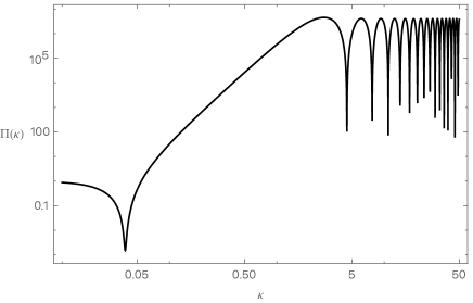
Figure 1: The quantity $\Pi(\kappa)$ introduced in eq (2.8), evaluated for $\Pi_{0}=10^{3}$.

Starting from eq (LABEL:solzm), we review for the rest of this section some of the results of [22] on the power spectrum of the curvature perturbation, evaluated at the end of inflation $\tau=0$. In the next section, then, we analyse the bispectrum. The power spectrum at the end of inflation is defined in terms of two point correlators of curvature perturbation

$$\langle\zeta_{\kappa}(\tau=0)\zeta_{\rho}(\tau=0)\rangle\,=\,\delta(\vec{\kappa}+\vec{\rho})\,P_{\kappa}\,.$$ (2.6)

At very large scales, $\kappa\ll 1$, the power spectrum acquires the usual scale invariant limit

$$P_{\kappa\ll 1}(\tau)\,=\,\frac{{\cal P}_{0}}{\kappa^{3}}\,,\hskip 14.22636pt{\rm with}\hskip 14.22636pt{\cal P}_{0}\,=\,\frac{H_{0}^{2}\,(-\tau_{1})^{3}}{4\epsilon_{1}}\,.$$ (2.7)

However, at smaller scales, the structure of the mode function (LABEL:solzm) leads to a rich scale dependence for the two point function. We define the dimensionless spectrum evaluated at the end of inflation:

$$\Pi(\kappa)\,=\,\frac{P_{\kappa}(\tau=0)}{P_{\kappa\ll 1}(\tau=0)}\,,$$ (2.8)

as a ratio between values of the spectrum at scale $\kappa$, versus the the spectrum at $\kappa=0$. Eq (LABEL:solzm) leads to

$${\Pi}(\kappa)\,=\,1+4\Pi_{0}\,\kappa\,j_{1}(\kappa)\left(\kappa j_{1}(\kappa)-j_{0}(\kappa)\right)+4\,\Pi_{0}^{4}\,\kappa^{2}j_{0}^{2}(\kappa)\,,$$ (2.9)

where

$$j_{0}(\kappa) = \frac{\sin\kappa}{\kappa}\hskip 19.91684pt;\hskip 19.91684ptj_{1}(\kappa)\,=\,\frac{\sin\kappa}{\kappa^{2}}-\frac{\cos\kappa}{\kappa}$$ (2.10)

are the spherical Bessel functions. The profile for the function ${\Pi}(\kappa)$ is represented in Fig 1. As anticipated, in the limit of infinitely large $|\eta|$, the $1/|\eta|$ corrections vanish and the resulting spectrum depends only on one parameter, $\Pi_{0}$. Corrections of order $1/|\eta|$ and higher can be computed starting with formulas of Appendix A. They improve the small scale behaviour reducing the amplitude of oscillations for $\kappa>1$ in Fig 1, but they do not affect the large scale profile $\kappa\leq 1$. It is clear that the amplitude of the spectrum increases considerably from large towards small scales, reaching its maximal values starting around $\kappa\sim{\cal O}(1)$. In fact, the parameter $\Pi_{0}$ in eq (2.3) has a transparent physical interpretation, since it controls the amplification of the spectrum between large and small scales (see [22] and Appendix A):

$$\frac{\lim_{\kappa\to\infty}P_{\kappa}(\tau=0)}{\lim_{\kappa\to 0}P_{\kappa}(\tau=0)}\,=\,\left(1+\Pi_{0}\right)^{2}\,.$$ (2.11)

If we wish a large value of $\Pi(\kappa)$ at small scales, as required in models leading to primordial black hole formation, then the value of the parameter $\Pi_{0}$ should be large. We assume this condition in what follows.

What is causing the rich scale dependence of the curvature spectrum, as represented in Fig 1? The responsible is the would-be decaying mode, that does not actually decay at superhorizon scales during the phase of non slowroll evolution. It is the disruptive interference between decaying and non decaying mode that produces the dip in the spectrum at intermediate scales, which is clearly visible in Fig 1. Moreover, also the rapid growth in the spectrum from large towards small scales (scaling with a slope $\kappa^{4}$ [98]) is caused by the decaying mode dynamics. See e.g. [11] for a review.

With the aid of our analytical formulas, it is not difficult to analytically determine the position of the dip in scenarios with large $\Pi_{0}$. We assume that the position of the dip is parametrised as $\kappa\,=\,x\,\sqrt{3/(2\Pi_{0})}$, with $x$ some dimensionless constant to be determined. We plug this Ansatz in (2.9), and expand the result for large $\Pi_{0}$. We find the expression

$$\Pi(x)\,=\,\left(1-x\right)^{2}+\frac{3x^{4}(6-x^{2})}{10\,\Pi_{0}}+{\cal O}\left(\frac{1}{\Pi_{0}^{2}}\right)\,.$$ (2.12)

The position of the dip in the spectrum corresponds to a choice of $x$ which makes the first contribution in the previous formula vanishing, leaving us with the remaining small contributions suppressed by powers of the small quantity $(1/\Pi_{0})$. This leads to the choice $x=1$, hence

$$\kappa_{\rm dip}\,=\,\sqrt{\frac{3}{2\Pi_{0}}}\hskip 19.91684pt;\hskip 19.91684pt{\Pi}(\kappa_{\rm dip})\,=\,\frac{3}{2\Pi_{0}}+{\cal O}\left(\frac{1}{\Pi_{0}^{2}}\right)\,.$$ (2.13)

Comparing formulas (2.11) and (2.13), we learn that the position of the dip with respect to the peak is proportional to the inverse fourth power of the total gain in magnitude of the spectrum from large to small scales [18]. The single parameter $\Pi_{0}$ hence characterize the spectrum and all its features.

The overall properties of the curvature spectrum we determined with the large $|\eta|$ approach to inflation are in common with several inflationary models leading to primordial black hole production, based on violations of slowroll conditions. Various other analytical studies based on different approaches, see e.g. [13, 14, 16, 17, 18, 19, 20, 21]. Our formulas have the nice feature of depending on a single parameter $\Pi_{0}$, with a clear physical interpretation. Moreover, the large $|\eta|$ approach is sufficiently flexible to be straightforwardly applicable to the computation of three point functions for curvature fluctuations, leading to novel analytical results for the bispectrum. We explore this topic in what comes next.

3 Large $|\eta|$ limit and non-Gaussianities

In the previous section, we shown how the large $|\eta|$ approach of limit (2.3) leads to a simple analytical expression for the power spectrum in eq (2.9). It depends on a single dimensionless parameter $\Pi_{0}$, and it has clear physical properties matching what found in more sophisticated inflationary models of primordial black holes. In this section, we study the implication of eq (2.3) for the curvature three point function and the associated bispectrum. The topic was briefly discussed in [22]. Here we investigate it more systematically. We will be able to determine fully analytical formulas for the bispectrum, including its scale and shape dependence, depending again on the single free parameter $\Pi_{0}$ introduced in (2.3).

It is well known that non-Gaussianities in the statistics of fluctuations can play an important role in the formation of primordial black holes from inflation, for example since it affects the estimates of the threshold of PBH formation. See e.g. [31, 32, 33, 34, 36, 37, 38, 39, 40, 41, 42, 43, 44, 45, 48, 49, 50, 51, 52, 53, 54] for works studying different aspects of this topic. In many studies, it is customary to consider primordial non-Gaussianity with a local form. In this work we analytically compute the bispectrum from first principles using the in-in formalism, in the large $|\eta|$ limit of inflation. We show that non-Gaussian features are characterised by a rich shape and scale dependence.

Our assumptions for the behaviour of the system – quasi de Sitter slowroll expansion throughout the inflationary era, a part from a brief phase of large $|\eta|$ evolution – help us to uniquely characterise the structure of the curvature three point function. The third order interaction Hamiltonian for curvature perturbations in single field inflation [99] contains one term which gives the dominant contribution to the bispectrum [75, 76]

$${\cal H}_{\rm int}(\tau)\,=\,-\frac{1}{2}\,\int d^{3}x\,a^{2}(\tau)\,\epsilon(\tau)\,\eta^{\prime}(\tau)\,\zeta^{2}(\tau,\vec{x})\,\zeta^{\prime}(\tau,\vec{x})\,.$$ (3.1)

Since this contribution depends on the time derivative $\eta^{\prime}(\tau)$, it is proportional to the large jump in the $\eta$ parameter occurring at the beginning ($\tau=\tau_{1}$) and at the end ($\tau=\tau_{2}$) of the non slowroll phase. Being this epoch extremely brief in our framework, we have no option but to consider a sudden transition among different evolution eras. We can then express the time derivative of the $\eta$ parameter, as appearing in eq (3.1), as [76]

$$\eta^{\prime}(\tau) = \Delta\eta\left[-\delta(\tau-\tau_{1})+\delta(\tau-\tau_{2})\right]\,,$$ (3.2)

the quantity $\Delta\eta$ in eq (3.2) controls the jump of the $\eta$ parameter. We will soon determine its precise value, making use of appropriate physical arguments.

But first, we use the interaction Hamiltonian (3.1) to write a formal expression for the bispectrum $B_{\zeta}$ at the end of inflation, $\tau=0$, defined by means of the formula:

$$\langle\zeta_{\kappa_{1}}(0)\zeta_{\kappa_{2}}(0)\zeta_{\kappa_{3}}(0)\rangle\,=\,\delta({\vec{\kappa}}_{1}+{\vec{\kappa}}_{2}+{\vec{\kappa}}_{3})\,B_{\zeta}(\kappa_{1},\kappa_{2},\kappa_{3})\,.$$ (3.3)

As usual, momentum conservation requires that the vectors labelling the perturbations in Fourier space form a closed triangle. The in-in formalism prescribes to compute the three-point correlator as

$$\langle{\rm in}\Big{|}{\bar{T}}e^{-i\int{\cal H}_{\rm int}(\tau^{\prime})d\tau^{\prime}}\,\zeta_{\kappa_{1}}(0)\zeta_{\kappa_{2}}(0)\zeta_{\kappa_{3}}(0)\,{T}e^{i\int{\cal H}_{\rm int}(\tau^{\prime})d\tau^{\prime}}\Big{|}{\rm in}\rangle\,.$$ (3.4)

Using the Ansatz (3.2), we obtain the following structure [76]

$$B_{\zeta}(\kappa_{1},\kappa_{2},\kappa_{3})=$$

$$-2\Delta\eta\Big{(}\epsilon(\tau_{2})a^{2}(\tau_{2})\,{\rm Im}\left[\left(\zeta_{\kappa_{1}}(0)\zeta^{*}_{\kappa_{1}}(\tau_{2})\right)\left(\zeta_{\kappa_{2}}(0)\zeta^{*}_{\kappa_{2}}(\tau_{2})\right)\left(\zeta_{\kappa_{3}}(0)\partial_{\tau_{2}}\zeta^{*}_{\kappa_{3}}(\tau_{2})\right)\right]-(\tau_{2}\to\tau_{1})\Big{)}$$

$$+{\rm perms\,.}$$ (3.5)

To proceed with the computations, we now determine the value of $\Delta\eta$ in eq (3.5).

The value of $\Delta\eta$, and the resulting structure of the bispectrum

We start computing the squeezed limit of the expression (3.5). Formally it reads

$$\lim_{q\to 0}B_{\zeta}(\kappa,\kappa,q)$$

$$=\,-\,4\Delta\eta\,\epsilon(\tau_{2})a^{2}(\tau_{2})\,|\zeta_{q}(0)|^{2}\,|\zeta_{\kappa}(0)|^{2}$$

$$\times\left\{{\rm Im}\left[\frac{\zeta_{\kappa}^{2}(0)}{|\zeta_{\kappa}(0)|^{2}}\zeta_{\kappa}^{*}(\tau_{2})(\zeta^{\prime}_{\kappa}(\tau_{2}))^{*}\right]-\frac{\epsilon(\tau_{1})a^{2}(\tau_{1})}{\epsilon(\tau_{2})a^{2}(\tau_{2})}{\rm Im}\left[\frac{\zeta_{\kappa}^{2}(0)}{|\zeta_{\kappa}(0)|^{2}}\zeta_{\kappa}^{*}(\tau_{1})(\zeta^{\prime}_{\kappa}(\tau_{1}))^{*}\right]\right\}\,.$$

(3.6)

In absence of a phase of slowroll violation, the squeezed limit of the previous formula satisfies Maldacena consistency relation [99]:

$$\lim_{q\to 0}B(\kappa,\kappa,q) = -\left(n_{\zeta}(\kappa)-1\right)\,|\zeta_{q}(0)|^{2}\,|\zeta_{\kappa}(0)|^{2}\,,$$ (3.7)

with $(n_{\zeta}(\kappa)-1)=d\ln\Pi(\kappa)/d\ln\kappa$. In our case, we can expect the consistency relation (3.7) to be satisfied for small $\kappa$, in a regime $q\ll\kappa\ll 1$. In fact, modes with such small values of momenta leave the horizon early in the inflationary phase, well before the non slowroll epoch occurs. Correspondingly, the decaying mode has long time to decay: it can not be significantly resurrected by the non slowroll phase, which occurs much later than its horizon crossing. We can then plug the mode functions determined in Appendix A into eq (3.6). We expand for small $\kappa$, and we impose the validity of (3.7) up to order $\kappa^{2}$. This procedure determines uniquely the parameter $\Delta\eta$ in the large $|\eta|$ limit of eq (2.3). We find

$$\Delta\eta\,=\,\frac{|\eta|}{(1+\Pi_{0})}+\frac{\Pi_{0}(12+34\Pi_{0}+25\Pi_{0}^{2})}{2(1+\Pi_{0})^{2}(1+2\Pi_{0})}\,,$$ (3.8)

up to corrections of order $1/|\eta|$.

Armed with the precise value of $\Delta\eta$, as well as with the mode functions computed in Appendix A, we can analytically evaluate the full bispectrum using eq (3.5). The overall coefficient (proportional to $\Delta\eta$) scales as $|\eta|$. But taking differences over mode functions within the parenthesis of (3.5), we find that they scale as $1/|\eta|$, compensating for the overall large factor $|\eta|$. Taking the limit (2.3) of large $|\eta|$ we obtain a finite, well defined result for the bispectrum. Its structure is

$$B_{\zeta}\left(\kappa_{1},\kappa_{2},\kappa_{3}\right)\,=\,{\cal P}_{0}^{2}\,{\cal A}_{\zeta}\left(\kappa_{1},\kappa_{2},\kappa_{3}\right)\,,$$ (3.9)

with ${\cal P}_{0}$ given in eq (2.7), while the dimensionless function ${\cal A}$ is built in terms of the combination

$${\cal A}_{\zeta}\left(\kappa_{1},\kappa_{2},\kappa_{3}\right)\,=\,\sum_{n=1,\dots,4}\,{\cal C}_{n}\left(\kappa_{1},\kappa_{2},\kappa_{3}\right)\,\Pi_{0}^{n}\,.$$ (3.10)

The analytical expression for the functions ${\cal C}_{n}$ can be found in Appendix B. They are oscillatory functions of combinations of momenta. The resulting bispectrum has a rich momentum and shape dependence, which we explore in what follows.

The squeezed (and not-so-squeezed) limit of the bispectrum

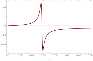
Figure 2: Left: the squeezed bispectrum satisfies Maldacena consistency relation. Red: $(1-n_{\zeta})$, Dashed black the squeezed non-linear parameter $5\,f_{\rm NL}^{\rm sq}/6$ defined in eq (3.11). Right: The function $G(\kappa)$ defined in eq (3.13), divided by $\Pi_{0}^{2}$ (black line). The quantity $(ns-1)/2$ divided by $\Pi_{0}^{1/2}$ (dashed blue line). The normalization factors are introduced to obtain comparable variables for the two quantities introduced. In both panels, $\Pi_{0}=10^{3}$.

The squeezed limit of the bispectrum (3.9) can be studied analytically. It satisfies Maldacena consistency relation for any value of $\kappa$. Defining

$$\lim_{q\to 0}{\cal A}\left(\kappa,\kappa,q\right)\,=\,\frac{6}{5}\,f_{\rm NL}^{\rm sq}\,\frac{\Pi(\kappa)}{\kappa^{3}}\frac{\Pi(q)}{q^{3}}\,,$$ (3.11)

we have the relation

$$f_{\rm NL}^{\rm sq}(\kappa)\,=\,\frac{5}{6}\,\left(1-n_{\zeta}(\kappa)\right)\,.$$ (3.12)

See Fig 2, left panel. This result might appear surprising, since it is well known that Maldacena consistency relation can be violated in scenarios which include ultra slowroll phases (see e.g. [100, 92, 101]). Our result of eq (3.12) indicates the duration (2.2) of the non slowroll era is too brief for triggering a violation of the consistency condition – no matter how large $|\eta|$ is.

As manifest in Fig 2, left panel, the squeezed limit of the bispectrum is strongly scale dependent, reaching its extrema in the region $\kappa_{\rm dip}$ around the dip in the spectrum, to then assume values of order one (and negative) for scale $\kappa\sim{\cal O}(1)$ towards the first peak of the spectrum. (See e.g. [102, 103, 104] for early works on scale dependent non-Gaussianities.) Again, the features of $f_{\rm NL}^{\rm sq}$ are determined by the single parameter $\Pi_{0}$ controlling the spectrum.

Since we have analytical control of the bispectrum, we can also investigate the first order corrections ${\cal O}(q^{2})$ to the squeezed bispectrum. Such contributions can be associated with the curvature of the background, see e.g. [105]. They can manifest significant deviations from the predictions of standard slowroll scenarios. We parameterise such corrections in terms of a function $G(\kappa)$:

$$\lim_{q\ll 1}{\cal A}\left(\kappa,\sqrt{\kappa^{2}+q^{2}},q\right)\,=\,-\left(n_{\zeta}(\kappa)-1\right)\,\frac{\Pi(\kappa)}{\kappa^{3}}\frac{\Pi(q)}{q^{3}}+q^{2}\,\frac{\Pi(\kappa)}{\kappa^{3}}\frac{\Pi(q)}{q^{3}}\,G(\kappa)+{\cal O}(q^{3})\,.$$ (3.13)

In computing the next-to-leading corrections (3.13), we focus on momenta forming a right triangle, with one of the catheti corresponding to the small momentum $q$. We represent in Fig 2, right panel, the function $G(\kappa)$ controlling the correction $q^{2}$ in eq (3.13) (normalized by inverse powers of $\Pi_{0}$). As apparent from the figure, this function has a distinctive feature around the position $\kappa_{\rm dip}$ of the dip of the spectrum. This feature can be interpreted as due to the decaying mode, that influences the dynamics around $\kappa_{\rm dip}$. The amplitude of this feature is parametrically larger by a factor of order $\Pi_{0}^{3/2}$ with respect to the feature associated with the spectral index and $f_{\rm NL}^{\rm sq}$ (which we represent for comparison in Fig 2). This indicates that the effects of the would-be decaying mode and of the non slowroll phase – controlled by $\Pi_{0}$ – become more and more accentuated as we leave the squeezed limit. In fact, we will now find further manifestations of the would-be decaying mode dynamics by studying other shapes of the bispectrum.

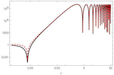
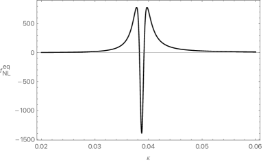
Figure 3: Left: The right hand side of eq (3.14) (black line) versus the left hand side of the same equation (dashed red line) Right: The quantity $f_{\rm NL}^{\rm eq}$ defined in eq (3.15). In both panels, $\Pi_{0}=10^{3}$.

.

The equilateral shape of the bispectrum

For an equilateral bispectrum, where all momenta have the same size $\kappa$, we find interesting overlaps between the scale dependent profiles of the bispectrum and of the power spectrum. Recall the expressions for the dimensionless quantities ${\cal A}$ and ${\Pi}$ in eqs (3.10) and (2.9). We find the relation

$$\frac{\kappa^{4}}{6\Pi_{0}}\,\big{|}{\cal A}_{\zeta}(\kappa,\kappa,\kappa)\big{|}\,\simeq\,\Pi^{3/2}(\kappa)\,,$$ (3.14)

is very well satisfied for the entire range of scales, see Fig 3, left panel. Again, we interpret this behaviour as due to the dynamics of the decaying mode, that increases the magnitude of the equilateral bispectrum in a similar way as it does for the power spectrum.

As customary, we define the dimensionless parameter $f_{\rm NL}^{\rm eq}$

$$f_{\rm NL}^{\rm eq}(\kappa)\,=\,\frac{5}{18}\,\frac{B_{\zeta}(\kappa,\kappa,\kappa)}{P_{\kappa}^{2}}\,=\,\frac{5}{18}\,\frac{\kappa^{6}\,{\cal A}_{\zeta}(\kappa,\kappa,\kappa)}{\Pi^{2}(\kappa)}\,,$$ (3.15)

controlling the size of the equilateral bispectrum with respect to the power spectrum, and represent its scale-dependent profile in Fig 3, right panel. The size of $f_{\rm NL}^{\rm eq}$ is relatively small at all scales, a part from the region around $\kappa_{\rm dip}=\sqrt{3/(2\Pi_{0})}$, where it develops pronounced features. (See also [106, 107] for related computations using a different approach based on [15].)

A very similar behaviour occurs for other non-Gaussian shapes as well, and can be studied with our analytic formula (3.10). To conclude this section, we investigate the shape dependence of the bispectrum using a convenient graphical representation in terms of triangular plots.

Graphical representation of more general shapes of the bispectrum

For representing the shape dependence of the bispectrum as a function of the scale, we use the graphical device introduced in [108] (see also [12] for a pedagogical review). We define the function

$$S(\kappa_{1},\kappa_{2},\kappa_{3})\,=\,N\,\kappa_{1}^{2}\,\kappa_{2}^{2}\,\kappa_{3}^{2}\,B_{\zeta}(\kappa_{1},\kappa_{2},\kappa_{3})\,,$$ (3.16)

where the normalization constant $N$ is selected such that $S(1,1,1)\,=\,1$. We then introduce the coordinates $x_{2}\,=\,\kappa_{2}/\kappa_{1}$, $x_{3}\,=\,\kappa_{3}/\kappa_{1}$, and represent the magnitude of $S(\kappa,x_{2},x_{3})$ in triangular plots as in Fig 4. Ordering momenta such that $x_{3}\leq x_{2}\leq 1$, the triangular inequality requires $x_{2}+x_{3}>1$. To avoid representing configurations which are equivalent, we only focus on the region $1-x_{2}\leq x_{3}\leq x_{2}$. Given the fact that our bispectrum is strongly dependent on the scale, the result depends on the choice of the first argument $\kappa$ in the quantity $S(\kappa,x_{2},x_{3})$. We make the two choices $\kappa=\kappa_{\rm dip}$ and $\kappa=1$. While for $\kappa=1$ the bispectrum is mostly enhanced for the equilateral shape, the behaviour at $\kappa_{\rm dip}$ is more rich, and the spectrum is enhanced for elongated triangles, where the size of two of the momenta is well larger than the third one. Hence, depending on the scales one considered, different shapes can become dominant, with distinct consequences for observables controlling the physics of PBH.

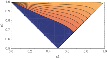
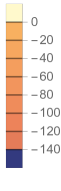
Figure 4: Triangular plots of the function $S(\kappa,x_{2},x_{3})$ of eq (3.16), represented with the criteria discussed in the text. Left $S(\kappa_{\rm dip},x_{2},x_{3})$. Right $S(1,x_{2},x_{3})$.

In fact, is there any specific physical implication for the rich scale dependence of the bispectrum in our system, as we explored so far? In the next section, we will study some consequences of our findings for the statistics of scalar-induced gravitational waves.

4 Gravitational waves and non-Gaussianity

In the investigations we carried on so far, we demonstrated that the analytical bispectrum of eq (3.10) has a rich shape and scale dependence, more complex than a pure local-type non-Gaussian statistics. The information we obtained can be important when studying observables that involve convolution integrals over all scales. Such quantities can in fact be sensitive to the large scale features of the bispectrum we investigated in section 3.

Explicit examples are observables built in terms of tensor modes sourced at second order by scalar fluctuations which are enhanced at small scales, for example by non slowroll epochs as we considered in sections 2 and 3. See e.g. [56, 57, 58, 59, 60, 61, 62, 63] for some of the original papers on the subject, and [64] (and references therein) for a comprehensive review. Integrations involving convolutions depend on the power spectrum and bispectrum at all scales. Hence they can be sensitive to the features of the statistics of fluctuations that we studied in the previous section. We proceed to study this phenomenon explicitly.

Schematically, scalar perturbations with an enhanced curvature spectrum $P_{\zeta}(k)$ (recall its definition in eq (2.6)) can source a tensor spectrum $P_{h}$ at second order in fluctuations

$$P_{h}(k)\,=\,\int dk^{\prime}\,f(k,k^{\prime})\,P_{\zeta}(k^{\prime})\,P_{\zeta}(k-k^{\prime})\,,$$ (4.1)

where $f(k,k^{\prime})$ is a kernel function depending on cosmology. For convenience, in this section we make use of dimensionful momenta $k$: their dimensionless version $\kappa$ can be easily obtained in terms of the definition (2.4). Expressions as (4.1) are derived under the hypothesis of Gaussian primordial curvature fluctuations. Local type non-Gaussianity can modulate the scale dependence of the induced tensor spectrum, with interesting phenomenological implications [65, 66, 67, 68, 69, 70, 71, 72]. Here we explore the implications of an enhanced curvature bispectrum for another interesting observable: the tensor-tensor-scalar bispectrum $B_{TTS}$ evaluated during radiation domination. The quantity $B_{TTS}$ involves two (scalar induced) tensor modes $h$ and one Bardeen scalar mode $\Phi$. Schematically, in the squeezed limit we expect a relation like the following one (soon we will be more precise)

$$B_{TTS}(k_{1},k_{2},k_{3})\,=\,\int dq\,\tilde{f}(k_{1},k_{2},q)\,B_{\zeta}(k_{1},k_{2},q)\,P_{\zeta}(k_{1}-q)\,,$$ (4.2)

for $\tilde{f}$ some kernel function. A squeezed version of the bispectrum of eq (4.2) can correlate (scalar induced) stochastic backgrounds probed by gravitational wave experiments at small scales, with a large scale scalar modes probed by cosmic microwave background observations. It is the observable investigated in [73] (see also [109, 110, 111, 112, 113, 114, 115, 116, 117]) for carrying on a ‘multimessenger cosmology’ program. It suggests new experimental avenues for probing the physics of early universe, and its detection and characterization would provide a smoking gun for the primordial origin of the gravitational stochastic background. Besides the squeezed limit, the bispectrum $B_{TTS}$ might be phenomenologically relevant for other elongated shapes also, above all if its size is large

We leave these interesting phenomenological applications aside, and we proceed with computing more precisely the observable $B_{TTS}$ described above eq (4.2). The actual computations are rather technical, and we relegate them to Appendix C. Let us start discussing the results for the squeezed limit, where expressions simplify. We find ($k_{1}=k_{2}=k$)

$$\lim_{k_{3}\to 0}B_{TTS}(k,k,k_{3})\,=\,\frac{12}{5}\,f_{\rm NL}^{TTS}(k)\,P_{h}(k)P_{\zeta}(k_{3})\,,$$ (4.3)

where

$$f_{\rm NL}^{TTS}(\tau,k)\equiv\frac{5}{12}\,\frac{\int d^{3}q\,{{P}_{\zeta}(|\vec{k}-\vec{q}|)}{{P}_{\zeta}(q)}\,\,\left[1-n_{\zeta}(q)\right]\,{\cal F}_{0}(\tau,\vec{k},\vec{q})}{\int d^{3}q\,{{P}_{\zeta}(|\vec{k}-\vec{q}|)}{{P}_{\zeta}(q)}\,{\cal F}_{0}(\tau,\vec{k},\vec{q})}\,,$$ (4.4)

while the tensor spectrum is

$$P_{h}(\tau,k)\,=\,\int d^{3}q\,{{P}_{\zeta}(|\vec{k}-\vec{q}|)}{{P}_{\zeta}(q)}\,{\cal F}_{0}(\tau,\vec{k},\vec{q})\,.$$ (4.5)

The explicit expression for the kernel function ${\cal F}_{0}$ can be found in eq (C.12). In writing eq (4.4) we use the fact that the squeezed limit of the scalar bispectrum satisfies Maldacena consistency relation, see section 3.

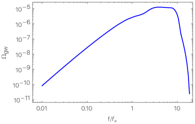
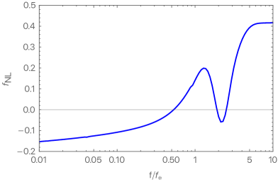
Figure 5: Left: plot of the gravitational wave energy density induced by a scalar spectrum derived from eq (4.5), with $\Pi_{0}=10^{3}$, under the conditions discussed in the main text. Right: plot of the non-linear parameter $f_{\rm NL}^{TTS}$ in eq (4.4) computed with the same curvature spectrum of the left figure.

Starting from eq (4.5) it is straightforward to derive the expression for the gravitational wave energy density $\Omega_{\rm GW}$, and perform the integrals numerically by implementing the convenient formulas of [118]. We represent the result in Fig 5, left panel, where we compute the $\Omega_{\rm GW}$ induced by the analytical scalar spectrum of eq (3.9). To avoid numerical issues, we smoothed out the oscillatory features occurring at small scales $\kappa>1$, and we truncated the power at $\kappa=10$ (i.e. we set $\Pi(\kappa)=0$ for $\kappa>10$). We converted to frequency $f=2\pi k$. The result is a broad gravitational spectrum, with an ample plateau for $1\leq f/f_{*}\leq 10$, with $f_{*}$ a reference frequency. See Fig 5, left panel. In Fig 5, right panel, we represent the non linear parameter $f_{\rm NL}^{TTS}$ introduced in eq (4.4), computed starting from the curvature power spectrum as described above. $f_{\rm NL}^{TTS}$ has a strong dependence on the scale, and its typical magnitude is not large, being of the order of $10^{-1}$. It has an oscillatory behaviour of $f_{\rm NL}^{TTS}$ at frequencies around the peak of the tensor spectrum. We interpret it as a consequence of the sign change and amplified features of the scalar spectral index $n_{\zeta}(\kappa)-1$ appearing in the integrand of eq (4.4) (see Fig 2), which are amplified where the tensor spectrum is most enhanced. It would be interesting to explore whether other shapes can reach larger magnitudes in this set-up.

In fact, the general structure of the $B_{TTS}$ bispectrum is given in eq (C.16), which we report here:

$$B_{TTS}(\vec{k}_{1},\vec{k}_{2},\vec{k}_{3}) = \int d^{3}q\,{{P}_{\zeta}(|\vec{k}_{1}-\vec{q}|)}\,B_{\zeta}\left(q,|\vec{k}_{3}+\vec{q}|,k_{3}\right)\,{\cal F}_{1}(\tau,\vec{k}_{1},\vec{k}_{3},\vec{q})$$ (4.6)

$$+ {{P}_{\zeta}(k_{3})}\int d^{3}q\,\,B_{\zeta}\left(|\vec{k}_{1}+\vec{k}_{3}|,|\vec{q}+\vec{k}_{1}+\vec{k}_{3}|,q\right)\,{\cal F}_{2}(\tau,\vec{k}_{1},\vec{k}_{3},\vec{q})\,,$$

where the quantities ${\cal F}_{1,2}$ can be found in eqs (C.17) and (LABEL:defbf2). Such expression shows that the scale and shape dependence of the bispectrum can play an important role. For example, going beyond the squeezed limit (considering the leading $k_{3}^{2}$ corrections to eq (4.3), which might still be relevant for coupling large and small scale modes) the convolution integral in the second line in eq (4.6) starts to contribute to the result, in a way that depends on shapes of the bispectrum different from the local one. We learned in section 3 how the effects of the non slowroll phase, and of a large parameter $\Pi_{0}$, can considerably influence the amplitude of the bispectrum for shapes different from local. It will be important to further study the behaviour of $B_{TTS}$ for general shapes and its phenomenological consequences.

While in this work we focussed on the bispectrum, the large $|\eta|$ approach can also be applied to compute the trispectrum at leading order in $1/|\eta|$. We are hopeful that, starting from the fourth order interaction Hamiltonian, and proceeding as in section 3, a full analytic expression for the scalar trispectrum can be determined. We expect such expression to exhibit a rich shape and scale dependence, as we found for the bispectrum. Such result would be relevant for the computation of the induced spectrum of gravitational waves, that through convolution integrals is modulated by the trispectrum [69, 71, 74]. While most of works so far focussed on local type non-Gaussian correlators, it would be interesting to extend computations to the case of a more complex trispectrum derived from first principle calculations in the $1/|\eta|$ limit.

Acknowledgments

It is a pleasure to thank Jacopo Fumagalli for discussions and Ameek Malhotra for feedback. GT is partially funded by the STFC grants ST/T000813/1 and ST/X000648/1. For the purpose of open access, the author has applied a Creative Commons Attribution licence to any Author Accepted Manuscript version arising.

Appendix A The mode functions during the brief non slowroll phase

In this Appendix we briefly review the results of [18] which analytically compute the solution for mode functions in a scenario of inflation undergoing a brief, but drastic phase of non slowroll evolution. We parameterize the background evolution as constituted by three phases:

1. An initial slowroll phase, where the slowroll parameters $\epsilon$ and $\eta$ are very small and the evolution can be approximated as de Sitter phase. The constant value of the parameter $\epsilon$ is denoted with $\epsilon_{1}$.

2. A second, brief non slowroll epoch lasting between two conformal times $\tau_{1}$ and $\tau_{2}$. The parameter $\eta$ is negative and large in absolute magnitude, while the small, time dependent parameter $\epsilon(\tau)$ rapidly decreases (and the Hubble parameter remains almost constant).

3. Finally a third era of slowroll evolution for $\tau_{2}\leq\tau\leq 0$, where $\epsilon$ and $\eta$ are both small and constant. The value of the parameter $\epsilon$ in this phase is denoted with $\epsilon_{2}$.

We rescale the curvature perturbation $\zeta_{k}(\tau)$ as

$$\varphi_{k}(\tau)\,=\,z(\tau)\,{\zeta_{k}(\tau)}\,.$$ (A.1)

The Mukhanov-Sasaki equation for the variable $\varphi_{k}(\tau)$ reads

$$\varphi_{k}^{\prime\prime}(\tau)+\left(k^{2}-\frac{z^{\prime\prime}(\tau)}{z(\tau)}\right)\,\varphi_{k}(\tau)=\,0\,.$$ (A.2)

The general expression of the pump field $z(\tau)$ is

$$z(\tau)\,=\,a(\tau)\sqrt{2\epsilon(\tau)}\,.$$ (A.3)

Given the conditions described above, in a quasi de Sitter limit the pump field can be paramaterised as follows

$$z(\tau)\,=\,\begin{cases}-\frac{\sqrt{2\,\epsilon_{1}}}{H_{0}\,\tau}&{\text{for $\tau\leq\tau_{1}$}}\\ \\ -\frac{\sqrt{2\,\epsilon(\tau)}}{H_{0}\,\tau}&{\text{for $\tau_{1}\leq\tau\leq\tau_{2}$}}\\ \\ -\frac{\sqrt{2\,\epsilon_{2}}}{H_{0}\,\tau}&{\text{for $\tau_{2}\leq\tau\leq 0$}}\end{cases}$$ (A.4)

with $\epsilon(\tau)$ a continuous function, and $H_{0}$ the (nearly constant) Hubble parameter during inflation. We define the parameter $\eta$ as

$$\eta\,=\,-\lim_{\tau\to\tau_{1}^{+}}\,\frac{d\ln\epsilon(\tau)}{d\ln\tau}\,,$$ (A.5)

and we consider it constant, negative, and large in absolute value.

We parameterize the solution of Mukhanov-Sasaki equation (A.2) in terms of the following formal series

$$\varphi_{k}(\tau)\,=\,-i\frac{H_{0}\,e^{-ik\tau}}{2\sqrt{\epsilon_{1}\,k^{3}}}\,z(\tau)\,\left[1+ik\tau+(ik\tau_{1})^{2}A_{(2)}(\tau)+(ik\tau_{1})^{3}A_{(3)}(\tau)+\dots\right]\,,$$ (A.6)

where the functions $A_{(n)}(\tau)$, $n\geq 2$, have to be determined. Plugging the Ansatz (A.6) into the Mukhanov Sasaki eq (A.2), we find the following coupled system of equations for the quantities $A_{n}(\tau)$:

$$\left[\frac{\epsilon(\tau)}{\tau^{2}}\,\tau_{1}^{2}\,A_{(2)}^{\prime}(\tau)\right]^{\prime} = \frac{\epsilon^{\prime}(\tau)}{\tau}\,,$$ (A.7)

$$\left[\frac{\epsilon(\tau)}{\tau^{2}}\,\left(\tau_{1}\,A_{(n)}^{\prime}(\tau)-A_{(n-1)}(\tau)\right)\right]^{\prime} = \frac{\epsilon(\tau)\,A_{(n-1)}^{\prime}(\tau)}{\tau^{2}}\hskip 19.91684pt,{\text{for $n>2$}}\,.$$ (A.8)

If $\epsilon(\tau)$ is constant, then a consistent solution is $A_{(n)}=0$ for $n\geq 2$, and eq (A.6) reduces to the usual solution for mode functions in the de Sitter limit. But we are interested on evaluating the effects a time dependent $\epsilon(\tau)$ (and a large $\eta$ parameter) during the non slowroll phase of evolution. A formal solution for eq (A.7) is

$$\tau_{1}^{2}\,A_{(2)}(\tau)\,=\,\int_{-\infty}^{\tau}\,d\tau_{a}\,\frac{\tau_{a}^{2}}{\epsilon(\tau_{a})}\,\left(\int_{-\infty}^{\tau_{a}}\,d\tau_{b}\,\frac{\epsilon^{\prime}(\tau_{b})}{\tau_{b}}\right)\,.$$ (A.9)

For $\tau<\tau_{1}$, the $\epsilon$ parameter is constant and $A_{(2)}(\tau)$ vanishes as desired: it acquires a non-zero value starting from $\tau=\tau_{1}$ onwards.

Considering values of $A_{(n)}(\tau)$ for $n>2$, we find the following formal solution for eq (A.8):

$$\tau_{1}\,A_{(n)}(\tau)\,=\,\int_{-\infty}^{\tau}d\tau_{a}\,A_{(n-1)}(\tau_{a})+\int_{-\infty}^{\tau}\,d\tau_{a}\,\frac{\tau_{a}^{2}}{\epsilon(\tau_{a})}\left(\int_{-\infty}^{\tau_{a}}\,d\tau_{b}\,\frac{\epsilon(\tau_{b})\,A_{(n-1)}^{\prime}(\tau_{b})}{\tau_{b}^{2}}\right)\,.$$ (A.10)

Interestingly, we can now exploit the fact that the duration of the non slowroll phase is small, $-(\tau_{2}-\tau_{1})/\tau_{1}\ll 1$. We expand in Taylor series the previous formal solutions, focussing on the leading term (more details in [18]). For $A_{(2)}$ we find, when evaluated at $\tau_{1}\leq\tau\leq\tau_{2}$:

$$A_{(2)}(\tau) = \left(\frac{d\ln\epsilon(\tau)}{d\ln\tau}\right)_{\tau=\tau_{1}}\,\frac{\left(\tau-\tau_{1}\right)^{2}}{\tau_{1}^{2}}+{\cal O}\left[(\tau-\tau_{1})^{3}\right]\,,$$ (A.11)

$$= -\eta\,\frac{1}{2}\,\frac{\left(\tau-\tau_{1}\right)^{2}}{\tau_{1}^{2}}+{\cal O}\left[(\tau-\tau_{1})^{3}\right]\,.$$

Proceeding analogously and Taylor expanding for higher $n$, we find the following leading contributions

$$A_{(n)}(\tau) = -\eta\,\frac{2^{n-2}}{n!}\,\frac{\left(\tau-\tau_{1}\right)^{n}}{\tau_{1}^{n}}\,,\hskip 19.91684pt{\text{for $n\geq 2$}}\,.$$ (A.12)

Plugging the solutions of eq (A.12) into eq (A.6), one finds an exponential series, which can be resummed giving

$$\varphi_{k}(\tau)\,=\,-i\frac{H_{0}\,e^{-ik\tau}}{2\sqrt{\epsilon_{1}\,k^{3}}}\,z(\tau)\,\left[1+ik\tau+\frac{\eta}{4}\left(1+2ik\left(\tau-\tau_{1}\right)-e^{2ik(\tau-\tau_{1})}\right)\right]\,\hskip 14.22636pt{\text{for $\tau_{1}\leq\tau\leq\tau_{2}$}}\,.$$ (A.13)

This expression, valid for $\tau\leq\tau_{2}$, can then be matched to a solution of Mukhanov-Sasaki equation in the interval $\tau_{2}\leq\tau\leq 0$. Recall that in this epoch we return to a slowroll regime where $\epsilon$ and $\eta$ are negligibly small, hence the most general solution for the mode function is

$$\varphi_{k}(\tau)\,=\,-i\,{\cal K}_{1}\frac{H_{0}\,e^{-ik\tau}}{2\sqrt{\epsilon_{1}\,k^{3}}}\,z(\tau)\,\left(1+ik\tau\right)-i\,{\cal K}_{2}\frac{H_{0}\,e^{ik\tau}}{2\sqrt{\epsilon_{1}\,k^{3}}}\,z(\tau)\,\left(1-ik\tau\right)\,.$$ (A.14)

The scale dependent quantities ${\cal K}_{1,2}$ are determined by Israel matching the expression (A.14) with the solution (A.6) at time $\tau_{2}$. Defining $\Delta\tau=-(\tau_{2}-\tau_{1})/\tau_{1}$, the result is

$${\cal K}_{1} = 1-\frac{\eta}{8(1-\Delta\tau)^{2}\,k^{2}\,\tau_{1}^{2}}\left[1-e^{-2ik\tau_{1}\,\Delta\tau}+k\tau_{1}\,\Delta\tau\left(i+2k\tau_{1}(1-\Delta\tau)\right)\right]\,,$$ (A.15)

$${\cal K}_{2} = \frac{\eta e^{-2ik\tau_{1}\,(1-\Delta\tau)}}{8(1-\Delta\tau)^{2}\,k^{2}\,\tau_{1}^{2}}\left[1+2ik\tau_{1}-e^{-2ik\tau_{1}\,\Delta\tau}\left(i+2k\tau_{1}(1-\Delta\tau)\right)\right]\,.$$ (A.16)

It is straightforward to compute the two point function for curvature perturbations at the end of inflation $\tau=0$ in terms of $|\varphi_{k}(\tau)|^{2}$ using eqs (A.14) and (A.15), (A.16). The result can be used to prove eq (2.11) in the main text (see also [18]). Taking the large $|\eta|$ limit following eq (2.3), one recovers the expression (LABEL:solzm) in the main text (expressed in terms of the dimensionless momenta $\kappa$ defined in eq (2.4)).

Appendix B Explicit expressions for the coefficients ${\cal C}_{n}$

In this Appendix we collect the explicit functions ${\cal C}_{n}$, $n=1,\dots 4$, which form the analytic scalar bispectrum of eq (3.9). After defining

$$\Delta_{pq} = 1+\delta_{pq}\hskip 17.07182pt,\hskip 17.07182pt\Delta_{pqr}\,=\,\left(1+\delta_{pq}\right)\left(1+\delta_{qr}+\delta_{pr}\right)$$ (B.1)

we make use of the convenient combinations

$$K_{p} = \sum_{i}\,k_{i}^{p}\,,$$ (B.2)

$$K_{pq} = \frac{1}{\Delta_{pq}}\sum_{i\neq j}\,k_{i}^{p}k_{j}^{q}\,,$$ (B.3)

$$K_{pqr} = \frac{1}{\Delta_{pqr}}\sum_{i\neq j\neq\ell}\,k_{i}^{p}k_{j}^{q}k_{\ell}^{r}\,,$$ (B.4)

introduced in [119]. The previous combinations allow us to express the functions ${\cal C}_{n}$ as

$${\cal C}_{1} = \frac{\left(K_{114}+3K_{123}+6K_{222}-K_{4}-2K_{13}-2K_{22}-2K_{112}\right)}{K_{333}}\,j_{1}(\kappa_{1}+\kappa_{2}+\kappa_{3})$$ (B.5)

$$+\frac{\left(K_{14}+3K_{23}+2K_{113}+2K_{112}\right)}{K_{333}}\,j_{0}(\kappa_{1}+\kappa_{2}+\kappa_{3})$$

$${\cal C}_{2} = \frac{1}{K_{444}}\Big{[}10K_{134}+14K_{233}+9K_{224}+2K_{125}-K_{112}-K_{13}$$

$$-K_{24}-3K_{222}-K_{15}-2K_{123}-3K_{114}\Big{]}\,j_{0}(\kappa_{1}+\kappa_{2}+\kappa_{3})$$

$$+\frac{1}{K_{444}}\Big{[}K_{225}+7K_{234}+18K_{333}+3K_{113}+2K_{122}+K_{23}$$

$$-12K_{113}-3K_{115}-9K_{124}-13K_{223}-K_{25}-3K_{34}\Big{]}\,j_{1}(\kappa_{1}+\kappa_{2}+\kappa_{3})$$

$$+\frac{1}{K_{333}}\big{\{}\big{[}K_{2}+K_{13}+K_{4}-\left(2K_{3}+K_{12}\right)\kappa_{3}$$

$$+\left(K_{2}+K_{11}+K_{4}-K_{13}-4K_{22}\right)\kappa_{3}^{2}+\left(2K_{3}+2K_{12}-2K_{1}+2\right)\kappa_{3}^{3}$$

$$+\left(1+K_{11}+2K_{2}\right)\kappa_{3}^{5}-2K_{1}\kappa_{3}^{5}-3\kappa_{3}^{6}\big{]}\frac{j_{0}(\kappa_{1}+\kappa_{2}-\kappa_{3})}{\kappa_{3}}+{\rm perms}\big{\}}$$

$$+\big{\{}\big{[}K_{14}+3K_{23}-K_{12}-K_{3}+\left(2K_{2}-2K_{22}-K_{4}-K_{13}\right)\kappa_{3}$$

$$+\left(2K_{12}-K_{3}+3K_{23}+K_{14}\right)\kappa_{3}^{2}+\left(2K_{22}+K_{13}-K_{4}-4K_{2}-K_{11}\right)\kappa_{3}^{3}$$

$$-\left(K_{12}+4K_{3}+2K_{1}\right)\kappa_{3}^{4}+\left(9-K_{11}-4K_{2}\right)\kappa_{3}^{5}+9\kappa_{3}^{7}\big{]}\frac{j_{1}(\kappa_{1}+\kappa_{2}-\kappa_{3})}{\kappa_{3}}+{\rm perms}\big{\}}$$

$${\cal C}_{3} = \frac{4\left(18K_{122}+2K_{113}-3K_{12}-3K_{3}\right)}{3\,K_{222}}\,j_{1}(\kappa_{1})j_{1}(\kappa_{2})j_{1}(\kappa_{3})$$ (B.6)

$$+\left[\frac{8\left(\kappa_{3}^{3}\,K_{1}+2\kappa_{3}^{2}\,K_{2}-\kappa_{3}\,K_{12}-3\kappa_{3}^{4}\right)}{K_{222}}\,j_{1}(\kappa_{1})j_{1}(\kappa_{2})j_{0}(\kappa_{3})+{\rm perms}\right]$$

$${\cal C}_{4} = \frac{16\,K_{11}}{K_{111}}\,j_{1}(\kappa_{1})\,j_{1}(\kappa_{2})\,j_{1}(\kappa_{3})$$ (B.7)

where $j_{0,1}$ are spherical Bessel functions (see eq (2.10)). The resulting bispectrum has a rich shape and scale dependence, as discussed in the main text.

Appendix C Computation of the tensor-tensor-scalar bispectrum

In this Appendix we evaluate the tensor-tensor-scalar bispectrum $B_{TTS}$ during radiation domination. Tensor modes are sourced at second order in perturbations by scalar fluctuations, which are enhanced at small scales by the non slowroll epoch described in sections 2 and 3. This is a well studied phenomenon, and explicit semianalytic formulas for computing the properties of the induced tensor modes have been developed – see e.g. [58, 59, 118]. We make use and develop previous results (especially [59]) to compute the observable $B_{TTS}$ during radiation domination. For convenience, here we make use of dimensionful momenta $\vec{k}$ (their dimensionless version used in the main text can be easily obtained as $\vec{\kappa}\,=\,-\tau_{1}\,\vec{k}$).

The Fourier transform of tensor modes sourced by scalar fluctuations is

$$h_{\vec{k}}(\tau)\,=\,\frac{1}{a(\tau)}\int d\tilde{\tau}\,g_{k}(\tau,\tilde{\tau})\,\left[a(\tilde{\tau})S(\tilde{\tau},\vec{k})\right]\,,$$ (C.1)

where $g_{k}(\tau,\tilde{\tau})$ is a Green function. In radiation domination it is given by

$$g_{k}(\tau,\tilde{\tau})\,=\,\frac{1}{k}\left(\sin{(k\tau)}\sin{(k\tilde{\tau})}-\cos{(k\tau)}\cos{(k\tilde{\tau})}\right)\,.$$ (C.2)

The source contribution $S(\tau,\vec{k})$ is given by a convolution integral involving scalar fluctuations [59]

$$S(\tau,\vec{k})\,=\,\int d^{3}q\,{\bf e}(\vec{k},\vec{q})\,f(\tau,\vec{k},\vec{q})\,\zeta_{\vec{k}-\vec{q}}\,\zeta_{\vec{q}}\,.$$ (C.3)

The curvature fluctuations appearing in eq (C.3) are primordial perturbations evaluated right at the end of inflation, $\tau=0$. The quantity ${\bf e}(\vec{k},\vec{q})$ originates from contractions of polarization tensors. It is given by

$${\bf e}(\vec{k},\vec{q})\,=\,q^{2}-\frac{\left(\vec{q}\cdot\vec{k}\right)^{2}}{k^{2}}\,,$$ (C.4)

and it has the property ${\bf e}(\vec{k},\vec{k}-\vec{q})\,=\,{\bf e}(\vec{k},\vec{q})$. The quantity $f$ controls propagation effects from the end of inflation to time $\tau>0$ during radiation domination. In absence of anisotropic stress it is given by [58]

$$f(\tau,\vec{k},\vec{q})\,=\,\,\left[12\,\Phi(\tau|\vec{k}-\vec{q}|)\Phi(\tau|\vec{q}|)+\left(\tau\,\Phi(\tau|\vec{k}-\vec{q}|)+\frac{\tau^{2}}{2}\Phi^{\prime}(\tau|\vec{k}-\vec{q}|)\right)\Phi^{\prime}(\tau|\vec{q}|)\right]\,.$$ (C.5)

In fact, the Bardeen scalar potential $\Phi_{\vec{k}}(\tau)$ during radiation domination is related to the curvature perturbation at the end of inflation $\zeta_{\vec{k}}$ by the transfer function

$$\Phi_{\vec{k}}(\tau)\,=\,\Phi\left(k\tau\right)\,\zeta_{\vec{k}}\,,$$ (C.6)

with

$$\Phi\left(k\tau\right)\,=\,\frac{2}{(k\tau)^{2}}\,\left(\frac{\sqrt{3}\,\sin{(k\tau/\sqrt{3})}}{k\tau}-\cos{(k\tau/\sqrt{3})}\right)\,.$$ (C.7)

The transfer function has the limit $\Phi\left(k\tau\right)\to 2/3$ when its argument tends to zero.

By means of these quantities it is straightforward to compute $n$-point functions involving tensor and/or scalar fluctuations. The two point function of tensor modes reads ($0\leq\tau\leq\tau_{2}$)

$$\langle h_{\vec{k}_{1}}(\tau)h_{\vec{k}_{2}}(\tau)\rangle\,=\,\frac{1}{a^{2}(\tau)}\int_{\tau_{0}}^{\tau}\,d\tau_{2}\,\int_{\tau_{0}}^{\tau}\,{\rm d}\tau_{1}\,a(\tau_{1})\,a(\tau_{2})\,g_{\vec{k}_{1}}(\tau,\tau_{1})\,g_{\vec{k}_{2}}(\tau,\tau_{2})\,\langle S(\tau_{1},\vec{k}_{1})S(\tau_{2},\vec{k}_{2})\rangle\,.$$ (C.8)

While the three point function with two tensors and one scalar mode results

$$\langle h_{\vec{k}_{1}}(\tau)h_{\vec{k}_{2}}(\tau)\Phi_{\vec{k}_{3}}(\tau)\rangle\,=\,$$

$$\frac{\Phi\left(k_{3}\tau\right)}{a^{2}(\tau)}\int_{\tau_{0}}^{\tau}\,d\tau_{2}\,\int_{\tau_{0}}^{\tau}\,{\rm d}\tau_{1}\,a(\tau_{1})\,a(\tau_{2})\,g_{\vec{k}_{1}}(\tau,\tau_{1})\,g_{\vec{k}_{2}}(\tau,\tau_{2})\,\langle S(\tau_{1},\vec{k}_{1})S(\tau_{2},\vec{k}_{2})\zeta_{\vec{k}_{3}}\rangle\,.$$ (C.9)

Using Wick’s theorem, one finds

$$\langle S(\vec{k}_{1},\tau_{1})S(\vec{k}_{2},\tau_{2})\rangle = \delta(\vec{k}_{1}+\vec{k}_{2})$$ (C.10)

$$\times\int d^{3}q_{1}\,\left({\bf e}(\vec{k}_{1},\vec{q}_{1})\right)^{2}\,f(\vec{k}_{1},\vec{q}_{1},\tau_{1})\,\left[f(\vec{k}_{1},\vec{q}_{1},\tau_{2})+f(\vec{k}_{1},\vec{k}_{1}-\vec{q}_{1},\tau_{2})\right]$$

$$\times\,{{P}_{\zeta}(|\vec{k}_{1}-\vec{q}_{1}|)}{{P}_{\zeta}(q_{1})}\,,$$

where the curvature power spectrum is defined in eq (2.6). Plugging the previous expression in eq (C.8), we can determine the induced tensor spectrum. It can be expressed as the convolution

$$P_{h}(\tau,k)\,=\,\int d^{3}q\,{{P}_{\zeta}(|\vec{k}-\vec{q}|)}{{P}_{\zeta}(q)}\,{\cal F}_{0}(\tau,\vec{k},\vec{q})\,,$$ (C.11)

with

$${\cal F}_{0}(\tau,\vec{k},\vec{q}) = \frac{1}{a^{2}(\tau)}\int_{\tau_{0}}^{\tau}\,d\tau_{2}\,\int_{\tau_{0}}^{\tau}\,{\rm d}\tau_{1}\,a(\tau_{1})\,a(\tau_{2})\,g_{k}(\tau,\tau_{1})\,g_{k}(\tau,\tau_{2})\,$$ (C.12)

$$\times\,\left({\bf e}(\vec{k},\vec{q})\right)^{2}\,f(\vec{k},\vec{q},\tau_{1})\,\left[f(\vec{k},\vec{q},\tau_{2})+f(\vec{k},\vec{k}-\vec{q},\tau_{2})\right]\,.$$

The three point function in eq (C.9) is more elaborated. An application of Wick theorem suggests to split the result in two separate convolution integrals

$$\langle S(\tau_{1},\vec{k}_{1})S(\tau_{2},\vec{k}_{2})\zeta_{\vec{k}_{3}}\rangle\,=\,\delta\left(\vec{k}_{1}+\vec{k}_{2}+\vec{k}_{3}\right)\,\left(I_{1}+I_{2}\right)\,,$$ (C.13)

with respectively

$$I_{1} = \int d^{3}q_{1}\,\Big{[}{\bf e}(\vec{k}_{1},\vec{q}_{1})\,f(\vec{k}_{1},\vec{q}_{1},\tau_{1})\,{\bf e}(\vec{k}_{1}+\vec{k}_{3},-\vec{q}_{1}+\vec{k}_{1})\,f(-\vec{k}_{3}-\vec{k}_{1},-\vec{k}_{3}-\vec{q}_{1},\tau_{2})$$ (C.14)

$$+{\bf e}(\vec{k}_{1},\vec{q}_{1})\,f(\vec{k}_{1},\vec{q}_{1},\tau_{1})\,{\bf e}(\vec{k}_{1}+\vec{k}_{3},\vec{q}_{1}+\vec{k}_{3})\,f(\vec{k}_{1}+\vec{k}_{3},\vec{k}_{1}-\vec{q}_{1},\tau_{2})\Big{]}$$

$$\times{{\cal P}_{\zeta}(|\vec{k}_{1}-\vec{q}_{1}|)}\,B_{\zeta}\left(q_{1},|\vec{k}_{3}+\vec{q}_{1}|,k_{3}\right)\,,$$

$$I_{2} = {\bf e}(\vec{k}_{1},\vec{k}_{1}+\vec{k}_{3})\,f(\vec{k}_{1},\vec{k}_{1}+\vec{k}_{3},\tau_{1})\,{{P}_{\zeta}(k_{3})}$$ (C.15)

$$\times\int d^{3}q_{1}\,{\bf e}(\vec{k}_{1}+\vec{k}_{3},-\vec{q}_{1})\,f(\vec{k}_{1}+\vec{k}_{3},-\vec{q}_{1},\tau_{2})B_{\zeta}\left(|\vec{k}_{1}+\vec{k}_{3}|,|\vec{q}_{1}+\vec{k}_{1}+\vec{k}_{3}|,q_{1}\right)\,.$$

Accordingly, the $B_{TTS}$ bispectrum results (with $\vec{k}_{2}=-\vec{k}_{1}-\vec{k}_{3}$)

$$B_{TTS}(\vec{k}_{1},\vec{k}_{2},\vec{k}_{3}) = \int d^{3}q\,{{P}_{\zeta}(|\vec{k}_{1}-\vec{q}|)}\,B_{\zeta}\left(q,|\vec{k}_{3}+\vec{q}|,k_{3}\right)\,{\cal F}_{1}(\tau,\vec{k}_{1},\vec{k}_{3},\vec{q})$$ (C.16)

$$+ {{P}_{\zeta}(k_{3})}\int d^{3}q\,\,B_{\zeta}\left(|\vec{k}_{1}+\vec{k}_{3}|,|\vec{q}_{1}+\vec{k}_{1}+\vec{k}_{3}|,q_{1}\right)\,{\cal F}_{2}(\tau,\vec{k}_{1},\vec{k}_{3},\vec{q})\,,$$

with

$${\cal F}_{1}(\tau,\vec{k}_{1},\vec{k}_{3},\vec{q}) = \frac{1}{a^{2}(\tau)}\int_{\tau_{0}}^{\tau}\,d\tau_{2}\,\int_{\tau_{0}}^{\tau}\,{\rm d}\tau_{1}\,a(\tau_{1})\,a(\tau_{2})\,g_{k}(\tau,\tau_{1})\,g_{k}(\tau,\tau_{2})\,$$ (C.17)

$$\times\,\Big{[}{\bf e}(\vec{k}_{1},\vec{q})\,f(\vec{k}_{1},\vec{q},\tau_{1})\,{\bf e}(\vec{k}_{1}+\vec{k}_{3},-\vec{q}+\vec{k}_{1})\,f(-\vec{k}_{3}-\vec{k}_{1},-\vec{k}_{3}-\vec{q},\tau_{2})$$

$$+{\bf e}(\vec{k}_{1},\vec{q})\,f(\vec{k}_{1},\vec{q},\tau_{1})\,{\bf e}(\vec{k}_{1}+\vec{k}_{3},\vec{q}+\vec{k}_{3})\,f(\vec{k}_{1}+\vec{k}_{3},\vec{k}_{1}-\vec{q},\tau_{2})\Big{]}$$

$${\cal F}_{2}(\tau,\vec{k}_{1},\vec{k}_{3},\vec{q}) = \frac{1}{a^{2}(\tau)}\int_{\tau_{0}}^{\tau}\,d\tau_{2}\,\int_{\tau_{0}}^{\tau}\,{\rm d}\tau_{1}\,a(\tau_{1})\,a(\tau_{2})\,g_{k}(\tau,\tau_{1})\,g_{k}(\tau,\tau_{2})\,$$

$$\times\,\Big{[}{\bf e}(\vec{k}_{1},\vec{k}_{1}+\vec{k}_{3})\,f(\vec{k}_{1},\vec{k}_{1}+\vec{k}_{3},\tau_{1})\,\,{\bf e}(\vec{k}_{1}+\vec{k}_{3},-\vec{q})\,f(\vec{k}_{1}+\vec{k}_{3},-\vec{q},\tau_{2})\Big{]}\,.$$

A considerable simplification occurs in the squeezed limit, when the momentum of the scalar perturbation $\vec{k}_{3}\to 0$. In this regime the function ${\cal F}_{2}$ is suppressed by a small factor $k_{3}^{2}$ with respect to ${\cal F}_{1}$. The latter, moreover, becomes coincident to ${\cal F}_{0}$. Consequently, for $\vec{k}_{3}\to 0$, we find the relation

$$\lim_{k_{3}\to 0}B_{TTS}(k,k,k_{3})\,=\,P_{\zeta}(k_{3})\,\int d^{3}q\,{{P}_{\zeta}(|\vec{k}-\vec{q}|)}{{P}_{\zeta}(q)}\,\,\left[1-n_{\zeta}(q)\right]\,{\cal F}(\tau,\vec{k},\vec{q})$$ (C.19)

whose interesting physical implications are considered in section 4. The function ${\cal F}_{0}$ is introduced in eq (C.12), and we used the fact that the scalar bispectrum satisfies Maldacena consistency relation in the squeezed limit – section 3. Notice that, besides the squeezed limit above, our general formulas derived in this appendix are exact and can be used to study other shapes of the tensor-tensor-scalar bispectrum during the radiation dominated era.

References

- [1] S. Hawking, “Gravitationally collapsed objects of very low mass,” Mon. Not. Roy. Astron. Soc. 152 (1971) 75.
- [2] B. J. Carr and S. W. Hawking, “Black holes in the early Universe,” Mon. Not. Roy. Astron. Soc. 168 (1974) 399–415.
- [3] P. Ivanov, P. Naselsky, and I. Novikov, “Inflation and primordial black holes as dark matter,” Phys. Rev. D 50 (1994) 7173–7178.
- [4] J. Garcia-Bellido, A. D. Linde, and D. Wands, “Density perturbations and black hole formation in hybrid inflation,” Phys. Rev. D 54 (1996) 6040–6058, arXiv:astro-ph/9605094.
- [5] M. Y. Khlopov, “Primordial Black Holes,” Res. Astron. Astrophys. 10 (2010) 495–528, arXiv:0801.0116 [astro-ph].
- [6] J. García-Bellido, “Massive Primordial Black Holes as Dark Matter and their detection with Gravitational Waves,” J. Phys. Conf. Ser. 840 no. 1, (2017) 012032, arXiv:1702.08275 [astro-ph.CO].
- [7] M. Sasaki, T. Suyama, T. Tanaka, and S. Yokoyama, “Primordial black holes—perspectives in gravitational wave astronomy,” Class. Quant. Grav. 35 no. 6, (2018) 063001, arXiv:1801.05235 [astro-ph.CO].
- [8] B. Carr and F. Kuhnel, “Primordial Black Holes as Dark Matter: Recent Developments,” Ann. Rev. Nucl. Part. Sci. 70 (2020) 355–394, arXiv:2006.02838 [astro-ph.CO].
- [9] A. M. Green and B. J. Kavanagh, “Primordial Black Holes as a dark matter candidate,” J. Phys. G 48 no. 4, (2021) 043001, arXiv:2007.10722 [astro-ph.CO].
- [10] A. Escrivà, F. Kuhnel, and Y. Tada, “Primordial Black Holes,” arXiv:2211.05767 [astro-ph.CO].
- [11] O. Özsoy and G. Tasinato, “Inflation and Primordial Black Holes,” arXiv:2301.03600 [astro-ph.CO].
- [12] D. Baumann, “Inflation,” in Theoretical Advanced Study Institute in Elementary Particle Physics: Physics of the Large and the Small, pp. 523–686. 2011. arXiv:0907.5424 [hep-th].
- [13] A. A. Starobinsky, “Spectrum of adiabatic perturbations in the universe when there are singularities in the inflation potential,” JETP Lett. 55 (1992) 489–494.
- [14] D. Wands, “Duality invariance of cosmological perturbation spectra,” Phys. Rev. D 60 (1999) 023507, arXiv:gr-qc/9809062.
- [15] S. M. Leach, M. Sasaki, D. Wands, and A. R. Liddle, “Enhancement of superhorizon scale inflationary curvature perturbations,” Phys. Rev. D 64 (2001) 023512, arXiv:astro-ph/0101406.
- [16] O. Özsoy and G. Tasinato, “On the slope of the curvature power spectrum in non-attractor inflation,” JCAP 04 (2020) 048, arXiv:1912.01061 [astro-ph.CO].
- [17] P. Carrilho, K. A. Malik, and D. J. Mulryne, “Dissecting the growth of the power spectrum for primordial black holes,” Phys. Rev. D 100 no. 10, (2019) 103529, arXiv:1907.05237 [astro-ph.CO].
- [18] G. Tasinato, “An analytic approach to non-slow-roll inflation,” Phys. Rev. D 103 no. 2, (2021) 023535, arXiv:2012.02518 [hep-th].
- [19] G. Franciolini and A. Urbano, “Primordial black hole dark matter from inflation: The reverse engineering approach,” Phys. Rev. D 106 no. 12, (2022) 123519, arXiv:2207.10056 [astro-ph.CO].
- [20] A. Karam, N. Koivunen, E. Tomberg, V. Vaskonen, and H. Veermäe, “Anatomy of single-field inflationary models for primordial black holes,” JCAP 03 (2023) 013, arXiv:2205.13540 [astro-ph.CO].
- [21] G. Domènech, G. Vargas, and T. Vargas, “An exact model for enhancing/suppressing primordial fluctuations,” arXiv:2309.05750 [astro-ph.CO].
- [22] G. Tasinato, “Large —— approach to single field inflation,” Phys. Rev. D 108 no. 4, (2023) 043526, arXiv:2305.11568 [hep-th].
- [23] G. ’t Hooft, “A Planar Diagram Theory for Strong Interactions,” Nucl. Phys. B 72 (1974) 461.
- [24] S. Coleman, Aspects of Symmetry: Selected Erice Lectures. Cambridge University Press, Cambridge, U.K., 1985.
- [25] J. Garcia-Bellido, M. Peloso, and C. Unal, “Gravitational waves at interferometer scales and primordial black holes in axion inflation,” JCAP 12 (2016) 031, arXiv:1610.03763 [astro-ph.CO].
- [26] J. Garcia-Bellido, M. Peloso, and C. Unal, “Gravitational Wave signatures of inflationary models from Primordial Black Hole Dark Matter,” JCAP 09 (2017) 013, arXiv:1707.02441 [astro-ph.CO].
- [27] J. M. Ezquiaga, J. García-Bellido, and V. Vennin, “The exponential tail of inflationary fluctuations: consequences for primordial black holes,” JCAP 03 (2020) 029, arXiv:1912.05399 [astro-ph.CO].
- [28] S. Pi and M. Sasaki, “Primordial black hole formation in nonminimal curvaton scenarios,” Phys. Rev. D 108 no. 10, (2023) L101301, arXiv:2112.12680 [astro-ph.CO].
- [29] Y.-F. Cai, X.-H. Ma, M. Sasaki, D.-G. Wang, and Z. Zhou, “One small step for an inflaton, one giant leap for inflation: A novel non-Gaussian tail and primordial black holes,” Phys. Lett. B 834 (2022) 137461, arXiv:2112.13836 [astro-ph.CO].
- [30] S. Pi and M. Sasaki, “Logarithmic Duality of the Curvature Perturbation,” Phys. Rev. Lett. 131 no. 1, (2023) 011002, arXiv:2211.13932 [astro-ph.CO].
- [31] R. Saito, J. Yokoyama, and R. Nagata, “Single-field inflation, anomalous enhancement of superhorizon fluctuations, and non-Gaussianity in primordial black hole formation,” JCAP 06 (2008) 024, arXiv:0804.3470 [astro-ph].
- [32] C. T. Byrnes, E. J. Copeland, and A. M. Green, “Primordial black holes as a tool for constraining non-Gaussianity,” Phys. Rev. D 86 (2012) 043512, arXiv:1206.4188 [astro-ph.CO].
- [33] S. Young and C. T. Byrnes, “Primordial black holes in non-Gaussian regimes,” JCAP 08 (2013) 052, arXiv:1307.4995 [astro-ph.CO].
- [34] E. V. Bugaev and P. A. Klimai, “Primordial black hole constraints for curvaton models with predicted large non-Gaussianity,” Int. J. Mod. Phys. D 22 (2013) 1350034, arXiv:1303.3146 [astro-ph.CO].
- [35] S. Young and C. T. Byrnes, “Signatures of non-gaussianity in the isocurvature modes of primordial black hole dark matter,” JCAP 04 (2015) 034, arXiv:1503.01505 [astro-ph.CO].
- [36] G. Franciolini, A. Kehagias, S. Matarrese, and A. Riotto, “Primordial Black Holes from Inflation and non-Gaussianity,” JCAP 03 (2018) 016, arXiv:1801.09415 [astro-ph.CO].
- [37] S. Passaglia, W. Hu, and H. Motohashi, “Primordial black holes and local non-Gaussianity in canonical inflation,” Phys. Rev. D 99 no. 4, (2019) 043536, arXiv:1812.08243 [astro-ph.CO].
- [38] V. Atal and C. Germani, “The role of non-gaussianities in Primordial Black Hole formation,” Phys. Dark Univ. 24 (2019) 100275, arXiv:1811.07857 [astro-ph.CO].
- [39] M. Biagetti, G. Franciolini, A. Kehagias, and A. Riotto, “Primordial Black Holes from Inflation and Quantum Diffusion,” JCAP 07 (2018) 032, arXiv:1804.07124 [astro-ph.CO].
- [40] V. Atal, J. Garriga, and A. Marcos-Caballero, “Primordial black hole formation with non-Gaussian curvature perturbations,” JCAP 09 (2019) 073, arXiv:1905.13202 [astro-ph.CO].
- [41] A. Kehagias, I. Musco, and A. Riotto, “Non-Gaussian Formation of Primordial Black Holes: Effects on the Threshold,” JCAP 12 (2019) 029, arXiv:1906.07135 [astro-ph.CO].
- [42] V. De Luca, G. Franciolini, A. Kehagias, M. Peloso, A. Riotto, and C. Ünal, “The Ineludible non-Gaussianity of the Primordial Black Hole Abundance,” JCAP 07 (2019) 048, arXiv:1904.00970 [astro-ph.CO].
- [43] S. Young, I. Musco, and C. T. Byrnes, “Primordial black hole formation and abundance: contribution from the non-linear relation between the density and curvature perturbation,” JCAP 11 (2019) 012, arXiv:1904.00984 [astro-ph.CO].
- [44] C. Germani and R. K. Sheth, “Nonlinear statistics of primordial black holes from Gaussian curvature perturbations,” Phys. Rev. D 101 no. 6, (2020) 063520, arXiv:1912.07072 [astro-ph.CO].
- [45] M. Kawasaki and H. Nakatsuka, “Effect of nonlinearity between density and curvature perturbations on the primordial black hole formation,” Phys. Rev. D 99 no. 12, (2019) 123501, arXiv:1903.02994 [astro-ph.CO].
- [46] C.-M. Yoo, J.-O. Gong, and S. Yokoyama, “Abundance of primordial black holes with local non-Gaussianity in peak theory,” JCAP 09 (2019) 033, arXiv:1906.06790 [astro-ph.CO].
- [47] D. G. Figueroa, S. Raatikainen, S. Rasanen, and E. Tomberg, “Non-Gaussian Tail of the Curvature Perturbation in Stochastic Ultraslow-Roll Inflation: Implications for Primordial Black Hole Production,” Phys. Rev. Lett. 127 no. 10, (2021) 101302, arXiv:2012.06551 [astro-ph.CO].
- [48] M. Taoso and A. Urbano, “Non-gaussianities for primordial black hole formation,” JCAP 08 (2021) 016, arXiv:2102.03610 [astro-ph.CO].
- [49] S. Hooshangi, M. H. Namjoo, and M. Noorbala, “Rare events are nonperturbative: Primordial black holes from heavy-tailed distributions,” Phys. Lett. B 834 (2022) 137400, arXiv:2112.04520 [astro-ph.CO].
- [50] S. Young, “Peaks and primordial black holes: the effect of non-Gaussianity,” JCAP 05 no. 05, (2022) 037, arXiv:2201.13345 [astro-ph.CO].
- [51] G. Ferrante, G. Franciolini, A. Iovino, Junior., and A. Urbano, “Primordial non-Gaussianity up to all orders: Theoretical aspects and implications for primordial black hole models,” Phys. Rev. D 107 no. 4, (2023) 043520, arXiv:2211.01728 [astro-ph.CO].
- [52] A. D. Gow, H. Assadullahi, J. H. P. Jackson, K. Koyama, V. Vennin, and D. Wands, “Non-perturbative non-Gaussianity and primordial black holes,” EPL 142 no. 4, (2023) 49001, arXiv:2211.08348 [astro-ph.CO].
- [53] E. Tomberg, “Stochastic constant-roll inflation and primordial black holes,” arXiv:2304.10903 [astro-ph.CO].
- [54] J.-P. Li, S. Wang, Z.-C. Zhao, and K. Kohri, “Complete Analysis of Scalar-Induced Gravitational Waves and Primordial Non-Gaussianities and ,” arXiv:2309.07792 [astro-ph.CO].
- [55] G. Franciolini, A. Iovino, Junior., V. Vaskonen, and H. Veermae, “Recent Gravitational Wave Observation by Pulsar Timing Arrays and Primordial Black Holes: The Importance of Non-Gaussianities,” Phys. Rev. Lett. 131 no. 20, (2023) 201401, arXiv:2306.17149 [astro-ph.CO].
- [56] S. Matarrese, O. Pantano, and D. Saez, “A General relativistic approach to the nonlinear evolution of collisionless matter,” Phys. Rev. D 47 (1993) 1311–1323.
- [57] S. Matarrese, O. Pantano, and D. Saez, “General relativistic dynamics of irrotational dust: Cosmological implications,” Phys. Rev. Lett. 72 (1994) 320–323, arXiv:astro-ph/9310036.
- [58] K. N. Ananda, C. Clarkson, and D. Wands, “The Cosmological gravitational wave background from primordial density perturbations,” Phys. Rev. D 75 (2007) 123518, arXiv:gr-qc/0612013.
- [59] D. Baumann, P. J. Steinhardt, K. Takahashi, and K. Ichiki, “Gravitational Wave Spectrum Induced by Primordial Scalar Perturbations,” Phys. Rev. D 76 (2007) 084019, arXiv:hep-th/0703290.
- [60] R. Saito and J. Yokoyama, “Gravitational wave background as a probe of the primordial black hole abundance,” Phys. Rev. Lett. 102 (2009) 161101, arXiv:0812.4339 [astro-ph]. [Erratum: Phys.Rev.Lett. 107, 069901 (2011)].
- [61] R. Saito and J. Yokoyama, “Gravitational-Wave Constraints on the Abundance of Primordial Black Holes,” Prog. Theor. Phys. 123 (2010) 867–886, arXiv:0912.5317 [astro-ph.CO]. [Erratum: Prog.Theor.Phys. 126, 351–352 (2011)].
- [62] J. R. Espinosa, D. Racco, and A. Riotto, “A Cosmological Signature of the SM Higgs Instability: Gravitational Waves,” JCAP 09 (2018) 012, arXiv:1804.07732 [hep-ph].
- [63] G. Domènech, “Induced gravitational waves in a general cosmological background,” Int. J. Mod. Phys. D 29 no. 03, (2020) 2050028, arXiv:1912.05583 [gr-qc].
- [64] G. Domènech, “Scalar Induced Gravitational Waves Review,” Universe 7 no. 11, (2021) 398, arXiv:2109.01398 [gr-qc].
- [65] R.-g. Cai, S. Pi, and M. Sasaki, “Gravitational Waves Induced by non-Gaussian Scalar Perturbations,” Phys. Rev. Lett. 122 no. 20, (2019) 201101, arXiv:1810.11000 [astro-ph.CO].
- [66] C. Unal, “Imprints of Primordial Non-Gaussianity on Gravitational Wave Spectrum,” Phys. Rev. D 99 no. 4, (2019) 041301, arXiv:1811.09151 [astro-ph.CO].
- [67] C. Yuan and Q.-G. Huang, “Gravitational waves induced by the local-type non-Gaussian curvature perturbations,” Phys. Lett. B 821 (2021) 136606, arXiv:2007.10686 [astro-ph.CO].
- [68] V. Atal and G. Domènech, “Probing non-Gaussianities with the high frequency tail of induced gravitational waves,” JCAP 06 (2021) 001, arXiv:2103.01056 [astro-ph.CO]. [Erratum: JCAP 10, E01 (2023)].
- [69] P. Adshead, K. D. Lozanov, and Z. J. Weiner, “Non-Gaussianity and the induced gravitational wave background,” JCAP 10 (2021) 080, arXiv:2105.01659 [astro-ph.CO].
- [70] Z. Chang, Y.-T. Kuang, X. Zhang, and J.-Z. Zhou, “Primordial black holes and third order scalar induced gravitational waves*,” Chin. Phys. C 47 no. 5, (2023) 055104, arXiv:2209.12404 [astro-ph.CO].
- [71] S. Garcia-Saenz, L. Pinol, S. Renaux-Petel, and D. Werth, “No-go theorem for scalar-trispectrum-induced gravitational waves,” JCAP 03 (2023) 057, arXiv:2207.14267 [astro-ph.CO].
- [72] J.-P. Li, S. Wang, Z.-C. Zhao, and K. Kohri, “Primordial non-Gaussianity f NL and anisotropies in scalar-induced gravitational waves,” JCAP 10 (2023) 056, arXiv:2305.19950 [astro-ph.CO].
- [73] P. Adshead, N. Afshordi, E. Dimastrogiovanni, M. Fasiello, E. A. Lim, and G. Tasinato, “Multimessenger cosmology: Correlating cosmic microwave background and stochastic gravitational wave background measurements,” Phys. Rev. D 103 no. 2, (2021) 023532, arXiv:2004.06619 [astro-ph.CO].
- [74] S. Maity, H. V. Ragavendra, S. K. Sethi, and L. Sriramkumar, “Loop contributions to the scalar power spectrum due to quartic order action in ultra slow roll inflation,” arXiv:2307.13636 [astro-ph.CO].
- [75] J. Kristiano and J. Yokoyama, “Ruling Out Primordial Black Hole Formation From Single-Field Inflation,” arXiv:2211.03395 [hep-th].
- [76] J. Kristiano and J. Yokoyama, “Response to criticism on ”Ruling Out Primordial Black Hole Formation From Single-Field Inflation”: A note on bispectrum and one-loop correction in single-field inflation with primordial black hole formation,” arXiv:2303.00341 [hep-th].
- [77] A. Riotto, “The Primordial Black Hole Formation from Single-Field Inflation is Not Ruled Out,” arXiv:2301.00599 [astro-ph.CO].
- [78] S. Choudhury, M. R. Gangopadhyay, and M. Sami, “No-go for the formation of heavy mass Primordial Black Holes in Single Field Inflation,” arXiv:2301.10000 [astro-ph.CO].
- [79] S. Choudhury, S. Panda, and M. Sami, “No-go for PBH formation in EFT of single field inflation,” arXiv:2302.05655 [astro-ph.CO].
- [80] A. Riotto, “The Primordial Black Hole Formation from Single-Field Inflation is Still Not Ruled Out,” arXiv:2303.01727 [astro-ph.CO].
- [81] S. Choudhury, S. Panda, and M. Sami, “Quantum loop effects on the power spectrum and constraints on primordial black holes,” arXiv:2303.06066 [astro-ph.CO].
- [82] H. Firouzjahi, “One-loop Corrections in Power Spectrum in Single Field Inflation,” arXiv:2303.12025 [astro-ph.CO].
- [83] H. Motohashi and Y. Tada, “Squeezed bispectrum and one-loop corrections in transient constant-roll inflation,” arXiv:2303.16035 [astro-ph.CO].
- [84] S. Choudhury, S. Panda, and M. Sami, “Galileon inflation evades the no-go for PBH formation in the single-field framework,” arXiv:2304.04065 [astro-ph.CO].
- [85] H. Firouzjahi and A. Riotto, “Primordial Black Holes and Loops in Single-Field Inflation,” arXiv:2304.07801 [astro-ph.CO].
- [86] H. Firouzjahi, “Loop Corrections in Gravitational Wave Spectrum in Single Field Inflation,” arXiv:2305.01527 [astro-ph.CO].
- [87] G. Franciolini, A. Iovino, Junior., M. Taoso, and A. Urbano, “One loop to rule them all: Perturbativity in the presence of ultra slow-roll dynamics,” arXiv:2305.03491 [astro-ph.CO].
- [88] J. Fumagalli, S. Bhattacharya, M. Peloso, S. Renaux-Petel, and L. T. Witkowski, “One-loop infrared rescattering by enhanced scalar fluctuations during inflation,” arXiv:2307.08358 [astro-ph.CO].
- [89] Y. Tada, T. Terada, and J. Tokuda, “Cancellation of quantum corrections on the soft curvature perturbations,” arXiv:2308.04732 [hep-th].
- [90] H. Firouzjahi, “Revisiting Loop Corrections in Single Field USR Inflation,” arXiv:2311.04080 [astro-ph.CO].
- [91] W. H. Kinney, “Horizon crossing and inflation with large eta,” Phys. Rev. D 72 (2005) 023515, arXiv:gr-qc/0503017.
- [92] J. Martin, H. Motohashi, and T. Suyama, “Ultra Slow-Roll Inflation and the non-Gaussianity Consistency Relation,” Phys. Rev. D 87 no. 2, (2013) 023514, arXiv:1211.0083 [astro-ph.CO].
- [93] K. Dimopoulos, “Ultra slow-roll inflation demystified,” Phys. Lett. B 775 (2017) 262–265, arXiv:1707.05644 [hep-ph].
- [94] H. Motohashi, A. A. Starobinsky, and J. Yokoyama, “Inflation with a constant rate of roll,” JCAP 09 (2015) 018, arXiv:1411.5021 [astro-ph.CO].
- [95] S. Inoue and J. Yokoyama, “Curvature perturbation at the local extremum of the inflaton’s potential,” Phys. Lett. B 524 (2002) 15–20, arXiv:hep-ph/0104083.
- [96] K. Tzirakis and W. H. Kinney, “Inflation over the hill,” Phys. Rev. D 75 (2007) 123510, arXiv:astro-ph/0701432.
- [97] K. Inomata, E. McDonough, and W. Hu, “Amplification of primordial perturbations from the rise or fall of the inflaton,” JCAP 02 no. 02, (2022) 031, arXiv:2110.14641 [astro-ph.CO].
- [98] C. T. Byrnes, P. S. Cole, and S. P. Patil, “Steepest growth of the power spectrum and primordial black holes,” JCAP 06 (2019) 028, arXiv:1811.11158 [astro-ph.CO].
- [99] J. M. Maldacena, “Non-Gaussian features of primordial fluctuations in single field inflationary models,” JHEP 05 (2003) 013, arXiv:astro-ph/0210603.
- [100] M. H. Namjoo, H. Firouzjahi, and M. Sasaki, “Violation of non-Gaussianity consistency relation in a single field inflationary model,” EPL 101 no. 3, (2013) 39001, arXiv:1210.3692 [astro-ph.CO].
- [101] X. Chen, H. Firouzjahi, M. H. Namjoo, and M. Sasaki, “A Single Field Inflation Model with Large Local Non-Gaussianity,” EPL 102 no. 5, (2013) 59001, arXiv:1301.5699 [hep-th].
- [102] X. Chen, “Running non-Gaussianities in DBI inflation,” Phys. Rev. D 72 (2005) 123518, arXiv:astro-ph/0507053.
- [103] C. T. Byrnes, S. Nurmi, G. Tasinato, and D. Wands, “Scale dependence of local fNL,” JCAP 02 (2010) 034, arXiv:0911.2780 [astro-ph.CO].
- [104] C. T. Byrnes, M. Gerstenlauer, S. Nurmi, G. Tasinato, and D. Wands, “Scale-dependent non-Gaussianity probes inflationary physics,” JCAP 10 (2010) 004, arXiv:1007.4277 [astro-ph.CO].
- [105] P. Creminelli, A. Perko, L. Senatore, M. Simonović, and G. Trevisan, “The Physical Squeezed Limit: Consistency Relations at Order ,” JCAP 11 (2013) 015, arXiv:1307.0503 [astro-ph.CO].
- [106] O. Özsoy and G. Tasinato, “CMB T cross correlations as a probe of primordial black hole scenarios,” Phys. Rev. D 104 no. 4, (2021) 043526, arXiv:2104.12792 [astro-ph.CO].
- [107] O. Özsoy and G. Tasinato, “Consistency conditions and primordial black holes in single field inflation,” Phys. Rev. D 105 no. 2, (2022) 023524, arXiv:2111.02432 [astro-ph.CO].
- [108] D. Babich, P. Creminelli, and M. Zaldarriaga, “The Shape of non-Gaussianities,” JCAP 08 (2004) 009, arXiv:astro-ph/0405356.
- [109] A. Malhotra, E. Dimastrogiovanni, G. Domènech, M. Fasiello, and G. Tasinato, “New universal property of cosmological gravitational wave anisotropies,” Phys. Rev. D 107 no. 10, (2023) 103502, arXiv:2212.10316 [gr-qc].
- [110] E. Dimastrogiovanni, M. Fasiello, A. Malhotra, and G. Tasinato, “Enhancing gravitational wave anisotropies with peaked scalar sources,” JCAP 01 (2023) 018, arXiv:2205.05644 [astro-ph.CO].
- [111] LISA Cosmology Working Group Collaboration, P. Auclair et al., “Cosmology with the Laser Interferometer Space Antenna,” Living Rev. Rel. 26 no. 1, (2023) 5, arXiv:2204.05434 [astro-ph.CO].
- [112] E. Dimastrogiovanni, M. Fasiello, and L. Pinol, “Primordial stochastic gravitational wave background anisotropies: in-in formalization and applications,” JCAP 09 (2022) 031, arXiv:2203.17192 [astro-ph.CO].
- [113] E. Dimastrogiovanni, M. Fasiello, A. Malhotra, P. D. Meerburg, and G. Orlando, “Testing the early universe with anisotropies of the gravitational wave background,” JCAP 02 no. 02, (2022) 040, arXiv:2109.03077 [astro-ph.CO].
- [114] M. Braglia and S. Kuroyanagi, “Probing prerecombination physics by the cross-correlation of stochastic gravitational waves and CMB anisotropies,” Phys. Rev. D 104 no. 12, (2021) 123547, arXiv:2106.03786 [astro-ph.CO].
- [115] A. Ricciardone, L. V. Dall’Armi, N. Bartolo, D. Bertacca, M. Liguori, and S. Matarrese, “Cross-Correlating Astrophysical and Cosmological Gravitational Wave Backgrounds with the Cosmic Microwave Background,” Phys. Rev. Lett. 127 no. 27, (2021) 271301, arXiv:2106.02591 [astro-ph.CO].
- [116] A. Malhotra, E. Dimastrogiovanni, M. Fasiello, and M. Shiraishi, “Cross-correlations as a Diagnostic Tool for Primordial Gravitational Waves,” JCAP 03 (2021) 088, arXiv:2012.03498 [astro-ph.CO].
- [117] G. Orlando, “Probing parity-odd bispectra with anisotropies of GW V modes,” JCAP 12 (2022) 019, arXiv:2206.14173 [astro-ph.CO].
- [118] K. Kohri and T. Terada, “Semianalytic calculation of gravitational wave spectrum nonlinearly induced from primordial curvature perturbations,” Phys. Rev. D 97 no. 12, (2018) 123532, arXiv:1804.08577 [gr-qc].
- [119] J. R. Fergusson and E. P. S. Shellard, “The shape of primordial non-Gaussianity and the CMB bispectrum,” Phys. Rev. D 80 (2009) 043510, arXiv:0812.3413 [astro-ph].