A Subexponential Time Algorithm for Makespan Scheduling of Unit Jobs with Precedence Constraints

Abstract

In a classical scheduling problem, we are given a set of $n$ jobs of unit length along with precedence constraints, and the goal is to find a schedule of these jobs on $m$ identical machines that minimizes the makespan. Using the standard 3-field notation, it is known as $Pm|\text{prec},p_{j}=1|C_{\max}$. Settling the complexity of $Pm|\text{prec},p_{j}=1|C_{\max}$ even for $m=3$ machines is the last open problem from the book of Garey and Johnson [GJ79] for which both upper and lower bounds on the worst-case running times of exact algorithms solving them remain essentially unchanged since the publication of [GJ79].

We present an algorithm for this problem that runs in $(1+\frac{n}{m})^{\mathcal{O}(\sqrt{nm})}$ time. This algorithm is subexponential when $m=o(n)$. In the regime of $m=\Theta(n)$ we show an algorithm that runs in $\mathcal{O}(1.997^{n})$ time. Before our work, even for $m=3$ machines there were no algorithms known that run in $\mathcal{O}((2-\varepsilon)^{n})$ time for some $\varepsilon>0$.

1 Introduction

Scheduling of precedence-constrained jobs on identical machines is a central challenge in the algorithmic study of scheduling problems. In this problem, we have $n$ jobs, each one of unit length, along with $m$ identical parallel machines on which we can process the jobs. Additionally, the input contains a set of precedence constraints of jobs; a precedence constraint $v\prec w$ states that job $v$ must be completed before job $w$ can be started. The goal is to schedule the jobs non-preemptively in order to minimize the makespan, which is the time when the last job is completed. In the 3-field notation of Graham et al. [28] this problem is denoted as $Pm\,|\,\mathrm{prec},p_{j}=1|\,C_{\max}$ .

In practice, precedence constraints are a major bottleneck in many projects of significance; for this reason one of the most basic tools in project management is a basic heuristic to deal with precedence constraints such as the Critical Path Method [34]. Motivated by this, the problem received extensive interest in the research community community [12, 20, 36, 45], particularly because it is one of the most fundamental computational scheduling problems with precedence constraints.

Nevertheless, the exact complexity of the problem is still very far from being understood. Since the ’70s, it has been known that the problem is $\mathsf{NP}$-hard when the number of machines is part of the input [48]. However, the computational complexity remains unknown even when $m=3$:

Open Question 1 ([22, 36, 48]).

Show that $P3\,|\,\mathrm{prec},p_{j}=1|\,C_{\max}$ is in $\mathsf{P}$ or that it is $\mathsf{NP}$-complete.

In fact, settling the complexity of $P3\,|\,\mathrm{prec},p_{j}=1|\,C_{\max}$ machines is the last open problem from the book of Garey and Johnson [22] for which both upper and lower bounds on the worst-case running times of exact algorithms solving them remain essentially unchanged since the publication of [22]. Before our work, the best-known algorithm follows from the early work by Held and Karp on dynamic programming [29, 30]. They study a scheduling problem that is very similar to $Pm\,|\,\mathrm{prec},p_{j}=1|\,C_{\max}$ , and a trivial modification of their algorithm implies a $\mathcal{O}^{\star}(2^{n}\binom{n}{m})$ time algorithm for this problem.

To this day 1 remains one of the most notorious open questions in the area (see, e.g., [37, 40]). Despite the possibility that the problem may turn out to be polynomially time solvable, the community [44] motivated by the lack of progress on 1 asked if the problem admits at least a $(1+\varepsilon)$-approximation in polynomial time. Even this much simpler question has not been answered yet; however, quasipolynomial-time approximations are known by now (see, e.g., [37, 38, 24, 14, 4].

Given this state of the art it is an obvious open question to solve the problem significantly faster than $\mathcal{O}(2^{n})$ even when $m=3$. We make progress on 1 with the first exact subexponential time algorithm:

Theorem 1.1.

$Pm\,|\,\mathrm{prec},p_{j}=1|\,C_{\max}$ admits an $(1+\frac{n}{m})^{\mathcal{O}(\sqrt{nm})}$ time algorithm.

Note that for $m=3$, this algorithm runs in $2^{\mathcal{O}(\sqrt{n}\log n)}$ time. From an optimistic perspective on 1, Theorem 1.1 could be seen as a clear step towards resolving it. Indeed, empirically speaking, one can draw a parallel between $Pm\,|\,\mathrm{prec},p_{j}=1|\,C_{\max}$ and the other computational problems like the Graph Isomorphism problem. Initially, the complexity of this problem was also posed as an open question in the textbook of Garey and Johnson [22]. Very early on, a $2^{\mathcal{O}(\sqrt{n}\log n)}$-time algorithm emerged [39], which only recently was used as a crucial ingredient in the breakthrough quasi-polynomial algorithm of Babai [2]. A similar course of research progress also occurred for Parity Games and Independent Set on $P_{k}$-free graphs, for which $2^{\mathcal{O}(\sqrt{n}\log n)}$-time algorithms [3, 7, 33] served as a stepping stone towards recent quasi-polynomial time algorithms [10, 25]. One may hope that our structural insight will eventually spark similar progress for $Pm\,|\,\mathrm{prec},p_{j}=1|\,C_{\max}$ .

From a pessimistic perspective on 1, we believe that Theorem 1.1 would be somewhat curious if $P3\,|\,\mathrm{prec},p_{j}=1|\,C_{\max}$ indeed is $\mathsf{NP}$-complete. Typically, subexponential time algorithms are known for $\mathsf{NP}$-complete problems when certain geometrical properties come into play (e.g., planar graphs and their extensions [17], Euclidean settings [15]) or, in the case of graph problems, the choices of parameters that are typically larger than the number of vertices (such as the number of edges to be deleted in graph modification problems [1, 18]). Additionally, our positive result may guide the design of $\mathsf{NP}$-hardness reductions, as it excludes reductions with linear blow-up (assuming the Exponential Time Hypothesis).

Intuition behind Theorem 1.1.

We outline our approach at a high level. For simplicity, fix $m=3$. The precedence constraints form a poset/digraph, referred to as the precedence graph $G$. We assume that $G$ is the transitive closure of itself. We use standard poset terminology (see Section 2).

We design a divide and conquer algorithm and depart from the algorithm of Dolev and Warmuth [16] for $P3\,|\,\mathrm{prec},p_{j}=1|\,C_{\max}$ which runs in $n^{\mathcal{O}(h)}$ time, where $h$ is the height of the longest chain of $G$. Dolev and Warmuth [16] show that for non-trivial instances, there always exists an optimal schedule that can be decomposed into a left and a right subschedule, and the jobs in these two subschedules are determined by only three jobs. This decomposition allows Dolev and Warmuth to split the problem into (presumably much smaller) subproblems, i.e., instances of $P3\,|\,\mathrm{prec},p_{j}=1|\,C_{\max}$ with the precedence graph being an induced subgraph of the transitive closure of $G$ (the original precedence graph), by making only $\mathcal{O}(n^{3})$ guesses. The running time $n^{\mathcal{O}(h)}$ is by arguing that $h$ (the length of the longest chain) strictly decreases in each subproblem.

Unfortunately, this algorithm may run in $n^{\mathcal{O}(n)}$ time. For example, when $G$ consists of three chains of length $n/3$, it branches $h=n/3$ times into $\mathcal{O}(n^{3})$ subproblems. To improve upon this we need new insights.

We recursively apply the decomposition of Dolev and Warmuth [16] on the right subschedule to find that there always exists an optimal schedule that can be decomposed as

$$\sigma=(S_{0}\oplus\sigma_{0}\oplus S_{1}\oplus\sigma_{1}\oplus\ldots\oplus S_{\ell}\oplus\sigma_{\ell}),$$

where $S_{0},\ldots,S_{\ell}$ are single timeslots in the schedule (see Fig. 1) which we refer to as a proper separator. This decomposition has two important properties. Firstly, it ensures that the sinks of $G$ are processed only within the sets $S_{1},\ldots,S_{\ell}$ and $\sigma_{\ell}$, with $\sigma_{\ell}$ containing only sinks of $G$. Secondly, for all $i<\ell$ we can precisely determine the jobs in schedule $\sigma_{i}$ based on $S_{i}$ and $S_{i+1}$, and all jobs in $\sigma_{i}$ are successors of jobs from $S_{i}$. For a formal statement of the decomposition, see Subsection 3.1.

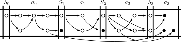
Figure 1: Example of an optimal schedule with proper separator for $m=2$ machines and makespan $12$. Sinks are solid black-filled circles, other jobs are white-filled. Sinks are processed only in $S_{1},S_{2},S_{3}$ and $\sigma_{3}$. Jobs in $\sigma_{i}$ are non-sinks that are successors of $S_{i}$ and not successors of $S_{i+1}$ ($i\in\{0,1,2\}$). In Subsection 3.1, we prove that such a decomposition exists for some optimal schedule.

As the jobs in $\sigma_{i}$ (for $i<\ell$) in the decomposition are determined by $S_{i}$ and $S_{i+1}$, the algorithm will recursively compute the makespan of such potential subschedules by considering all $n^{6}$ possible combinations. The existence of the decomposition ensures that there are no sinks in $\sigma_{0},\dots,\sigma_{\ell-1}$, so we make more progress when there are many sinks: Insight 1: If a subproblem has at least $\sqrt{n}$ sinks, then the number of jobs in its resulting subproblems decreases by $\Omega(\sqrt{n})$. To demonstrate that this insight is useful, consider a straightforward recursion. If each subproblem of the recursion contains at least $\sqrt{n}$ sinks, then the depth of the recursion is just $\mathcal{O}(\sqrt{n})$. Consequently, the size of the recursion tree can be bounded by $2^{\mathcal{O}(\sqrt{n}\log{n})}$.

To handle the case with few sinks, we use a different observation. Insight 2: There are $2^{\mathcal{O}(\sqrt{n}\log{n})}$ distinct subproblems generated with at most $\sqrt{n}$ sinks. This follows from the decomposition, as the subproblems generated by the recursion are uniquely described by the sets of sources and sinks within the associated precedence graph. Moreover, this graph has at most $3$ sources namely a set $S_{i}$ as implied by the properties of the decomposition. Leveraging this fact, we can utilize memorization to store the optimal makespan of these subproblems and solve them only once.

By combining Insights 1 and 2, we can employ a win-win strategy. We use a lookup table to handle subproblems with at most $\sqrt{n}$ sinks, and when a subproblem has more than $\sqrt{n}$ sinks, we make significant progress within each of the considered subproblems. This results in a branching tree of size $2^{\mathcal{O}(\sqrt{n}\log n)}$.

However, it is still highly nontrivial to see that we can output the optimal makespan based on the makespan of the $n^{6}$ created subproblems efficiently. We address this by showing that we can reconstruct the schedule in $n^{\mathcal{O}(m)}$ time with the assistance of dynamic programming. For this, we need the following crucial observation.

Insight 3: When computing the optimal makespan, based on the solutions of the subproblems, it is enough to keep track of one timeslot $S_{i}$ and the number of sinks that have been scheduled thus far.

The first part is a corollary of the properties of the decomposition. The second part of this observation relies on the fact that sinks are often interchangeable as they do not have successors. Therefore, it suffices to check whether the number of available sinks is at least the number of sinks scheduled thus far.

It should be noted that we can achieve the running time guaranteed by  Theorem 1.1 with an algorithm that follows more naturally from the decomposition of [16]. In particular, we can show that the algorithm from [16] augmented with a lookup table and an isomorphism check meets this requirement. However, the running time analysis of this alternative algorithm is more complicated than what is presented in this paper, so we opted to provide the current algorithm.

Unbounded number of machines.

When $m$ is given as input, the problem is known to be $\mathsf{NP}$-hard [36, 48], and the reduction from [36, 48] strongly indicates that $2^{o(n)}$ time algorithms are not possible: Any $2^{o(n)}$ algorithm for $P\,|\,\mathrm{prec},p_{j}=1|\,C_{\max}$ contradicts a plausible hypothesis about Densest $\kappa$-Subgraph [26] and implies a $2^{o(n)}$ time algorithm for the Biclique problem [32] on $n$-vertex graphs.

Natural dynamic programming over subsets7 of the jobs solves the problem in $\mathcal{O}^{\star}(2^{n}\binom{n}{m})$ time. An obvious question is whether this can be improved. It is conjectured that not all $\mathsf{NP}$-complete problems can be solved strictly faster than $\mathcal{O}^{\star}(2^{n})$ (where $n$ is some natural measure of the input size). The Strong Exponential Time Hypothesis (SETH) postulates that $k$-SAT cannot be solved in $\mathcal{O}(c^{n})$ time for any constant $c<2$. Breaking the $\mathcal{O}^{\star}(2^{n})$ barrier has been an active area of research in recent years, with results including algorithms with running times of $\mathcal{O}((2-\varepsilon)^{n})$ for Hamiltonian Cycle in undirected graphs [5], Bin Packing with a constant number of bins [41], and single machine scheduling with precedence constraints minimizing the total completion time [13]. We add $P\,|\,\mathrm{prec},p_{j}=1|\,C_{\max}$ problem to this list and show that it admits a faster than $\mathcal{O}^{\star}(2^{n})$ time algorithm, even when $m=\Theta(n)$ is given as input.

Theorem 1.2.

$P\,|\,\mathrm{prec},p_{j}=1|\,C_{\max}$ admits an $\mathcal{O}(1.997^{n})$ time algorithm.

Observe that for $m\leq\delta n$, Theorem 1.1 yields an $\mathcal{O}((2-\varepsilon)^{n})$ time algorithm (for some small constants $\varepsilon,\delta>0$). Theorem 1.2 is proved by combining this with an algorithm that runs in $\mathcal{O}^{\star}(2^{n-m})$ time. This algorithm improves over the mentioned $\mathcal{O}^{\star}(2^{n}\binom{n}{m})$ time algorithm by handling sinks more efficiently (of which we can assume there are at least $m$ with a reduction rule) and employing the subset convolution technique from [6] to avoid the $\binom{n}{m}$ term in the running time.

Related Work

Structured precedence graphs.

In this research line for the problem, $P\,|\,\mathrm{prec},p_{j}=1|\,C_{\max}$ is shown to be solvable in polynomial time for many structured inputs. Hu [31] gave a polynomial time algorithm when the precedence graph is a tree. This was later improved by Sethi [45], who showed that these instances can be solved in $\mathcal{O}(n)$ time. Garey et al. [23] considered a generalization when the precedence graph is an opposing forest, i.e., the disjoint union of an in-forest and out-forest. They showed that the problem is $\mathsf{NP}$-hard when $m$ is given as an input, and that the problem can be solved in polynomial time when $m$ is a fixed constant. Papadimitriou and Yannakakis [43] gave an $\mathcal{O}(n+m)$ time algorithm when the precedence graph is an interval order. Fujii et al. [19] presented the first polynomial time algorithm when $m=2$. Later, Coffman and Graham [12] gave an alternative $\mathcal{O}(n^{2})$ time algorithm for two machines. The running time was later improved to near-linear by Gabow [20] and finally to truly linear by Gabow and Tarjan [21]. For a more detailed overview and other variants of $P\,|\,\mathrm{prec},p_{j}=1|\,C_{\max}$ , see the survey of Lawler et al. [35].

Exponential time algorithms.

Scheduling problems have been extensively studied from the perspective of exact algorithms, especially in the last decade. From the point of view of parameterized complexity, the natural parameter for $P\,|\,\mathrm{prec},p_{j}=1|\,C_{\max}$ is the number of machines, $m$. Bodlaender and Fellows [8] show that problem is $\mathsf{W[2]}$-hard parameterized by $m$. Recently, Bodlaender et al. [9] showed that $P\,|\,\mathrm{prec},p_{j}=1|\,C_{\max}$ parameterized by $m$ is $\mathsf{XNLP}$-hard, which implies $\mathsf{W[t]}$-hardness for every $t$. These results imply that it is highly unlikely that $P\,|\,\mathrm{prec},p_{j}=1|\,C_{\max}$ can be solved in $f(m)n^{\mathcal{O}(1)}$ for any function $f$. A work that is very important for this paper is by Dolev and Warmuth [16], who show that the problem can be solved in time $\mathcal{O}(n^{h(m-1)+1})$, where $h$ is the cardinality of the longest chain in the precedence graph. Several other parameterizations have been studied, such as the maximum cardinality of an antichain in the precedence graph. We refer to a survey by Mnich and van Bevern [40].

Lower bounds conditioned on the Exponential Time Hypothesis are given (among others) by Chen et al. in [11]. T’kindt et al. give a survey on moderately exponential time algorithms for scheduling problems [47]. Cygan et al. [13] gave an $\mathcal{O}((2-\varepsilon)^{n})$ time algorithm (for some constant $\varepsilon>0$) for the problem of scheduling jobs of arbitrary length with precedence constraints on one machine.

Approximation.

The $P\,|\,\mathrm{prec},p_{j}=1|\,C_{\max}$ problem has been extensively studied through the lens of approximation algorithms, where the aim is to approximate the makespan. A classic result by Graham [27] gives a polynomial time $(2-1/m)$-approximation, and Svensson [46] showed hardness for improving this for large $m$. In a breakthrough, Levey and Rothvoß [37] give a $(1+\varepsilon)$-approximation in $\exp\left(\exp\left(\mathcal{O}(\frac{m^{2}}{\varepsilon^{2}}\log^{2}\log n)\right)\right)$ time. This strongly indicates that the problem is not $\mathsf{APX}$-hard for constant $m$. This was subsequently improved by [24] and simplified in [14]. The currently fastest algorithm is due to Li [38] who improved the running time to $n^{\mathcal{O}\left(\frac{m^{4}}{\varepsilon^{3}}\log^{3}\log(n)\right)}$. Note that the dependence on $\varepsilon$ in these algorithms is prohibitively high if one wants to solve the problem exactly. To do so, one would need to set $\varepsilon=\mathcal{O}(1/n)$, yielding an exponential time algorithm. A prominent open question is to give a PTAS even when the number of machines is fixed (see the recent survey of Bansal [4]). In [37] it was called a tantalizing open question whether there are similar results for $P3\,|\,\mathrm{prec}|\,C_{\max}$.

There are some interesting similarities between this research line and our work: In both the maximum chain length plays an important role, and a crucial insight is that there is always an (approximately) optimal solution with structured decomposition. Yet, of course, approximation schemes do not guarantee subexponential time algorithms. For example, in contrast to the aforementioned question by [37], it is highly unlikely that even $P2\,|\,\mathrm{prec},p_{j}=\{1,2\}|\,C_{\max}$ has a $2^{o(n)}$ time algorithm: This follows from the reduction by Ullman [48] to $P\,|\,\mathrm{prec},p_{j}=1|\,C_{\max}$ .

Organization

In Section 2 we include preliminaries. In Subsection 3.1 we present the decomposition and the algorithm of Dolev and Warmuth [16]. In Section 4 we prove Theorem 1.1 and in Section 5 we prove Theorem 1.2. Section 6 contains the conclusion and further research directions. Appendix A contains a conditional lower bound on $Pm\,|\,\mathrm{prec},p_{j}=1|\,C_{\max}$ .

2 Preliminaries

We use $\mathcal{O}^{\star}(\cdot)$ notation to hide polynomial factors in the input size. Throughout the paper, we use $\binom{n}{\leq k}\coloneqq\sum_{i=0}^{k}\binom{n}{i}$ shorthand notation. We often use $n$ as the number of jobs in the input and $m$ as the number of machines.

The set of precedence constraints is represented with a directed acyclic graph $G=(V,A)$, referred to as the precedence graph. We will interchangeably use the notations for arcs in $G$ and the partial order, i.e., $(v,w)\in A$ if and only if $v\prec w$. Similarly, we use the name jobs to refer to the vertices of $G$. Note that we assume that $G$ is the transitive closure of itself, i.e. if $u\prec v$ and $v\prec w$ then $u\prec w$.

A set $X\subseteq V$ of jobs is called a chain if all jobs in $X$ are comparable to each other. Alternatively, if all jobs in $X$ are incomparable to each other, $X$ is called an antichain. For a job $v$, we denote

$${\textsf{pred}}(v) \coloneqq\{u:u\prec v\}, \qquad{\textsf{pred}}[v] \coloneqq{\textsf{pred}}(v)\cup\{v\},$$

$${{\textsf{succ}}}(v) \coloneqq\{u:v\prec u\}, \qquad{{\textsf{succ}}}[v] \coloneqq{{\textsf{succ}}}(v)\cup\{v\},$$

as the sets of all predecessors and respectively successors of $$v X$$. For a set of jobs we let

$${\textsf{pred}}(X) \coloneqq\bigcup_{v\in X}{\textsf{pred}}(v), \qquad{{\textsf{succ}}}(X) \coloneqq\bigcup_{v\in X}{{\textsf{succ}}}(v),$$

$${\textsf{pred}}[X] \coloneqq{\textsf{pred}}(X)\cup X, \qquad{{\textsf{succ}}}[X] \coloneqq{{\textsf{succ}}}(X)\cup X.$$

We refer to a job that does not have any predecessor as a source, and we say that a job that does not have any successors is a sink. We use ${{\textsf{sinks}}}(G)$ to refer to the set of all sinks in $G$.

A schedule is a sequence $(T_{1},\ldots,T_{M})$ of pairwise disjoint sets $T_{1},\ldots,T_{M}\subseteq V$ that we will refer to as timeslots. Consider $X\subseteq V$ such that for all $v,w,x\in V$, we have that $v\prec w\prec x$ and $v,x\in X$ implies $w\in X$. We say that $(T_{1},\ldots,T_{M})$ is a feasible schedule for the set $X$ if (i) $\bigcup_{i=1}^{M}T_{i}=X$, (ii) $|T_{i}|\leq m$ for every $i\in\{1,\dots,M\}$, and (iii) if $u\in T_{i}$, $v\in T_{j}$, and $u\in{\textsf{pred}}(v)$, then $i<j$. We say that such a schedule has makespan $M$. Sometimes, we omit the set $X$ in the definition of a feasible schedule when we simply mean a feasible schedule for all jobs $V$. For a schedule $\sigma$, we use $|\sigma|$ to denote its makespan and $V(\sigma)$ to denote the set of jobs in the schedule. To concatenate two schedules, we use the $\oplus$ operator, where $(T_{1},\ldots,T_{\ell})\oplus(T_{\ell+1},\ldots,T_{k})=(T_{1},\ldots,T_{k})$. Note that we treat a single timeslot as a schedule itself, therefore $(T_{1},\ldots,T_{\ell})\oplus T_{\ell+1}=(T_{1},\ldots,T_{\ell+1})$.

3 Decomposing the Schedule

Now, we prove there is an optimal schedule that can be decomposed in a certain way, and in Subsection 3.2, we show how an optimal schedule with such a decomposition can be found given the solutions to certain subproblems.

3.1 Proper Separator

Now, we formally define a proper separator of a schedule. We stress that this decomposition is an extension of the decomposition in [16] known under the name of zero-adjusted schedule.

Definition 3.1 (Proper Separator).

Given a precedence graph $G$ with at most $m$ sources $S_{0}$ and a feasible schedule $\sigma$. We say that sets $S_{1},\ldots,S_{\ell}\subseteq V(G)$ form a separator of $\sigma$ if $\sigma$ can be written as:

$$\sigma=\left(S_{0}\oplus\sigma_{0}\oplus S_{1}\oplus\sigma_{1}\oplus S_{2}\oplus\ldots\oplus S_{\ell}\oplus\sigma_{\ell}\right),$$

where $\sigma_{i}$ is a feasible schedule for $V(\sigma_{i})$ for all $i\in\{0,\dots,\ell\}$. We will say that separator $S_{1},\ldots,S_{\ell}$ of $\sigma$ is proper if all of the following conditions hold:

1. $V(\sigma_{i})={{\textsf{succ}}}(S_{i})\setminus({{\textsf{succ}}}[S_{i+1}]\cup{{\textsf{sinks}}}(G))$ for all $i\in\{0,\dots,\ell-1\}$,

2. $S_{j}\subseteq{{\textsf{succ}}}(S_{i})\cup{{\textsf{sinks}}}(G)$ for all $0\leq i<j\leq\ell$,

3. $V(\sigma_{\ell})\subseteq{{\textsf{sinks}}}(G)$.

Note that the assumption on the number of sources is mild and only for notational convenience. The power of this decomposition lies in the fact that, given the input graph $G$, the jobs in $\sigma_{i}$ are completely determined by sets $S_{i}$ and $S_{i+1}$, both of size at most $m$.

Theorem 3.2.

For any precedence graph $G$ with at most $m$ sources, there is a schedule of minimum makespan with a proper separator.

Proof.

Consider a feasible schedule $\sigma=(T_{1},\ldots,T_{M})$ of minimum makespan. Since $|S_{0}|\leq m$, we may assume $T_{1}=S_{0}$ because $T_{1}$ is the first timeslot, and it can only contain sources. We introduce the definition of a conflict. This definition is designed so that a non-sink can be moved to an earlier timeslot in the schedule if there is a conflict.

Definition 3.3 (Conflict).

We say that a non-sink $v\in V(G)\setminus{{\textsf{sinks}}}(G)$ and a timeslot $T_{i}$ are in conflict if (a) $v\in T_{j}$ with $j>i$, (b) ${\textsf{pred}}(v)\subseteq T_{1}\cup\ldots\cup T_{i-1}$, and (c) $|T_{i}\setminus{{\textsf{sinks}}}(G)|<m$.

Procedure Resolve-Conflicts.

The iterative procedure Resolve-Conflicts modifies $\sigma$ as follows: while there exists some timeslot $T_{i}$ and job $v$ that are in conflict, we move $v$ to $T_{i}$. If $|T_{i}|<m$, then there is an unused slot in $T_{i}$ and we can freely move $v$ to $T_{i}$. Otherwise, $T_{i}$ contains some sink $s\in T_{i}\cap{{\textsf{sinks}}}(G)$. In that case, we swap $s$ and $v$ in $\sigma$, i.e., we move $v$ to timeslot $T_{i}$ and $s$ to timeslot $T_{j}$.

Every time Resolve-Conflicts finds a conflict, it moves a non-sink to an earlier timeslot, and only sinks are moved to later timeslots. Since there are at most $n$ non-sinks and $M$ timeslots, Resolve-Conflicts must therefore halt after at most $nM$ iterations. Note that Resolve-Conflicts only modifies timeslots of the original schedule and does not add any new ones to $\sigma$. Therefore, the makespan does not increase.

Feasibility.

Consider a schedule $\sigma=(T_{1},\ldots,T_{M})$ at some iteration and schedule $\sigma^{\prime}$ after resolving the conflicting $v$ and $T_{i}$. By the construction, each timeslot in $\sigma^{\prime}$ has size $\leq m$. Therefore it remains to show that precedence constraints are preserved. Only job $v$ and possibly a sink $s$ change their positions. Hence we only need to check their precedence constraints.

Job $s$ is a sink in the timeslot $T_{i}$ of $\sigma$, hence the predecessors of $s$ are scheduled before timeslot $i$. Since $s$ is a sink and has no successors, moving it to a later timeslot preserves its precedence constraints. For job $v$, it satisfies property (b), which means that all its predecessors are scheduled strictly before timeslot $T_{i}$. Therefore, scheduling $v$ at timeslot $T_{i}$ does not violate its precedence constraints. Additionally, the successors of job $v$ are still valid because $v$ is moved to an earlier timeslot. Thus, the modified schedule $\sigma^{\prime}$ is feasible.

Resolve-Conflicts returns a schedule with a proper separator.

Note that after the modification we still have $T_{1}=S_{0}$: The first timeslot is never in conflict with any job because of property (b), and $T_{1}$ initially contains all sources. We construct the proper separator $S_{1},\ldots,S_{\ell}$ for $\sigma$ as follows: Let $t$ be the smallest integer such that after time $t$, only jobs from ${{\textsf{sinks}}}(G)$ are scheduled. We choose $S_{1},\ldots,S_{\ell-1}$ to be all timeslots (in order) in $\sigma$ before $t$ with $|S_{i}\setminus{{\textsf{sinks}}}(G)|<m$. Finally, we let $S_{\ell}$ be the set of jobs scheduled at $t$. Observe that this way we can decompose $\sigma$ to be

$$\sigma=\left(S_{0}\oplus\sigma_{0}\oplus S_{1}\oplus\sigma_{1}\oplus S_{2}\oplus\ldots\oplus S_{\ell}\oplus\sigma_{\ell}\right),$$

such that $V(\sigma_{j})\subseteq V(G)\setminus{{\textsf{sinks}}}(G)$ for all $j\in\{0,\ldots,\ell-1\}$ and $V(\sigma_{\ell})\subseteq{{\textsf{sinks}}}(G)$. By construction $V(\sigma_{\ell})\subseteq{{\textsf{sinks}}}(G)$ and (C) is satisfied.

It remains to establish (A) and (B). Here, we crucially use the assumption that schedule $\sigma$ has no conflicts. In particular, timeslots $S_{1},\ldots,S_{\ell}$ are not in conflict with any job $v\in V(G)\setminus{{\textsf{sinks}}}(G)$.

For property (A), observe that by the construction $V(\sigma_{i})\cap{{\textsf{sinks}}}(G)=\emptyset$ for every $i\in\{0,\ldots,\ell-1\}$. So we only need to argue about non-sinks.

First we show $v\in V(\sigma_{i})$ implies $v\in{{\textsf{succ}}}(S_{i})\setminus({{\textsf{succ}}}[S_{i+1}]\cup{{\textsf{sinks}}}(G))$. Clearly, $v\not\in{{\textsf{succ}}}[S_{i+1}]$ as $\sigma$ is feasible and $v$ is processed before $S_{i+1}$. Moreover, $v\in{{\textsf{succ}}}(S_{i})$, otherwise take $v$ as the earliest job of $\sigma_{i}$ not in ${{\textsf{succ}}}(S_{i})$, then $S_{i}$ and $v$ are in conflict, contradicting the assumption that $\sigma$ has no conflicts.

For the other direction, we show that $v\not\in V(\sigma_{i})$ implies $v\not\in{{\textsf{succ}}}(S_{i})\setminus({{\textsf{succ}}}[S_{i+1}]\cup{{\textsf{sinks}}}(G))$. If a job $v$ is before $\sigma_{i}$ in schedule $\sigma$, then $v$ cannot be in ${{\textsf{succ}}}(S_{i})$ as $\sigma$ is feasible. Finally, if there is a non-sink scheduled after $\sigma_{i}$ that is additionally not in ${{\textsf{succ}}}[S_{i+1}]$, then take $v$ as the earliest such job. Now, $S_{i+1}$ and $v$ are in conflict, contradicting the assumption that $\sigma$ has no conflicts.

It remains to establish property (B). For the sake of contradiction, take job $v\in S_{j}\setminus{{\textsf{sinks}}}(G)$ such that $v\not\in{{\textsf{succ}}}(S_{i})$ for some $i<j$. If all ${\textsf{pred}}(v)$ are scheduled before $S_{i}$ then $v$ and $S_{i}$ are in conflict. Therefore, there exists $v^{\prime}\in{\textsf{pred}}(v)$ that is scheduled after $S_{i}$. Take $v^{\prime}$ to be the earliest such predecessor of $v$. But then all predecessors of $v^{\prime}$ must be scheduled before $S_{i}$. This means that $v^{\prime}$ and $S_{i}$ are in conflict, contradicting that $\sigma$ has no conflicts.

Concluding, Resolve-Conflicts turns any schedule into a schedule with a proper separator without increasing the makespan. This concludes the proof. ∎

3.2 Reconstructing the Schedule

In this subsection, we will show how to reconstruct an optimal schedule for a graph $G$ with at most $m$ sources $S_{0}$, given a set of so-called subschedules. Note that we can assume that an optimal schedule $\sigma^{\star}$ for $G$ exists that admits a proper separator, by Theorem 3.2. Hence, $\sigma^{\star}$ can be written as

$$\sigma^{\star}=\left(S_{0}\oplus\sigma^{\star}_{0}\oplus S^{\star}_{1}\oplus\sigma^{\star}_{1}\oplus\ldots\oplus S^{\star}_{\ell}\oplus\sigma^{\star}_{\ell}\right),$$

such that the three conditions in Definition 3.1 hold. To reconstruct the schedule we will use a dynamic programming table to construct such a schedule. For this purpose, we define a partial proper schedule as a schedule for a subset of $V(G)$ of the form $(S_{0}\oplus\sigma_{0}\oplus S_{1}\oplus\sigma_{1}\oplus\ldots\oplus\sigma_{q-1}\oplus S_{q})$ such that the first two conditions of Definition 3.1 hold:

1. $V(\sigma_{i})={{\textsf{succ}}}(S_{i})\setminus({{\textsf{succ}}}[S_{i+1}]\cup{{\textsf{sinks}}}(G))$ for all $0\leq i<q$,

2. $S_{j}\subseteq{{\textsf{succ}}}(S_{i})\cup{{\textsf{sinks}}}(G)$ for all $0\leq i<j\leq q$.

In our algorithm, we will compute the minimum makespan for all possible $\sigma_{i}$’s. Such schedules are formally defined as follows.

Definition 3.4 (Subschedule).

For a graph $G$ and slots $A,B\subseteq V(G)$ with $|A|,|B|\leq m$ we say that $\sigma[A,B]$ is a subschedule if it is an optimal schedule of jobs $V(\sigma[A,B])$ and

$$V(\sigma[A,B])={{\textsf{succ}}}(A)\setminus({{\textsf{succ}}}[B]\cup{{\textsf{sinks}}}(G)).$$

Intuitively the set of jobs in a partial proper schedule is fully determined by the set $S_{q}$ up to the jobs from ${{\textsf{sinks}}}(G)$. We prove this formally in the following claim.

Claim 3.5.

Let $\sigma=(S_{0}\oplus\sigma_{0}\oplus S_{1}\oplus\sigma_{1}\oplus\ldots\oplus\sigma_{q-1}\oplus S_{q})$ be a partial proper schedule. Then

$$V(\sigma)\setminus{{\textsf{sinks}}}(G)=V(G)\setminus({{\textsf{succ}}}(S_{q})\cup{{\textsf{sinks}}}(G)).$$

Proof. By definition of $V(\sigma)\setminus{{\textsf{sinks}}}(G)$ is equal to $\left(S_{0}\cup\bigcup_{i=0}^{q-1}\left(S_{i+1}\cup V(\sigma_{i})\right)\right)\setminus{{\textsf{sinks}}}(G)$. Then, we invoke the property (A’) and get that left-hand side is equal to:

$$\left(S_{0}\cup\bigcup_{i=0}^{q-1}\left(S_{i+1}\cup({{\textsf{succ}}}(S_{i})\setminus({{\textsf{succ}}}[S_{i+1}]\cup{{\textsf{sinks}}}(G)))\right)\right)\setminus{{\textsf{sinks}}}(G).$$

Note, that this can be simplified to $\left(S_{0}\cup\bigcup_{i=0}^{q-1}\left({{\textsf{succ}}}(S_{i})\setminus{{\textsf{succ}}}(S_{i+1})\right)\right)\setminus{{\textsf{sinks}}}(G)$. Next, we use property (B’) and the sum telescopes to $(S_{0}\cup({{\textsf{succ}}}(S_{0})\setminus{{\textsf{succ}}}(S_{q})))\setminus{{\textsf{sinks}}}(G)$ which is equal to $V(G)\setminus({{\textsf{succ}}}(S_{q})\cup{{\textsf{sinks}}}(G))$ because $S_{0}$ are all the sources. $\blacksquare$

We are now ready to state and prove the correctness of our reconstruction algorithm.

Lemma 3.6.

There is an algorithm reconstruct that given a precedence graph $G$ with $n$ jobs and at most $m$ sources, and the following set of subschedules $\{\sigma[X,Y]\mid\text{ antichains }X,Y\subseteq V(G)\text{ with }X\subseteq{{\textsf{succ}}}(Y)$ and $|X|,|Y|\leq m\}$, outputs the minimum makespan of a schedule for $G$ in $\binom{n}{\leq 2m}\cdot n^{\mathcal{O}(1)}$ time.

Proof.

Assume $n>0$, as otherwise we output that the makespan is $0$. Let $S_{0}$ be the set of sources of $G$. We define a set of possible separator slots:

$${{\textsf{SepSlots}}}\coloneqq\{X\subseteq V(G)\setminus{{\textsf{sinks}}}(G)\text{ such that }|X|\leq m\text{ and }X\text{ is an antichain}\}.$$

Note that $S_{0}\setminus{{\textsf{sinks}}}(G),S_{1}\setminus{{\textsf{sinks}}}(G),\dots,S_{\ell}\setminus{{\textsf{sinks}}}(G)$ are all in SepSlots.

Definition of dynamic programming table.

For any $k\in\mathbb{N}$ and $X\in{{\textsf{SepSlots}}}$ we let

$$\mathsf{DP}[X,k]\coloneqq\min\{ \text{ makespan of partial proper schedule }\sigma=(S_{0}\oplus\sigma_{0}\oplus S_{1}\oplus\sigma_{1}\oplus\ldots\oplus\sigma_{q-1}\oplus S_{q}):$$

$$|V(\sigma)\cap{{\textsf{sinks}}}(G)|=k,X=S_{q}\setminus{{\textsf{sinks}}}(G)\}.$$

In other words, $\mathsf{DP}[X,k]$ tells us the minimum makespan of a partial proper schedule for $V(G)\setminus({{\textsf{succ}}}(X)\cup{{\textsf{sinks}}}(G))$ (because of 3.5) and $k$ jobs of ${{\textsf{sinks}}}(G)$, such that all jobs from $X$ (and possibly some sinks) are processed at the last timeslot. At the end, after each entry of $\mathsf{DP}[X,k]$ is computed, the minimum makespan of a schedule for $G$ is then equal to

$$\min_{\begin{subarray}{c}X\in{{\textsf{SepSlots}}},\\ {{\textsf{succ}}}(X)\subseteq{{\textsf{sinks}}}(G),\\ k\leq|{{\textsf{sinks}}}(G)|\end{subarray}}\left\{\mathsf{DP}[X,|{{\textsf{sinks}}}(G)|-k]+\left\lceil\frac{k}{m}\right\rceil\right\}.$$

To see that this is correct, recall that $\sigma^{\star}_{\ell}$ only contains jobs from ${{\textsf{sinks}}}(G)$, which can be processed in any order. Hence, we search for a partial proper schedule processing all jobs, except for $k$ jobs from ${{\textsf{sinks}}}(G)$ (hence ${{\textsf{succ}}}(X)\subseteq{{\textsf{sinks}}}(G)$ using 3.5), and we add the time needed to process the $k$ remaining jobs from ${{\textsf{sinks}}}(G)$ in any order.

Base-case.

In order to process $k$ jobs from ${{\textsf{sinks}}}(G)$, all of their predecessors must be completed. In particular, we demand for each such sink that its predecessors are processed before the last timeslot. Hence, we set

$$\mathsf{DP}[X,k] =\infty\;\;\text{ if }|\{v\in{{\textsf{sinks}}}(G)\mid{\textsf{pred}}(v)\subseteq V(G)\setminus{{\textsf{succ}}}[X]\}|<k.$$

Moreover, for any $$X\in{{\textsf{SepSlots}}} X\cap S_{0}\not=\emptyset$$ such that we set:

$$\mathsf{DP}[X,k] =\begin{cases}1&\text{if }X=S_{0}\setminus{{\textsf{sinks}}}(G)\text{ and }S_{0}\cap{{\textsf{sinks}}}(G)=k,\\ \infty&\text{otherwise.}\end{cases}$$

For the correctness of this case, note that $X$ contains sources and the number of sources is assumed to be at most $m$. Therefore, in the optimal schedule, these sources must be scheduled in the first moment, i.e., $\sigma=(S_{0})$. Hence, if $X\cap S_{0}\neq\emptyset$ then it must hold that $X=S_{0}\setminus{{\textsf{sinks}}}(G)$. We also need to check that exactly $k$ sinks are scheduled, so $|S_{0}\cap{{\textsf{sinks}}}(G)|=k$ must hold.

Recursive formula.

To compute the remaining values of the $\mathsf{DP}$ table we use the following recursive formula:

$$\mathsf{DP}[X,k]=\min_{\begin{subarray}{c}Y\in{{\textsf{SepSlots}}},\\ X\subseteq{{\textsf{succ}}}(Y),\\ k^{\prime}\leq m-|X|\end{subarray}}\{\mathsf{DP}[Y,k-k^{\prime}]+|\sigma[Y,X]|+1\}.$$

Observe that each $|\sigma[Y,X]|$ is given as the input to the algorithm. It remains to prove that this recurrence is correct. The strategy is to show that the left-hand side is $\leq$ and $\geq$ to the right-hand side. We prove this by the induction over $k$ and consecutive timeslots in the separator (i.e., we prove it to be true for $A$ before $B$ if $B\subseteq{{\textsf{succ}}}(A)$).

Direction ($\geq$):

Let $\mathsf{DP}[X,k]=M$, i.e., there is a partial proper schedule $\sigma=(S_{0}\oplus\sigma_{0}\oplus\ldots\oplus\sigma_{q-1}\oplus S_{q})$ of makespan $M$ such that $|V(\sigma)\cap{{\textsf{sinks}}}(G)|=k$ and $X=S_{q}\setminus{{\textsf{sinks}}}(G)$. Take $Y\coloneqq S_{q-1}\setminus{{\textsf{sinks}}}(G)$. By condition (B’), $S_{q}\subseteq{{\textsf{succ}}}(S_{q-1})\cup{{\textsf{sinks}}}(G)$, and so $X=S_{q}\setminus{{\textsf{sinks}}}(G)\subseteq{{\textsf{succ}}}(Y)$, so $Y$ is one of the sets considered in the recursive formula. Take $k^{\prime}\coloneqq|S_{q}\cap{{\textsf{sinks}}}(G)|$. We will show that $M\geq\mathsf{DP}[Y,k-k^{\prime}]+|\sigma[Y,X]|+1$. Note that $\sigma^{\prime}=(S_{0}\oplus\sigma_{0}\oplus\ldots\oplus\sigma_{q-2}\oplus S_{q-1})$ is a partial proper schedule, as conditions (A’) and (B’) still hold. Moreover, because of condition (A’), $\sigma_{q-1}\cap{{\textsf{sinks}}}(G)=\emptyset$, so $\sigma^{\prime}$ contains $k-k^{\prime}$ jobs from ${{\textsf{sinks}}}(G)$. Lastly, by definition, $Y=S_{q-1}\setminus{{\textsf{sinks}}}(G)$, hence $\sigma^{\prime}$ is a partial proper schedule proving that $\mathsf{DP}[Y,k-k^{\prime}]\leq|\sigma^{\prime}|$. We know by condition (A’) that $V(\sigma_{q-1})={{\textsf{succ}}}(S_{q-1})\setminus({{\textsf{succ}}}[S_{q}]\cup{{\textsf{sinks}}}(G))={{\textsf{succ}}}(Y)\setminus({{\textsf{succ}}}[X]\cup{{\textsf{sinks}}}(G))$ (as both $X$ and $Y$ do not contain any sinks), hence $|\sigma_{q-1}|\geq|\sigma[Y,X]|$. We conclude that $M=|\sigma^{\prime}|+|\sigma_{q-1}|+1\geq\mathsf{DP}[Y,k-k^{\prime}]+|\sigma[Y,X]|+1$.

Direction ($\leq$):

Let $M=\mathsf{DP}[Y,k-k^{\prime}]+\sigma[Y,X]+1$ for some $Y\in{{\textsf{SepSlots}}}$, $X\subseteq{{\textsf{succ}}}(Y)$, and $k^{\prime}\leq m-|X|$. By induction, we have a partial proper schedule $\sigma^{\prime}=(S_{0}\oplus\sigma_{0}\oplus\ldots\oplus\sigma_{q-2}\oplus S_{q-1})$ with a makespan $\mathsf{DP}[Y,k-k^{\prime}]$ for $V(G)\setminus({{\textsf{succ}}}(Y)\cup{{\textsf{sinks}}}(G))$ and $k-k^{\prime}$ jobs from ${{\textsf{sinks}}}(G)$ such that $S_{q-1}\setminus{{\textsf{sinks}}}(G)=Y$. Let $Z\coloneqq V(\sigma^{\prime})\cap{{\textsf{sinks}}}(G)$ be the $k-k^{\prime}$ sinks that are in $\sigma^{\prime}$. Then let $Z^{\prime}\subseteq\{v\in{{\textsf{sinks}}}(G)\mid{\textsf{pred}}(v)\subseteq V(G)\setminus{{\textsf{succ}}}[X]\}\setminus Z$ such that $|Z^{\prime}|=k^{\prime}$. We can choose $Z^{\prime}$ in such a way because we set $\mathsf{DP}[X,k]=\infty$ if $|\{v\in{{\textsf{sinks}}}(G)\mid{\textsf{pred}}(v)\subseteq V(G)\setminus{{\textsf{succ}}}[X]\}|<k$.

We show that $\sigma=(\sigma^{\prime}\oplus\sigma[Y,X]\oplus(X\cup Z))$ is a partial proper schedule. First, note that the precedence constraints in $\sigma$ are satisfied: all jobs in $\sigma[Y,X]$ are successors of $S_{q-1}$; for all sinks in $Z$, their processors are finished before the last timeslot by definition, and none of the successors of $X$ are in $\sigma$. Condition (A’) holds for $\sigma^{\prime}$, so it remains to check (A’) for $\sigma[Y,X]$: $V(\sigma[Y,X])={{\textsf{succ}}}(Y)\setminus({{\textsf{succ}}}[X]\cup{{\textsf{sinks}}}(G))$ by definition of subschedule, and so condition (A’) holds. Similarly, we only need to verify condition (B’) for $S_{q}=(X\cup Z)$. By the choice of $Y$, $X\subseteq{{\textsf{succ}}}(Y)$; hence, $S_{q}\subseteq{{\textsf{succ}}}(S_{q-1})\cup{{\textsf{sinks}}}(G)$. As $\sigma^{\prime}$ is a partial proper schedule, we have that $S_{q-1}\subseteq{{\textsf{succ}}}(S_{i})\cup{{\textsf{sinks}}}(G)$ for all $i<q-1$. Therefore, $S_{q}\subseteq{{\textsf{succ}}}(S_{i})\cup{{\textsf{sinks}}}(G)$ for all $i<q$. So $\sigma$ is a partial proper schedule with $|V(\sigma)\cap{{\textsf{sinks}}}(G)|=k$, $X=S_{q}\setminus{{\textsf{sinks}}}(G)$, and it has makespan $M$. Hence, we conclude $\mathsf{DP}[X,k]\leq M$.

Running time.

We are left to analyze the running time of this algorithm. Naively, there are at most $|{{\textsf{SepSlots}}}|\cdot n$ table entries, and each table entry $\mathsf{DP}[\cdot,\cdot]$ can be computed in $\mathcal{O}(|{{\textsf{SepSlots}}}|\cdot m)$ time, in total giving a running time of $\binom{n}{\leq m}^{2}\cdot n^{\mathcal{O}(1)}$. However, to compute a table entry $\mathsf{DP}[X,k]$, we only use table entries $\mathsf{DP}[Y,k^{\prime}]$ where $X\subseteq{{\textsf{succ}}}(Y)$ and both $X$ and $Y$ are antichains. Moreover, the combination of jobs from $X$ and $Y$ only appears once: given a set $X\cup Y$, one can determine what is $X$ by taking all jobs that have some predecessor in $X\cup Y$. Therefore, the running time can be bounded by $\binom{n}{\leq 2m}\cdot n^{\mathcal{O}(1)}$ because $|X\cup Y|\leq 2m$. ∎

4 Subexponential Time Algorithm

In this section, we prove Theorem 1. Before we present the algorithm, we introduce the notion of an interval of graph $G$ that will essentially correspond to the subproblems in our algorithm.

Interval and new sinks.

For every two antichains $A,B\subseteq V(G)$ with $B\subseteq{{\textsf{succ}}}(A)$ the intervals of $G$ are defined as

$$\mathrm{Int}(A,B]\coloneqq G[{{\textsf{succ}}}(A)\cap{\textsf{pred}}[B]],\qquad\mathrm{Int}[A,B]\coloneqq G[{{\textsf{succ}}}[A]\cap{\textsf{pred}}[B]].$$

It follows from the fact that $B$ is an antichain that $B={{\textsf{sinks}}}(\mathrm{Int}(A,B])$. Our algorithm schedules $\mathrm{Int}(A,B]$ recursively. Therefore, at the beginning of the algorithm, we create a super-source by adding a single job $s_{0}$ and making it the source of every job in $V(G)$. Note that $G=\mathrm{Int}({s_{0}},{{\textsf{sinks}}}(G)]$, which serves as the starting point for our algorithm (see Fig. 2 for an illustration of an interval).

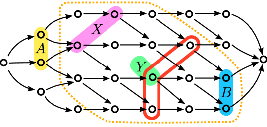
Figure 2: Yellow-highlighted jobs are in $A$, blue-highlighted jobs are in $B$, and the dotted region shows jobs in $\mathrm{Int}(A,B]$. For the definition of $\mathsf{NewSinks}(X,Y)$, purple-highlighted jobs are in $X$ and a single green-highlighted job is in $Y$. The three jobs of $\mathsf{NewSinks}(X,Y)$ are inside the red border.

Fix an interval $\mathrm{Int}(A,B]$. The set of jobs that need to be scheduled is simply the set of jobs in the current interval, i.e., $\mathsf{Jobs}={{\textsf{succ}}}(A)\cap{\textsf{pred}}[B]$. We show how to decompose $\mathrm{Int}(A,B]$ into subproblems. To that end, we consider all antichains $X,Y\subseteq\mathsf{Jobs}$ such that $Y\subseteq{{\textsf{succ}}}(X)$ and $|Y|,|X|\leq m$. For each such pair $X,Y$ and for $\mathsf{Jobs}$, we define the sinks of the new subproblems as follows:

$$\mathsf{NewSinks}(X,Y)\coloneqq{{\textsf{sinks}}}(G[\mathsf{Jobs}\cap{{\textsf{succ}}}(X)\setminus({{\textsf{succ}}}(Y)\cup B)]).$$

See Fig. 2 for an illustration of the definition of $\mathsf{NewSinks}$.

Algorithm.

We now present the algorithm behind Theorem 1.1 (see Algorithm 1). For any set $A,B\subseteq V(G)$, the subroutine $\mathsf{schedule}(A,B)$ computes the minimum makespan of the schedule of the graph $\mathrm{Int}(A,B]$. We will maintain the invariant that $B\subseteq{{\textsf{succ}}}(A)$ in each call to $\mathsf{schedule}(A,B)$ so that $\mathrm{Int}(A,B]$ is correctly defined. At the beginning of the subroutine, we check (using an additional look-up table) whether the solution to $\mathsf{schedule}(A,B)$ has already been computed. If so, we return it. Next, we compute the set of jobs of $\mathrm{Int}(A,B]$ and store it as $\mathsf{Jobs}\coloneqq{{\textsf{succ}}}(A)\cap{\textsf{pred}}[B]$. Then, we check the base-case, defined as $\mathsf{Jobs}=\emptyset$. In this case, the makespan is $0$ as there are no jobs to be scheduled.

In the remaining case, we have $\mathsf{Jobs}\neq\emptyset$. Then we iterate over every possible pair of slots, i.e., antichains $X,Y\subseteq\mathsf{Jobs}$ with $|X|$ and $|Y|$ of size at most $m$ and $Y\subseteq{{\textsf{succ}}}(X)$. The hope is that $X$ and $Y$ are consecutive slots of a proper separator for the optimal schedule for $\mathrm{Int}[A,B]$. To compute the minimum makespan of the subschedule related to $X$ and $Y$, we ask for the minimum makespan for the graph $\mathrm{Int}(X,\mathsf{NewSinks}(X,Y)]$ for every admissible $X,Y$ and collect all answers.

After the answer to each of the subschedules is computed, we combine them using Lemma 3.6 and return the minimum makespan of the schedule for the graph $\mathrm{Int}[A,B]$. Finally, we subtract $1$ from the makespan returned by Lemma 3.6 to account for the fact that $\mathrm{Int}(A,B]$ is the graph $\mathrm{Int}[A,B]$ without sources $A$ (and these sources are always scheduled at the first moment).

1 function $\mathsf{schedule}(A,B)$:

2 return answer if $\mathsf{schedule}(A,B)$ was already computed

3  // Check lookup-table

4 $\mathsf{Jobs}\coloneqq{{\textsf{succ}}}(A)\cap{\textsf{pred}}[B]$

5 if $\mathsf{Jobs}=\emptyset$ then return $0$

6  // Base-case Let $\mathsf{Subschedules}$ be initially empty dictionary

7 foreach antichains $X,Y\subseteq\mathsf{Jobs}$ with $Y\subseteq{{\textsf{succ}}}(X)$ and $|X|,|Y|\leq m$ do

8       $\mathsf{NewSinks}(X,Y)\coloneqq{{\textsf{sinks}}}(G[\mathsf{Jobs}\cap{{\textsf{succ}}}(X)\setminus(B\cup{{\textsf{succ}}}(Y)))])$

9       $\mathsf{makespan}(X,Y)\coloneqq\mathsf{schedule}(X,\mathsf{NewSinks}(X,Y))$

10        // Branching

11       add $\mathsf{makespan}(X,Y)$ to $\mathsf{Subschedules}$

12return $\textsf{reconstruct}(\mathrm{Int}[A,B],\mathsf{Subschedules})-1$

13  // by Lemma 3.6

Algorithm 1 Function $\mathsf{schedule}(A,B)$ returns the minimum makespan of a schedule of the interval $\mathrm{Int}(A,B]$ of graph $G$. The $\mathsf{schedule}(\{s_{0}\},{{\textsf{sinks}}}(G))$ is the minimum makespan of the schedule of precedence graph $G$.

Correctness.

For correctness, observe that in each recursive call, we guarantee that $B\subseteq{{\textsf{succ}}}(A)$ and both $A$ and $B$ are antichains. The base-case consists of no jobs, for which a makespan of $0$ is optimal.

For the recursive call, observe that after the for-loop in Algorithm 1, Lemma 3.6 is used. This statement guarantees that, in the end, the optimal schedule is returned (note that we subtract $1$ from the schedule returned by Lemma 3.6 to account for the fact that $S_{0}$ is not part of $\mathrm{Int}(A,B]$). Therefore, to finish the correctness of Algorithm 1, we need to prove that the conditions needed by Lemma 3.6 are satisfied. Graph $\mathrm{Int}[A,B]$ has at most $m$ sources in $A$. Hence, it remains to check that the for-loop at Algorithm 1 collects all the subschedules.

In the for-loop we iterate over every possible antichains $X,Y\subseteq\mathsf{Jobs}$ with $|X|,|Y|\leq m$ and $Y\subseteq{{\textsf{succ}}}(X)$. Note that it may happen that $X$ or $Y$ is $\emptyset$, in which case the base-case is called. The input to the subschedule is $V(\mathrm{Int}(X,\mathsf{NewSinks}(X,Y)])$, which by the following claim is $V(\sigma[X,Y])$ in the graph $\mathrm{Int}(A,B]$.

Claim 4.1.

Let $\mathsf{Jobs}={{\textsf{succ}}}(A)\cap{\textsf{pred}}[B]$. If $X,Y\subseteq\mathsf{Jobs}$ are antichains and $Y\subseteq{{\textsf{succ}}}(X)$, then:

$$V(\mathrm{Int}(X,\mathsf{NewSinks}(X,Y)])=\mathsf{Jobs}\cap{{\textsf{succ}}}(X)\setminus({{\textsf{succ}}}(Y)\cup B).$$

Proof. Let the right-hand side be ${{\textsf{RHS}}}\coloneqq\mathsf{Jobs}\cap{{\textsf{succ}}}(X)\setminus({{\textsf{succ}}}(Y)\cup B)$. We need to show that $V(\mathrm{Int}(X,{{\textsf{sinks}}}(G[{{\textsf{RHS}}}])])={{\textsf{RHS}}}$. First, note that

$$V(\mathrm{Int}(X,{{\textsf{sinks}}}(G[{{\textsf{RHS}}}])])={{\textsf{succ}}}(X)\cap{\textsf{pred}}[{{\textsf{sinks}}}(G[{{\textsf{RHS}}}])]={{\textsf{succ}}}(X)\cap{\textsf{pred}}[{{\textsf{RHS}}}].$$

We show that $v\in{{\textsf{RHS}}}\Leftrightarrow v\in{{\textsf{succ}}}(X)\cap{\textsf{pred}}[{{\textsf{RHS}}}]$. If $v\in{{\textsf{RHS}}}$, then $v\in{{\textsf{succ}}}(X)$ by definition. Moreover, if $v\in{{\textsf{RHS}}}$, then $v\in{\textsf{pred}}[{{\textsf{RHS}}}]$. Therefore, $v\in{{\textsf{RHS}}}$ implies $v\in{{\textsf{succ}}}(X)\cap{\textsf{pred}}[{{\textsf{RHS}}}]$.

For the other direction, let $v\in{{\textsf{succ}}}(X)\cap{\textsf{pred}}[{{\textsf{RHS}}}]$ and let $u\in{{\textsf{RHS}}}$ be any job such that $v\preceq u$. By definition, $v\in{{\textsf{succ}}}(X)$, so to show $v\in{{\textsf{RHS}}}$, we are left to prove (i) $v\in\mathsf{Jobs}$, (ii) $v\not\in{{\textsf{succ}}}(Y)$, and (iii) $v\not\in B$. For (i), note that $X\subseteq\mathsf{Jobs}$, so $v\in{{\textsf{succ}}}(X)\Rightarrow v\in{{\textsf{succ}}}(A)$. Furthermore, $u\in{\textsf{pred}}[B]$ and $v\preceq u$ imply that $v\in{\textsf{pred}}[B]$. Together this implies $v\in\mathsf{Jobs}$. For (ii), assume not, so $v\in{{\textsf{succ}}}(Y)$. Then there exists $w\in Y$ such that $w\prec v$. As $v\preceq u$, this implies $u\in{{\textsf{succ}}}(Y)$, which contradicts that $u\in{{\textsf{RHS}}}$. For (iii), assume not, so $v\in B$. As $B={{\textsf{sinks}}}(\mathsf{Jobs})$, we have that $v\preceq u$ implies $v=u$, i.e., $u\in B$. This contradicts the fact that $u\in{{\textsf{RHS}}}$. $\blacksquare$

All these subschedules are collected and given to Lemma 3.6 with graph $\mathrm{Int}[A,B]$. This concludes that indeed prerequisites of Lemma 3.6 are satisfied and concludes the proof of correctness of Algorithm 1. Hence, to finish the proof of Theorem 1.1 it remains to analyze the running time complexity.

4.1 Running Time Analysis

In this subsection, we analyze the running time complexity of Algorithm 1. Notice that during the branching step, at least one job is removed from the subproblem, as stated in 4.1. This means that the calls to Algorithm 1 form a branching tree and the algorithm terminates. For the purpose of illustration, we first estimate the running time naively. Let us examine the number of possible parameters for the $\mathsf{schedule}(A,B)$ subroutine. In each recursive call, the set $A$ contains at most $m$ jobs, so the number of possible $A$ is at most $\binom{n}{\leq m}$. However, the set $B$ may be of size $\Omega(n)$ as it is determined by $\mathsf{NewSinks}$ in each call. Naively, the number of possible states of $B$ is $2^{n}$, which is prohibitively expensive. We analyze the algorithm differently and demonstrate that Algorithm 1 only deals with subexponentially many distinct states.

Consider the branching tree $\mathbb{T}_{\mathsf{br}}$ determined by the recursive calls of Algorithm 1. In this tree, the vertices correspond to the calls to $\mathsf{schedule}(A,B)$, and we put an edge in $\mathbb{T}_{\mathsf{br}}$ between vertices representing recursive calls $\mathsf{schedule}(A,B)$ and $\mathsf{schedule}(X,Y)$ if $\mathsf{schedule}(A,B)$ calls $\mathsf{schedule}(X,Y)$.

We call a node $\mathbb{T}_{\mathsf{br}}$ a leaf if it does not have any child, i.e., the corresponding call is either base-case or was computed earlier. Because we check in Line 1 of Algorithm 1 if the answer to the recursive call was already computed, $\mathsf{schedule}$ can be invoked with parameters $(A,B)$ many times throughout the run of the algorithm, but there can be at most one non-leaf vertex corresponding to this subproblem.

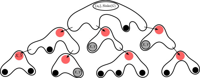
Figure 3: The figure shows the branching tree $\mathbb{T}_{\mathsf{br}}$ explored by our algorithm. The root is a call to $\mathsf{schedule}(\{s_{0}\},{{\textsf{sinks}}}(G))$. Black vertices are leaves of $\mathbb{T}_{\mathsf{br}}$, while red vertices are non-leaves corresponding to calls $\mathsf{schedule}(A,B)$ where $|B|\leq\left\lfloor\sqrt{nm}\right\rfloor$. We highlighted calls to $\mathsf{schedule}(X,Y)$ for some arbitrary $X,Y$. Using a lookup table, only one call to $(X,Y)$ is red and other calls to $(X,Y)$ are leaves. Decomposition $\mathcal{T}$ is created by deleting edges between red vertices and their parents.

Let $\lambda$ be a parameter (which we will set to $\lfloor\sqrt{nm}\rfloor$ to prove Theorem 1.1). Importantly, we highlight the non-leaf vertices of $\mathbb{T}_{\mathsf{br}}$ that correspond to calls $\mathsf{schedule}(A,B)$ for some $A$ and $B$ with $|B|\leq\lambda$, and color them in red (as shown in Fig. 3). We define $\mathcal{T}\coloneqq\{\tau_{1},\ldots,\tau_{k}\}$ to be the set of subtrees that arise from deleting all edges between red vertices and their parent in $\mathbb{T}_{\mathsf{br}}$ (except for the root of $\mathbb{T}_{\mathsf{br}}$ itself, which does not have a parent). Let $\tau_{\text{root}}\in\mathcal{T}$ be the tree that shares the same root as $\mathbb{T}_{\mathsf{br}}$. Our first goal is to bound the number of trees in $\mathcal{T}$.

Claim 4.2.

$|\mathcal{T}|\leq\binom{n}{\leq(m+\lambda)}+1$.

Proof. Every tree in $\mathcal{T}\setminus\{\tau_{\text{root}}\}$ has a root that is a red non-leaf vertex, and for each pair of sets $A,B$ with $|A|\leq m$ and $|B|\leq\lambda$ there is at most one non-leaf corresponding to the recursive call $\mathsf{schedule}(A,B)$. Moreover, the combination of jobs from $A$ and $B$ only appears once as $B\subseteq{{\textsf{succ}}}(A)$, so given a set $A\cup B$, one can determine $B$ by taking all jobs that have some predecessor in $A\cup B$. Hence, the total number of red non-leaves, and therefore the cardinality of $|\mathcal{T}|$, is at most $\binom{n}{\leq(m+\lambda)}+1$. $\blacksquare$

Now we bound the size of each tree in $\mathcal{T}$.

Claim 4.3.

$|\tau_{i}|\leq\binom{n}{\leq 2m}^{\left\lfloor n/\lambda\right\rfloor+1}$ for every $\tau_{i}\in\mathcal{T}$.

Proof. Observe that each vertex in $\tau_{i}$ has at most $\binom{n}{\leq 2m}$ children. This holds because in Line 1 of Algorithm 1, we iterate over two pairs of disjoint subsets $X$ and $Y$ of $\mathsf{Jobs}$ of size at most $m$ with $Y\subseteq{{\textsf{succ}}}(X)$. This is at most $\binom{n}{\leq 2m}$ because first, we can guess $X\cup Y$, and then the partition into $X$ and $Y$ is determined by the $Y\subseteq{{\textsf{succ}}}(X)$ relation.

Next, we show that the height (i.e., the number of edges on the longest path from the root to a leaf of the tree) of each tree $\tau_{i}$ is at most $\left\lfloor n/\lambda\right\rfloor+1$. By definition, tree $\tau_{i}$ does not have any red vertices except for its root. In other words, all vertices except the root represent calls $\mathsf{schedule}(A,B)$ for some $A$ and $|B|>\lambda$. According to 4.1, we have:

$$V(\mathrm{Int}(X,\mathsf{NewSinks}(X,Y)]) \subseteq V(\mathrm{Int}(A,B])\text{, and }$$

$$V(\mathrm{Int}(X,\mathsf{NewSinks}(X,Y)]) \cap B=\emptyset.$$

Note that by definition of the interval it holds that $B\subseteq V(\mathrm{Int}(A,B])$ because we assumed that $B\subseteq{{\textsf{succ}}}(A)$. Thus we have that $|V(\mathrm{Int}(X,\mathsf{NewSinks}(X,Y)])|\leq|V(\mathrm{Int}(A,B])|-|B|$ for every recursive call. In other words, in each recursive call the size of the instance decreases by at least $|B|$. Because initially $|V(\mathrm{Int}(A,B])|\leq n$ and $|B|>\lambda$ for each recursive call inside $\tau_{i}$ (except for the one that corresponds to the root of $\tau_{i}$), the total height of $\tau_{i}$ is thus at most $\left\lfloor n/\lambda\right\rfloor+1$. Combining the observations on the degree and height of $\tau_{i}$ proves the claim. $\blacksquare$

In total, the number of vertices in $\mathbb{T}_{\mathsf{br}}$ is at most $|\mathcal{T}|\cdot\max_{\tau_{i}\in\mathcal{T}}|\tau_{i}|$. Since one invocation of Lemma 3.6 takes $\binom{n}{\leq 2m}\cdot n^{\mathcal{O}(1)}$ time (see Lemma 3.6), each recursive call can be performed in $\binom{n}{\leq 2m}\cdot n^{\mathcal{O}(1)}$ time. Thus, we can conclude that Algorithm 1 has a running time of:

$$|\mathbb{T}_{\mathsf{br}}|\cdot\binom{n}{\leq 2m}\cdot n^{\mathcal{O}(1)}\leq\binom{n}{\leq(\lambda+m)}\binom{n}{\leq 2m}^{\left\lfloor n/\lambda\right\rfloor+2}\cdot n^{\mathcal{O}(1)}.$$ (1)

To obtain the running time from Theorem 1.1, we set $\lambda\coloneqq\left\lfloor\sqrt{nm}\right\rfloor$. Next, we use $\binom{n}{\leq(\lambda+m)}\leq\binom{n}{\leq\lambda}\cdot\binom{n}{\leq m}$ and the inequality $\binom{n}{\leq k}\leq(ne/k)^{k}$:

$$\left(\frac{ne}{\left\lfloor\sqrt{nm}\right\rfloor}\right)^{\left\lfloor\sqrt{nm}\right\rfloor}\cdot\left(\frac{ne}{m}\right)^{m}\cdot\left(\frac{ne}{2m}\right)^{\mathcal{O}(\sqrt{nm})}\cdot n^{\mathcal{O}(1)}=\left(1+\frac{n}{m}\right)^{\mathcal{O}(\sqrt{nm})}$$

as we can assume that $m\leq n$. This shows that Algorithm 1 runs in $\left(1+n/m\right)^{\mathcal{O}(\sqrt{nm})}$ time and establishes Theorem 1.1.

5 $\mathcal{O}(1.997^{n})$ Time Algorithm for Unbounded Number of Machines

In this section, we show how Theorem 1.1 can be used to obtain a significantly faster algorithm for $P\,|\,\mathrm{prec},p_{j}=1|\,C_{\max}$ , even when the number of machines is unbounded. To accomplish this, we first demonstrate in Subsection 5.1 how to obtain a fast algorithm when the number of machines is large. Next, in Subsection 5.2, we show how it can be utilized to prove Theorem 1.2.

5.1 An $\mathcal{O}^{\star}(2^{n-|{{\textsf{sinks}}}(G)|})$ Time Algorithm Using Fast Subset Convolution

Our algorithm crucially uses a technique that can be summarized in the following theorem:

Theorem 5.1 (Fast Subset Convolution [6]).

Given functions $f,g:2^{U}\rightarrow\{\mathsf{true,false}\}$. There is an algorithm that computes

$$(f\circledast g)(S)\coloneqq\bigvee_{Z\subseteq S}f(Z)\wedge g(S\setminus Z)$$

for every $S\subseteq U$ in $2^{|U|}\cdot|U|^{\mathcal{O}(1)}$ time.

Note that the above theorem is usually stated for functions $f,g$ with an arbitrary ring as co-domain, but is easy to see and well-known that the presented version also holds. We will use the algorithm implied by this theorem multiple times in our algorithm.

Lemma 5.2.

$P\,|\,\mathrm{prec},p_{j}=1|\,C_{\max}$ can be solved in $\mathcal{O}^{\star}(2^{n-|{{\textsf{sinks}}}(G)|})$ time.

Proof.

Let $G=(V,A)$ be the precedence graph given as input. We will compute the following functions: $f_{i,t},s_{i},a_{j}:2^{U}\rightarrow\{\mathsf{true,false}\}$ where $U\coloneqq V\setminus{{\textsf{sinks}}}(G)$. For any $X\subseteq V\setminus{{\textsf{sinks}}}(G)$, index $i\in\{0,1,\dots,n\}$ and $t\in\{0,\dots,n\}$ let

$$f_{i,t}(X) \coloneqq\begin{cases}\mathsf{true}&\text{if there exists a feasible schedule of makespan $t$ processing}\\ &\text{the jobs in $X$ jointly with $i$ jobs from ${{\textsf{sinks}}}(G)$, and $X={\textsf{pred}}[X]$,}\\ \mathsf{false}&\text{otherwise.}\end{cases}$$

Note that $$X={\textsf{pred}}[X] X\subseteq V\setminus{{\textsf{sinks}}}(G) i\in\{0,1,\dots,n\}$$ ensures that the schedule also includes all the predecessors of all the jobs. For any and define

$$s_{i}(X) \coloneqq\begin{cases}\mathsf{true}&\text{ if }|\{v\in{{\textsf{sinks}}}(G)\mid{\textsf{pred}}(v)\subseteq X\}|\geq i,\\ \mathsf{false}&\text{ otherwise.}\end{cases}$$

Intuitively, the value of $$s_{i}(X) X i Y\subseteq V\setminus{{\textsf{sinks}}}(G) j\in\{0,1,\dots,m\}$$ tells us whether the number of sinks that can be processed after processing is at least . For any and define

$$a_{j}(Y) \coloneqq\begin{cases}\mathsf{true}&\text{ if }|Y|\leq m-j\text{ and }Y\text{ is an antichain},\\ \mathsf{false}&\text{ otherwise.}\end{cases}$$

In essence, $a_{j}(Y)$ indicates whether $Y$ can be scheduled jointly with $j$ sinks that are not successors of $Y$ in a single timeslot.

It is important to note that the value $f_{|{{\textsf{sinks}}}(G)|,M}(V\setminus{{\textsf{sinks}}}(G))$ reveals whether all jobs can be completed within $M$ time units. Therefore, the smallest value of $M$ such that $f_{|{{\textsf{sinks}}}(G)|,M}(V\setminus{{\textsf{sinks}}}(G))=\mathsf{true}$ is the optimal makespan we search for.

We can efficiently determine the base-case $f_{i,0}(X)$ for all $X\subseteq V\setminus{{\textsf{sinks}}}(G)$ by setting $f_{i,0}(X)=\mathsf{true}$ if $X=\emptyset$ and $i=0$, and $f_{i,0}(X)=\mathsf{false}$ otherwise. For a fixed $Y\subseteq V\setminus{{\textsf{sinks}}}(G)$, $i\in\{0,\dots,n\}$, and $j\in\{0,1,\dots,m\}$, we can easily compute the values of $a_{j}(Y)$ and $s_{i}(Y)$ in polynomial time.

We calculate the values of $f_{i,t}(X)$ for every $t>0$, using the following recurrence relation.

Claim 5.3.

For all $X\subseteq V\setminus{{\textsf{sinks}}}(G)$, $i\in\{0,\dots,n\}$, $j\in\{0,\dots,m\}$ and $t\in\{1,\dots,n\}$:

$$f_{i,t}(X)=({X={\textsf{pred}}[X]})\wedge\left(\bigvee_{j\in\{0,\dots,m\}}\bigvee_{Y\subseteq X}f_{i-j,t-1}(X\setminus Y)\wedge s_{i}(X\setminus Y)\wedge a_{j}(Y)\right).$$ (2)

Proof. We split the claimed equivalence in two directions and prove them separately:

($\Rightarrow$): Assume that $f_{i,t}(X)=\mathsf{true}$. According to the definition, we have that $X={\textsf{pred}}[X]$ and there exists a feasible schedule $(T_{1},\dots,T_{t})$ that processes all jobs of $X$ and $i$ sinks. Select $Y=X\cap T_{t}$ as the set of jobs from $X$ that were processed at time $t$, and let $j=|T_{t}\cap{{\textsf{sinks}}}(G)|$ be the number of sinks processed at time $t$. We prove that this choice ensures that the right side of the equation is $\mathsf{true}$.

First, $f_{i-j,t-1}(X\setminus Y)$ is $\mathsf{true}$, since $(T_{1},\dots,T_{t-1})$ constitutes a feasible schedule for the jobs in $X\setminus Y$ and $i-j$ sinks. Second, $s_{i}(X\setminus Y)$ is $\mathsf{true}$, since all $i$ scheduled sinks (i.e., sinks in $\bigcup_{k=1}^{t}T_{k}$) must have all their predecessors in $X$, which were completed by the time $t-1$, implying that all predecessors of these jobs are in $X\setminus Y$. Additionally, $a_{j}(Y)$ is $\mathsf{true}$, as $j+|Y|\leq m$ and the jobs of $Y$ were all processed in the same timeslot of a feasible schedule, thereby meaning that $Y$ is an antichain.

($\Leftarrow$): If the right side of the equation is $\mathsf{true}$ it in particular means that there are $Y\subseteq X$, $j\in\{0,\dots,m\}$ such that $f_{i-j,t-1}(X\setminus Y)$, $s_{i}(X\setminus Y)$, and $a_{j}(Y)$ are all $\mathsf{true}$, and $X={\textsf{pred}}[X]$. Take $(T_{1},\dots,T_{t-1})$ as a feasible schedule for $X\setminus Y$ and $i-j$ sinks, which exists by definition of $f_{i-j,t-1}(X)$. Take $T_{t}=Y\cup B$, where $B$ is a subset of $\{v\in{{\textsf{sinks}}}(G)\mid{\textsf{pred}}(v)\subseteq X\setminus Y\}$ of size $j$ such that none of the jobs of $B$ are in $(T_{1},\dots,T_{t-1})$. Note that this set $B$ must exist as $s_{i}(X\setminus Y)$ is $\mathsf{true}$ and $(T_{1},\dots,T_{t-1})$ contains $i-j$ jobs of $\{v\in{{\textsf{sinks}}}(G)\mid{\textsf{pred}}(v)\subseteq X\setminus Y\}$.

We will prove that $(T_{1},\dots,T_{t-1},T_{t})$ is a feasible schedule for processing $X$ and $i$ sinks. Note that this schedule processes all of $X\setminus Y$ and $i-j$ sinks before time $t$, and $Y$ and $j$ sinks at time $t$. Thus, we need to show that this schedule is feasible, which means that no precedence constraints are violated. Since $(T_{1},\dots,T_{t-1})$ is feasible, we know that no precedence constraints within $X\setminus Y$ are violated and that the jobs in $B\cup Y$ cannot be predecessors of a job in $X\setminus Y$. Therefore, we only need to check whether $B\cup Y$ can start processing at time $t$. By definition of the jobs in $B$, we know that all of their predecessors are in $X\setminus Y$ and that these predecessors finish by time $t-1$, so no precedence constraints related to them are violated. Any predecessor of a job in $Y$ must be in $X\setminus Y$, because $X={\textsf{pred}}[X]$ and any predecessor must be in $X$, and since $Y$ is an antichain, it cannot be in $Y$. Therefore, we conclude that we have found a feasible schedule and that $f_{i,t}(X)$ is $\mathsf{true}$. $\blacksquare$

Now we show how to evaluate Eq. 2 quickly with Theorem 5.1. Instead of directly computing $f_{i,t}(X)$, we will compute two functions as intermediate steps. First, we compute for all $i\in\{0,\dots,n\}$, $j\in\{0,\dots,m\}$, $t\in\{0,\dots,n\}$, and $Z\subseteq U$:

$$p_{i,j,t}(Z) \coloneqq f_{i-j,t-1}(Z)\wedge s_{i}(Z).$$

Note that once the value of $$f_{i-j,t-1}(Z) p_{i,j,t}(Z) i\in\{0,\dots,n\} j\in\{0,\dots,m\} t\in\{0,\dots,n\} X\subseteq U$$ is known, the value of can be computed in polynomial time. Next, we compute for all , , and :

$$q_{i,j,t}(X) \coloneqq\bigvee_{Y\subseteq X}p_{i,j,t}(X\setminus Y)\wedge a_{j}(Y).$$

Once all values of $$p_{i,t-1}(X) q_{i,j,t}(X) X\subseteq U \mathcal{O}^{\star}(2^{n-|{{\textsf{sinks}}}(G)}|) X\subseteq U f_{i,t}(X) q_{i,j,t}(X)$$ are known, the values of for all can be computed in time using Theorem 5.1. Next, for every we determine the value of from as follows:

$$f_{i,t}(X) =(X={\textsf{pred}}[X])\wedge\bigvee_{j=0}^{m}q_{i,j,t}(X).$$

For every $X\subseteq V\setminus{{\textsf{sinks}}}(G)$, this transformation can be done in polynomial time. Therefore, all values of $f_{i,t}$ can be computed in $2^{n-|{{\textsf{sinks}}}(G)|}\cdot n^{\mathcal{O}(1)}$ time, assuming all values of $f_{i^{\prime},t-1}$ for $i^{\prime}\in\{0,1,\ldots,n\}$ are given. It follows that the minimum makespan of a feasible schedule for $G$ can be computed in $2^{n-|{{\textsf{sinks}}}(G)|}\cdot n^{\mathcal{O}(1)}$ time. This concludes the proof of Lemma 5.2. ∎

5.2 Proof of Theorem 1.2

Now we combine the algorithm from the previous subsection with Theorem 1.1 to prove Theorem 1.2.

First, observe that if a precedence graph has at most $m$ sinks, then there exists an optimal schedule that processes these sinks at the last timeslot. Moreover, only sinks can be processed at the last timeslot. Therefore, in such instances, we can safely remove all sinks and lower the target makespan by $1$ to get an equivalent instance.

It follows that we can assume that the number of sinks is at least $m$, and hence the algorithm from Lemma 5.2 runs in $\mathcal{O}^{\star}(2^{n-m})$ time. Set $\alpha=(1-\log_{2}(1.9969))\leq 0.002238$. If $m\geq\alpha n$, the algorithm from Lemma 5.2 runs in $\mathcal{O}(1.997^{n})$ time. Therefore, from now on, we assume that $m<\alpha n$.

We set $\lambda=0.15n$. Recall, that the Theorem 1.1 runs in (see Eq. 1):

$$\binom{n}{\lambda+m}\binom{n}{2m}^{\left\lfloor n/\lambda\right\rfloor+2}\cdot n^{\mathcal{O}(1)}$$

because $\lambda+m\leq n/4$. Next, we use the inequality $\binom{n}{pn}\leq 2^{h(p)n}\cdot n^{\mathcal{O}(1)}$ that holds for every $p\in(0,1)$, where $h(p)\coloneqq-p\log_{2}(p)-(1-p)\log_{2}(1-p)$ is the binary entropy. Therefore the running time is

$$2^{h(\lambda/n+\alpha)n}\cdot 2^{(\left\lfloor n/\lambda\right\rfloor+2)\cdot h(2\alpha)n}\cdot n^{\mathcal{O}(1)}.$$

Now, we plug in the exact value for $\alpha$ and $\lambda$. This gives $h(2\alpha)\leq 0.042$, $h(\lambda/n+\alpha)\leq 0.616$ and $\left\lfloor n/\lambda\right\rfloor=6$. Therefore, the running time is $\mathcal{O}^{\star}(2^{0.952n})$. This is faster than the $\mathcal{O}(1.997^{n})$ algorithm that we get in the case when $m\leq\alpha n$. By and large, this yields an $\mathcal{O}(1.997^{n})$ time algorithm for $P\,|\,\mathrm{prec},p_{j}=1|\,C_{\max}$ and proves Theorem 1.2.

6 Conclusion and Further Research

In this paper, our main results presents that $Pm\,|\,\mathrm{prec},p_{j}=1|\,C_{\max}$ can be solved in $(1+n/m)^{\mathcal{O}(\sqrt{nm})}$ time.

We hope that our techniques have the potential to improve the running time even further. In particular, it would already be interesting to solve $P3\,|\,\mathrm{prec},p_{j}=1|\,C_{\max}$ in time $\mathcal{O}(2^{n^{0.499}})$. However, even when the precedence graph is a subgraph of some orientation of a grid, we do currently not know how to improve the $2^{\mathcal{O}(\sqrt{n}\log n)}$ time algorithm.

As mentioned in the introduction, there are some interesting similarities between the research line of approximation initiated by [37] and our work: In these algorithms, the length of the highest chain $h$ also plays a crucial role. However, while we would need to get $h$ down to $\mathcal{O}(\sqrt{n})$ in order to ensure that the $n^{\mathcal{O}(h)}$ time algorithm of Dolev and Warmuth [16] runs fast enough, from the approximation point of view $h\leq\varepsilon n$ is already sufficient for getting a $(1+\varepsilon)$-approximation in polynomial time. Compared with the version from [14], both approaches also use a decomposition of some (approximately) optimal solution that eases the use of divide and conquer. An intriguing difference, however, is that the approach from [14] only uses polynomial space, whereas the memorization part of our algorithm is crucial. It is an interesting question whether memorization along with some of our other methods can be used to get a PTAS for $P3\,|\,\mathrm{prec},p_{j}=1|\,C_{\max}$ .

Another remaining question is how to exclude $2^{o(n)}$ time algorithms for $P\,|\,\mathrm{prec},p_{j}=1|\,C_{\max}$ when $m=\Theta(n)$ assuming the Exponential Time Hypothesis. In Appendix A, we show a $2^{\Omega(n)}$ lower bound assuming the Densest $\kappa$-Subgraph Hypothesis from [26], and it seems plausible that a similar bound assuming the Exponential Time Hypothesis exists as well. Currently, the highest ETH lower bound for $P\,|\,\mathrm{prec},p_{j}=1|\,C_{\max}$ is $2^{\Omega(\sqrt{n\log n})}$ due to Jansen, Land, and Kaluza [32].

Appendix A Lower Bound

Lenstra and Rinnooy Kan [36] proved the $\mathsf{NP}$-hardness of $P\,|\,\mathrm{prec},p_{j}=1|\,C_{\max}$ by reducing from an instance of Clique with $n$ vertices to an instance of $P\,|\,\mathrm{prec},p_{j}=1|\,C_{\max}$ with $\mathcal{O}(n^{2})$ jobs. Upon close inspection, their reduction gives a $2^{\Omega(\sqrt{n})}$ lower bound (assuming the Exponential Time Hypothesis). Jansen, Land, and Kaluza [32] improved this to $2^{\Omega(\sqrt{n\log n})}$. To the best of our knowledge, this is currently the best lower bound based on the Exponential Time Hypothesis. They also showed that a $2^{o(n)}$ time algorithm for $P\,|\,\mathrm{prec},p_{j}=1|\,C_{\max}$ would imply a $2^{o(n)}$ time algorithm for the Biclique problem on graphs with $n$ vertices.

We modify the reduction from [36] and start from an instance of the Densest $\kappa$-Subgraph problem on sparse graphs. In the Densest $\kappa$-Subgraph problem (D$\kappa$S), we are given a graph $G=(V,E)$ and a positive integer $\kappa$. The goal is to select a subset $S\subseteq V$ of $\kappa$ vertices that induce as many edges as possible. We use $\mathrm{den}_{\kappa}(G)$ to denote $\max_{S\subseteq V,|S|=\kappa}|E(S)|$, i.e., the optimum of D$\kappa$S. Recently, Goel et al. [26] formulated the following hypothesis about the hardness of D$\kappa$S.

Hypothesis A.1 ([26]).

There exists $\delta>0$ and $\Delta\in\mathbb{N}$ such that the following holds. Given an instance $(G,\kappa,\ell)$ of D$\kappa$S, where each one of $N$ vertices of graph $G$ has degree at most $\Delta$, no $\mathcal{O}(2^{\delta N})$ time algorithm can decide if $\mathrm{den}_{\kappa}(G)\geq\ell$.

In fact Goel et al. [26] formulated a stronger hypothesis about a hardness of approximation of D$\kappa$S. A.1 is a special case of [26, Hypothesis 1] with $C=1$. Now we exclude $2^{o(n)}$ time algorithms for $P\,|\,\mathrm{prec},p_{j}=1|\,C_{\max}$ assuming A.1. To achieve this we modify the $\mathsf{NP}$-hardness reduction of [36].

Theorem A.2.

Assuming A.1, no algorithm can solve $P\,|\,\mathrm{prec},p_{j}=1|\,C_{\max}$ in $2^{o(n)}$ time, even on instances with optimal makespan $3$.

Proof.

We reduce from an instance $(G,\kappa,\ell)$ of D$\kappa$S, as described in A.1. We assume that the graph $G$ does not contain isolated vertices. Note that if any isolated vertex is part of the optimum solution to D$\kappa$S, then the instance is trivial. We are promised that $G$ is an $N$-vertex graph with at most $M\leq\Delta N$ edges, for some constant $\Delta\in\mathbb{N}$.

Based on $(G,\kappa,\ell)$, we construct an instance of $P\,|\,\mathrm{prec},p_{j}=1|\,C_{\max}$ as follows. For each vertex $v\in V(G)$, create job $j_{v}^{(1)}$. For each edge $e=(u,v)\in E(G)$, create job $j_{e}^{(2)}$ with precedence constraints $j_{u}^{(1)}\prec j_{e}^{(2)}$ and $j_{v}^{(1)}\prec j_{e}^{(2)}$. Then, we set the number of machines $m\coloneqq 2\Delta N+1$ and create placeholder jobs. Specifically, we create three layers of jobs: Layer $L_{1}$ consists of $m-\kappa$ jobs, layer $L_{2}$ consists of $m+\kappa-\ell-N$ jobs, and layer $L_{3}$ consists of $m+\ell-M$ jobs. Finally, we set all the jobs in $L_{1}$ to be predecessors of every job in $L_{2}$, and all jobs in $L_{2}$ to be predecessors of every job in $L_{3}$. This concludes the construction of the instance. At the end, we invoke an oracle for $P\,|\,\mathrm{prec},p_{j}=1|\,C_{\max}$ and declare that $\mathrm{den}_{\kappa}(G)\geq\ell$ if the makespan of the schedule is $3$.

Now we argue that the constructed instance of $P\,|\,\mathrm{prec},p_{j}=1|\,C_{\max}$ is equivalent to the original instance of D$\kappa$S.

($\Rightarrow$): Assume that an answer to D$\kappa$S is true and there exists a set $S\subseteq V$ of $\kappa$ vertices that induce $\geq\ell$ edges. Then we can construct a schedule of makespan $3$ as follows. In the first timeslot, take jobs $j^{(1)}_{v}$ for all $v\in S$ and all jobs from layer $L_{1}$. In the second timeslot, take (i) jobs $j^{(1)}_{u}$ for all $v\in V\setminus S$, (ii) an arbitrary set of $\ell$ jobs $j^{(2)}_{e}$ where $e=(u,v)$ and $u,v\in S$, and (iii) all the jobs from $L_{2}$. In the third timeslot, take all the remaining jobs. Note that all precedence constraints are satisfied, and the sizes of $L_{1},L_{2}$, and $L_{3}$ are selected such that all timeslots fit $\leq m$ jobs.

($\Leftarrow$): Assume that there exists a schedule with makespan $3$. Since the total number of jobs $n$ is $3m$, every timeslot must be full, i.e., exactly $m$ jobs are scheduled in every timeslot. Observe that jobs from layers $L_{1},L_{2}$, and $L_{3}$ must be processed consecutively in timeslots $1$, $2$, and $3$ because every triple in $L_{1}\times L_{2}\times L_{3}$ forms a chain with $3$ vertices. Next, let $S\subseteq V$ be the set of vertices such that jobs $j^{(1)}_{s}$ with $s\in S$ are processed in the first timeslot. Note that, other than jobs from $L_{1}$, only $\kappa$ jobs of the form $j^{(1)}_{v}$ for some $v\in V$ can be processed in the first timeslot (as these are the only remaining sources in the graph). Now, consider a second timeslot, which must be filled by exactly $m$ jobs. There are exactly $N-\kappa$ jobs of the form $j^{(1)}_{v}$ for $v\in V\setminus S$, and exactly $m-\ell-(N-\kappa)$ jobs in $L_{2}$. Therefore, $\ell$ jobs of the form $j^{(2)}_{e}$ for some $e\in E(G)$ must be scheduled in the second timeslot. These jobs correspond to the edges of $G$ with both endpoints in $S$. Hence, $\mathrm{den}_{\kappa}(G)\geq\ell$.

This concludes the proof of equivalence between the instances. For the running time, note that the number of jobs $n$ in the constructed instance is $3m$, which is $\mathcal{O}(N)$ because $\Delta$ is a constant. Therefore, any algorithm that runs in $2^{o(n)}$ time and solves $P\,|\,\mathrm{prec},p_{j}=1|\,C_{\max}$ contradicts A.1. ∎

References

- [1] Noga Alon, Daniel Lokshtanov, and Saket Saurabh. Fast FAST. In Automata, Languages and Programming, 36th International Colloquium, ICALP 2009, volume 5555, pages 49–58. Springer, 2009.
- [2] László Babai. Graph isomorphism in quasipolynomial time [extended abstract]. In Proceedings of the 48th Annual ACM SIGACT Symposium on Theory of Computing, STOC 2016, pages 684–697. ACM, 2016.
- [3] Gábor Bacsó, Daniel Lokshtanov, Dániel Marx, Marcin Pilipczuk, Zsolt Tuza, and Erik Jan van Leeuwen. Subexponential-time algorithms for maximum independent set in -free and broom-free graphs. Algorithmica, 81(2):421–438, 2019.
- [4] Nikhil Bansal. Scheduling open problems: Old and new. MAPSP 2017, 2017.
- [5] Andreas Björklund. Determinant sums for undirected hamiltonicity. SIAM Journal on Computing, 43(1):280–299, 2014.
- [6] Andreas Björklund, Thore Husfeldt, Petteri Kaski, and Mikko Koivisto. Fourier meets Möbius: fast subset convolution. In Proceedings of the thirty-ninth annual ACM symposium on Theory of computing, pages 67–74. ACM, 2007.
- [7] Henrik Björklund, Sven Sandberg, and Sergei Vorobyov. A Discrete Subexponential Algorithm for Parity Games. In STACS 2003, pages 663–674. Springer Berlin Heidelberg, 2003.
- [8] Hans L. Bodlaender and Michael R. Fellows. [2]-hardness of precedence constrained -processor scheduling. Operations Research Letters, 18(2):93–97, 1995.
- [9] Hans L. Bodlaender, Carla Groenland, Jesper Nederlof, and Céline M.F. Swennenhuis. Parameterized Problems Complete for Nondeterministic FPT time and Logarithmic Space. In 62nd IEEE Annual Symposium on Foundations of Computer Science, FOCS 2021, pages 193–204, 2021.
- [10] Cristian S. Calude, Sanjay Jain, Bakhadyr Khoussainov, Wei Li, and Frank Stephan. Deciding parity games in quasi-polynomial time. SIAM J. Comput., 51(2):17–152, 2022.
- [11] Lin Chen, Klaus Jansen, and Guochuan Zhang. On the optimality of exact and approximation algorithms for scheduling problems. J. Comput. Syst. Sci., 96:1–32, 2018.
- [12] Edward G. Coffman and Ronald L. Graham. Optimal scheduling for two-processor systems. Acta informatica, 1(3):200–213, 1972.
- [13] Marek Cygan, Marcin Pilipczuk, Michał Pilipczuk, and Jakub Onufry Wojtaszczyk. Scheduling partially ordered jobs faster than . Algorithmica, 68(3):692–714, 2014.
- [14] Syamantak Das and Andreas Wiese. A Simpler QPTAS for Scheduling Jobs with Precedence Constraints. In 30th Annual European Symposium on Algorithms, ESA 2022, volume 244 of LIPIcs, pages 40:1–40:11, 2022.
- [15] Mark de Berg, Hans L. Bodlaender, Sándor Kisfaludi-Bak, Dániel Marx, and Tom C. van der Zanden. A Framework for Exponential-Time-Hypothesis-Tight Algorithms and Lower Bounds in Geometric Intersection Graphs. SIAM J. Comput., 49(6):1291–1331, 2020.
- [16] Danny Dolev and Manfred K. Warmuth. Scheduling precedence graphs of bounded height. Journal of Algorithms, 5(1):48–59, 1984.
- [17] Fedor V. Fomin, Erik D. Demaine, Mohammad Taghi Hajiaghayi, and Dimitrios M. Thilikos. Bidimensionality. In Encyclopedia of Algorithms, pages 203–207. 2016.
- [18] Fedor V. Fomin and Yngve Villanger. Subexponential Parameterized Algorithm for Minimum Fill-In. SIAM J. Comput., 42(6):2197–2216, 2013.
- [19] M. Fujii, T. Kasami, and K. Ninomiya. Optimal sequencing of two equivalent processors. SIAM Journal on Applied Mathematics, 17(4):784–789, 1969.
- [20] Harold N. Gabow. An almost-linear algorithm for two-processor scheduling. J. Assoc. Comput. Mach., 29(3):766–780, 1982.
- [21] Harold N. Gabow and Robert E. Tarjan. A linear-time algorithm for a special case of disjoint set union. Journal of computer and system sciences, 30(2):209–221, 1985.
- [22] Michael R. Garey and David S. Johnson. Computers and Intractability: A Guide to the Theory of -Completeness. W. H. Freeman, 1979.
- [23] Michael R. Garey, David S. Johnson, Robert E. Tarjan, and Mihalis Yannakakis. Scheduling opposing forests. SIAM Journal on Algebraic Discrete Methods, 4(1):72–93, 1983.
- [24] Shashwat Garg. Quasi-PTAS for Scheduling with Precedences using LP Hierarchies. In 45th International Colloquium on Automata, Languages, and Programming (ICALP 2018). Schloss Dagstuhl-Leibniz-Zentrum für Informatik, 2018.
- [25] Peter Gartland and Daniel Lokshtanov. Independent Set on -Free Graphs in Quasi-Polynomial Time. In 61st IEEE Annual Symposium on Foundations of Computer Science, FOCS 2020, Durham, NC, USA, November 16-19, 2020, pages 613–624. IEEE, 2020.
- [26] Surbhi Goel, Adam Klivans, Pasin Manurangsi, and Daniel Reichman. Tight Hardness Results for Training Depth-2 ReLU Networks. In 12th Innovations in Theoretical Computer Science Conference (ITCS 2021), volume 185 of Leibniz International Proceedings in Informatics (LIPIcs), pages 22:1–22:14. Schloss Dagstuhl–Leibniz-Zentrum für Informatik, 2021.
- [27] Ronald L. Graham. Bounds for certain multiprocessing anomalies. The Bell System Technical Journal, 45(9):1563–1581, 1966.
- [28] Ronald L. Graham, Eugene L. Lawler, Jan Karel Lenstra, and Alexander H.G. Rinnooy Kan. Optimization and Approximation in Deterministic Sequencing and Scheduling: a Survey. Annals of Discrete Mathematics, 5(2):287–326, 1979.
- [29] Michael Held and Richard M. Karp. A Dynamic Programming Approach to Sequencing Problems. Journal of the Society for Industrial and Applied mathematics, 10(1):196–210, 1962.
- [30] Michael Held, Richard M. Karp, and Richard Shareshian. Assembly-Line Balancing-Dynamic Programming with Precedence Constraints. Operations Research, 11(3):442–459, 1963.
- [31] Te C. Hu. Parallel sequencing and assembly line problems. Operations research, 9(6):841–848, 1961.
- [32] Klaus Jansen, Felix Land, and Maren Kaluza. Precedence Scheduling with Unit Execution Time is Equivalent to Parametrized Biclique. In International Conference on Current Trends in Theory and Practice of Informatics, pages 329–343. Springer, 2016.
- [33] Marcin Jurdziński, Mike Paterson, and Uri Zwick. A Deterministic Subexponential Algorithm for Solving Parity Games. SIAM J. Comput., 38(4):1519–1532, 2008.
- [34] James E. Kelley Jr. and Morgan R. Walker. Critical-path planning and scheduling. In Papers presented at the December 1-3, 1959, eastern joint IRE-AIEE-ACM computer conference, pages 160–173, 1959.
- [35] Eugene L. Lawler, Jan Karel Lenstra, Alexander H.G. Rinnooy Kan, and David B. Shmoys. Sequencing and scheduling: Algorithms and complexity. Handbooks in operations research and management science, 4:445–522, 1993.
- [36] Jan Karel Lenstra and Alexander H.G. Rinnooy Kan. Complexity of scheduling under precedence constraints. Operations Research, 26(1):22–35, 1978.
- [37] Elaine Levey and Thomas Rothvoß. A -Approximation for Makespan Scheduling with Precedence Constraints Using LP Hierarchies. SIAM J. Comput., 50(3), 2021.
- [38] Shi Li. Towards PTAS for precedence constrained scheduling via combinatorial algorithms. In Proceedings of the 2021 ACM-SIAM Symposium on Discrete Algorithms (SODA), pages 2991–3010. SIAM, 2021.
- [39] Eugene M. Luks. Isomorphism of Graphs of Bounded Valence can be Tested in Polynomial Time. J. Comput. Syst. Sci., 25(1):42–65, 1982.
- [40] Matthias Mnich and René van Bevern. Parameterized complexity of machine scheduling: 15 open problems. Computers & Operations Research, 2018.
- [41] Jesper Nederlof, Jakub Pawlewicz, Céline M.F. Swennenhuis, and Karol Węgrzycki. A Faster Exponential Time Algorithm for Bin Packing With a Constant Number of Bins via Additive Combinatorics. In Proceedings of the 2021 ACM-SIAM Symposium on Discrete Algorithms (SODA), pages 1682–1701. SIAM, 2021.
- [42] Jesper Nederlof, Céline M. F. Swennenhuis, and Karol Wegrzycki. Makespan scheduling of unit jobs with precedence constraints in o(1.995) time. CoRR, abs/2208.02664, 2022.
- [43] Christos H. Papadimitriou and Mihalis Yannakakis. Scheduling interval-ordered tasks. SIAM Journal on Computing, 8(3):405–409, 1979.
- [44] Petra Schuurman and Gerhard J Woeginger. Polynomial time approximation algorithms for machine scheduling: Ten open problems. Journal of Scheduling, 2(5):203–213, 1999.
- [45] Ravi Sethi. Scheduling graphs on two processors. SIAM J. Comput., 5(1):73–82, 1976.
- [46] Ola Svensson. Conditional hardness of precedence constrained scheduling on identical machines. In Proceedings of the forty-second ACM symposium on Theory of computing, pages 745–754, 2010.
- [47] Vincent T’kindt, Federico Della Croce, and Mathieu Liedloff. Moderate exponential-time algorithms for scheduling problems. 4OR, 20(4):533–566, 2022.
- [48] Jeffrey D. Ullman. -complete scheduling problems. Journal of Computer and System sciences, 10(3):384–393, 1975.