Gamma-ray spectra of the Crab, Vela and Geminga pulsars
fitted with SED of the emission from their current sheet

We show that the spectral energy distribution (SED) of the tightly focused radiation generated by the superluminally moving current sheet in the magnetosphere of a non-aligned neutron star fits the gamma-ray spectra of the Crab, Vela and Geminga pulsars over the entire range of photon energies so far detected by Fermi-LAT, MAGIC and H.E.S.S. from them: over $10^{2}$ MeV to $20$ TeV. While emblematic of any emission that entails caustics, the SED introduced here radically differs from those of the disparate emission mechanisms currently invoked in the literature to fit the data in different sections of these spectra. We specify, moreover, the connection between the values of the fit parameters for the analysed spectra and the physical characteristics of the central neutron stars of the Crab, Vela and Geminga pulsars and their magnetospheres.

1 Introduction

It is now firmly established that the magnetosphere of a non-aligned neutron star contains a rigidly rotating current sheet outside its light cylinder (see the review article Philippov & Kramer 2022 and the references therein). That this current sheet moves faster than light in vacuum is not incompatible with the requirements of special relativity because its superluminally moving distribution pattern is created by the correlated motion of subluminally moving charged particles (Bolotovskii & Bykov, 1990). The field generated by a constituent volume element of this current sheet embraces a synergy between the superluminal version of the field of synchrotron radiation and the vacuum version of the field of Čerenkov radiation (Ardavan, 2023, Sect. 2): the waves emanating from it possess a two-sheeted cusped envelope that spirals outward around the light cylinder all the way into the far zone (Ardavan, 2023, Figs. 3a and 4).

Only a single wave front propagates past an observer outside the envelope at any given time. But an observer inside the envelope receives three intersecting wave fronts, emanating from three distinct retarded positions of the source element simultaneously (Ardavan, 2023, Figs. 3b and 4). On each sheet of the envelope, two of these wave fronts coalesce and interfere constructively to generate an infinitely large radiation field in the time domain (Ardavan, 2021, Sect. 3.4). On the cusp locus of the envelope, where all three of these wave fronts (together with the three corresponding images of the source element) coalesce, the resulting radiation field has even a higher-order singularity (Ardavan, 2023, Figs. 5 and 6). Divergence of the field of a source point on the envelope and its cusp, which stems from the relativistic restrictions inherent in electrodynamics, reflects the fact that no superluminal source can be point-like. Superposition of the contributions from the constituent volume elements of the current sheet results in a field that, while sharply peaked, is finite (Ardavan, 2021, Sect. 4).

The field of the entire volume of the source receives its main contributions from those volume elements that approach the observer along the radiation direction with the speed of light and zero acceleration at the retarded time (Ardavan, 2021, Sect. 4.2). Phases of the waves emitted by such volume elements of the source possess two nearby stationary points that draw closer to each other the farther the waves are from their source (Ardavan, 2023, Fig. 7) and eventually coalesce at infinity. As a result, the waves in question constitute progressively more focused pulses, which by virtue of having time-domain profiles whose peaks get narrower the farther they propagate away from their source, embody the high-frequency component of the radiation from the current sheet (Ardavan, 2021, Sect. 5). The lower-frequency emission in the radio loud gamma-ray pulsars arises from the isolated stationary points of the phases of these waves (Ardavan, 2021, Sect. 5.4).

A detailed analysis of the radiation that is generated by the superluminally moving current sheet in the magnetosphere of a non-aligned neutron star can be found in Ardavan (2021). A heuristic account of the mathematical results of that analysis in more transparent physical terms is presented in Ardavan (2022) and Ardavan (2023, Sect. 2).

We begin here by deriving the spectral energy distribution (SED) of the most tightly focused component of the radiation that is emitted by the magnetospheric current sheet (Sect. 2). We then specify the values of the free parameters in the derived expression for which this SED best fits the data on the observed gamma-ray spectra of the Crab, Vela and Geminga pulsars (Sect. 3). The specified values of the fit parameters will be used, in conjunction with the results of the analysis in Ardavan (2021), to determine certain attributes of the central neutron stars of these pulsars and their magnetospheres in Sect. 4. The radical departure of the single explanation given here for the entire breadths of the analysed spectra from those normally given in terms of disjointed sets of ad hoc spectral distribution functions (such as simple or broken power-law functions with exponential cutoffs; see, e.g. Zanin 2017) and disparate emission mechanisms (such as synchro-curvature processes, inverse Compton scattering, or magnetic reconnection; see, e.g. The H.E.S.S. Collaboration et al. 2023) is briefly discussed in the final section of the paper (Sect. 5).

2 SED of the caustics generated by the superluminally moving current sheet

The frequency spectrum of the radiation that is generated by the superluminally moving current sheet in the magnetosphere of a non-aligned neutron star was presented, in its general form, in Ardavan (2021, Sect. 5.3). Here we derive the SED of the most tightly-focused component of this radiation from the general expression given in Eq. (177) of that paper.

In a case where the magnitudes of the vectors denoted by $\boldsymbol{\cal P}_{l}$ and $\boldsymbol{\cal Q}_{l}$ in Eq. (177) of Ardavan (2021) are appreciably larger than those of their counterparts, ${\bar{\boldsymbol{\cal P}}}_{l}$ and ${\bar{\boldsymbol{\cal Q}}}_{l}$, and the dominant contribution towards the Poynting flux $S_{\nu}$ of the radiation at the observation point is made by the term corresponding to $l=2$, Eq. (177) of Ardavan (2021) can be written as

$$S_{\nu}=\kappa_{0}\,k^{-2/3}\left|\boldsymbol{\cal P}_{2}\,{\rm Ai}(-k^{2/3}\sigma_{21}^{2})-{\rm i}k^{-1/3}\boldsymbol{\cal Q}_{2}\,{\rm Ai}^{\prime}(-k^{2/3}\sigma_{21}^{2})\right|^{2},$$ (1)

where Ai and ${\rm Ai}^{\prime}$ are the Airy function and the derivative of the Airy function with respect to its argument, respectively, $k=2\pi\nu/\omega$ is the frequency $\nu$ of the radiation in units of the rotation frequency $\omega/2\pi$ of the central neutron star, and $\kappa_{0}$ and $\sigma_{21}$ are two positive scalars. In the high-frequency regime $k\gg 1$, the coefficients of the Airy functions in the above expression stand for the complex vectors $\boldsymbol{\cal P}_{2}=k^{-1/2}\boldsymbol{\cal P}_{2}^{(2)}$ and $\boldsymbol{\cal Q}_{2}=k^{-1/2}\boldsymbol{\cal Q}_{2}^{(2)}$ in which $\boldsymbol{\cal P}_{2}^{(2)}$ and $\boldsymbol{\cal Q}_{2}^{(2)}$ are defined by Eqs (138)-(146) of Ardavan (2021). The variable $\sigma_{21}$ has a vanishingly small value at those privileged colatitudes (relative to the star’s spin axis) where the high-frequency radiation is observable (Ardavan, 2021, Sect. 4.5). For the purposes of the analysis in this paper, we may therefore replace $\boldsymbol{\cal P}_{2}^{(2)}$ and $\boldsymbol{\cal Q}_{2}^{(2)}$ by their limiting values for $k\gg 1$ and $0\leq\sigma_{21}\ll 1$ and treat them as constant parameters.

Multiplying Eq. (1) by the radiation frequency $\nu=\omega k/2\pi$ and expressing $\boldsymbol{\cal P}_{2}$ and $\boldsymbol{\cal Q}_{2}$ in terms of $\boldsymbol{\cal P}_{2}^{(2)}$ and $\boldsymbol{\cal Q}_{2}^{(2)}$, we find that the SED of this emission is given by

$$\nu S_{\nu} = \frac{\omega\kappa_{0}}{2\pi}k^{-2/3}\left|\boldsymbol{\cal P}^{(2)}_{2}\,{\rm Ai}(-k^{2/3}\sigma_{21}^{2})\right.$$ (2)

$$\left.-{\rm i}k^{-1/3}\boldsymbol{\cal Q}^{(2)}_{2}\,{\rm Ai}^{\prime}(-k^{2/3}\sigma_{21}^{2})\right|^{2}.$$

Evaluation of the right-hand side of Eq. (2) results in

$$\nu S_{\nu} = \kappa_{1}\,k^{-2/3}\left[{\rm Ai}^{2}(-k^{2/3}\sigma_{21}^{2})+\zeta_{1}^{2}k^{-2/3}{{\rm Ai}^{\prime}}^{2}(-k^{2/3}\sigma_{21}^{2})\right.$$ (3)

$$\left.+2\zeta_{1}\cos\beta\,k^{-1/3}{\rm Ai}(-k^{2/3}\sigma_{21}^{2}){\rm Ai}^{\prime}(-k^{2/3}\sigma_{21}^{2})\right],$$

where

$$\kappa_{1}=\frac{\omega\kappa_{0}}{2\pi}\left|\boldsymbol{\cal P}^{(2)}_{2}\right|^{2},\,\,\,\zeta_{1}=\frac{\left|{\boldsymbol{\cal Q}^{(2)}_{2}}\right|}{\left|{\boldsymbol{\cal P}^{(2)}_{2}}\right|},\,\,\,\cos\beta=\frac{\Im\left(\boldsymbol{\cal Q}^{(2)}_{2}\cdot\boldsymbol{\cal P}^{(2)*}_{2}\right)}{\left|\boldsymbol{\cal Q}^{(2)}_{2}\right|\left|\boldsymbol{\cal P}^{(2)}_{2}\right|},$$ (4)

and $\Im{}$ and $*$ denote an imaginary part and the complex conjugate, respectively. The above spectrum is emblematic of any radiation that entails caustics (see Stamnes, 1986).

To take account of the fact that the parameter $\sigma_{21}$ assumes a non-zero range of values across the (non-zero) latitudinal width of the detected radiation beam (Ardavan, 2021, Sect. 4.5), we must integrate $\nu S_{\nu}$ with respect to $\sigma_{21}$ over a finite interval $\rho\sigma_{0}\leq\sigma_{21}\leq\sigma_{0}$ with $\sigma_{0}\ll 1$ and $0\leq\rho<1$. Performing the integration of the Airy functions in Eq. (3) with respect to $\sigma_{21}$ by means of Mathematica, we thus obtain

$${\cal S}_{\nu} = \nu\int_{\rho\sigma_{0}}^{\sigma_{0}}S_{\nu}\,{\rm d}\sigma_{21}$$ (5)

$$= \kappa\left[f_{1}(\chi,\rho)+\frac{\zeta^{2}}{4\sqrt{3}}f_{2}(\chi,\rho)-\frac{\zeta\cos\beta}{2\sqrt{3}}f_{3}(\chi,\rho)\right],$$

where

$$\kappa=\left(\frac{\sigma_{0}}{\sqrt{3\pi}}\right)^{3}\kappa_{1},\qquad\zeta=\sigma_{0}\zeta_{1},\qquad\chi=\frac{2}{3}{\sigma_{0}}^{3}k,$$ (6)

$$f_{1} = \bigg{[}3\Gamma\left(\frac{7}{6}\right)\eta\chi^{-2/3}{}_{2}F_{3}\left(\begin{matrix}1/6&1/6&{}\\ 1/3&2/3&7/6\end{matrix};-\eta^{6}\chi^{2}\right)$$

$$+\pi^{1/2}\eta^{3}{}_{2}F_{3}\left(\begin{matrix}1/2&1/2&{}\\ 2/3&4/3&3/2\end{matrix}\,;-\eta^{6}\chi^{2}\right)$$

$$+\frac{9}{20}\Gamma\left(\frac{5}{6}\right)\eta^{5}\chi^{2/3}{}_{2}F_{3}\left(\begin{matrix}5/6&5/6&{}\\ 4/3&5/3&11/6\end{matrix}\,;-\eta^{6}\chi^{2}\right)\bigg{]}_{\eta=\rho}^{\eta=1},$$

$$f_{2}=\eta\chi^{-4/3}\,{}_{24}G^{31}\left(-\eta^{2}\chi^{2/3},\frac{1}{3}\left|\,\begin{matrix}5/6&7/6&{}&{}\\ 0&2/3&4/3&-1/6\end{matrix}\right)\right.\bigg{|}_{\eta=\rho}^{\eta=1},$$ (8)

$$f_{3}=\eta\chi^{-1}\,{}_{24}G^{31}\left(-\eta^{2}\chi^{2/3},\frac{1}{3}\left|\,\begin{matrix}5/6&1/2&{}&{}\\ 0&1/3&2/3&-1/6\end{matrix}\right)\right.\bigg{|}_{\eta=\rho}^{\eta=1},$$ (9)

and ${}_{2}F_{3}$ and ${}_{24}G^{31}$ are respectively the generalised hypergeometric function (see Olver et al., 2010) and the generalised Meijer G-Function . The variable $\chi$ that appears in the above expressions is related to the frequency $\nu$ of the radiation via $\chi=4\pi{\sigma_{0}}^{3}\nu/(3\omega)$.

The scale and shape of the SED given in Eq. (5) depend on the five parameters $\kappa$, $\zeta$, $\beta$, $\sigma_{0}$ and $\rho$: parameters whose values are dictated by the characteristics of the magnetospheric current sheet (see Sect. 4). The parameters $\zeta$, $\beta$ and $\rho$ determine the shape of the energy distribution while the parameters $\kappa$ and $\sigma_{0}$ determine the position of this distribution along the energy-flux and photon-energy axes, respectively.

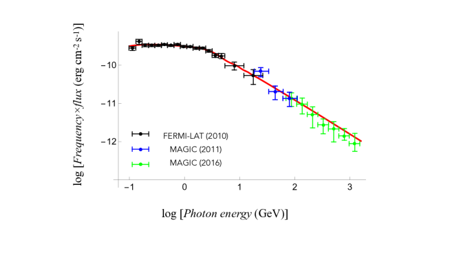
Figure 1: Phase-averaged gamma-ray spectrum of the Crab pulsar. The FERMI-LAT data points below $25$ GeV (coloured black) are those reported in Abdo et al. (2010). The MAGIC data points between $25$ and $100$ GeV (coloured blue) are those reported in Aleksić et al. (2011). The MAGIC data points beyond $100$ Gev (coloured green) are extracted, by the procedure described in Ardavan (2023, Sect. 4), from those reported by Ansoldi et al. (2016). The curve (coloured red) is a plot of the SED described by Eq. (5) for the parameters given in Eq. (10).

3 Fits to the gamma-ray data on the SEDs of the Crab, Vela and Geminga pulsars

In this section we use Mathematica’s ‘NonlinearModelFit’ procedure and the statistical information that it provides to determine the values of the fit parameters and their standard errors. Where, owing to the complexity of the expression in Eq. (5), this procedure breaks down and so the fits to the data are obtained by trial and error, only the values of these parameters are specified. The fit residuals in the case of each pulsar turn out to be smaller than the corresponding observational errors for almost all data points (see Figs. 1–3). Since there are no two values of any of the fit parameters for which the present SED has the same shape and position, the specified values of the fit parameters are moreover unique.

3.1 Spectrum of the Crab pulsar (PSR J0534+2200)

Figure 1 shows the data on the energy spectrum of the phase-averaged gamma-ray emission from the Crab pulsar (Abdo et al., 2010; Aleksić et al., 2011; Ansoldi et al., 2016) and a plot of the SED described by Eq. (5) that fits them best. The parameters for which the function ${\cal S}_{\nu}(\chi)$ (depicted by the red curve in this figure) is plotted have the following values and standard errors:

$$\kappa = (8.15\pm 0.75)\times 10^{-11}\quad{\rm erg}\,{\rm cm}^{-2}\,{\rm s}^{-1},$$

$$\chi = (0.576\pm 0.095)\times(h\nu)_{\rm GeV},$$

$$\sigma_{0} = (4.76\pm 2.61)\times 10^{-8},\,\,\,\zeta=0.394\pm 0.076,$$

$$\beta = 0.258\pm 0.249,\quad\rho=0,$$ (10)

where $h$ stands for the Planck constant and $2\pi/\omega$ has been set equal to the period of the Crab pulsar ($0.033$ s). Figure 1 was first reported in Ardavan (2023) but with an incorrect label on its vertical axis.

As the photon energy $h\nu$ increases beyond $1.2$ TeV, the slope of the curve in Fig. 1 continues to decrease at the relatively slow rate in which it decreases past $50$ GeV. Thus the upper limits given by Ansoldi et al. (2016) for the flux density of gamma-rays whose energies exceed $1.2$ TeV all lie above the continuation of the curve shown in Fig. 1.

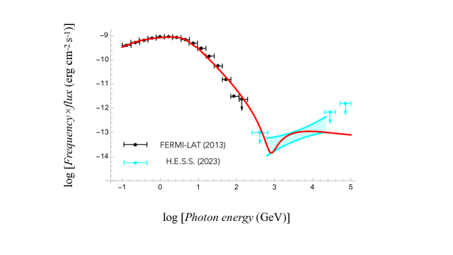
Figure 2: Gamma-ray spectrum of the Vela pulsar. The FERMI-LAT data points below $10^{2}$ GeV (coloured black) are those reported in Abdo et al. (2013). The H.E.S.S. data above $260$ GeV (shown as the magenta area between $1\sigma$ uncertainty bands and the magenta upper limits) are those reported in The H.E.S.S. Collaboration et al. (2023). The curve (coloured red) is a plot of the SED described by Eq. (5) for the parameters given in Eqs. (11) and (12).

3.2 Spectrum of the Vela pulsar (PSR J0835-4510)

The data on the Vela pulsar both in the GeV band detected by Fermi-LAT (Abdo et al., 2013) and in the TeV band detected by H.E.S.S. (The H.E.S.S. Collaboration et al., 2023) are shown in Fig. 2. The SED that best fits these data (represented by the red curve in Fig. 2) is described by the expression in Eq. (5) for the following values of its free parameters:

$$\kappa = (3.31\pm 0.047)\times 10^{-10}\quad{\rm erg}\,{\rm cm}^{-2}\,{\rm s}^{-1},$$

$$\chi = (0.436\pm 0.071)\times(h\nu)_{\rm GeV},$$

$$\sigma_{0} = (3.12\pm 1.70)\times 10^{-8},\quad\zeta=0.518\pm 0.065,$$

$$\beta = 0.244\pm 0.073,\quad\rho=0.409\pm 0.198,$$ (11)

over the range $0.1\leq(h\nu)_{\rm GeV}\leq 10$ and

$$\kappa = 7.94\times 10^{-13}\quad{\rm erg}\,{\rm cm}^{-2}\,{\rm s}^{-1},$$

$$\chi = 2.51\times 10^{-6}\times(h\nu)_{\rm GeV},$$

$$\sigma_{0} = 5.59\times 10^{-10},\,\,\zeta=0.203,\,\,\beta=0.105,\,\,\rho=0.99,$$ (12)

over the range $10\leq(h\nu)_{\rm GeV}\leq 2\times 10^{4}$ of photon energies.

The difference between the values of the free parameters in the above two ranges of photon energies stems from the fact that the higher-frequency radiation is appreciably more focused than its lower-frequency counterpart in this case. This is reflected not only in the much lower value of $\sigma_{0}$ in Eq. (12) compared to that in Eq. (11), but also in the higher value of $\rho$ (i.e. the shorter range of values of $\sigma_{21}$): the smaller the value of $\sigma_{21}$, the closer to each other are the stationary points of the phases of the emitted waves and so the more focused is the radiation (Ardavan, 2021, Sect. 4.5).

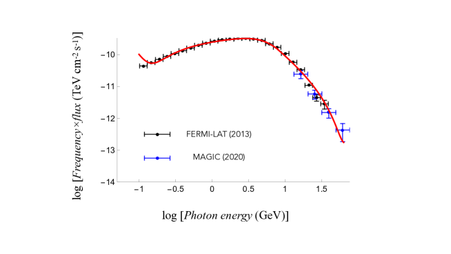
Figure 3: Gamma-ray spectrum of the Geminga pulsar. The FERMI-LAT data points below $35$ GeV (coloured black) are those reported in Abdo et al. (2013). The MAGIC data points above $35$ GeV (coloured blue) are those reported in The MAGIC Collaboration et al. (2020). The curve (coloured red) is a plot of the SED described by Eq. (5) for the parameters given in Eqs. (13) and (14).

3.3 Spectrum of the Geminga pulsar (PSR J0633+1746)

The Fermi-LAT (Abdo et al., 2013) and MAGIC (The MAGIC Collaboration et al., 2020) data on the gamma-ray emission from the Geminga pulsar are shown in Fig. 3. The fit to these data (the red curve in Fig 3) is described by the expression in Eq. (5) for

$$\kappa = (1.47\pm 0.23)\times 10^{-10}\quad{\rm TeV}\,{\rm cm}^{-2}\,{\rm s}^{-1},$$

$$\chi = (0.392\pm 0.038)\times(h\nu)_{\rm GeV},$$

$$\sigma_{0} = (2.17\pm 0.99)\times 10^{-8},\quad\zeta=0.646\pm 0.028$$

$$\beta = 0.194\pm 0.017,\quad\rho=0.568\pm 0.131,$$ (13)

over the range $0.1\leq(h\nu)_{\rm GeV}\leq 7.94$ and

$$\kappa = 1.01\times 10^{-13}\quad{\rm TeV}\,{\rm cm}^{-2}\,{\rm s}^{-1},$$

$$\chi = 3.98\times 10^{-6}\times(h\nu)_{\rm GeV},$$

$$\sigma_{0} = 4.71\times 10^{-10},\,\,\zeta=0.101,\,\,\beta=0.071,\,\,\rho=0.511,$$ (14)

over the range $7.94\leq(h\nu)_{\rm GeV}\leq 63.1$ of photon energies. As in the case of the spectrum of the Vela pulsar, the change in the values of the fit parameters across $(h\nu)_{\rm GeV}=7.94$ reflects the fact that the higher-frequency radiation is appreciably more focused than its lower-frequency counterpart.

4 The connection between the parameters of the fitted spectra and the physical characteristics of their sources

From Eqs. (6), (4) and (1), it follows that the parameters $\kappa$, $\zeta$, $\rho$ and $\sigma_{0}$ in Eq. (5) are related to the characteristics of the source of the observed radiation via the quantities $\omega$, $\kappa_{0}$, $\boldsymbol{\cal P}_{2}^{(2)}$ and $\boldsymbol{\cal Q}_{2}^{(2)}$ that appear in the expression for the SED ${\cal S}_{\nu}$. In this section we use the results of the analysis presented in Ardavan (2021) to express these quantities in terms of the inclination angle of the central neutron star, $\alpha$, the magnitude of the star’s magnetic field at its magnetic pole, $B_{0}=10^{12}{\hat{B}}_{0}$ Gauss, the radius of the star, $r_{s0}=10^{6}d$ cm, the rotation frequency of the star, $\omega=10^{2}{\hat{P}}^{-1}$ rad/s, and the spherical polar coordinates, $R_{P}=D\,\,{\rm kpc}=3.085\times 10^{21}D$ cm, $\varphi_{P}$ and $\theta_{P}$, of the observation point $P$ in a frame whose centre and $z$-axis coincide with the centre and spin axis of the star.

When $\sigma_{21}\ll 1$ and so the quantities $\tau_{2{\rm min}}$ and $\tau_{2{\rm max}}$ that appear in Eqs. (177), (138)–(146) and (136) of Ardavan (2021) are approximately equal, these equations imply that

$$\kappa_{0}=4.15\times 10^{18}w_{1}^{2}w_{3}^{2}{\hat{B}}_{0}^{2}d^{4}D^{-2}{\hat{P}}^{-1}\quad{\rm Jy},$$ (15)

and

$$\left|\boldsymbol{\cal P}_{2}^{(2)}\right|=\frac{b}{3}\left(\frac{2}{\pi a^{3}}\right)^{1/2}\left(\frac{2\sigma_{21}}{\partial^{2}f_{2C}/\partial\tau^{2}|_{\tau=\tau_{2{\rm min}}}}\right)^{1/2}\left|{\tilde{\bf P}}_{2}\right|,$$ (16)

where

$$w_{1}=\left|1-2\alpha/\pi\right|,\qquad w_{3}=1+0.2\sin^{2}\alpha,$$ (17)

$$f_{2C} = ({\hat{r}}_{P}^{2}{\hat{r}}_{sC}^{2}\sin^{2}\theta-1)^{1/2}-{\hat{R}}_{P}-\arccos\left({\hat{r}}_{P}^{-1}{\hat{r}}_{sC}^{-1}\csc\theta\right)$$ (18)

$$-\arccos(\cot\alpha\cot\theta)+{\hat{r}}_{sC}+\varphi_{P}-{\hat{r}}_{s0}-2\pi,$$

$$a = ({\hat{r}}_{P}^{2}{\hat{r}}_{sC}^{2}\sin^{2}\theta-1)\left[\frac{({\hat{r}}_{P}^{2}{\hat{r}}_{sC}^{2}\sin^{2}\theta-1)^{1/2}+{\hat{r}}_{sC}}{{\hat{r}}_{sC}({\hat{r}}_{P}^{2}-1)^{1/2}({\hat{R}}_{P}^{2}\sin^{2}\theta-1)^{1/2}}\right.$$ (19)

$$\left.-\frac{1}{({\hat{r}}_{P}^{2}{\hat{r}}_{sC}^{2}\sin^{2}\theta-1)^{1/2}}\right],$$

$$b=\frac{{\hat{r}}_{P}^{2}{\hat{r}}_{sC}^{2}\sin^{2}\theta-1}{{\hat{r}}_{sC}({\hat{r}}_{P}^{2}-1)^{1/2}({\hat{R}}_{P}^{2}\sin^{2}\theta-1)^{1/2}},$$ (20)

$${\hat{r}}_{sC}=\frac{({\hat{r}}_{P}^{2}-1)^{1/2}({\hat{R}}_{P}^{2}\sin^{2}\theta-1)^{1/2}-{\hat{z}}_{P}\cos\theta}{{\hat{r}}_{P}^{2}\sin^{2}\theta-1},$$ (21)

$$\sigma_{21}=[{\textstyle\frac{3}{4}}(f_{2C}|_{\tau=\tau_{2{\rm max}}}-f_{2C}|_{\tau=\tau_{2{\rm min}}})]^{1/3},$$ (22)

$$\theta=\arccos(\sin\alpha\cos\tau),$$ (23)

$$\left|{\tilde{\bf P}}_{2}\right| = \cos\alpha[{\hat{r}}_{sC}^{2}(1+\cos^{2}\theta_{P}-2\cos\theta\cos\theta_{P})+\tan^{2}\alpha$$

$$-\cot^{2}\theta+2{\hat{r}}_{sC}\sin\theta\cos\theta_{P}(\tan^{2}\alpha-\cot^{2}\theta)^{1/2}]^{1/2},\quad\,\,$$

and the variables $\tau_{2{\rm min}}$ and $\tau_{2{\rm max}}$ stand for the minimum and maximum of the function $f_{2C}$ (see also Eqs. (7), (9), (174), (175), (93)–(95), (97) and (88) of Ardavan 2021). The caret on $R_{P}$ and $r_{s0}$ (and $r_{P}=R_{P}\sin\theta_{P}$, $z_{P}=R_{P}\cos\theta_{P}$) is used here to designate a variable that is rendered dimensionless by being measured in units of the light-cylinder radius $c/\omega$. (Note the following two corrections: the vector ${\bf P}_{2}$ in Eq. (145) and the numerical coefficient $1.54\times 10^{19}$ in Eq. (177) of Ardavan 2021 have been corrected to read ${\tilde{\bf P}}_{2}$ and $4.15\times 10^{18}$, respectively.)

The expression for $|{\tilde{\bf P}}_{2}|$ in Eq. (LABEL:E24) is derived from that for ${\bf P}_{2}$ given by Eqs. (98), (80), (78) and (62) of Ardavan (2021). In this derivation, we have set the observation point on the cusp locus of the bifurcation surface where ${\hat{r}}_{s}={\hat{r}}_{sC}$, have approximated $(p_{1},p_{2},p_{3})$ by its far-field value $2^{1/3}{\hat{R}}_{P}^{-1}({\hat{R}}_{P}^{-1},-1,1)$ and have let ${\bf P}_{2}={\hat{R}}_{P}^{-1}{\tilde{\bf P}}_{2}$. The factor ${\hat{R}}_{P}^{-2}$ that would have otherwise appeared in the resulting expression for $|\boldsymbol{\cal P}^{(2)}_{2}|^{2}$ is thus incorporated in the factor $\kappa_{0}$ in Eq. (15).

For certain values of $\theta_{P}$, denoted by $\theta_{P2S}$, the function $f_{2C}(\tau)$ has an inflection point (see Ardavan 2021, Sect. 4.4, and Ardavan 2023, Sect. 2). For any given inclination angle $\alpha$, the position $\tau_{2S}$ of this inflection point and the colatitude $\theta_{P2S}$ of the observation points for which $f_{2C}(\tau)$ has an inflection point follow from the solutions to the simultaneous equations $\partial f_{2C}/\partial\tau=0$ and $\partial^{2}f_{2C}/\partial\tau^{2}=0$. (Explicit expressions for the derivatives that appear in these equations can be found in Appendix A of Ardavan 2021.) For values of $\theta_{P}$ close to $\theta_{P2S}$, the separation between the maximum $\tau=\tau_{2{\rm max}}$ and minimum $\tau=\tau_{2{\rm min}}$ of $f_{2C}$ and hence the value of $\sigma_{21}$ are vanishingly small. Since the high-frequency radiation that arises from the current sheet is detectable only in the vicinity of the latitudinal direction $\theta_{P}=\theta_{P2S}$ (see Fig. 4), here we have evaluated the variables that appear in Eqs. (16)–(LABEL:E24) for $\sigma_{21}\ll 1$. The ratio appearing inside the second pair of parentheses in Eq. (16), which becomes indeterminate as $\sigma_{21}$ tends to zero, approaches a finite value in this limit.

The dimensionless frequency $k=2\pi\nu/\omega$ of a $1$ GeV photon has the value $8\times 10^{21}$ in the case of the Crab pulsar. In contrast, as indicated by the small values of the fit parameter $\sigma_{0}$ encountered in Sect. 3, the value of the variable $\chi=2\sigma_{0}^{3}k/3$ that appears in the description of the SED ${\cal S}_{\nu}$ is of the order of $10^{-3}$ for a $1$ GeV gamma-ray photon. Because any measurement of the spectrum described by Eq. (5) is carried out by counting the number of detected gamma-ray photons in a bin covering an energy interval of a few MeV or GeV, the widths of the equivalent frequency bins involved in such measurements are of the order of $\Delta k=3\sigma_{0}^{-3}\Delta\chi/2$ with $10^{-4}\lesssim\Delta\chi\lesssim 10^{-2}$.

Once the the expression for the SED ${\cal S}_{\nu}$ is accordingly multiplied by $3\sigma_{0}^{-3}\Delta\chi/2$, Eqs. (6), (4), (15) and (16) jointly yield

$$\kappa=2.42\times 10^{-6}{\hat{B}}_{0}^{2}d^{4}D^{-2}{\hat{P}}^{-2}\Delta\chi\,{\hat{\kappa}}_{\rm th}\qquad{\rm erg}\,\,{\rm s}^{-1}{\rm cm}^{-2},$$ (25)

in which

$${\hat{\kappa}}_{\rm th}=w_{1}^{2}w_{3}^{2}\frac{b^{2}}{a^{3}}\left(\frac{2\sigma_{21}}{\partial^{2}f_{2C}/\partial\tau^{2}|_{\tau=\tau_{2{\rm min}}}}\right)\left|{\tilde{\bf P}}_{2}\right|^{2},$$ (26)

and Jy has been expressed in terms of erg s^-1 cm^-2 Hz^-1. Equation (25) can be written as ${\hat{\kappa}}_{\rm th}={\hat{\kappa}}_{\rm obs}$, where

$${\hat{\kappa}}_{\rm obs}=4.13\times 10^{5}({\hat{B}}_{0}d^{2})^{-2}(\Delta\chi)^{-1}D^{2}{\hat{P}}^{2}\kappa.$$ (27)

While ${\hat{\kappa}}_{\rm obs}$ only contains the observed parameters of the pulsar and its emission, the value of ${\hat{\kappa}}_{\rm th}$ is determined by the physical characteristics of the magnetospheric current sheet that acts as the source of the observed emission. When, as in Fig. 20 of Ardavan (2021), the value of the colatitude $\theta_{P}$ of the observation point is sufficiently close to that of the critical angle $\theta_{P2S}$ for $|\tau_{2{\rm max}}-\tau_{2{\rm min}}|$ and hence $\sigma_{21}$ to be much smaller than unity, the right-hand side of Eq. (26) is a function of the inclination angle $\alpha$ and the observer’s distance ${\hat{R}}_{P}$ only.

Equation (25) thus enables us to connect the the parameters of the fitted spectra to the physical characteristics of their sources.

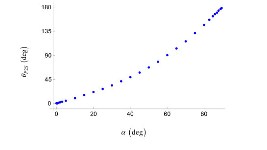
Figure 4: The dependence on the star’s inclination angle $\alpha$ of the critical colatitude $\theta_{P2S}$ along which the high-frequency radiation beam generated by the superluminally moving current sheet propagates.

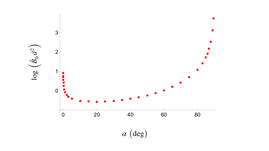
Figure 5: Dependence of the ${\hat{B}}_{0}d^{2}$ on $\alpha$ for the Crab pulsar, where ${\hat{B}}_{0}$ is the magnitude of the star’s magnetic field at its magnetic pole in units of $10^{12}$ Gauss, $d$ is the radius of the star in units of $10^{6}$ cm and $\alpha$ is the angle between the magnetic and rotation axes of the star in degrees.

4.1 Characteristics of the source of the Crab pulsar’s emission

Once the value of the fit parameter $\kappa$ given in Eq. (10), the period ($0.033$ s) and the distance ($2$ kpc) of the Crab pulsar are inserted in Eq. (27), the resulting value of ${\hat{\kappa}}_{\rm obs}$ can be equated to ${\hat{\kappa}}_{\rm th}$ to obtain

$${\hat{B}}_{0}d^{2}=1.93\times 10^{-1}{\hat{\kappa}}_{\rm th}^{-1/2}$$ (28)

for $\Delta\chi=10^{-3}$. The dependence of ${\hat{B}}_{0}d^{2}$ on $\alpha$ implied by this relationship, in conjunction with Eq. (26), is plotted in Fig. 5.

One can infer from the separation between the two peaks in the gamma-ray light curve of the Crab pulsar  ($\sim 0.4$ cycles; Abdo et al., 2010) that the inclination angle $\alpha$ of this pulsar has a value lying in the range $60^{\circ}$ to $70^{\circ}$ (Ardavan, 2021, Sect. 5.4). This in turn implies that the value of ${\hat{B}}_{0}d^{2}$ lies between $1.05$ and $2.61$ in this case (see Fig. 5), i.e. that the magnitude of the star’s magnetic field at its magnetic pole lies in the range $1.05\times 10^{12}$ to $2.61\times 10^{12}$ Gauss if we assume that the star’s radius has the value $10^{6}$ cm. These are of the same order of magnitude as the value of $B_{0}$ obtained from the conventional formula for magnetic dipole radiation (i.e. $3.79\times 10^{12}$ Gauss; Manchester et al. 2005).

The corresponding value of the privileged latitudinal direction $\theta_{P2S}$ in which the high-frequency radiation from the Crab pulsar can be observed lies between $90^{\circ}$ and $117^{\circ}$ according to Fig. 4. The range of values of the inclination angle $\alpha$ determines also the scale factor $j_{0}$ of the electric current density in the magnetosphere of the pulsar: from Eq. (22) of Ardavan (2021) it follows that

$$j_{0}=1.29\times 10^{8}{\hat{B}}_{0}d^{2}{\hat{P}}^{-3}w_{1}w_{3},\qquad{\rm statamp\,cm}^{-2}$$ (29)

a scale factor whose value lies between $3.55\times 10^{8}$ and $6.01\times 10^{8}$ statamp cm^-2 in the case of the Crab pulsar.

The above results supersede those reported in Ardavan (2023, Sect. 4).

4.2 Characteristics of the source of the Vela pulsar’s emission

Properties of the central neutron star of the Vela pulsar and its magnetosphere are more accurately reflected in the parameters of its spectrum over the photon energies $0.1$ to $10$ GeV, i.e. the interval that encompasses the majority of the data points plotted in Fig. 2. Insertion of the value of the fit parameter $\kappa$ given in Eq. (11), the period ($0.089$ s) and the distance ($287$ pc) of this pulsar in Eq. (27), together with ${\hat{\kappa}}_{\rm obs}={\hat{\kappa}}_{\rm th}$, results in

$${\hat{B}}_{0}d^{2}=1.50\times 10^{-1}{\hat{\kappa}}_{\rm th}^{-1/2}$$ (30)

for $\Delta\chi=10^{-3}$. Thus the dependence of ${\hat{B}}_{0}d^{2}$ on $\alpha$ is given by a shifted version of the curve in Fig. 5: one that is vertically lowered by 0.109 (cf. Eqs. (28) and (30)).

If we assume that the radius of the central neutron star of this pulsar has the value $10^{6}$ cm, i.e. $d=1$, then the value $3.38\times 10^{12}$ Gauss of its magnetic field $B_{0}$ (inferred from the conventional formula for magnetic dipole radiation; Manchester et al. 2005) corresponds, according to the modified version of Fig. 5, to the inclination angle $\alpha=70^{\circ}$. This would in turn imply, in conjunction with Eq. (29) and Fig. 4, that the scale factor $j_{0}$ of the electric current density has the value $4.02\times 10^{7}$ statamp cm^-2 and the latitudinal direction along which the pulsar is observed is given by $\theta_{P2S}=117^{\circ}$.

That the main peaks of the gamma-ray light curve of the Vela pulsar are separated by $\sim 0.43$ cycles (The H.E.S.S. Collaboration et al., 2023) is consistent with an inclination angle close to $70^{\circ}$ (see Ardavan, 2021, Sect. 5.4).

4.3 Characteristics of the source of the Geminga pulsar’s emission

The value of $\kappa$ given in Eq. (13), which applies to a wider range of photon energies than that given in Eq. (14), together with the period ($0.237$ s) and the distance ($190$ pc) of the Geminga pulsar yield

$${\hat{B}}_{0}d^{2}=2.24\times 10^{-1}{\hat{\kappa}}_{\rm th}^{-1/2}$$ (31)

for $\Delta\chi=10^{-3}$ (see Eq. (27) and recall that ${\hat{\kappa}}_{\rm obs}={\hat{\kappa}}_{\rm th}$). The dependence of ${\hat{B}}_{0}d^{2}$ on $\alpha$ is therefore given by a set of points whose only difference with those plotted in Fig. 5 is that their vertical coordinates are shifted upward by $0.065$ (cf. Eqs. (28) and (31)).

Given that the two peaks of the gamma-ray light curve of this pulsar are separated by $\sim 0.5$ cycle (The MAGIC Collaboration et al., 2020), the inclination angle of its central neutron star must be about $60^{\circ}$ (Ardavan, 2021, Sect. 5.4). This, together with the modified version of Fig. 5, implies the value ${\hat{B}}_{0}\simeq 1.22$, i.e. $B_{0}=1.22\times 10^{12}$ Gauss, for the magnetic field of the star at its pole (when $d=1$), a value that is not too different from that predicted by the conventional expression for magnetic dipole radiation, i.e. $1.63\times 10^{12}$ Gauss (Manchester et al., 2005). Equation (29) and Fig. 4 respectively yield $j_{0}=1.12\times 10^{6}$ statamp cm^-2 and $\theta_{P2S}=90^{\circ}$ for the scale factor of the electric current density and the colatitude of the observation point in this case.

5 Concluding remarks

An up to date discussion of the emission mechanisms that have so far been proposed for explaining the data on the observed gamma-ray spectra of pulsars can be found in The H.E.S.S. Collaboration et al. (2023). Even in the most favourable circumstances, spectra of the emissions from relativistic charged particles that are accelerated by synchro-curvature, inverse Compton or magnetic reconnection processes fit the observed data only over disjoint limited ranges of photon energies. In particular, the constraints set by the $20$ TeV component of the radiation from the Vela pulsar “provide unprecedented challenges to the state-of-the-art models of HE [high energy] and VHE [very high energy] emission from pulsars” (The H.E.S.S. Collaboration et al., 2023).

In contrast, the SED of the tightly focused caustics that are generated by the superluminally moving current sheet in the magnetosphere of a non-aligned neutron star fits the observed spectra of the Crab, Vela and Geminga pulsars over the entire range of photon energies so far detected by Fermi-LAT, MAGIC and H.E.S.S. from them: over $10^{2}$ MeV to $20$ TeV. Not only are these data fitted by a single spectral distribution function but they are also explained by a single emission mechanism, an emission mechanism that has already accounted for a number of other salient features of the radiation received from pulsars: its brightness temperature, polarization, radio spectrum, and profile with microstructure and with a phase lag between the radio and gamma-ray peaks (Ardavan, 2021, 2022).

Two final remarks concerning the analysis that has led to the present SED are in order:

(i)

It is often presumed that the plasma equations used in the numerical simulations of the magnetospheric structure of an oblique rotator should, at the same time, predict any radiation that the resulting structure would be capable of emitting (Spitkovsky, 2006; Kalapotharakos et al., 2012). This presumption stems from ignoring the role of boundary conditions in the solution of Maxwell’s equations. The boundary conditions with which the structure of the pulsar magnetosphere is computed are radically different from the boundary conditions with which the retarded solution of these equations (i.e. the solution describing the radiation from the charges and currents in the magnetosphere) is derived (see the last paragraph in Sect. 6 of Ardavan 2021).

(ii)

Thickness of the current sheet, which sets an upper limit on the frequency of the present radiation, is dictated by microphysical processes that are not well understood: the standard Harris solution of the Vlasov-Maxwell equations (Harris, 1962) that is commonly used in analysing a current sheet is not applicable in the present case because the current sheet in the magnetosphere of a non-aligned neutron star moves faster than light and so has no rest frame. Even in stationary or subluminally moving cases, there is no consensus on whether equilibrium current sheets in realistic geometries have finite or zero thickness (Klimchuk et al., 2023). The fact that the SED described by Eq. (5) yields such good fits to the gamma-ray spectra of the pulsars analysed here lends support to treating the magnetospheric current sheet as volume-distributed but ultra-thin (see Ardavan, 2021, Sect. 4.7).