Telling different unravelings apart via nonlinear quantum-trajectory averages

Abstract

We propose a way to operationally infer different unravelings of the Gorini-Kossakowski-Sudarshan-Lindblad master equation appealing to stochastic conditional dynamics via quantum trajectories. We focus on the paradigmatic quantum nonlinear system of resonance fluorescence for the two most popular unravelings: the Poisson-type, corresponding to direct detection of the photons scattered from the two-level emitter, and the Wiener-type, revealing complementary attributes of the signal to be measured, such as the wave amplitude and the spectrum. We show that a quantum-trajectory-averaged variance, made of single trajectories beyond the standard description offered by the density-matrix formalism, is able to make a distinction between the different environments encountered by the field scattered from the two-level emitter. Our proposal is tested against commonly encountered experimental limitations, and can be readily extended to account for open quantum systems with several degrees of freedom.

Introduction.—The Gorini-Kossakowski-Sudarshan-Lindblad (GKSL) Markovian master equation (ME) Gorini et al. (1976); Lindblad (1976) determines the time evolution of the density matrix $\rho(t)$, governing the dynamics of memoryless open quantum systems Breuer and Petruccione (1999, 2002); Attal et al. (2006). The GKSL equation can be unraveled by a set of quantum stochastic equations for a pure quantum state $\ket{\psi(t)}$ when the coherent part of the evolution assumes a commutator form and for a pure initial state. Averaging (denoted by an overbar $\bar{\,.\,}$) over realizations of the stochastic process, reproduces the density matrix $\rho(t)=\overline{\ket{\psi(t)}\bra{\psi(t)}}$ solving the GKSL equation Accardi et al. (2013). This qualification constitutes the basis of quantum trajectory theory, with broad applications in atomic, molecular, optical physics N. Bohr and Slater (1924); Carmichael (1993); Gardiner et al. (1992); Dalibard et al. (1992); Omnès (1994); Blanchard and Jadczyk (1995); Korotkov (1999); Plenio and Knight (1998); Hegerfeldt and Sondermann (1996), and, more recently, in quantum many-body physics Daley (2014).

Recent developments in quantum simulation and computing Preskill (2018); Altman et al. (2021); Fraxanet et al. (2022) provide another perspective on the significance of quantum trajectories. In such settings, a multi-qubit state $\ket{\psi(t)}$ undergoes a coherent unitary evolution, either analog or generated by a series of quantum gates, and may be subject to local measurements which yield certain outcomes $m_{1},m_{2},\ldots,m_{n}$. The relevance to quantum trajectories arises due to the dependence of the final state on the measurement results, $\ket{\psi(t)}=\ket{\psi_{m_{1},\ldots,m_{n}}(t)}$. The conditional state $|\psi(t)\rangle\langle\psi(t)|$ averaged over instances of the stochastic process, i.e., over the measurement outcomes, realizes certain average dynamics which may not depend on the details of individual trajectories Cao et al. (2019); Piccitto et al. (2022); Kolodrubetz (2023); Turkeshi et al. (2021). In particular, even singular changes of the entanglement structure at the level of individual trajectories Skinner et al. (2019); Li et al. (2018, 2019); Chan et al. (2019); Sierant and Turkeshi (2022); Turkeshi et al. (2020); Lunt et al. (2021); Sierant et al. (2022) are detectable on the level of the average state only in presence of specifically tuned feedback mechanisms Sierant and Turkeshi (2023a); Buchhold et al. ; Iadecola et al. (2023); Piroli et al. (2023); O’Dea et al. ; Ravindranath et al. (2023a, b); Sierant and Turkeshi (2023b).

The concept of electron shelving Wineland and Dehmelt (1975); Dehmelt (1981), proposed as an amplification mechanism to detect transitions in single ion spectroscopy, paved the way to the first observations of quantum jumps Nagourney et al. (1986); Sauter et al. (1986); Bergquist et al. (1986), which were followed by several atomic Basché et al. (1995); Peil and Gabrielse (1999); Gleyzes et al. (2007) and solid-state physics experiments Neumann et al. (2010); Vijay et al. (2011); Minev et al. (2019). The theoretical description of these investigations dates back to early works Cook and Kimble (1985); Kimble et al. (1986); Erber and Putterman (1985); Javanainen (1986); Schenzle et al. (1982); Cohen-Tannoudji and Dalibard (1986); Cook (1988); Hegerfeldt and Plenio (1992, 1993); Hegerfeldt (2009) which stimulated the development of quantum trajectory theory and its mathematical foundations Keys and Wehr (2020); Barchielli and Belavkin (1991); Barchielli (2006); Belavkin (1990); Belavkin and Staszewski (1991); Ghirardi et al. (1990, 1986); Carmichael (1993). Two unravelings of the GKSL equation that play a fundamental role in the understanding of the quantum trajectories are: (i) Poisson unraveling, related to direct photodetection and the so called quantum Monte Carlo wave function approach Dalibard et al. (1992); Davies (1976); Srinivas and Davies (1981); Zoller et al. (1987); Dum et al. (1992); and (ii) Wiener-type unraveling (the quantum state diffusion model proposed by Gisin and Percival) Gisin and Percival (1992); Carmichael (1999), relating conditional quantum dynamics to a continuous Wiener process Durrett (2019). In the context of atomic physics experiments, the distinct unravelings correspond to different photodetection schemes Breuer and Petruccione (2002), see Fig. 1. The Poisson unraveling is relevant for the direct photodetection experiments, while the continuous Wiener process arises in homodyne and heterodyne photodection schemes Carmichael (1993); Wiseman and Milburn (1993). The disparities between the experimental setups is reflected in the different nature of quantum trajectories Carmichael (1999). The Wiener process yields a continuous evolution of the system state $\ket{\psi(t)}$. In contrast, the acts of direct photodetection at times $t_{1}<t_{2}<\ldots<t_{n}$ collapse the conditional wavefunction leading to a stronger inference on the system state, i.e., discontinuous changes of $\ket{\psi(t)}$, such that the final state at $t>t_{n}$ depends, in general, on a particular sequence of emission times $\ket{\psi(t)}=\ket{\psi_{t_{1},\ldots,t_{n}}(t)}$.

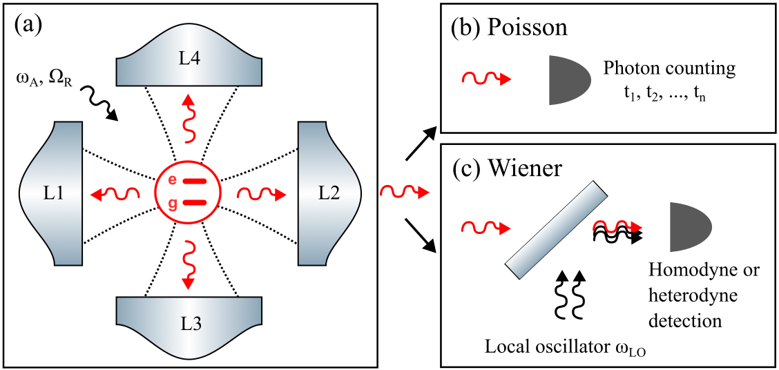
Figure 1: Schematic representation of the two main unraveling schemes. In this setup, the trapped two-state atom is illuminated in a Maltese-cross arrangement Bruno et al. (2019); Weber et al. (2006) shown in (a). The output radiation escaping a particular lens is directed to either: (b) a collection of avalanche photodetectors (APDs) producing a time-series of “click” events (Poisson-type unraveling); (c) a mixer with a strong local oscillator field, to substantiate either a homodyne ($\omega_{\rm LO}=\omega_{A}$) or a heterodyne measurement ($|\omega_{\rm LO}-\omega_{A}|\gg\gamma$) scheme (Wiener-type unraveling).

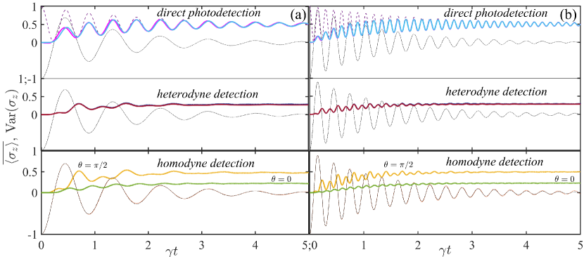
Figure 2: Linear vs. nonlinear quantum-trajectory averages for three principal unravelings. Monte-Carlo averages over $10^{4}$ realizations of the QTAV ${\rm Var}(\sigma_{z})$ plotted against the dimensionless time $\gamma t$ for a Poisson-type unraveling (direct photodetection) and two Wiener-type unravelings (homodyne and heterodyne detection) as indicated in each panel, for (a) $Y=10$ and (b) $Y=30$, with the two-level atom initialized in its ground state. The oscillatory dot-dashed curves with alternating sign in all frames depict the average inversion $\overline{\langle\sigma_{z}(t)\rangle}$. In the uppermost panels of both frames, the pink and blue curves depict ${\rm Var(\sigma_{z})}$ obtained from the perturbative treatment of the Dyson-series expansion to first order in $\gamma/\Omega$, and the moment-based equations, respectively. The latter results are indistinguishable from the Monte-Carlo simulations on the scale of the figure. The dashed curves (in purple) depict the asymptotic expression (3). For heterodyne detection, the QTAV obtained from the numerical simulations (in blue) is indistinguishable from the moment-based method results (in red). Homodyne detection is performed with the local-oscillator phase selected along the anti-squeezed and squeezed quadratures of the fluorescent field, at $\theta=0$ and $\pi/2$, respectively, corresponding to the same inversion average (brown curve overlapping with the dot-dashed).

.

By producing photon counting records, the experimenter effectively defines the environment by a particular idealization of what might lie in the path of the scattered field – a perfectly absorbing boundary. Every photon scattered by the two-state atom is then used up making a record appropriate to this environment Carmichael (1999). Other idealized environments will produce different records, and disentangle the system and environment in different ways Nha and Carmichael (2004). Quantities that are linear in the density matrix $\rho(t)$, such as averages of observables, are fully determined by the GKSL equation, and therefore are independent of the choice of the unraveling dictated by a given photodetection scheme. Going beyond the standard density-matrix formulation, in this Letter we demonstrate that evaluating an expectation value of a physical observable along a given trajectory, and performing a nonlinear operation on the obtained result, yields a quantity that allows one to distinguish different unravelings of one and the same GKSL equation.

Focusing on one Poisson (direct photodetection) and two Wiener-type unravelings (homodyne/heterodyne detection), we introduce a variance of quantum mechanical averages, visualizing the quantum jumps and the regression of fluctuations for a system observable. Taking into account common experimental limitations, we discuss the prospects of measurements of these variances in the present-day single-atom settings. Furthermore, we introduce an iterative scheme based on a truncated hierarchy of moments allowing for an approximate symbolic solution of the stochastic differential equations modeling the Poisson and Wiener processes.

Source Master Equation and linear averages.—Our starting point is the GKSL ME of resonance fluorescence, governing the unconditional evolution of the reduced system density matrix $\rho$,

$$\frac{d\rho}{dt}=\mathcal{L}\rho= -i\tfrac{1}{2}\omega_{A}[\sigma_{z},\rho]-i\Omega[e^{-i\omega_{A}t}\sigma_{+}+e^{i\omega_{A}t}\sigma_{-},\rho]$$ (1)

$$+\tfrac{\gamma}{2}(2\sigma_{-}\rho\sigma_{+}-\sigma_{+}\sigma_{-}\rho-\rho\sigma_{+}\sigma_{-}),$$

where we have neglected thermal excitation SM . In the ME (1), $\sigma_{+},\sigma_{-},\sigma_{z}$ are the raising, lowering and inversion operators (represented by Pauli matrices), respectively, for the two-level atom coherently driven on resonance by a laser field of frequency $\omega_{A}$; $\Omega_{R}=2\Omega$ is the Rabi frequency at which the two-state atom periodically cycles between its upper and lower states, and $\gamma$ is the spontaneous emission rate. The solution of the corresponding optical Bloch equations yields the following expression for the average inversion when the atom is initialized in its ground state,

$$\overline{\langle\sigma_{z}(t)\rangle}\!=\!S_{z}\!\left[1\!+\!Y^{2}e^{-\left(3\gamma/4\right)t}\!\left(\!\cosh{\delta t}\!+\!\frac{\left(3\gamma/4\right)}{\delta}\sinh{\delta t}\!\right)\right],$$ (2)

where $Y\equiv\sqrt{2}\Omega_{R}/\gamma$, $\delta\equiv\tfrac{\gamma}{4}\sqrt{1-8Y^{2}}$ and $S_{z}=-1/(1+Y^{2})$ is the steady-state inversion. Hereinafter, we denote by $\langle\cdot\rangle$ the quantum mechanical average over an individual realization. For strong driving ($Y\gg 1$) the average inversion exhibits damped oscillations at $\Omega_{R}$, relaxing to $0+\mathcal{O}(\gamma^{2}/\Omega^{2})$. Equation (2) displays a typical linear average computed directly from the ME, against which our nonlinear averages are to be compared. We now describe nonlinear averages.

Nonlinear averages beyond the density-matrix formalism.—The key difference with respect to linear averages lies in performing nonlinear operations to individual quantum mechanical averages before taking the sum over all possible realizations. A characteristic nonlinear average of the kind is the quantity ${\rm Var}(\sigma_{z})\equiv\overline{\langle\sigma_{z}(t)\rangle^{2}}-[\overline{\langle\sigma_{z}(t)\rangle}]^{2}$, which we hereinafter call quantum-trajectory-averaged variance (QTAV). We will see below how the twist from an ordinary variance highlights the explicitly open-system-character of a resonance fluorescence setup.

The results depicted in Fig. 2 substantiate the pivotal influence of the environment when collecting records of a strongly driven two-state atom and taking a sum over a collection of them. The two principal unravelings are presented in their ability to produce an ostensibly disparate ${\rm Var}(\sigma_{z})$, while the corresponding average inversion remains unchanged. Under direct photodetection Mollow (1975); Cook (1980, 1981), yielding a Poisson-type unraveling of the ME, we obtain an exact expression for ${\rm Var}(\sigma_{z})$ based on the waiting-time distribution Carmichael et al. (1989). For $\gamma t\gg 1$, the asymptotic expression for the variance, including first-order terms in $\gamma/\Omega$ of different frequencies, reads SM

$${\rm Var}(\sigma_{z})= \tfrac{1}{2}\Big{\{}1+e^{-\gamma t/2}\cos(4\Omega t)+\tfrac{\gamma}{8\Omega}e^{-\gamma t/2}[4\sin(4\Omega t)$$ (3)

$$-\sin(6\Omega t)-3\sin(2\Omega t)]+\mathcal{O}(\gamma^{2}/\Omega^{2})\Big{\}}.$$

The first observation to be made from Eq. (3) is that the amplitude of the dominant term (second term in the sum) to the QTAV – revealing a frequency doubling with respect to the inversion – is independent of $\Omega$. The variance ultimately relaxes to $1/2$, as we can see in both uppermost panels of frames (a) and (b). The asymptotic evolution to the steady state is in very good agreement with the exact Monte-Carlo simulations as well as with the perturbative treatment of the Dyson-series expansion for the variance, and the truncated hierarchy of moments produced from the adjoint Lindbladian.

Notable changes arise when one places a beam splitter and a local oscillator in the environment, and the fluorescent signal interferes with the latter before photodetection [Fig. 1(c)]: Next in line comes heterodyne detection, exemplifying a typical Wiener-type unraveling reported in the middle panels of Fig. 2. The frequency doubling is also in evidence although the contrast in the oscillations is visibly suppressed, as is the steady-state value of the variance. It is known that the light scattered by the two-level emitter is squeezed in the field quadrature that is in phase with the mean scattered field amplitude $\propto\langle\sigma_{-}(t)\rangle$ Walls and Zoller (1981); Mandel (1982). The bottom panel in each frame shows that the QTAV responds differently to the detection of the squeezed vs. the direction of the antisqueezed quadrature of the fluorescent field, i.e., along an axis perpendicular to the equator of the Bloch sphere where quantum fluctuations are redistributed among the quadratures.

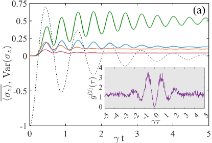
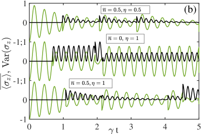
Figure 3: Experimental limitations and decay of “conditional” coherence. (a) Monte-Carlo average over $10^{4}$ realizations of the QTAV ${\rm Var}(\sigma_{z})$ plotted against the dimensionless time $\gamma t$ for the ideal case $\overline{n}=0,\eta=1$ (in green), $\overline{n}=0,\eta=0.5$ (in blue), $\overline{n}=1,\eta=1$ (in orange), and $\overline{n}=1,\eta=0.5$ (in red). The dashed curve depicts $\overline{\langle\sigma_{z}(t)\rangle}$ in the ideal case. The inset shows a typical experimentally obtained intensity correlation function $g^{(2)}(\tau)$ of the scattered light from the two-level emitter [using the setup of Fig. 1(a)], for $\Omega\approx 3\gamma$ and in the presence of significant detuning from the drive ($\approx-3\gamma$). The detection efficiency from a single lens is $\eta\approx 0.25\%$ SM (b) Monte-Carlo average over two realizations for the atomic inversion, $\overline{\langle\sigma_{z}(t)\rangle}$ (in green) and ${\rm Var}(\sigma_{z})$ (in black) for the values of $\overline{n},\eta$ indicated in each textbox.

.

Ensemble moments and adjoint Lindbladian.—To provide some analytical grounding to the formation of the QTAV, we will delineate a method akin to the optical Bloch equations extended to account for nonlinear averages. The contributions from the Itô corrections to the ensemble moments can be found easily in the Heisenberg picture Keys (2022). Under the Poisson unraveling for an observable $A$ Barchielli and Belavkin (1991) (we denote $\langle A(t)\rangle$ by $\langle A\rangle_{t}$):

$$d\left\langle A\right\rangle_{t}=\left\langle\mathcal{L}^{\dagger}[A]\right\rangle_{t}dt+\left(\dfrac{\left\langle\sigma_{+}A\sigma_{-}\right\rangle_{t-}}{\left\langle\sigma_{+}\sigma_{-}\right\rangle_{t-}}-\left\langle A\right\rangle_{t_{-}}\right)d\widetilde{N}(t),$$ (4)

where $\widetilde{N}$ is the compensated Poisson process, $d\widetilde{N}=dN-\gamma\left\langle\sigma_{+}\sigma_{-}\right\rangle_{t}dt$, with a future pointing differential of expected value zero. This means that the ensemble average, here denoted by $\mathbb{E}$ for readability, is just

$$d\mathbb{E}\left\langle A\right\rangle_{t}=\mathbb{E}\left\langle\mathcal{L}^{\dagger}[A]\right\rangle_{t}dt,$$

which is the Heisenberg unraveling of the ME. It is useful to consider this equation for a Hilbert-Schmidt basis $X_{i}$ for the space of observables. Call the quantum expectation $x_{i}=\left\langle X_{i}\right\rangle$. Thus each observable $A$ has a corresponding vector $a$ such that $\left\langle A\right\rangle=(a,x)$. If we use the basis corresponding to the three Pauli matrices and the identity, all normalized in the Hilbert-Schmidt norm, then the vector for $A=\sigma_{z}$ is $a=(0,0,0,\sqrt{2})$. Since $a$ is just a constant vector, generally we have that $\mathbb{E}\left\langle A\right\rangle=\mathbb{E}(a,x)=(a,\mathbb{E}x)$ and the square of the quantum expectation becomes $\left\langle A\right\rangle^{2}=\sum_{ij}a_{i}a_{j}x_{i}x_{j}$ so that $\mathbb{E}\left\langle A\right\rangle^{2}=\sum_{ij}a_{i}a_{j}\mathbb{E}x_{i}x_{j}$ and so to see how the ensemble average of square of the quantum expectation evolves in time it is necessary to know how $\mathbb{E}x_{i}x_{j}$ evolves. In the Poisson case, we obtain

$$d\mathbb{E}x_{i}x_{j}=\mathbb{E}\left(x_{i}\left\langle\mathcal{L}^{\dagger}[X_{j}]\right\rangle_{t}dt+\left\langle\mathcal{L}^{\dagger}[X_{i}]\right\rangle_{t}x_{j}dt\right)+$$

$$\mathbb{E}\left(\dfrac{\left\langle\sigma_{+}X_{i}\sigma_{-}\right\rangle_{t}}{\left\langle\sigma_{+}\sigma_{-}\right\rangle_{t}}-x_{i}\right)\left(\dfrac{\left\langle\sigma_{+}X_{j}\sigma_{-}\right\rangle_{t}}{\left\langle\sigma_{+}\sigma_{-}\right\rangle_{t}}-x_{j}\right)$$

$$\times\left\langle\sigma_{+}\sigma_{-}\right\rangle_{t}dt=\mathbb{E}\Big{(}x_{i}(u^{j},x)+(u^{i},x)x_{j}$$

$$+\dfrac{1}{(l,x)}\left((v^{i},x_{i})-x_{i}(l,x)\right)\left((v^{j},x)-x_{j}(l,x)\right)\Big{)}dt,$$

using the fact that $d\widetilde{N}d\widetilde{N}=dN$ with the rate of the Poisson process being $\gamma\left\langle\sigma_{+}\sigma_{-}\right\rangle_{t}dt$ and in the last line using $u^{j}$ as the vector corresponding to $\mathcal{L}^{\dagger}[X_{j}]$, $l$ as $\sigma_{+}\sigma_{-}$, and $v^{j}$ as $\sigma_{+}X_{j}\sigma_{-}$. This is an ordinary differential equation which however does not close since it requires higher order moments such as $\mathbb{E}x_{i}x_{j}x_{k}$. Again, using the Itô product rule we can calculate the equation for the higher order moments to obtain a system of ordinary differential equations which still do not close. We can repeat this procedure to arbitrarily high order but at some point we have to truncate. It can be shown that this truncation is linear in the moments, which allows us to solve the system using traditional methods of solving linear systems of ODEs. The Wiener case Barchielli and Belavkin (1991); Gisin and Percival (1992) can be similarly approximately solved by using the Heisenberg equation Keys (2022)

$$d\left\langle A\right\rangle_{t}\!=\!\left\langle\mathcal{L}^{\dagger}[A]\right\rangle_{t}dt\!+\!\left(\sqrt{\gamma}\left\langle A(\sigma_{-}-\left\langle\sigma_{-}\right\rangle_{t})\right\rangle\frac{dW(t)}{\sqrt{2}}\!+\!{\rm h.c.}\right),$$

where $W$ is a complex Wiener process. Solutions to these kind of truncated systems of equations for the two principal unravelings are depicted in Fig. 2, in very good agreement with the Dyson-expansion method and Monte-Carlo averages.

Direct photodetection revisited and compromised.—Having laid out an operational approach to distinguish the different unravelings, let us return to direct photodetection and discuss the most commonly encountered limitations in an actual experiment, where the density matrix cannot be unraveled into a pure-state ensemble, in which we would have a conditional wavefunction obeying a Schrödinger equation with a non-Hermitian Hamiltonian. This happens for a limited detector efficiency $\eta<1$ and/or a surrounding bath with appreciable thermal excitation $\overline{n}$ SM .

Figure 3 testifies to the rapid degradation of ${\rm Var}(\sigma_{z})$ as we move away from a pure-state description of the conditional dynamics. The QTAV responds to quantum jumps taking place in the course of individual realizations. This is evident from Fig. 3(b) where ${\rm Var}(\sigma_{z})$ remains zero until a spontaneous-emission event occurs in a pair of realizations. For an imperfect detector or for a thermally excited bath, the regression of fluctuations following a jump is damped. The decay concerns the coherent part of the evolution between spontaneous emissions, at a rate much faster than $\gamma$, for typical experimental parameters where $\eta\ll 1$.

The inset shows the intensity correlation function $g^{(2)}(\tau)\propto(1+\langle\sigma_{z}(\tau)\rangle_{\rho(0)=|\downarrow\rangle\langle\downarrow|})$ obtained from real experimental data based on the setup of Fig. 1(a). Since the intensity correlation of the scattered light reflects a nonexclusive probability of photocounting coincidences, the limited detector efficiency can be counterbalanced by increasing the number of photon “clicks” $N$ in the course of a long experimental run. Indeed, we have concluded that the signal-to-noise ratio for $g^{(2)}(\gamma\tau\gg 1)$ in a window about one inverse of the coherence time scales with $\sqrt{N}$ SM . This allows the determination of ${\rm Var}(\sigma_{z})$ from single realizations as low as $10^{-3}$, the order of magnitude Monte-Carlo simulations indicate for $\eta\lesssim 0.05$. This order of magnitude can be increased using high numerical aperture collection systems Bruno et al. (2019); Natarajan et al. (2012) and efficient single-photon detectors Chou et al. (2017).

Conclusions and outlook.—In summary, we have expanded upon the fundamental concept of the variance in quantum mechanics going beyond the conventional density-matrix formulation. The different environments devised to collect the output of an open quantum system show up in a markedly different response of a quantity where nonlinear operations are performed to individual realizations prior to averaging over their ensemble. This is in contrast to linear observable averages where the complementary measurement strategies all abide by the predictions of the GKSL equation, and multi-time correlations – such as the intensity correlation function – are obtained via the quantum regression formula. Following our strategy, we need to set the initial point for two copies of the system (here a ground-state reset for direct photodetection) and then post-select the trajectories in such a way that the photocounting record is the same with satisfactory accuracy. Ergo, one gains, in principle, the ability to characterize the experiment’s power to collapse the wavefunction and add information to the memory carried by a state conditioned on all events that have taken place along a single trajectory.

Supplementary Information

In the supplementary material, we first detail the calculation of the quantum-trajectory-averaged variance ${\rm Var}(\sigma_{z})$ for the Poisson-type unraveling, via the Dyson-series expansion of the conditional reduced system density operator. We derive exact and approximate results, the latter in the limits of strong and weak driving where asymptotic expressions can be obtained. Secondly, we expand on the generality of the moment-based method applicable to the two principal types of unraveling (Poisson and Wiener). We also connect the quadrature amplitude squeezing encountered in resonance fluorescence to ${\rm Var}(\sigma_{z})$. Finally, we take into account experimental imperfections and discuss a strategy to determine nonlinear averages in an exemplary and pioneering system of a single trapped fluorescing ⁸⁷Rb atom whose output radiation is collected by four partially transmitting mirrors in a Maltese-cross arrangement.

.1 Introduction: record making and complementarity

The theory of quantum trajectories ultimately attempts to describe the energy exchange between light and atoms, given both the quantum and wave aspects of light. The exchange must be described in a background where the quantum indicates discontinuity while the wave indicates continuity, and quantum trajectories fit both aspects in an evolution over time N. Bohr and Slater (1924). They employ the random stochastic processes and a formal generalization of the quantum jump to account for coherence Hegerfeldt (2009); Carmichael (1993). Both event-enhanced quantum theory Blanchard and Jadczyk (1995) and consistent histories Omnès (1994) emphasize the need to attach meaningful time series of real numbers to a quantum evolution. The series are the records obtained in the scattering scenario of a quantum optical experiment.

By producing photon counting records, we effectively define the environment by a particular idealization of what might lie in the path of the scattered field – a perfectly absorbing boundary. Every photon scattered by the two-state atom is then used up making a record appropriate to this environment. Other idealized environments will produce different records, and disentangle the system and environment in different ways Nha and Carmichael (2004). There are many different environments that might, in fact, be encountered by the scattered field, all consistent with the master equation (ME). Different environments correspond to mutually exclusive methods of record making, since every photon produces one and only one happening. Each idealized environment defines a self-consistent pure-state unraveling. This is how quantum-trajectory theory encounters Bohr’s complementarity. Apart from direct photodetection, there is another particularly important way of making records. It introduces a beam splitter and a local oscillator into the environment, and after the beam splitter every photon is counted. The scheme of homodyne and heterodyne detection uses interference to unveil aspects of the scattering process associated with a wave amplitude and a spectrum Carmichael (1999). In the sections that follow, we will visit these complementary unravelings of the ME of resonance fluorescence, when producing the single realizations which make the quantum-trajectory-averaged variance (QTAV).

.2 Resonance fluorescence and waiting-time distribution

We work with the paradigmatic system of resonance fluorescence, comprising a coherently driven two level atom (whose ground and excited states are denoted by $\ket{\downarrow}$ and $\ket{\uparrow}$, respectively) immersed in the vacuum reservoir. The derivation of the photoelectron counting distribution by Mollow Mollow (1975) and Cook Cook (1980, 1981) is based on a hierarchy of equations that yield the probabilities for finding $n$ photons in the multimode fluorescent field. These equations were then used in the analysis of quantum jumps Zoller et al. (1987).

In such a system, the trajectories themselves are Markovian (as well as the averaged dynamics conforming to the Gorini-Kossakowski-Sudarshan-Lindblad (GKSL) equation), since the dynamical evolution is reset to the same state following a quantum jump. As usual, we denote by $\sigma_{-}$ and $\sigma_{+}$ the lowering and raising system operators, respectively, $\Omega$ is the Rabi frequency which is taken real without loss of generality, and $\gamma$ is the spontaneous decay rate. The conditional evolution of the system state under direct photodetection (with unit detector efficiency) is described by the ME Gorini et al. (1976); Lindblad (1976)

$$\dot{\rho}_{c}=\mathcal{L}\rho_{c}=(\ell+J)\rho_{c},$$ (S.1)

where in the interaction picture we may write

$$\ell\rho_{c}=[1/(i\hbar)][H,\rho_{c}]-\frac{\gamma}{2}\left(\sigma_{+}\sigma_{-}\rho_{c}+\rho_{c}\sigma_{+}\sigma_{-}\right)=[1/(i\hbar)](H_{\rm eff}\rho_{c}-\rho_{c}H_{\rm eff}^{\dagger}),$$ (S.2)

in which $H_{\rm eff}$ is a non-Hermitian Hamiltonian. It describes a continuous evolution of the system state with decreasing norm, between randomly occurring spontaneous emission events

$$H_{\rm eff}=\hbar\Omega(\sigma_{+}+\sigma_{-})-i\hbar(\gamma/2)\sigma_{+}\sigma_{-}.$$ (S.3)

The continuous evolution is interrupted by quantum jumps accounted for by the action of the super-operator

$$J\rho_{c}=\gamma\sigma_{-}\rho_{c}\sigma_{+}.$$ (S.4)

The above jump superoperator projects the system state to the ground state ($\ket{\downarrow}$), captures the aftermath of a photon emission. The time $\tau$ lapsed (often called waited time) between successive emissions is governed by the waiting-time distribution $w(\tau)$. This exclusive probability density function of the time intervals $\tau$ between two consecutive jumps, is given by the expression

$$w\left(\tau\right)={\rm Tr}\left(Je^{\ell\tau}(\left|\downarrow\right\rangle\left\langle\downarrow\right|)\right)=\gamma|\langle\uparrow|e^{[1/(i\hbar)]H_{\rm eff}\tau}|\downarrow\rangle|^{2}=\exp\left(-\frac{\gamma\tau}{2}\right)\frac{\gamma\Omega^{2}}{\mu^{2}}\sin^{2}{\left(\mu\tau\right)},$$ (S.5)

with $\mu=\frac{1}{2}\sqrt{4\Omega^{2}-\left(\frac{\gamma}{2}\right)^{2}}$. The waiting-time distribution forms the basis of the quantum-trajectory description of resonance fluorescence in direct photodetection Carmichael et al. (1989), as we will see in the following sections.

.3 Dyson expansion and quantum-trajectory formulation in direct photodetection

The solution of the ME (S.1) can be expressed by means of the Dyson expansion Carmichael (1993); Srinivas and Davies (1981); Zoller et al. (1987); Dum et al. (1992) as follows

$$\rho_{c}\left(t\right)=e^{\ell t}\rho_{c}\left(0\right)+\int_{0}^{t}e^{\ell\left(t-t_{1}\right)}Je^{\ell t_{1}}\rho_{c}\left(0\right)\mathrm{d}t_{1}+\int_{0}^{t}\int_{0}^{t_{2}}e^{\ell\left(t-t_{2}\right)}Je^{\ell\left(t_{2}-t_{1}\right)}Je^{\ell t_{1}}\rho_{c}\left(0\right)\mathrm{d}t_{2}\mathrm{d}t_{1}+...$$ (S.6)

This form of the solution is very useful to see what an average over all the possible different quantum trajectories is made of, i.e. track the conditioned evolution paths. For example, the first term of the RHS describes a trajectory with no jumps at all. The second term describes all the possible trajectories with one jump at any time instant during the evolution, and so on. In fact, assuming $\rho\left(0\right)=\left|\downarrow\right\rangle\left\langle\downarrow\right|$, this solution can be recast in the explicit form of an average

$$\rho_{c}\left(t\right)=\sum_{n=0}^{\infty}\int_{0}^{t}\int_{0}^{t_{n}}...\int_{0}^{t_{2}}dt_{n}...dt_{1}\frac{e^{\ell\left(t-t_{n}\right)}\left(\left|\downarrow\right\rangle\left\langle\downarrow\right|\right)}{p_{0}(t-t_{n})}p_{n}(t,t_{1},t_{2},...,t_{n}),$$ (S.7)

where

$$p_{n}(t,t_{1},t_{2},...,t_{n})=p_{0}(t-t_{n})w(t_{n}-t_{n-1})...\;w(t_{2}-t_{1})w(t_{1})$$ (S.8)

is the exclusive probability density for realizing one particular trajectory with $n$ jumps at times $t_{1},t_{2},...,t_{n}$ and no jumps between $t_{n}$ and $t$ Breuer and Petruccione (2002). Here,

$$p_{0}(t-t_{n})={\rm Tr}(e^{\ell\left(t-t_{n}\right)}\left|\downarrow\right\rangle\left\langle\downarrow\right|)=e^{-\frac{\gamma(t-t_{n})}{2}}\left[\frac{\Omega^{2}}{\mu^{2}}-\frac{\gamma^{2}}{16\mu^{2}}\cos{\left(2\mu\left(t-t_{n}\right)\right)}+\frac{\gamma}{4\mu}\sin\left(2\mu\left(t-t_{n}\right)\right)\right]$$ (S.9)

is the null measurement probability density, from the time $t_{n}$ when the last jump was recorded to the final time $t$.

.3.1 Ensemble average of nonlinear functions of quantum mechanical expected values

Using the previously derived expressions, one can obtain the following formula for the ensemble average of the quantum mechanical expected value of an operator $O$:

$$\overline{\braket{O(t)}}={\rm Tr}\left(O\rho_{c}\left(t\right)\right)=\sum_{n=0}^{\infty}\int_{0}^{t}\int_{0}^{t_{n}}...\int_{0}^{t_{2}}dt_{n}...dt_{1}\frac{{\rm Tr}\left(Oe^{\ell\left(t-t_{n}\right)}\left|\downarrow\right\rangle\left\langle\downarrow\right|\right)}{p_{0}(t-t_{n})}p_{n}(t,t_{1},t_{2},...,t_{n}).$$ (S.10)

Here, the overbar denotes the ensemble average over all the possible trajectories and the brackets for the quantum mechanical expected value of each one of them. It is the common average obtained from the ME. Based on Eq. (S.10) we can construct a nonlinear average where the single-trajectory quantum mechanical average is raised to some power, i.e., after effecting a nonlinear operation in a post-selection process

$$\overline{\braket{O(t)}^{m}}=\sum_{n=0}^{\infty}\int_{0}^{t}\int_{0}^{t_{n}}...\int_{0}^{t_{2}}dt_{n}...dt_{1}O_{m}\left(t-t_{n}\right)w(t_{n}-t_{n-1})...\;w(t_{2}-t_{1})w(t_{1}),$$ (S.11)

with

$$O_{m}\left(t\right)=\frac{\left[{\rm Tr}\left(Oe^{\ell t}\left(\left|\downarrow\right\rangle\left\langle\downarrow\right|\right)\right)\right]^{m}}{p_{0}^{m-1}(t)},$$ (S.12)

a considerably simplified form given that after the last ($n$) jump the wavefunction has collapsed to $\ket{\downarrow}$ (the individual trajectory is Markovian).

We remark that Eq. (S.11) is an expression which cannot be obtained from the ME without the quantum trajectories point of view of the system evolution. Note that the expression for $\overline{\braket{O(t)}^{m}}$ is just a sum over successive convolutions:

$$\overline{\braket{O(t)}^{m}}=\sum_{n=0}^{\infty}O_{m}(t-t_{n})\ast\Bigl{\{}w\left(t_{n}-t_{n-1}\right)...\ast\bigl{[}w\left(t_{2}-t_{1}\right)\ast w\left(t_{1}\right)\bigr{]}\Bigr{\}}.$$ (S.13)

Now, applying the Laplace transform (which we denote as an upper tilde), we obtain the following expression for the ensemble average of the nonlinear quantum mechanical expected value:

$$\widetilde{\overline{\braket{O(t)}^{m}}}=\sum_{n=0}^{\infty}\widetilde{O_{m}}\left(z\right)\widetilde{w}^{n}\left(z\right)=\frac{\widetilde{O_{m}}\left(z\right)}{1-\widetilde{w}\left(z\right)}.$$ (S.14)

.3.2 Characteristic examples of nonlinear averages obtained via the Dyson expansion

To illustrate the method, we chose the Pauli operator $\sigma_{z}$ and as a nonlinear function of the quantum mechanical average we select the square, i.e., $m=2$. In this case,

$$\sigma_{z_{\;m=2}}(t)=\frac{\left[{\rm Tr}\left(\sigma_{z}e^{\ell t}\left(\left|\downarrow\right\rangle\left\langle\downarrow\right|\right)\right)\right]^{2}}{p_{0}(t)},$$ (S.15)

with the denominator given by Eq. (S.9). Working on the numerator, we obtain the exact expression:

$$\Bigl{(}{\rm Tr}\left(\sigma_{z}e^{\ell t}\left(\left|\downarrow\right\rangle\left\langle\downarrow\right|\right)\right)\Bigr{)}^{2}=e^{-\gamma t}\left\{\frac{1}{2}+\frac{\gamma^{2}}{32\mu^{2}}+\frac{1}{2}\left[1-\frac{\gamma^{2}}{16\mu^{2}}\right]\cos(4\mu t)+\frac{\gamma}{4\mu}\sin(4\mu t)\right\},$$ (S.16)

identifying a dominant oscillatory term of frequency $4\mu$. A frequency mixing, however, is bound to arise due to the denominator $p_{0}(t)$, albeit scaled by powers of $\gamma/\Omega$.

The above observation brings us to the strong-driving limit, $Y\gg 1$, with $Y\equiv 2\sqrt{2}\Omega/\gamma$. Neglecting second-order terms in $(\gamma/\Omega)^{2}\ll 1$ we write $\mu\approx\Omega$; taking the Laplace transform of $\sigma_{z_{\;m=2}}(t)$, multiplying by $1/[1-\tilde{w}(z)]$ and going back to the time domain yields the following approximate form:

$$\begin{split}\overline{\braket{\sigma_{z}(t)}^{2}}&\approx\frac{1}{2}+\frac{1}{4}e^{-\frac{3}{4}\gamma t}\Bigl{[}C_{1}\cos{(C_{\Omega}t)}+C_{2}\sin{(C_{\Omega}t)}\Bigr{]}+\\ &+\frac{1}{4}e^{-\frac{\gamma}{2}t}\Bigl{[}C_{3}\cos{(4\Omega t)}+C_{4}\sin{(4\Omega t)}+C_{5}\cos{(6\Omega t)}+C_{6}\sin{(6\Omega t)}\Bigr{]}.\end{split}$$ (S.17)

The coefficients $C_{1},...,C_{6}$ depend nonlinearly on the ratio $\gamma/\Omega$, while $C_{\Omega}\approx 2\Omega$, in agreement with the occurrence of the pair of eigenvalues with real part $-3\gamma/4$ (distinct from the vertical line at $-\gamma/2$) shown in Fig. S.1.

In the case of $\sigma_{y}$, we find that the form of the solution is the same, and only the coefficients $C_{1}-C_{6}$ change. On the other hand, for the case of $\sigma_{x}$, the solution has an easier form, but it is different from zero only in the presence of a finite detuning $\Delta$ between the laser drive and the atomic resonance.

.3.3 Asymptotic results for strong and weak drive in the long-time limit

Let us now consider the long-time limit of the QTAV from the perspective of the final-value theorem in the Laplace Transform. We are still working under $Y\gg 1$ (with $\mu\approx\Omega$). We then obtain

$$\Bigl{(}{\rm Tr}\left(\sigma_{z}e^{\ell t}\left(\left|\downarrow\right\rangle\left\langle\downarrow\right|\right)\right)\Bigr{)}^{2}=\tfrac{1}{2}e^{-\gamma t}[1+\cos(4\Omega t)]+\mathcal{O}(\gamma/\Omega),$$ (S.18)

while $p_{0}(t)\approx e^{-\gamma t/2}+\mathcal{O}(\gamma/\Omega)$. As we have seen in the previous section, this leaves us to leading order with a damped oscillatory term $e^{-\gamma t/2}\cos^{2}(2\Omega t)+\mathcal{O}(\gamma/\Omega)$, “screened” by a convolution kernel, the inverse Laplace Transform of $[1-\tilde{w}(z)]^{-1}$. Applying the final-value theorem, where $[1-\tilde{w}(z)]^{-1}\approx(z+\gamma/2)/z$ for $z\sim\gamma$, yields $1/2+\mathcal{O}(\gamma^{2}/\Omega^{2})$ for the long-time limit of ${\rm Var}(\sigma_{z})$. Given that $S_{z}\equiv\langle\sigma_{z}\rangle_{\rm ss}=0+\mathcal{O}(\gamma^{2}/\Omega^{2})$, the asymptotic expression for the time-evolving variance–including first-order terms in $\gamma/\Omega$ of different frequencies–becomes (for $t\gg\gamma^{-1}$)

$$\boxed{{\rm Var}(\sigma_{z})=\tfrac{1}{2}\left\{1+e^{-\gamma t/2}\cos(4\Omega t)+\tfrac{\gamma}{8\Omega}e^{-\gamma t/2}[4\sin(4\Omega t)-\sin(6\Omega t)-\sin(2\Omega t)]-\tfrac{\gamma}{4\Omega}e^{-\gamma t/2}\sin(2\Omega t)\right\}+\mathcal{O}(\gamma^{2}/\Omega^{2}),}$$ (S.19)

which makes Eq. (3) of the main text, one of our central results. Although limited in its applicability, is shows that all oscillatory terms decay with the same rate, $\gamma/2$, consistent with the eigenvalue distribution plotted in Fig. S.1. Comparing with Eq. (S.17), we expect that the coefficient $C_{3}$ does not scale with $\gamma/\Omega$ for $Y\gg 1$ but approaches a constant value. Indeed, we find that $C_{3}\approx 2$, while $C_{4}\sim 1/Y$. At the same time, the initial-value theorem gives ${\rm Var}(\sigma_{z})(t\to 0^{+})=0+\mathcal{O}(\gamma^{2}/\Omega^{2})$, which we have also numerically confirmed (see Fig. 2 of the main text).

In the opposite limit, $\Omega/\gamma\ll 1$, we use $\mu/\gamma=i\frac{1}{4}+\mathcal{O}((\Omega/\gamma)^{2})$. This yields

$$\Bigl{(}{\rm Tr}\left(\sigma_{z}e^{\ell t}\left(\left|\downarrow\right\rangle\left\langle\downarrow\right|\right)\right)\Bigr{)}^{2}=e^{-\gamma t}[\cosh(\gamma t)+\sinh(\gamma t)],$$ (S.20)

and

$$p_{0}(t)=e^{-\gamma t/2}[\cosh(\gamma t/2)+\sinh(\gamma t/2)],$$ (S.21)

to leading order in $\Omega/\gamma$. At the same time, from Eq. (S.11) we see that $\tilde{w}(z)\to 1$ for $z\to 0$, which means that we cannot use the Laplace transform and the geometric series expansion of $[1-\tilde{w}(z)]^{-1}$. Instead, we allow at most one jump in the approach to the steady state ($n=1$) and we directly appeal to the Dyson expansion in the time domain. The asymptotic expression for the variance, then, reads:

$$\boxed{{\rm Var}(\sigma_{z})=e^{-\gamma t/2}\frac{\cosh{\gamma t}+\sinh{\gamma t}}{\cosh{(\gamma t/2)}+\sinh{(\gamma t/2)}}-1+\mathcal{O}((\Omega/\gamma)^{2})=0+\mathcal{O}((\Omega/\gamma)^{2}).}$$ (S.22)

In fact, Monte-Carlo simulations show that ${\rm Var}(\sigma_{z})\sim 10^{-6}$ for $\gamma/\Omega=56$.

.4 The moment-based method and the truncated hierarchy of equations: Poisson- and Wiener-type unraveling

There are two principal unravelings which define the evolution of the conditioned state vector $\ket{\psi_{c}}=\ket{\psi_{c}(t)}$. One is driven by Wiener noise Barchielli and Belavkin (1991); Gisin and Percival (1992) (in this section we set $\hbar=1$ and denote $\langle A(t)\rangle$ by $\langle A\rangle_{t}$)

$$d\ket{\psi_{c}}=-iH\ket{\psi_{c}}dt+ \sum_{i}\left(\left\langle L_{i}^{\dagger}\right\rangle_{t}L_{i}-\frac{1}{2}L^{\dagger}_{i}L_{i}-\frac{1}{2}|\left\langle L_{i}\right\rangle_{t}|^{2}\right)\ket{\psi_{c}}dt$$

$$+\frac{1}{\sqrt{2}}\sum_{i}\left(L_{i}-\left\langle L_{i}\right\rangle_{t}\right)\ket{\psi_{c}}dW_{i}(t),$$ (S.23)

where $W_{i}$ is a complex Wiener process with Itô rule $dW_{i}^{*}dW_{j}=dW_{i}dW_{j}^{*}=2\delta_{ij}dt$ and all others zero. The other unravelling is driven by Poisson noise Barchielli and Belavkin (1991),

$$d\ket{\psi_{c}}=-\bigg{(}iH +\frac{1}{2}\sum_{i}L_{i}^{\dagger}L_{i}-\left\langle L_{i}^{\dagger}L_{i}\right\rangle_{t}\bigg{)}\ket{\psi_{c}}dt$$

$$+\sum_{i}\left(\dfrac{L_{i}}{\langle L_{i}^{\dagger}L_{i}\rangle_{t-}^{1/2}}-I\right)\ket{\psi_{t-}}dN_{i}(t),$$ (S.24)

where $N_{i}$ are real Poisson processes with Itô rule $dN_{i}dN_{j}=\delta_{ij}dN_{i}$ and $dN_{i}dt=0$.

We can derive the evolution of the expectation of an observable $A$ by using the Itô product formula Keys (2022), $d\left\langle A\right\rangle=d\left\langle\psi_{c}|A|\psi_{c}\right\rangle=(d\bra{\psi_{c}})A\ket{\psi_{c}}+\bra{\psi_{c}}A(d\ket{\psi_{c}})+(d\bra{\psi_{c}})A(d\ket{\psi_{c}})$. The resulting equations are

$$d\left\langle A\right\rangle_{t}=\left\langle\mathcal{L}^{\dagger}[A]\right\rangle_{t}dt+\dfrac{1}{\sqrt{2}}\left[\sum_{j}\left\langle A(L_{j}-\left\langle L_{j}\right\rangle)\right\rangle_{t}dW_{j}(t)+h.c.\right]$$ (S.25)

and

$$d\left\langle A\right\rangle_{t}=\left\langle\mathcal{L}^{\dagger}[A]\right\rangle_{t}dt+\sum_{j}\left(\dfrac{\left\langle L_{j}^{\dagger}AL_{j}\right\rangle_{t-}}{\left\langle L_{j}^{\dagger}L_{j}\right\rangle_{t-}}-\left\langle A\right\rangle_{t-}\right)d\widetilde{N}_{j},$$ (S.26)

where $d\widetilde{N}_{j}=dN_{j}-\left\langle L_{j}^{\dagger}L_{j}\right\rangle_{t}dt$ is the compensated Poisson process (which in the main text assumed the form $d\widetilde{N}=dN-\gamma\left\langle\sigma_{+}\sigma_{-}\right\rangle_{t}dt$).

Let us denote by $X_{i}$ the basis operators of the space of observables, with $x_{i}=\left\langle X_{i}\right\rangle_{t}$. In this basis the operators $A$ are described by vectors $a$, with $a_{i}=\mbox{Tr}[A^{\dagger}X_{i}]$ so that expectations become inner products $\left\langle A\right\rangle_{t}=(a,x)$. Powers of quantum expectations become powers of inner products and thus if the ensemble average is then taken of these powers, the problem of describing their evolution reduces to finding the evolution of moments, i.e. terms like $\mathbb{E}x_{i}x_{j}x_{k}$. Using equations S.25 and S.26, we can write the evolution equations of $x_{i}$ as

$$dx_{i}=(u^{i},x)dt+\sum_{j}f^{i}_{j}dW_{j}+f^{i*}_{j}dW_{j}^{*}$$ (S.27)

in the Wiener case with $u^{i}$ the vector corresponding to $\mathcal{L}[X_{i}]$ and $f^{i}_{j}=(f^{i}_{j})_{t}=\left\langle X_{i}(L_{j}-\left\langle L_{j}\right\rangle)\right\rangle_{t}$. In the Poisson case we can similarly write

$$dx_{i}=(u^{i},x)dt+\sum_{j}g^{i}_{j}d\widetilde{N}_{j},$$ (S.28)

with $g^{i}_{j}=(g^{i}_{j})_{t}=\dfrac{1}{\left\langle L_{j}^{\dagger}L_{j}\right\rangle_{t}}\left(\left\langle L_{j}^{\dagger}X_{i}L_{j}\right\rangle_{t}-\left\langle L_{j}^{\dagger}L_{j}\right\rangle_{t}\left\langle X_{i}\right\rangle_{t}\right)$. To calculate the evolution of terms like $\mathbb{E}x_{i}x_{j}x_{k}$, we apply the Itô product formula iteratively to get $d(x_{i}x_{j}x_{k})=(dx_{i})x_{j}x_{k}+x_{i}d(x_{j}x_{k})+dx_{i}d(x_{j}x_{k})$, then take the expectation so that all martingale terms cancel out. In the Poisson case we use the fact that for a Poisson integral

$$\mathbb{E}\int_{0}^{t}f(s)dN_{j}(s)=\mathbb{E}\int_{0}^{t}f(s)\left\langle L_{j}^{\dagger}L_{j}\right\rangle_{s}ds,$$ (S.29)

which gives us license to replace $dN_{j}(t)$ with $\left\langle L_{j}^{\dagger}L_{j}\right\rangle_{t}dt$.

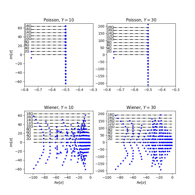
Figure S.1: Eigenvalues of the dynamical matrix $M$ corresponding to the Poisson and Wiener-type unravelings for $Y=10,30$, as indicated on top of each frame. For a Wiener-type unraveling we note that, as $Y$ grows, the spectrum of $M$ aligns better with integer multiples of the Rabi frequency $\Omega_{R}=2\Omega$.

Applying these rules leads to very simple combinatorial expressions for the evolution of moments. In the Wiener case, for the second moment we have

$$d\mathbb{E}x_{i}x_{j}=\mathbb{E}\left[(u^{i},x)x_{j}+x_{i}(u^{j},x)+\sum_{k}f^{i*}_{k}f^{j}_{k}+f^{i}_{k}f_{k}^{j*}\right]dt.$$ (S.30)

Due to the structure of the Itô product formula, simple combinatorial patterns arise for higher moments:

$$d\mathbb{E}x_{i_{1}}\cdots x_{i_{n}} =\mathbb{E}\sum_{j=1}^{n}(u^{i_{j}},x)x_{i_{1}}\cdots\hat{x}_{i_{j}}\cdots x_{i_{n}}dt+$$ (S.31)

$$\mathbb{E}\sum_{k}\sum_{\sigma\in C_{2}}f^{\sigma(i_{1})}_{k}f^{\sigma(i_{2})*}_{k}x_{\sigma(i_{3})}\cdots x_{\sigma(i_{n})}dt,$$

where $C_{k}$ is the set $\{i_{1},\ldots,i_{n}\}$ choose $k$ and hat denotes omission. For the Poisson case the pattern is a bit more complex. If $l_{k}$ denotes the vector representing $L_{k}^{\dagger}L_{k}$, then we have for the quadratic case

$$d\mathbb{E}x_{i}x_{j}=\mathbb{E}\left[(u^{i},x)x_{j}+x_{i}(u^{j},x)+\sum_{k}g_{k}^{i}g_{k}^{j}(l^{k},x)\right]dt$$ (S.32)

and for the general case

$$d\mathbb{E}x_{i_{1}}\cdots x_{i_{n}} =\mathbb{E}\left[\sum_{j=1}^{n}(u^{i_{j}},x)x_{i_{1}}\cdots\hat{x}_{i_{j}}\cdots x_{i_{n}}\right.+\sum_{k}\sum_{\sigma\in C_{2}}g_{k}^{\sigma(i_{1})}g_{k}^{\sigma(i_{2})}x_{\sigma(i_{3})}\cdots x_{\sigma(i_{n})}(l^{k},x)$$ (S.33)

$$\left.+\sum_{k}\sum_{\sigma\in C_{3}}g_{k}^{\sigma(i_{1})}g_{k}^{\sigma(i_{2})}g_{k}^{\sigma(i_{3})}x_{\sigma(i_{4})}\cdots x_{\sigma(i_{n})}(l^{k},x)+\cdots+\sum_{k}g_{k}^{i_{1}}\cdots g_{k}^{i_{n}}(l_{k},x)\right]dt,$$

where in this case there is a summation for every set $C_{l}$, $l=1,\ldots,n$, each having $l$ many $g^{\sigma(i)}_{k}$ terms.

In both cases, the evolution is described by a linear equation in the moments (even in the Poisson case where a polynomial division must be performed which has remainder $0$), however the equations for the evolution of a moment generally contain higher order moments so the equations do not close. One way to handle this is to truncate at some high order and not consider the evolution of terms beyond that order. Then the system of equations can be solved using standard methods. We can collect the elementary moments $\mathbb{E}x_{i_{1}}\cdots x_{i_{n}}$ into a vector $y$ and the coefficients of the moments in each equation $d\mathbb{E}x_{j_{1}}\cdots x_{j_{n}}$ to get a matrix, $M$. This matrix can be exponentiated to arrive at a time evolution for the vector $y$. Eigenvalues of the matrix $M$ for $Y=10,30$ are plotted in Fig. S.1. They show a banded structure at even multiplies of $\Omega$, which gives rise to the characteristic periodicity in the solutions of ${\rm Var}(\sigma_{z})$. For homodyne and heterodyne detection, closely-spaced eigenvalues of the same imaginary parts give rise to “destructive interference”, dephasing the variance, as we have seen in Fig. 2 of the main text. A similar dephasing is noted in the QTAV ${\rm Var}(\sigma_{y})$ for direct phototodetection, shown in Fig. S.2. Once more, we note the good agreement between the Monte-Carlo simulations, the moment-based method and the Dyson-expansion perturbative treatment to first order in $\gamma/\Omega$. Evidently, the agreement betters for increasing $Y$.

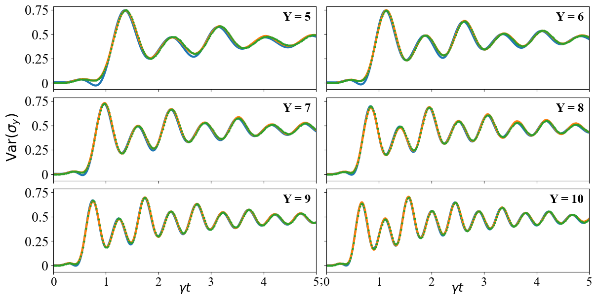
Figure S.2: Comparison of ${\rm Var}(\sigma_{y})$ plotted against the dimensionless time $\gamma t$ for the ideal case $\overline{n}=0$ and $\eta=1$, with three different methods and for six different driving strengths $Y$, indicated in the top-right corner of each panel. The Monte-Carlo average over $10^{4}$ realizations is plotted in orange. The blue line and green dots correspond to the analytical results obtained from the Dyson-series expansion to first order in $\gamma/\Omega$, and the moment-based equations, respectively. As the driving strength increases, so does the agreement between the three methods. Note the negative artefact in the short-time evolution of ${\rm Var}(\sigma_{y})$, which disappears when higher-order terms in $\gamma^{2}/\Omega^{2}$ are considered in Eq. (S.12). We also remark that in the long-time limit and for $Y\gg 1$, ${\rm Var}(\sigma_{y})+{\rm Var}(\sigma_{z})=\frac{1}{2}+\frac{1}{2}=1$. As in Fig. 2 of the main text, the atom is initialized to its ground state.

.5 Direct photoelectron-counting with imperfect detectors and/or a thermal bath

For a limited detector efficiency $\eta<1$ we cannot use a pure state to describe the evolution between collapses. Instead, the general form must be implemented in density matrix form. Between collapses the propagation rule reads

$$\ell^{\prime}\rho_{c}=(\mathcal{L}-\eta J)\rho_{c}=\frac{1}{i\hbar}[H,\rho_{c}]+\gamma(1-\eta)\sigma_{-}\rho_{c}\sigma_{+}-\frac{\gamma}{2}\{\rho_{c},\sigma_{+}\sigma_{-}\},$$ (S.34)

($\{.,.\}$ stands for the anti-commutator) while the collapse probability for the interval $(t,t+\Delta t]$ is

$$p_{c}(t)=\eta{\rm tr}[J\rho_{c}(t)]\Delta t=\eta(\gamma\Delta t){\rm tr}[\rho_{c}(t)\sigma_{+}\sigma_{-}],$$ (S.35)

and the (un-normalized) state becomes $\eta J\rho_{c}$. For $\eta\ll 1$, a single trajectory closely follows the deterministic evolution governed by the ME. This explains the significant reduction in the variance (the case for very weak drive), which – as we have seen in the main text – “responds” to quantum jumps and the oscillatory regression of the fluctuation.

If we now admit a thermal light injecting a photon flux $\gamma\overline{n}$, then the following term is added to the coherent evolution between collapses [to RHS of Eq. (S.34)]:

$$\gamma\overline{n}(\sigma_{-}\rho_{c}\sigma_{+}+\sigma_{+}\rho_{c}\sigma_{-}-\sigma_{+}\sigma_{-}\rho_{c}-\rho_{c}\sigma_{-}\sigma_{+}).$$ (S.36)

In the ideal case, $\overline{n}=0,\,\eta=1$, the series of photon “clicks” fully defines the quantum trajectory, since the wavefunction evolves under the action of $H_{\rm eff}$ defined in Eq. (S.3), being reset to the ground state after a spontaneous emission occurs. At optical frequencies, one has $\overline{n}\ll 1$, whence the most detrimental factor to the coherence of individual realizations is the limited detector efficiency. In that case, the propagation rule of Eq. (S.34) must be used between jumps which, for $\eta\ \ll 1$, coincides with the action of the Lindblad superoperator $\mathcal{L}$. Photoelectron counting and waiting-time distributions for nonunit detection efficiency are presented in Carmichael et al. (1989).

.6 Homodyne detection and quadrature amplitude squeezing

Let us briefly discuss a third type of unravelling (one of Wiener type), in addition to direct photodetection and heterodyne detection, the latter being equivalent to the quantum-state diffusion model Gisin and Percival (1992). In 1981, Walls and Zoller Walls and Zoller (1981) reported that light scattered in resonance fluorescence is squeezed in the field quadrature that is in phase with the mean scattered field amplitude, proportional to $\braket{\sigma_{-}}_{\rm ss}=+iY/(1+Y^{2})$ in the steady state, whence in a direction along $\theta=\pi/2$. A year later, Mandel came up with a scheme for detecting squeezing, which involved homodyning the scattered light with a strong local oscillator and measuring photon counting statistics as a function of the local oscillator phase Mandel (1982). Following this approach, the (un-normalized) conditional wavefunction evolves according to the stochastic Schrödinger equation

$$\frac{d}{dt}\ket{\overline{\psi}_{c}}=\frac{1}{i\hbar}H_{W}(t)\ket{\overline{\psi}_{c}},$$ (S.37)

in which $H_{W}(t)$ is the stochastic non-Hermitian Hamiltonian:

$$H_{W}(t)=H-i\hbar\gamma\sigma_{+}\sigma_{-}+i\hbar[\sqrt{\gamma}\braket{\psi_{c}(t)}{(e^{i\theta}\sigma_{+}+e^{-i\theta}\sigma_{-})}{\psi_{c}(t)}+\eta_{W}(t)]e^{-i\theta}\sqrt{\gamma}\sigma_{-},$$ (S.38)

where $\theta$ is the local-oscillator phase, $\ket{\psi_{c}(t)}$ is the normalized state and $\eta_{W}$ is a Gaussian white noise. Instances of the conditional variance ${\rm Var}(\sigma_{z})$ under this unravelling are depicted in Fig. 2 of the main text for $\theta=\pi/2$ and $\theta=0$. For an imperfect detector, the noise $\eta_{W}$ is replaced by two uncorrelated noise sources added in the proportion $\eta$ and $1-\eta$, with the former featuring in the photocurrent while the latter not Carmichael (1993). In Fig. 2 of the main text (bottom panels) we show that the QTAV ${\rm Var}(\sigma_{z})$ captures the redistribution of fluctuations among the squeezed and anti-squeezed quadratures. Finally, we recall that in heterodyne detection, $\theta$ is effectively replaced by $-(\omega_{LO}-\omega_{A})t$ (see Fig. 1 of the main text). The frequency mismatch between the local oscillator and the drive (here resonant with the atom) is assumed to be very large in comparison to the field fluctuations ($\sim\gamma$). A time average over the period $2\pi/(\omega_{LO}-\omega_{A})$ is then performed to simplify the resulting stochastic Schrödinger equation.

.7 Experimental setup and considerations

In this section, we describe the different experimental imperfections that can affect the measurements of a linear average of $\sigma_{z}$: the second-order correlation $g^{(2)}(\tau)$. The same spirit could be applied for non-linear averages. Second-order correlation functions are routinely measured experimentally using photon counting techniques in a Hanbury Brown and Twiss configuration. The photon flux enters a beam-splitter and both outputs are monitored by two detectors after a long integration time.

We consider real experimental data based on the setup of Bruno et al. (2019) in order to highlight the different imperfections. The experimental setup consists of a Maltese-cross coupling of single neutral atoms of ⁸⁷Rb. The atom is illuminated by a laser field with Rabi frequency $\Omega$ and detuning $\Delta$. The photons are collected by high-numerical aperture lenses, as shown in the main text, and the photon arrival times are measured [Fig. S.3(a)] using single-photon avalanche photodiodes (APDs). From these measurements, the normalized second-order correlation function between the lenses L1 and L2 is computed [Fig. S.3(b)]. The average atomic scattering rate on a single detector is $R_{\text{sca,det}}=9000$ counts/s.

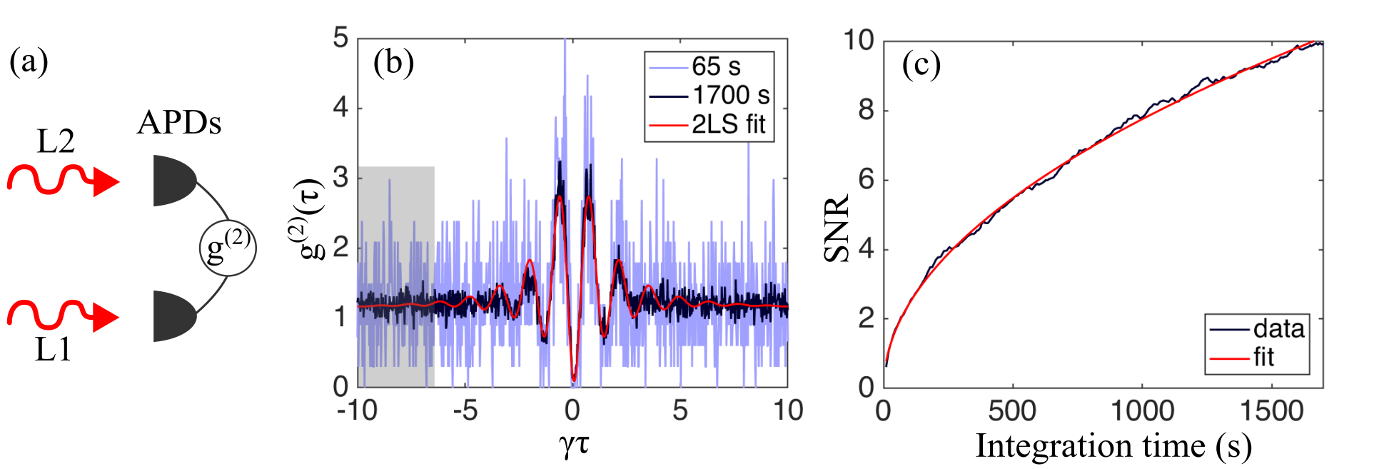
Figure S.3: (a) The arrival times of the photons coming from the lenses L1 and L2 are measured by avalanche photodiodes (APDs). (b) Normalized second-order correlation function for integration times of 65 (blue) or 1700 (black) seconds and fit using Eq. (S.39) from a two-level system approximation including experimental imperfections (red). The gray shaded box corresponds to the time range where the signal-to noise of $g^{(2)}$ is computed and shown in (c) as a function of the integration time and fitted by Eq. (S.40).

Let us focus on the measured correlation $g^{(2)}_{\text{mes}}(\tau)$ after a long integration time. The fit function for the correlation based on a two-level atom model and including different experimental imperfections is given by:

$$g^{(2)}_{\text{mes}}(\tau)=\frac{A(\tau)g^{(2)}(\tau,\Delta,\Omega)+\frac{2}{{\rm SNR}_{\text{Det}}}+\frac{1}{{\rm SNR}_{\text{Det}}^{2}}}{1+\frac{2}{{\rm SNR}_{\text{Det}}}+\frac{1}{{\rm SNR}_{\text{Det}}^{2}}},$$ (S.39)

where ${\rm SNR}_{\text{Det}}=R_{\text{sca,det}}/R_{\text{DC}}=18$ accounts for false positive photon detections due to the dark counts of the detectors. In the experiment, the dark count rate was $R_{\text{DC}}=500$ counts/s for each detector. Then, for single atoms, the photon counts are usually measured using red-detuned light in order to maintain the atom in the trap while acquiring the resonance fluorescence signal. A large negative detuning $\Delta<0$ causes an overshoot of the maximum value of $g^{(2)}$ above $2$. It is taken into account by an explicit dependence on the detuning of $g^{(2)}(\tau,\Delta,\Omega)$ which comes from the steady-state solution of the optical Bloch equations for a two-level atom. Finally, an empirical global envelop $A(\tau)=a+be^{-c\tau}$ takes into account the effect of the atomic motion in the trap Weber et al. (2006) where the parameters $a,b,c$ are extracted from a fit on microsecond timescales. After including these corrections, the correlation function is fitted from which we extract the Rabi frequency $\Omega=3.3\gamma$ and the detuning $\Delta=-3.2\gamma$. As shown on Fig. S.3(c), modeling the atom as a two-level system including experimental imperfections is enough to explain the experimental data. This agreement justifies the use of a two-level atom model to compute the different unravelings.

Now, let us consider that each photon flux arriving on the two detectors is measured with same efficiency $\eta$. In an optical detection system, $\eta$ is given by the product of the collection efficiency $\eta_{\text{col}}$, the optical path losses $\eta_{\text{loss}}$ and the quantum efficiency of the detectors $\eta_{\text{QE}}$. The $g^{(2)}$ statistics is recovered by measuring coincidences on two detectors over a large dataset after a long integration time $t_{\text{int}}$. In the long time limit ($\gamma\tau\gg 1$), where the counts are uncorrelated, the coincidences follow a Poissonian statistics. Therefore, the signal-to-noise ${\rm SNR}$ of the measured $g^{(2)}$ scales as:

$${\rm SNR}=\sqrt{\eta^{2}g^{(2)}R_{\text{sca,det}}t_{\text{int}}}.$$ (S.40)

Experimentally, we evaluate the signal-to-noise of the measured $g^{(2)}_{mes}$ [Fig. S.3(c)] by computing the ratio of the average and the standard deviation in the steady-state limit [gray shaded area in Fig. S.3(b)].

By fitting the signal-to-noise using Eq. (S.40), we end up with $\eta=0.25\%$. First, the optical losses $\eta_{\text{loss}}=50\%$ can be improved by a better mode-matching of the emitting spatial modes and the collecting optical fibers. Second, the detector quantum efficiency $\eta_{\text{QE}}=50\%$ at a specific wavelength $\lambda=780$ nm can be increased up to $90\%$ using superconducting nanowires Natarajan et al. (2012). Finally, for an atom scattering photons isotropically, the collection efficiency $\eta_{\text{col}}$ is determined by the solid angle covered by the optical system. Based on these numbers, we deduce the experimental collection efficiency of a single lens of $1\%$. By summing all channels up, the Maltese-cross coupling scheme employing the four lenses increases in principle this coupling by a factor of 4 for an atom tightly trapped in all spatial directions. Other geometries could also be used to increase the collection efficiency, such as a parabolic mirror trap Chou et al. (2017).