$T\bar{T}$ deformation on non-Hermitian two coupled SYK model

Abstract

We investigate $T\bar{T}$ deformation on non-Hermitian coupled Sachdev-Ye-Kitaev (SYK) model and the holographic picture. The relationship between ground state and thermofield double state is preserved under the $T\bar{T}$ deformation. We prove that $T\bar{T}$ deformed theory provides a reparameterization in large $N$ limit. These deformation effects is calculated numerically with green functions and free energy. The thermodynamic phase structures show the equivalence of the wormhole-black hole picture between non-Hermitian model and Hermitian model still holds under $T\bar{T}$ deformation. We also study the correlation function in Lorentz time and revival dynamic.

I.Introduction

SYK model consists of Majorana fermions with Guassian random coupling[1, 2, 3, 4]. It could be solve numerically in large $N$ limit. In low energy limit, the model emergent conformal symmetry with approximate SL(2,R)[5] which is dual to Nearly-AdS(NAdS) black hole and wormhole. The maximal Lyapunov exponents are now relate to a near horizon of black hole. An eternal traversable wormhole constructed by Maldacena an Qi gain increasing attention[6]. The duality is identical to two coupled SYK model. In previous work[7], we add a non-Hermitian bootstrap into original coupled SYK system. Our results show the non-Hermitian two coupled SYK model can provide thermodynamic structure equivalent to a Hermitian two coupled model. In this non-Hermitian two coupled SYK model, there is also a first-order phase transition from the low temperature traversable wormhole phase to the high temperature two black hole phase, which consists to the real time dynamics. The $T\bar{T}$ deformation on original un-coupled SYK₄ and SYK₂ model has been studied [8, 9]. $T\bar{T}$ deformation effectively couples the two local SYK₄ systems.

$T\bar{T}$ deformation[10, 11, 12] is an irrelevant deformation from IR to UV, with well-defined IR behaviours and a controllable UV limit. According to the divergence caused by deformations from IR to UV limit, deformations could be divided into different categories, relevant, marginal and irrelevant deformation. The $T\bar{T}$ deformation does not affect the divergent behaviours of UV. So it has an controllable property without affecting the UV constraint. In particular, we generally require the deformation coefficient $\lambda$ to be positive, but it can also be taken in the negative range. In two-dimensional theory, we can construct a composite operator $T\bar{T}$ via its energy-momentum tensor, and further obtain the Laplace relation $L(\lambda)$ with an additional deformation parameter $\lambda$. A deformation theory is defined and tricked by $T\bar{T}$ operator and its flow equation.

$$\frac{d\mathcal{L}^{\lambda}}{d\lambda}=\frac{1}{2}\epsilon^{\mu\upsilon}\epsilon^{mn}T_{\mu\nu}^{\lambda}T_{mn}^{\lambda}$$

We extend $T\bar{T}$ deformation to one dimensional theory while $T\bar{T}$ flow equations are diagonalized to 1d energy scalar[9]. This property provide an application to $T\bar{T}$ deformed AdS/CFT[13]. Since the $T\bar{T}$ operators is well defined, the entire deformation theory is captured in holography duality[14]. It could be employed on both quantum system and gravity side without breaking the holography duality. And some additional physical quantities can be solved in deformed conformal theory, such as the S-matrix, energy spectrum, correlation function, and entanglement entropy[15, 16, 17]. The $T\bar{T}$ deformed conformal field can be still described by holographic duality theory. For example, the duality of the Dirichlet boundary conditions can be applied to the finite radius of the AdS space boundary [18]. And a breaking of conformal symmetry is considered in holographic entanglement entropy, holographic complexity [19, 20].

Since $T\bar{T}$ deformation is relate to a non-local flow equation[21], the deformed theory with non-local terms is similar to effective bosonic string theory[22]. And we will show that the 1d $T\bar{T}$ deformation behaves like a effective bosonic string theory with the same Nambu-Goto action in this paper. Non-local effect induces correlation between different quantum systems. For example, we can also define an additional wormhole in $T\bar{T}$ deformed weakly relevant system, or enhance wormhole in strong coupling case. By definition, we have $T\bar{T}$ deformation would conserve charge like super symmetry[23], and classical integrable theory still remain integrability. For physical charges which is commute with Hamiltonian, it would be easily generate that the commutation with f(H). $T\bar{T}$ deformation also preserve integrability[24, 25]. Since the initiating operator $T\bar{T}$ is a dynamic tensor conserved flow which is constructed by a bilinear combination of flow equation, therefore these deformations also preserve the integrability of undeformed theory. $T\bar{T}$ operator is also a universal well defined operator in both IR and UV, therefore it would not cause any additional divergent correlation terms. The original integrability and holography[26, 27, 28] stay manifest under deformation. Moreover, the $T\bar{T}$ deformation on AdS/CFT could also be explained in several perspectives[29, 30, 31].

The main goal in this paper is to investigate whether the wormhole-black hole picture is robust not only in a Hermitian two coupled SYK model, but also in a non-Hermitian two coupled SYK model under $T\bar{T}$ deformation.

In section 2, we propose the $T\bar{T}$ deformed coupled SYK models in Hermitian and non-Hermitian case. In section 3, we start with the ground state of coupled SYK model. Then we match the overlap between the corresponding TFD and interaction model to evaluate the transmission property of wormhole before or after $T\bar{T}$ deformation. In section 4, we preform a $T\bar{T}$ deformation on NAdS spacetime and its reparameterized Schwarzian action to investigate the effects of $T\bar{T}$ deformation on holography. In section 5, we obtain the effective solution for large $N$ limit action. Then we evaluate the green function and thermal phase structure. In section 6, we study revival dynamic of coupled cSYK model. A numerical approximate correlation function in Lorentz time of black hole and wormhole situation have been obtained.

II.The model

We consider a coupled SYK model with interaction Hamiltonian

$$H=H_{L}+H_{R}+H_{int},$$ (1)

where $H_{L}$ and $H_{L}$ refers to the Hamiltonian of single side SYK model with Majorana fermions $\left\{\psi_{i},\psi_{j}\right\}=2\delta_{ij}$. The single side SYK model also turns to an additional complex bootstrap and conserve charge $\kappa$

$$H_{L}=H_{R}=\left(i\right)^{q/2}\sum_{1\leqslant j_{1}\leqslant j_{2}\cdots\ll j_{q}}^{N}{J_{j_{1}j_{2}\cdots j_{q}}\psi^{j_{1}}\psi^{j_{2}}\cdots\psi^{j_{q}}}-\kappa\sum_{i}{\psi^{i}\psi^{i}}.$$ (2)

Coupling matrix $J$ has independent Gaussian random

$$\left<J_{j_{1}\cdots j_{q}}\right>=0,$$

$$\left<J_{j_{1}\cdots j_{q}}^{2}\right>=\frac{2^{q-1}\mathcal{J}^{2}\left(q-1\right)!}{qN^{q-1}}.$$ (3)

We can also consider an additional interaction terms between left and right model

$$H_{int}=i\mu\sum_{j}{\psi_{L}^{j}}\psi_{R}^{j},$$ (4)

with operators reformism are written as

$$\psi_{A}^{2i-1}=e^{-\left(\delta_{AL}-\delta_{AR}\right)\alpha}C_{A}^{i\dagger}+e^{\left(\delta_{AL}-\delta_{AR}\right)\alpha}C_{A}^{i},$$

$$i\psi_{A}^{2i}=e^{-\left(\delta_{AL}-\delta_{AR}\right)\alpha}C_{A}^{i\dagger}-e^{\left(\delta_{AL}-\delta_{AR}\right)\alpha}C_{A}^{i}.$$ (5)

We can ignore the $\psi_{A}^{2i}$ terms in large $N$ limit for simplicity, and the interaction terms with complex actually have an additional U(1) term

$$H_{int}=i\mu\sum_{j}{\left(e^{i\phi}C_{L}^{j\dagger}C_{R}^{j}-e^{-i\phi}C_{R}^{j\dagger}C_{L}^{j}\right)}.$$ (6)

If we turn this U(1) freedom $\phi$ into the real, the corresponding interaction terms are Non-Hermitian

$$H_{int}=i\mu\sum_{j}{\left(e^{-2\alpha}C_{L}^{j\dagger}C_{R}^{j}-e^{2\alpha}C_{R}^{j\dagger}C_{L}^{j}\right)}.$$ (7)

The total $q=4$ Hamiltonian is

$$\begin{split}H&=-\sum_{ijkl}{J_{ijkl}}\left(2C_{i}^{L\dagger}C_{j}^{L\dagger}C_{k}^{L}C_{l}^{L}+2C_{i}^{R\dagger}C_{j}^{R\dagger}C_{k}^{R}C_{l}^{R}+4C_{i}^{L}C_{j}^{L\dagger}C_{k}^{L\dagger}C_{l}^{L}+4C_{i}^{R}C_{j}^{R\dagger}C_{k}^{R\dagger}C_{l}^{R}\right)\\ &+\sum_{i}{\left(-\kappa C_{i}^{L\dagger}C_{i}^{L}-\kappa C_{i}^{R\dagger}C_{i}^{R}+i\mu e^{-2\alpha}C_{i}^{L\dagger}C_{i}^{R}-i\mu e^{2\alpha}C_{i}^{R\dagger}C_{i}^{L}\right)}.\end{split}$$ (8)

Since $T\bar{T}$ deformation is triggered by 2d energy-momentum tensor. We can consider a $T\bar{T}$ operator by energy-momentum tensor

$$\mathcal{L}^{\left(\lambda+\delta\lambda\right)}=\mathcal{L}^{\left(\lambda\right)}-\delta\lambda T\bar{T}^{\left(\lambda\right)},$$

$$\frac{d\mathcal{L}^{\left(\lambda\right)}}{d\lambda}=\det T_{\mu\nu}^{\left(\lambda\right)}.$$ (9)

Moreover, $T\bar{T}$ deformation is still well defined in 1d theory, since the tensor operator and flow equation are diagonalized by

$$\frac{\partial S}{\partial\lambda}=\int{d\tau}\frac{T^{2}}{1/2-2\lambda T}.$$ (10)

This equation could be solved in a simple Nambu-Goto form[10]

$$H\left(\lambda\right)=f\left(H_{0},\lambda\right)=\frac{1}{4\lambda}\left(1-\sqrt{1-8\lambda\left(H_{0}-E_{0}\right)}\right),$$

$$L_{E}\left(H_{0},\lambda\right)=\psi_{i}\partial_{\tau}\psi_{i}+\frac{1}{4\lambda}\left(1-\sqrt{1-8\lambda\left(H_{0}-E_{0}\right)}\right).$$ (11)

In thermodynamics, $T\bar{T}$ deformation equal to a shifting on Hamiltonian with non-local effect. Parameter $E_{0}$ is an arbitrary constant mathematically, which could be determined by a physical fix point. And we will see that parameter $E_{0}$ could be set as 0 in large $N$ effective action in section 5.

To employ the disordering of Nambu-Goto action, we can apply a trick to linearize the Hamiltonians by introducing auxiliary field $\zeta$

$$S_{E}\left(H_{0},\lambda,\zeta\right)=\int{d\tau\left(\frac{1}{2}\psi_{i}\partial_{\tau}\psi_{i}-\frac{\zeta}{8\lambda}\left(1-\zeta^{-1}\right)^{2}+\zeta H_{0}-\zeta E_{0}\right)}.$$ (12)

Note that the averaged theory of q point interaction SYK model can obtained by dimensional analyse. $T\bar{T}$ deformation in SYK model can be written as

$$S_{E}\left(\lambda,\zeta\right)=\int{d\tau\left(\psi_{i}\partial_{\tau}\psi_{i}-\frac{\zeta}{8\lambda}\left(1-\zeta^{-1}\right)^{2}-\zeta E_{0}\right)}-\frac{N}{2q}\int{d\tau d\tau^{\prime}J^{2}}\zeta\left(\tau\right)\zeta\left(\tau^{\prime}\right)G^{q}\left(\tau,\tau^{\prime}\right).$$ (13)

From the effective action, the deformed Schwinger-Dyson equations has the same form to the undeformed one with $J^{2}$ rescaled by $J^{2}\zeta\left(\tau\right)\zeta\left(\tau^{\prime}\right)$. And the dimension analyse of the auxiliary field $\zeta$ shows that it exactly behaves equal to the coupling constant $J$. We need to find the $\zeta$ equation of motion

$$\frac{\zeta^{-2}-1}{8\lambda}-\frac{J^{2}}{q}\int{d\tau}\zeta\left(\tau\right)G^{q}\left(\tau,\tau^{\prime}\right)-\frac{E_{0}}{N}=0.$$ (14)

Since the $T\bar{T}$ deformation preserves the time translation invariant, the auxiliary field $\zeta\left(\tau\right)$ as the Lagrange multiplier should be a constant. Therefore we can find the $\zeta$ motion solution is

$$\zeta^{-1}=\sqrt{1+8\lambda\left(\frac{E_{0}}{N}+\frac{cJ}{q}\right)},$$ (15)

where c is a constant. And we find c is proportional to the integral of $G^{q}\left(\tau,\tau^{\prime}\right)$ by dimensional analysis.

III.Thermofield double state

Thermofield double(TFD) state successfully represent some indispensable structures of quantum wormhole. It enable a information transformation ability between two identical SYK model.

The ground states with a non-Hermitian bootstrap on interaction term are proposed as

$$\left|G\right>=\prod_{i=1}^{N}{\frac{1}{\sqrt{1+e^{4\alpha}}}}\left(\left|1\right>_{1,i}\left|0\right>_{2,i}\pm ie^{2\alpha}\left|0\right>_{1,i}\left|1\right>_{2,i}\right),$$ (16)

by utilizing $H_{int}\left|G\right>=\mu N\left|G\right>$. Here we perform a trace to non-Hermitian ground states and the corresponding density matrix[7, 39] $\rho_{A}=tr_{B}\left(\rho_{AB}\right)=tr_{B}\left(\left|G\right>\left<G\right|\right)$, which gives the diagonalized eigenvalues $\lambda_{1}=\frac{e^{4\alpha}}{1+e^{4\alpha}}$ and $\lambda_{2}=\frac{1}{1+e^{4\alpha}}$.

Notice that the degree of entanglement $E\left(\left|G\right>\right)=-\lambda_{1}\log_{2}\lambda_{1}-\lambda_{2}\log_{2}\lambda_{2}$ is equal to 1 and maximally entangled in Hermitian Hilbert space. However, this property have been broken since we introduce non-Hermitian constant.

$T\bar{T}$ deformation could be exactly represented by its chaotic behaviours. According to statistic definition of $T\bar{T}$ operator, energy-momentum flow should convergent to 0 without vertical excitation in low temperature limit. And Hamiltonian could also be approximatively represented by 0 statically. The $T\bar{T}$ deformation could be equally transformed into a constant shift of ground state energy for the additional arbitrary parameter in Nambu-Goto solution. For simplicity this constant can be set to 0 without breaking any physical observation. And it means an arbitrary deformation fix point has been moved into low temperature limit.

Since the thermal deformation could be represented by mapping the Hamiltonian in a certain way, the $T\bar{T}$ deformed thermofield double states are also evolving from the undeformed one

$$\left|TFD_{\lambda}\left(\beta\right)\right>=\exp\left(-\beta f\left(H,\lambda\right)/2\right)\left|I\right>.$$ (17)

Note that the definition of TFD state is irrelevant to coupling part, TFD $T\bar{T}$ deformation should be preformed independently. And it is nature to compare the deformed TFD to the deformation of MQ model which contains entangled models and its interaction parts.

SYK TFD state is a special quantum algebra system, which is relate to thermal structure and Hamiltonian in left and right copy Hilbert space.

$$\left|TFD_{0}\left(0\right)\right>=\frac{1}{2^{N/2}}\sum_{q}{\sum_{n_{q}}{\left|n_{q}\right>_{1}\otimes}}\left(e^{\frac{-i\eta\pi\varGamma}{4}}e^{iq\left(\frac{\pi}{2}\right)}\right)P\left|n_{q}\right>_{2},$$ (18)

where the left and right conjugate Hilbert space in TFD should satisfy fermion parity condition, and original TFD₀ state is maximally entangled

$$\varGamma=\left(-1\right)^{q+\frac{N}{2}},$$

$$P^{-1}C_{i}P=\eta P_{i}^{\dagger}.$$ (19)

Operator $P$ is introduced to represent the left and right parity conjugate, which brings a special fermion symmetry in TFD Hilbert space. $\phi$ is an additional arbitrary phase-evolving degree of freedom between two SYK models which is relate to the conserve charge of cSYK model.

Overlap between the ground states and thermofield double has an important role in exploring entanglement property and transformation between two coupled model. And the overlap remark credibility of the given holography theory dual to be a traversable wormhole.

When we set coupling $\mu$ close to infinite, equations in strong coupling limit are obtained. Left or right SYK Hamiltonian have been ignored and deformed Hamiltonian of entire system turns out to be

$$f\left(H\right)=f\left(H_{int}\right).$$ (20)

Diagonal element of TFD${}_{\beta}=0$ has been introduced in undeformed system

$$\begin{split}\left<TFD_{\beta=0}\right|H_{int}\left|TFD_{\beta=0}\right>&=\frac{1}{2^{N}}\sum_{qq^{\prime}}{\sum_{mn}{\left<\bar{n}_{-q^{\prime}}\right|_{2}\otimes\left<n_{q^{\prime}}\right|_{1}\left(i\mu\sum_{i}{\left(e^{-2\alpha}C_{i}^{L\dagger}C_{i}^{R}-e^{2\alpha}C_{i}^{R\dagger}C_{i}^{L}\right)}\right)}}\left|m_{q}\right>_{1}\otimes\left|\bar{m}_{-q}\right>_{2}\\ &=\frac{1}{2^{N}}\sum_{qq^{\prime}}{\sum_{nm}{\sum_{i}{\left(i\mu\right.}}}e^{i\pi\left(q+\frac{N}{2}\right)}e^{-2\alpha}\left<n_{q^{\prime}}\right|C_{i}^{L\dagger}\left|m_{q}\right>\left<\bar{n}_{-q^{\prime}}\right|C_{i}^{R}\left|\bar{m}_{-q}\right>\\ &\left.-i\mu e^{i\pi\left(q^{\prime}+\frac{N}{2}\right)}e^{2\alpha}\left<\bar{n}_{-q^{\prime}}\right|C_{i}^{R\dagger}\left|\bar{m}_{-q}\right>\left<n_{q^{\prime}}\right|C_{i}^{L}\left|m_{q}\right>\right)\\ &=\sum_{qq^{\prime}}{\sum_{nm}{\sum_{i}{\left(i\mu e^{2\alpha}-i\mu e^{-2\alpha}\right)}}}e^{-i\phi}/2^{N}\left<n_{q^{\prime}}\right|C_{i}^{L\dagger}\left|m_{q}\right>\left<m_{q}\right|C_{i}^{L}\left|n_{q^{\prime}}\right>\\ &=-\mu\left(e^{-2\alpha}+e^{2\alpha}\right)/2^{N}\sum_{q}{\sum_{n}{\sum_{i}{\left<n_{q^{\prime}}\right|C_{i}^{L\dagger}C_{i}^{L}\left|n_{q}\right>}}}=-\frac{\mu N}{2}\left(e^{-2\alpha}+e^{2\alpha}\right).\end{split}$$ (21)

Here Hilbert matrix elements are generated by operators-represented Hamiltonian

$$\left<\bar{n}_{-q^{\prime}}\right|C_{i}^{R}\left|n_{q^{{}^{\prime\prime\prime}}}^{\prime}\right>=-e^{i\pi\left(q+\frac{N}{2}\right)}e^{-i\phi}\left<m_{q^{\prime}}\right|C_{i}^{L}\left|n_{q^{\prime}}\right>,$$

$$\left<\bar{n}_{-q^{\prime}}\right|C_{i}^{R\dagger}\left|n_{q^{{}^{\prime\prime\prime}}}^{\prime}\right>=-e^{i\pi\left(q^{\prime}+\frac{N}{2}\right)}e^{-i\phi}\left<m_{q^{\prime}}\right|C_{i}^{L\dagger}\left|n_{q^{\prime}}\right>.$$ (22)

It is nature to define the $T\bar{T}$ deformation has no influence on zero-temperature theory. Similarly, we involve the deformed disorder average in strong coupling limit. $T\bar{T}$ deformation could be computed by the mapping Hamiltonian with the deformed Nambu-Goto form (12)

$$\left<f\left(H\right)\right>=\left<f\left(H_{int}\right)\right>=f\left<H_{int}\right>.$$ (23)

Likewise, we can also use the same process in weak coupling limit by ignoring the interaction term, a reduced Hamiltonian is obtained as

$$f\left(H\right)=f\left(H_{L}+H_{R}\right).$$ (24)

Similar to strong coupling limit, a finite deformation seem to be less important when inverse temperature $\beta$ approaches infinite

$$\left|TFD_{\beta\rightarrow\infty}\right>=\left|0\right>_{1,i}\left|\bar{0}\right>_{2,i},$$

$$\left<TFD_{\beta\rightarrow\infty}\right|H\left|TFD_{\beta\rightarrow\infty}\right>=\left<\bar{0}\right|_{2,i}\left<0\right|_{1,i}\sum_{ijkl}{J_{ijkl}}\sum_{a=L,R}{c_{i}^{a\dagger}}c_{j}^{a\dagger}c_{k}^{a}c_{l}^{a}\left|0\right>_{1,i}\left|\bar{0}\right>_{2,i}.$$ (25)

Obviously, this result is independent from interaction coupling $\mu$ and TFD $\beta=\infty$ is SYK eigenstate.

However, this result on overlap is no longer fixed in a more general inverse temperature $\beta$ condition. Numerically, we obtain an approximate overlap result between a arbitrary parameter $\beta$ and the ground states with the best-fixing coupling constant $\mu$

$$\left<TFD_{\lambda}\left(\beta\right)\middle|G\right>.$$ (26)

According to [39] the overlap in general inverse temperature $\beta$ condition is close to 1

$$\left<TFD_{0}\left(\beta\right)\middle|G\right>\approx 1.$$ (27)

And we can consider the $T\bar{T}$ deformed overlap between deformed TFD state which is generated with thermal deformed copied Hamiltonian and its best-fixing invalid deformed ground states

$$\left<TFD_{\lambda}\left(\beta\right)\middle|G\right>=\left<TFD_{0}\left(\beta\right)\right|\frac{\sqrt{Z_{0}\left(\beta\right)}}{\sqrt{Z_{\lambda}\left(\beta\right)}}\exp\left(-\beta\left(H-f\left(H,\lambda\right)\right)/2\right)\left|G\right>.$$ (28)

Conventionally, The ground states in overlap calculation could be generated by a simple infinite evolving, while the Hamiltonian has been substituted by deformed one

$$\left|G\left(t\right)\right>=\exp\left(-\tau\left(H_{L}+H_{R}+H_{int}\right)\right)\left|G\right>.$$ (29)

Since the TFD states are irrelevant to the interaction $\mu$, we can simply choose another ground state with a different coupling $\mu$ to remove this effects without changing the numerical overlap result in [39].

$$\left<TFD_{\lambda}\left(\beta\right)\middle|G\right>=\left<TFD_{0}\left(\beta\right)\right|\frac{\sqrt{Z_{0}\left(\beta\right)}}{\sqrt{Z_{\lambda}\left(\beta\right)}}\exp\left(-\beta\left(H-f\left(H,\lambda\right)\right)/2-\tau\left(H_{L}+H_{R}+H_{int}\right)\right)\left|0\right>=\left<TFD_{0}\left(\beta\right)\middle|G^{\prime}\right>.$$ (30)

Because the overlap equations have two degree of freedoms. The evolution of TFD states includes a finite deformation function $f$ and decoupled SYK Hamiltonian $H$, while the ground states side includes the interaction coupling $\mu$. In principle, we can easily absorb TFD deformation by shifting parameter $\mu$ to keep numerical overlap results invariant. This means $\beta$ or coupling $\mu$ also shift into a maximal overlap with a better fixed parametric condition without changing physical effects. And we have proved the numerical overlap between evolving ground state and deformed TFD is exactly equal to the undeformed theory with different coupling without cause any additional divergence.

IV.Deformed $NAdS_{2}$ spacetime and holography

In this section, we will derive the TTbar deformation on $NAdS_{2}$ spacetime. It is nature to consider a 2d gravitational $T\bar{T}$ deformation in bulk theory[13]. However, it seems more convenient to process with 1d quadratic stress tensor.

We suppose $NAdS_{2}$ geometry with Einstein gravity, which could be described as JT gravity [32, 33].

$$\begin{split}S&=\frac{\phi_{0}^{{}^{\prime}}}{2}\left[\int{\sqrt{g}R}+2\int_{Bdy}{\sqrt{g^{0}}K}\right]+\frac{1}{2}\left[\int{\phi^{\prime}\sqrt{g}\left(R+2\right)+2\int_{Bdy}{\phi_{b}^{{}^{\prime}}\sqrt{g^{0}}K}}\right]+S_{matter}\\ &=\frac{1}{2}\left[\int{\sqrt{g}\left(\phi_{0}R+\phi\right)}+2\int_{Bdy}{\sqrt{g^{0}}\phi_{b}K}\right]+S_{matter},\end{split}$$ (31)

with a constraint on boundary dilatons [34, 35] $\phi_{Bdy}^{\prime}=\phi_{b}^{\prime}$. The first and second part in (38) denote gravitational action on NAdS spacetime with curvatures. The third term contains a possible additional matter field, and this terms can be ignored in undeformed SYK model. $T\bar{T}$ deformation in AdS have been well proved as a boundary cutoff in [36], and we can follow the technique[13] and expand into NAdS with additional boundary dilatons. For simplicity, we introduce a modification into dilaton terms with diagonal gauge metric

$$\phi_{0}\left(r\right)=r\phi_{r}\left(r\right),$$

$$ds^{2}=N^{2}\left(r\right)d\tau^{2}+\frac{dr^{2}}{N^{2}\left(r\right)}.$$ (32)

Here AdS metric element $N^{2}$ could be written as

$$N^{2}\left(r\right)=f\left(\phi_{0}\right)\left(1-\frac{2M}{\phi_{r}\left(r\right)f\left(\phi_{0}\right)}\right).$$ (33)

$f(\phi_{0})$ depend on variable coordinate $\phi_{r}$ and bulk integral of $\phi$, and M is a constant with dimension of mass. Function f written as

$$f\left(\phi_{0}\right)=\frac{2}{\phi_{r}^{2}}\int_{\phi_{0}}{\phi\left(x\right)dx}.$$ (34)

If we consider a finite Dirichlet radial cutoff, the quasilocal bulk energy solution is given by

$$E_{bulk}=\phi_{r}r_{c}\left(1-\frac{1}{r_{c}}\sqrt{f\left(\phi_{0}\left(r_{c}\right)\right)-2M/\phi_{r}}\right),$$ (35)

which is familiar with Nambu-Goto-like Hamiltonian. We may expect a $T\bar{T}$ deformation formalism. We now seek for a method to perform the $T\bar{T}$ deformation equation with

$$\frac{\partial S}{\partial\lambda}=\int{d\tau}\frac{T^{2}}{1/2-2\lambda T}.$$ (36)

In order to find the $T\bar{T}$ operator with energy-momentum flow, we can define a Brown-York stress scalar with renormalization. 2d $T\bar{T}$ flow is obtained by variation of metric $g^{0}$ and bulk EFT dilaton $\phi_{0}$. While the metric and stress tensor are passively transformed. We define

$$g_{\tau\tau}^{0}=r_{c}^{2}\gamma_{\tau\tau},$$

$$T^{\tau\tau}=r_{c}\tilde{T}^{\tau\tau}=\frac{2}{\sqrt{g^{0}}}\frac{\delta S}{\delta g^{0}},$$

$$O=r_{c}^{-2}\tilde{O}=\frac{1}{\sqrt{g^{0}}}\frac{\delta S}{\delta\phi_{0}}.$$ (37)

We can involve the boundary conditions of $NAdS_{2}$ into tensors without changing the equations. According to the definition of $T\bar{T}$ deformation, the $NAdS_{2}$ flow equation could be preformed with a similar $T\bar{T}$ operator.

The flow equation of effective action with on-shell Hamiltonian constraint

$$r_{c}\frac{\partial}{\partial r_{c}}S_{EFT}=\int{d\tau\sqrt{\gamma}\left(\frac{-\tilde{T}_{\tau}^{\tau}+\phi_{r}^{2}r_{c}^{4}+\phi_{r}r_{c}^{3}\phi\left(r_{c}\phi_{r}\right)}{\phi_{r}r_{c}^{2}-\tilde{T}_{\tau}^{\tau}}\right)}.$$ (38)

Notice that the flow equation now exactly has the same mathematical form with $T\bar{T}$ deformation. By comparing formulas we have mentioned, we obtain the deformation parameter $\lambda$ in $NAdS_{2}$ spacetime

$$\lambda=\frac{1}{4\phi_{r}r_{c}^{2}}.$$ (39)

Thus we can write the flow equation with boundary cut off in $T\bar{T}$ deformation form

$$\frac{\partial S_{EFT}}{\partial\lambda}=\int{d\tau\sqrt{\gamma}\left(\frac{T-\left(1+\left(r_{c}\phi_{r}\right)^{-1}\phi\left(r_{c}\phi_{r}\right)\right)/\left(16\lambda^{2}\right)}{1/2-2\lambda T}\right)}.$$ (40)

Here we set the diagonal $T\bar{T}$ stress tensor with

$$T=\tilde{T}_{\tau}^{\tau}.$$ (41)

The deformation equation could also be written with Hamiltonian

$$\frac{\partial E}{\partial\lambda}=\frac{E^{2}-\left(1+\frac{\sqrt{4\phi_{r}\lambda}}{\phi_{r}}\phi\left(\frac{\phi_{r}}{\sqrt{4\phi_{r}\lambda}}\right)\right)/\left(16\lambda^{2}\right)}{1/2-2\lambda E},$$ (42)

which may generate a simple Nambu-Goto solution

$$E\left(\lambda\right)=\frac{1}{4\lambda}\left(1-\sqrt{4\phi_{r}\lambda}f\left(\frac{\phi_{r}}{\sqrt{4\phi_{r}\lambda}}\right)-8\lambda E_{0}\right).$$ (43)

So we have proved that the $T\bar{T}$ deformation of $NAdS_{2}$ bulk metric exactly equal to a finite radial Dirichlet boundary cut off. However, this does not mean to abandon the geometry between deformed radial boundary and nature $NAdS_{2}$ boundary which becomes indistinguishable. We focus on the dynamic and energy-momentum flow on radial Dirichlet sphere which is exactly equal to the $T\bar{T}$ deformation. And we may find a similar flow equation as $T\bar{T}$ deformation in NAdS spacetime as dual coupled SYK does. The boundary interaction term is added in MQ model

$$S_{int}=h\sum_{i}{\int{duO_{L}^{i}\left(u\right)O_{R}^{i}\left(u\right)}}.$$ (44)

The semi-classical interaction operators $O$ is set with conformal dimension of $\Delta$. And the constant $h$ mark the stress with conformal limit. Since the interaction term is irrelevant to metric tensor $g$, this additional term does not break the physical effects of $T\bar{T}$ deformation.

The bulk theory reduce to Schwarzian form by a time reparametrization and lead to symmetry breaking. We would like to involve $T\bar{T}$ deformation to effective Schwarzian theory without breaking holography duality. We can introduce

$$S_{E}=-C\int{d\tau\left(Sch\left(h,\tau\right)+W\left(h^{\prime}\right)\right)},$$ (45)

where $C$ is a constant. And it can be defined as a dilaton reparametrization on boundary $\phi_{Bdy}^{\prime}=\phi_{b}^{\prime}=\frac{\bar{\phi}_{r}}{\epsilon}$ and $ds\left|{}_{Bdy}=\frac{d\tau}{\epsilon}\right.$ in eq.(31) Taking $\epsilon$ to infinitesimal, and we have

$$C=\bar{\phi}_{r}.$$ (46)

And in dual SYK effective theory, C also could be some quantum constants which depend on four point correlation function

$$C=N\alpha_{S}.$$ (47)

Function $W\left(h^{\prime}\right)$ is an arbitrarily function of $h^{\prime}$ , and determined by the specific action which is distinguish form pure Schwarzian derivative.

Taking $W\left(h^{\prime}\right)$ to zero, the theories reduce to pure Schwarzian derivative

$$Sch\left(h,\tau\right)=\left(\frac{h^{\prime\prime}}{h^{\prime}}\right)^{{}^{\prime}}-\frac{1}{2}\left(\frac{h^{\prime\prime}}{h^{\prime}}\right)^{2}.$$ (48)

One can consider time reparametrization of a radial cutoff metric, but it seems more convenient to deform Schwarzian action directly. We can also expand the technique of $T\bar{T}$ deformed Schwarzian action in [13] to effective action of MQ model. The first step toward $T\bar{T}$ deformation is to find the energy-momentum tensor and restore its flow equation, and we can pick a canonical coordinates with Ostrogradsky formalism[37]

$$q_{1}=h,$$

$$q_{2}=h^{\prime}=e^{\phi},$$ (49)

with canonical momentums

$$p_{1}=\frac{\partial L}{\partial h^{\prime}}-\frac{d}{d\tau}\left(\frac{\partial L}{\partial h^{\prime\prime}}\right)=C\left(\frac{h^{\prime\prime 2}}{h^{\prime 3}}-\frac{h^{\prime\prime\prime}}{h^{\prime 2}}-w\left(h^{\prime}\right)\right),$$

$$p_{2}=\frac{\partial L}{\partial h^{\prime\prime}}=C\frac{h^{\prime\prime}}{h^{\prime 2}}.$$ (50)

The Hamiltonian is invariant under coordinate transformation

$$H=\frac{p_{2}^{2}q_{2}^{2}}{2C}+\frac{C}{2}q_{2}^{2}+p_{1}q_{2}.$$ (51)

Note that the $T\bar{T}$ deformation could be projected via Hamiltonian form

$$H\left(\lambda\right)=\frac{1}{4\lambda}\left(1-\sqrt{1-8\lambda H_{0}}\right).$$ (52)

We obtain the deformed Lagrangian by Legendre transformation with rotation $\tau\rightarrow-i\tau$,$q_{2}\rightarrow iq_{2}$

$$L_{E}\left(\lambda\right)=-\frac{\left(h^{\prime}-e^{\phi}\right)}{8\lambda h^{\prime}e^{\phi}}+\frac{C}{2}\frac{e^{\phi}}{h^{\prime}}\left(\phi^{\prime 2}-h^{\prime}f\left(h^{\prime}\right)\right).$$ (53)

First we preform a deformation to low energy effective SYK theory, which has an SL(2) boundary reparameter symmetry and a pure Schwarzian derivatives without additional function $W\left(h^{\prime}\right)$

$$S=-C\int{du\left\{t_{P}\left(u\right),u\right\}},$$ (54)

we can apply a simple Lorentzian solution

$$S_{E}=-C\int{d\tau\left\{\tanh\frac{\mathrm{h}\left(\tau\right)}{2},\tau\right\}}.$$ (55)

Corresponding deformed Lagrangian are parametrized from boundary

$$L_{E}\left(\lambda\right)=-\frac{\left(\tanh\frac{\mathrm{h}\left(\tau\right)}{2}^{\prime}-e^{\phi}\right)}{8\lambda\tanh\frac{\mathrm{h}\left(\tau\right)}{2}^{\prime}e^{\phi}}+\frac{C}{2}\frac{e^{\phi}}{\tanh\frac{\mathrm{h}\left(\tau\right)}{2}^{\prime}}\left(\phi^{\prime 2}\right).$$ (56)

After involving constant C, we have the holography effective action

$$L_{E}\left(\lambda\right)=-\frac{\left(\tanh\frac{\mathrm{h}\left(\tau\right)}{2}^{\prime}-e^{\phi}\right)}{8\lambda\tanh\frac{\mathrm{h}\left(\tau\right)}{2}^{\prime}e^{\phi}}-\frac{\bar{\phi}_{r}}{2}\frac{e^{\phi}}{\tanh\frac{\mathrm{h}\left(\tau\right)}{2}^{\prime}}\left(\phi^{\prime 2}\right),$$ (57)

which can be written as

$$L_{E}\left(\lambda\right)=-\frac{\left(\tanh\frac{\mathrm{h}\left(\tau\right)}{2}^{\prime}-e^{\phi}\right)}{8\lambda\tanh\frac{\mathrm{h}\left(\tau\right)}{2}^{\prime}e^{\phi}}-\frac{N\alpha_{S}}{2}\frac{e^{\phi}}{\tanh\frac{\mathrm{h}\left(\tau\right)}{2}^{\prime}}\left(\phi^{\prime 2}\right).$$ (58)

The conformal transformation with additional complex U(1) symmetry is given [40, 41]

$$\tilde{G}_{AB}\left(\tau,\tau\prime\right)=\left[h_{A}^{\prime}\left(\tau\right)h_{B}^{\prime}\left(\tau^{\prime}\right)\right]^{\varDelta}G_{AB}\left(h\left(\tau\right),h\left(\tau^{\prime}\right)\right)e^{i\left(\varphi_{A}-\varphi_{B}\right)},$$

$$\tilde{\varSigma}_{AB}\left(\tau,\tau\prime\right)=\left[h_{A}^{\prime}\left(\tau\right)h_{B}^{\prime}\left(\tau^{\prime}\right)\right]^{1-\varDelta}G_{AB}\left(h\left(\tau\right),h\left(\tau^{\prime}\right)\right)e^{i\left(\varphi_{A}-\varphi_{B}\right)}.$$ (59)

Left and right copy Schwarzian action has an U(1) anomalous term terms to preserve transformation symmetry

$$S=-N\alpha_{S}\int{d\tau\left\{\tanh\frac{\mathrm{h}\left(\tau\right)}{2},\tau\right\}}+\frac{NK}{2}\int{d\tau\left(\varphi^{\prime}\left(\tau\right)+i\varepsilon h^{\prime}\left(\tau\right)\right)}^{2},$$ (60)

where $\varepsilon$ is a constant relates to U(1) generator $\varphi$. The general reparametrized Schwarzian action nearly performs SL(2,R)$\times$U(1) Virasoro-Kac-Moody symmetry. And we find corresponding function $w\left(h^{\prime}\right)$ in SL(2,R)$\times$U(1) Schwarzian theory

$$w\left(h^{\prime}\right)=\frac{i\varepsilon NK}{C}\left(\varphi^{\prime}\left(\tau\right)+i\varepsilon h^{\prime}\left(\tau\right)\right).$$ (61)

This result leads to the deformed Lagrangian

$$L_{E}\left(\lambda\right)=-\frac{\left(\tanh\frac{\mathrm{h}\left(\tau\right)}{2}^{\prime}-e^{\phi}\right)}{8\lambda\tanh\frac{\mathrm{h}\left(\tau\right)}{2}^{\prime}e^{\phi}}-\frac{N\alpha_{S}}{2}\frac{e^{\phi}}{\tanh\frac{\mathrm{h}\left(\tau\right)}{2}^{\prime}}\left(\phi^{\prime 2}-\tanh\frac{\mathrm{h}\left(\tau\right)}{2}^{\prime}\left(\frac{i\varepsilon K}{\alpha_{S}}\left(\varphi^{\prime}\left(\tau\right)+i\varepsilon h^{\prime}\left(\tau\right)\right)\right)\right),$$ (62)

and the coupled part of effective action between two SYK model is given as

$$S_{int}=\frac{\mu}{2}\int{d\tau\left[\frac{Bh_{L}^{{}^{\prime}}\left(\tau\right)h_{R}^{{}^{\prime}}\left(\tau\right)}{\cosh^{2}\left(\frac{h_{L}\left(\tau\right)-h_{R}\left(\tau\right)}{2}\right)}\right]}^{\varDelta}.$$ (63)

Since we $T\bar{T}$ deform the total action with decoupled models and its interaction, which is described by Schwarzian derivative and reparameterized interaction operators

$$S_{total}=2S+S_{int},$$ (64)

with non-Hermitian boundary interaction operators

$$S_{int}=g\sum_{i}{\int{du}(e^{-2\alpha}O_{L}^{i\dagger}(u)O_{R}^{i}(u)-e^{2\alpha}O_{R}^{i\dagger}(u)O_{L}^{i}(u))}.$$ (65)

The corresponding function $w$ become

$$w\left(h^{\prime}\right)=\frac{i\varepsilon K}{2\alpha_{S}}\left(\varphi^{\prime}\left(\tau\right)+i\varepsilon h^{\prime}\left(\tau\right)\right)+\frac{\varDelta B^{\varDelta}\mu}{\cosh^{2\varDelta}\left(\frac{h_{L}\left(\tau\right)-h_{R}\left(\tau\right)}{2}\right)}\left[h_{L}^{{}^{\prime}}\left(\tau\right)h_{R}^{{}^{\prime}}\left(\tau\right)\right]^{\varDelta-\frac{1}{2}},$$ (66)

and we obtain the corresponding Lagrangian

$$\begin{split}L_{E}\left(\lambda\right)&=-\frac{\left(\tanh^{\prime}\frac{\mathrm{h}\left(\tau\right)}{2}-e^{\phi}\right)}{8\lambda\tanh^{\prime}\frac{\mathrm{h}\left(\tau\right)}{2}e^{\phi}}-N\alpha_{S}\frac{e^{\phi}}{\tanh^{\prime}\frac{\mathrm{h}\left(\tau\right)}{2}}\\ &\times\left(\phi^{\prime 2}-\tanh^{\prime}\frac{\mathrm{h}\left(\tau\right)}{2}\left(\frac{i\varepsilon K}{2\alpha_{S}}\left(\varphi^{\prime}\left(\tau\right)+i\varepsilon h^{\prime}\left(\tau\right)\right)+\frac{\varDelta B^{\varDelta}\mu}{\cosh^{2\varDelta}\left(\frac{h_{L}\left(\tau\right)-h_{R}\left(\tau\right)}{2}\right)}\left[h_{L}^{{}^{\prime}}\left(\tau\right)h_{R}^{{}^{\prime}}\left(\tau\right)\right]^{\varDelta-\frac{1}{2}}\right)\right).\end{split}$$ (67)

We can also consider the additional U(1) parameter $\varphi$ and non-Hermitian parameter $\alpha$ into the interaction term

$$\begin{split}S_{int}&=\frac{\mu}{2}\int{d\tau\left[\frac{Bh_{L}^{{}^{\prime}}\left(\tau\right)h_{R}^{{}^{\prime}}\left(\tau\right)}{\cosh^{2}\left(\frac{h_{L}\left(\tau\right)-h_{R}\left(\tau\right)}{2}\right)}\right]}^{\varDelta}\cosh\left(\varepsilon h_{L}\left(\tau\right)-\varepsilon h_{R}\left(\tau\right)\right)\\ &\times\left[\exp\left(i\left(\varphi_{L}-\varphi_{R}\right)-2\alpha\right)+\exp\left(-i\left(\varphi_{L}-\varphi_{R}\right)+2\alpha\right)\right].\end{split}$$ (68)

For function w, this variation is equal to add a external structure

$$\begin{split}w\left(h^{\prime}\right)&=\frac{i\varepsilon K}{2\alpha_{S}}\left(\varphi^{\prime}\left(\tau\right)+i\varepsilon h^{\prime}\left(\tau\right)\right)+\frac{\varDelta B^{\varDelta}\mu}{\cosh^{2\varDelta}\left(\frac{h_{L}\left(\tau\right)-h_{R}\left(\tau\right)}{2}\right)}\left[h_{L}^{{}^{\prime}}\left(\tau\right)h_{R}^{{}^{\prime}}\left(\tau\right)\right]^{\varDelta-\frac{1}{2}}\\ &\times\left(\cosh\left(\varepsilon h_{L}\left(\tau\right)-\varepsilon h_{R}\left(\tau\right)\right)\times\left[\exp\left(i\left(\varphi_{L}-\varphi_{R}\right)-2\alpha\right)+\exp\left(-i\left(\varphi_{L}-\varphi_{R}\right)+2\alpha\right)\right]\right),\end{split}$$ (69)

corresponding Lagrangian also includes the external exponent

$$\begin{split}L_{E}\left(\lambda\right)&=-\frac{\left(\tanh^{\prime}\frac{\mathrm{h}\left(\tau\right)}{2}-e^{\phi}\right)}{8\lambda\tanh^{\prime}\frac{\mathrm{h}\left(\tau\right)}{2}e^{\phi}}-N\alpha_{S}\frac{e^{\phi}}{\tanh^{\prime}\frac{\mathrm{h}\left(\tau\right)}{2}}\\ &\times\left(\phi^{\prime 2}-\tanh^{\prime}\frac{\mathrm{h}\left(\tau\right)}{2}\left(\frac{i\varepsilon K}{2\alpha_{S}}\left(\varphi^{\prime}\left(\tau\right)+i\varepsilon h^{\prime}\left(\tau\right)\right)+\frac{\varDelta B^{\varDelta}\mu}{\cosh^{2\varDelta}\left(\frac{h_{L}\left(\tau\right)-h_{R}\left(\tau\right)}{2}\right)}\left[h_{L}^{{}^{\prime}}\left(\tau\right)h_{R}^{{}^{\prime}}\left(\tau\right)\right]^{\varDelta-\frac{1}{2}}\right)\right.\\ &\times\left.\left(\cosh\left(\varepsilon h_{L}\left(\tau\right)-\varepsilon h_{R}\left(\tau\right)\right)\times\left[\exp\left(i\left(\varphi_{L}-\varphi_{R}\right)-2\alpha\right)+\exp\left(-i\left(\varphi_{L}-\varphi_{R}\right)+2\alpha\right)\right]\right)\right).\end{split}$$ (70)

Now we switch to gravitational Schwarzian action with non-Hermitian boundary interaction, which lead to a renormalized effective action

$$\begin{split}S_{int}&=\frac{gN}{2^{2\varDelta}}\int{d\tau}\left[\frac{h_{L}^{{}^{\prime}}\left(\tau\right)h_{R}^{{}^{\prime}}\left(\tau\right)}{\cosh^{2}\left(\frac{h_{L}\left(\tau\right)-h_{R}\left(\tau\right)}{2}\right)}\right]^{\varDelta}\cosh\left(\varepsilon h_{L}\left(\tau\right)-\varepsilon h_{R}\left(\tau\right)\right)\\ &\times\left[\exp\left(i\left(\varphi_{L}-\varphi_{R}\right)-2\alpha\right)+\exp\left(-i\left(\varphi_{L}-\varphi_{R}\right)+2\alpha\right)\right].\end{split}$$ (71)

And gravitational Lagrangian is given as

$$\begin{split}L_{E}\left(\lambda\right)&=-\frac{\left(\tanh^{\prime}\frac{\mathrm{h}\left(\tau\right)}{2}-e^{\phi}\right)}{8\lambda\tanh^{\prime}\frac{\mathrm{h}\left(\tau\right)}{2}e^{\phi}}-\bar{\phi}_{r}\frac{e^{\phi}}{\tanh^{\prime}\frac{\mathrm{h}\left(\tau\right)}{2}}\\ &\times\left(\phi^{\prime 2}-\tanh^{\prime}\frac{\mathrm{h}\left(\tau\right)}{2}\left(\frac{i\varepsilon\tilde{K}}{2\bar{\phi}_{r}}\left(\varphi^{\prime}\left(\tau\right)+i\varepsilon h^{\prime}\left(\tau\right)\right)+\frac{gN\varDelta}{2^{2\varDelta-1}\cosh^{2\varDelta}\left(\frac{h_{L}\left(\tau\right)-h_{R}\left(\tau\right)}{2}\right)}\left[h_{L}^{{}^{\prime}}\left(\tau\right)h_{R}^{{}^{\prime}}\left(\tau\right)\right]^{\varDelta-\frac{1}{2}}\right)\right.\\ &\times\left.\left(\cosh\left(\varepsilon h_{L}\left(\tau\right)-\varepsilon h_{R}\left(\tau\right)\right)\times\left[\exp\left(i\left(\varphi_{L}-\varphi_{R}\right)-2\alpha\right)+\exp\left(-i\left(\varphi_{L}-\varphi_{R}\right)+2\alpha\right)\right]\right)\right),\end{split}$$ (72)

which has the same form as eq.(44)

The deformation is relevant to mathematical formalism $h$ and $h^{\prime}$, but $T\bar{T}$ deformation does not affect its physical coefficients, $T\bar{T}$ deformation on effective action would not break holography duality

$$\bar{\phi}_{r}=N\alpha_{S},$$

$$\frac{\mu B^{\varDelta}}{2}=\frac{gN}{2^{2\varDelta}}.$$ (73)

V.Thermal phase structure

In this section, we first consider un-coupled SYK model under the $T\bar{T}$ deformation. $T\bar{T}$ deformation in 1d quantum system like SYK has been well proposed[14]. And we will consider a two deformed cSYK model coupled with a chemical potential $\mu$. In deform expansion of partition function, We can introduce auxiliary fields $\zeta$ to represent the deformation of partition function. And in $T\bar{T}$ deformed SYK model[14, 8], the coupling constant $J$ is substituted by $J\zeta$. The difference is that the auxiliary field in coupled theory also contains the entanglement

$$-\frac{S_{E}}{N}=\log\det\left(\partial_{\tau}\delta_{AB}-\varSigma_{AB}\right)+\frac{1}{2}\int{d\tau d\tau^{\prime}}\sum_{AB}{\left[\varSigma_{AB}\left(\tau,\tau^{\prime}\right)G_{BA}\left(\tau^{\prime},\tau\right)-\frac{2^{2q-2}J^{2}}{q^{2}}G_{AB}^{q}\left(\tau,\tau^{\prime}\right)G_{BA}^{q}\left(\tau^{\prime},\tau\right)\right]}.$$ (74)

The action of two independence SYK theory and its coupling are linearized by disorder averaging. In order to obtain action in analytical form, we should also linearize the deformed theory to a similar form. We can employ a trick to transform the action form by introducing an auxiliary field $\zeta$. The action function is obtained

$$S_{E}\left(H_{0},\lambda,\zeta\right)=\int{d\tau\left(\frac{1}{2}\delta_{AB}\psi_{i}\partial_{\tau}\psi_{i}-\frac{\zeta}{8\lambda}\left(1-\zeta^{-1}\right)^{2}+\zeta H_{0}-\zeta E_{0}\right)},$$ (75)

with the constraint

$$H\left(\lambda\right)+H_{0}-E_{0}-2\lambda H\left(\lambda\right)^{2}=0.$$ (76)

The 1st order interaction term is involved in the deformation entropy and it could be written as the deformed formula. Since auxiliary field $\zeta$ is dimensionless, the $T\bar{T}$ deformed model in thermal limit behaves exactly like a shifting coupling constant $J$, so we can rescale the coupling constant $J$ as $J\zeta$. The large $N$ effective action reads

$$-\frac{S_{E}}{N}=\log\det\left(\partial_{\tau}\delta_{AB}-\varSigma_{AB}\right)+\frac{1}{2}\int{d\tau d\tau^{\prime}}\sum_{AB}{\left[\varSigma_{AB}\left(\tau,\tau^{\prime}\right)G_{BA}\left(\tau^{\prime},\tau\right)-\frac{2^{2q-2}J^{2}\zeta^{2}}{q^{2}}G_{AB}^{q}\left(\tau,\tau^{\prime}\right)G_{BA}^{q}\left(\tau^{\prime},\tau\right)\right]}.$$ (77)

We consider large $N$ effective action of the coupled SYK model with q point interaction and Hermitian interaction is lead to MQ model

$$-\frac{S_{E}}{N}=\log\det\left(\sigma_{AB}-\varSigma_{AB}\right)+\frac{1}{2}\int{d\tau d\tau\prime}\sum_{AB}{\left[\varSigma_{AB}\left(\tau,\tau\prime\right)G_{BA}\left(\tau\prime,\tau\right)-\frac{2^{2q-2}J^{2}}{q^{2}}G_{AB}^{q}\left(\tau,\tau\prime\right)G_{BA}^{q}\left(\tau\prime,\tau\right)\right]},$$ (78)

where

$$\sigma_{AB}=\left(\begin{matrix}\partial_{\tau}&i\mu\\ -i\mu&\partial_{\tau}\\ \end{matrix}\right).$$ (79)

The non-Hermitian interaction Hamiltonian term and conserved charge turn to be

$$H_{int}=\sum_{i}{\left(-i\mu e^{2\alpha}G_{LR,i}+i\mu e^{-2\alpha}G_{RL,i}-\kappa G_{LL,i}-\kappa G_{RR,i}\right)}.$$ (80)

Accordingly, we add a conserved charge and $\sigma_{AB}$ become

$$\sigma_{AB}=\left(\begin{matrix}\partial_{\tau}-\kappa&i\mu e^{-2\alpha}\\ -i\mu e^{2\alpha}&\partial_{\tau}-\kappa\\ \end{matrix}\right).$$ (81)

And non-Hermitian parameter $\alpha$ redefines the L-R and R-L coupling, Then the corresponding equations are now simplified to

$$G_{ab}\left(i\omega_{n},\alpha\right)=\frac{\left(-i\omega_{n}-\kappa\right)\delta_{ab}-\varSigma_{ba}\left(i\omega_{n},\alpha\right)-i\mu e^{-2\alpha}\delta_{aL}\delta_{bR}+i\mu e^{2\alpha}\delta_{aR}\delta_{bL}}{\left(-i\omega_{n}-\kappa-\varSigma_{LL}\right)\left(-i\omega_{n}-\kappa-\varSigma_{RR}\right)-\left(i\mu e^{-2\alpha}-\varSigma_{LR}\right)\left(-i\mu e^{2\alpha}-\varSigma_{RL}\right)},$$ (82)

with Matsubara frequency $\omega_{n}=2\pi\left(n+\frac{1}{2}\right)/\beta$. The symmetry $G_{LL}\left(i\omega_{n},\alpha\right)=G_{RR}\left(i\omega_{n},\alpha\right)$, $G_{LR}\left(i\omega_{n},\alpha\right)=-G_{RL}\left(i\omega_{n},-\alpha\right)$, $\varSigma_{LR}\left(i\omega_{n},\alpha\right)=-\varSigma_{RL}\left(i\omega_{n},-\alpha\right)$ preserve under $T\bar{T}$ deformation.

By solving the equation of motion of the auxiliary field $\zeta$, which is derived from the action of the Hermitian coupled SYK model under the $T\bar{T}$ deformation

$$\begin{split}S_{E}\left(\lambda,\zeta\right)&=\int{d\tau}\left(\psi_{i}\partial_{\tau}\psi_{i}-\frac{\zeta}{8\lambda}\left(1-\zeta^{-1}\right)^{2}-\zeta E_{0}\right)-\frac{2^{2q-2}J^{2}N}{q^{2}}\int{d\tau_{1}d\tau_{2}}\zeta^{2}G_{AB}^{q}\left(\tau_{1},\tau_{2}\right)G_{BA}^{q}\left(\tau_{2},\tau_{1}\right)\\ &+\frac{N}{2}\int{d\tau_{1}d\tau_{2}}\zeta^{2}\left(i\mu e^{2\alpha}G_{LR}\left(\tau_{1},\tau_{2}\right)\delta\left(\tau_{2}-\tau_{1}\right)-i\mu e^{-2\alpha}G_{RL}\left(\tau_{2},\tau_{1}\right)\delta\left(\tau_{1}-\tau_{2}\right)\right)\\ &-\frac{N}{2}\int{d\tau_{1}d\tau_{2}}\zeta^{2}\left(\kappa G_{LL}\left(\tau_{1},\tau_{2}\right)\delta\left(\tau_{2}-\tau_{1}\right)+\kappa G_{RR}\left(\tau_{1},\tau_{2}\right)\delta\left(\tau_{2}-\tau_{1}\right)\right).\end{split}$$ (83)

where $\zeta$ is solute by

$$\begin{split}\zeta^{-2}&=1+a+b\int{d\tau}\left(\sum_{AB}{G_{AB}^{q}\left(\tau\right)G_{BA}^{q}\left(-\tau\right)}+i\mu^{\prime}\left(-e^{2\alpha}G_{LR}\left(\tau\right)\delta\left(-\tau\right)+e^{-2\alpha}G_{RL}\left(\tau\right)\delta\left(-\tau\right)\right)\right.\\ &\left.-\kappa^{\prime}\left(G_{LL}\left(\tau\right)\delta\left(-\tau\right)+G_{RR}\left(\tau\right)\delta\left(-\tau\right)\right)\right).\end{split}$$ (84)

Parameter is $a=8\lambda E_{0}/N$. We introduce b which is proportion to bare deformation parameter $\lambda$ to absorb the additional constant in integrals.

After Fourier transformation

$$\begin{split}\zeta^{-2}&=1+bT\sum_{\omega_{n}}{\left(\sum_{AB}{G_{AB}^{q}\left(i\omega_{n}\right)G_{BA}^{q}\left(i\omega_{n}\right)+i\mu^{\prime}\left(-e^{2\alpha}G_{LR}\left(i\omega_{n}\right)+e^{-2\alpha}G_{RL}\left(i\omega_{n}\right)\right)}\right.}\\ &\left.-\kappa^{\prime}\left(G_{LL}\left(i\omega_{n}\right)+G_{RR}\left(i\omega_{n}\right)\right)\right),\end{split}$$ (85)

where $\mu^{\prime}=\mu q^{2}/2^{2q-1}$ and $\kappa^{\prime}=\kappa q^{2}/2^{2q-1}J^{2}$. we can set q=2 and obtain a numerical results

$$\begin{split}\zeta^{-2}&=1+bT\sum_{\omega_{n}}{\left(\sum_{AB}{G_{AB}^{2}\left(i\omega_{n}\right)G_{BA}^{2}\left(i\omega_{n}\right)+2i\mu\left(-e^{2\alpha}G_{LR}\left(i\omega_{n}\right)+e^{-2\alpha}G_{RL}\left(i\omega_{n}\right)\right)}\right.}\\ &\left.-2\kappa\left(G_{LL}\left(i\omega_{n}\right)+G_{RR}\left(i\omega_{n}\right)\right)\right).\end{split}$$ (86)

Since the zero temperature theory produce no excitation on energy-momentum flow, constant a could be set as 0. Note that the integral of $\zeta$ function is a constant in calculation and deformation parameter $\lambda$ is dimensionless. We can reduce it and seek for how the model evolves with the new parameter $b$. Previous work has prove that cSYK and MQ model have similar effects in thermal structure[39, 43]. And we can focus more on how the property of MQ model changes under deformation, instead of how the deformation depends on different parameters. In order to facilitate our calculation, we use the previous definition by mapping the parameter b to the previous one.

(a)

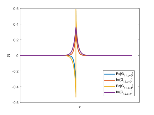
(b)

Figure 1: (a) Un-deformed $b=0$ and deformed $b=4$ Green function in Hermitian case $\alpha=0$ with fixed $J=1,\mu=0.3,T=0.01,\kappa=0$. (b) Un-deformed $b=0$ and deformed $b=4$ Green function in Hermitian case $\alpha=0.3$ with fixed $J=1,\mu=0.3,T=0.01,\kappa=0$.

As shown in Fig.1, the $T\bar{T}$ deformation will affect the Green function a shifting on correlation decay rates.

Substituting the saddle point solutions into the action, we obtain the free energy

$$\frac{F}{N}= -T\frac{\log Z}{N}=T\frac{S_{eff}}{N}$$

$$= -T\bigg{[}2\log 2+\sum_{\omega_{n}}\log\frac{D(i\omega_{n},\alpha)}{(i\omega_{n})^{2}}+\sum_{\omega_{n}}\bigg{(}\frac{3}{4}\Sigma_{LL}(i\omega_{n},\alpha)$$

$$G_{LL}(i\omega_{n},\alpha)+\frac{3}{4}\Sigma_{RR}(i\omega_{n},\alpha)G_{RR}(i\omega_{n},\alpha)+\frac{3}{4}\Sigma_{LR}(i\omega_{n},\alpha)$$

$$G_{RL}(i\omega_{n},\alpha)+\frac{3}{4}\Sigma_{RL}(i\omega_{n},\alpha)G_{LR}(i\omega_{n},\alpha)\bigg{)}\bigg{]}\,.$$ (87)

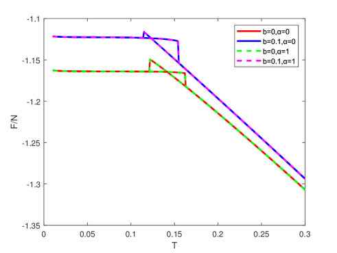
(a)

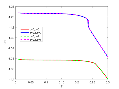
(b)

Figure 2: (a) Un-deformed $b=0$ and $T\bar{T}$ deformation $b=0.1$ on the free energy as a function of T with $J=1,\mu=0.3,\kappa=0$ in Hermitian case $\alpha=0$ and non-Hermitian case $\alpha=1$. (b) Un-deformed $b=0$ and $T\bar{T}$ deformation $b=0.1$ on the free energy as a function of T with $J=1,\mu=0.7,\kappa=0$ in Hermitian case $\alpha=0$ and non-Hermitian case $\alpha=1$.

In order to plot the free energy in Fig.2, we decrease the temperature first, and then increase the temperature back to the high temperature. After $T\bar{T}$ deformation, the free energy in wormhole phase will increase, and the black hole entropy also increase due to the larger slope. And this is exactly correlate to Nambu-Goto form of the Hamiltonian and the irrelevant property of $T\bar{T}$ deformation. The transition critical point, the non-Hermitian parameter take the phase structure closer to the second-order critical point, and the $T\bar{T}$ deformation make the phase transition more distinguishable as shown in Fig.2(b). And the deformed theory also moves over the second-order critical point as parameter $\mu$ increasing.

Note that the $T\bar{T}$ deformation also change the thermal phase structure, we have also plotted the phase diagram in detail with free energy.

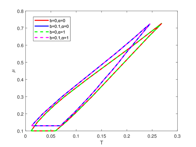
(a)

Figure 3: (a) Un-deform $b=0$ and $T\bar{T}$ deformation $b=0.1$ on phase diagram with $J=1,\kappa=0$.

The phase diagram with dependence on $\mu$ and T is numerically plotted in Fig.3, At small T and large $\mu$, the coupled system holographically dual to an eternal traversable wormhole. At large T and small $\mu$, the system reduces to two gapless black hole phase. Our results show that $T\bar{T}$ deformation decreases the range of coexistence region between wormhole phase and black hole phase as reparameterization $J$ .And it shifts the transition critical points in both Hermitian and non-Hermitian case. As deformation parameter $\lambda>0$, interaction $\mu$ also shifts to a small one in [7]. And non-Hermitian parameter does not change the effects of $T\bar{T}$ deformation. We have proved that the wormhole-black hole thermodynamic structure is robust not only in a Hermitian two coupled SYK model, but also in a non-Hermitian two coupled SYK model under the $T\bar{T}$ deformation.

VI.Revival dynamic

In this section, we investigate the dynamical property. Revival dynamic could be obtained from Lorentzian-time Green function in a Euclidean Keldysh time contour [42]. It is also convenient to introduce a Lorentz Wightman correlation function

$$G_{AB}^{>}\left(t_{1},t_{2}\right)=-iG_{AB}\left(it_{1}^{-},it_{2}^{+}\right)=-i\underset{\epsilon\rightarrow+0}{\lim}\left<\psi_{A}\left(\epsilon+it_{1}\right)\psi_{B}\left(-\epsilon+it_{2}\right)\right>,$$

$$G_{AB}^{<}\left(t_{1},t_{2}\right)=-G_{BA}^{>}\left(t_{2},t_{1}\right),$$ (88)

Retarded and Advanced Green function are also important in real time calculation

$$G_{AB}^{R}\left(t_{1},t_{2}\right)=\theta\left(t_{1}-t_{2}\right)\left(G_{AB}^{>}\left(t_{1},t_{2}\right)-G_{AB}^{<}\left(t_{1},t_{2}\right)\right),$$

$$G_{AB}^{A}\left(t_{1},t_{2}\right)=\theta\left(t_{2}-t_{1}\right)\left(G_{AB}^{<}\left(t_{1},t_{2}\right)-G_{AB}^{>}\left(t_{1},t_{2}\right)\right).$$ (89)

The Schwinger-Dyson equation in Lorentzian time version are constructed by real time correlation function and its retarded or advanced components

$$i\partial_{t_{1}}G_{AB}^{>}\left(t_{1},t_{2}\right)=\mu_{AC}G_{CB}^{>}\left(t_{1},t_{2}\right)+\int{dt\left(\varSigma_{AC}^{R}\left(t_{1},t\right)G_{CB}^{>}\left(t,t_{2}\right)+\varSigma_{AC}^{>}\left(t_{1},t\right)G_{CB}^{A}\left(t,t_{2}\right)\right)},$$

$$i\partial_{t_{1}}G_{AB}^{R}\left(t_{1},t_{2}\right)-\mu_{AC}G_{CB}^{R}\left(t_{1},t_{2}\right)-\int{dt\left(\varSigma_{AC}^{R}\left(t_{1},t\right)G_{CB}^{R}\left(t,t_{2}\right)+\varSigma_{AC}^{A}\left(t_{1},t\right)G_{CB}^{A}\left(t,t_{2}\right)\right)}=\delta_{AB}\delta\left(t_{1}-t_{2}\right),$$ (90)

with self energy term

$$\varSigma_{AB}^{>}\left(t_{1},t_{2}\right)=36J^{2}G_{AB}^{>}\left(t_{1},t_{2}\right)G_{AB}^{>}\left(t_{1},t_{2}\right)G_{BA}^{>}\left(t_{2},t_{1}\right),$$

$$\varSigma_{AB}^{R}\left(t_{1},t_{2}\right)=\theta\left(t_{1}-t_{2}\right)\left(\varSigma_{AB}^{>}\left(t_{1},t_{2}\right)+\varSigma_{BA}^{>}\left(t_{2},t_{1}\right)\right).$$ (91)

The Fourier transformation equation reduce to

$$G_{AB}^{R}\left(\omega\right)=\frac{\left(\omega-\kappa\right)\delta_{AB}-\varSigma_{BA}^{R}\left(\omega\right)-i\mu e^{-2\alpha}\delta_{aL}\delta_{bR}+i\mu e^{2\alpha}\delta_{aR}\delta_{bL}}{\left(\omega-\kappa-\varSigma_{LL}\right)\left(\omega-\kappa-\varSigma_{RR}\right)-\left(i\mu e^{-2\alpha}-\varSigma_{LR}\right)\left(-i\mu e^{2\alpha}-\varSigma_{RL}\right)}.$$ (92)

In Lorentz time form, an additional exponential divergence could be generated from Fourier transformation with real hyperbolic terms. We should introduce the thermal decay rate and its time strip by frequency partition function with statistical temperature T

$$G_{AB}^{>}\left(\omega\right)=\frac{G_{AB}^{R}\left(\omega\right)-\left(G_{BA}^{R}\left(\omega\right)\right)^{*}}{1+\exp\left(-\beta\omega\right)}.$$ (93)

In Hermitian system, Lorentz-time Green function could be reduced to pure real or pure imagine,

$$G_{LL}^{>}\left(\omega\right)=\frac{2i\mathrm{Im}\left(G_{LL}^{R}\left(\omega\right)\right)}{1+\exp\left(-\beta\omega\right)},$$

$$G_{LR}^{>}\left(\omega\right)=\frac{2\mathrm{Re}\left(G_{LR}^{R}\left(\omega\right)\right)}{1+\exp\left(-\beta\omega\right)}.$$ (94)

$T\bar{T}$ deformation in Lorentz time could be performed exactly the same way in Euclidean situation, except switching original Euclidean representation to the Lorentzian one. From the $T\bar{T}$ flow in Lorentz-time action with corresponding Schwinger-Dyson(SD) equations and correlation function, the auxiliary field we have introduced before in Euclidean space time turns out to be

$$\begin{split}i\frac{S_{total}}{N}&=i\frac{S_{L}+S_{R}+S_{int}}{N}=\log\det\left(\omega\delta_{AB}-\varSigma_{AB}\left(\omega\right)\right)\\ &-\frac{1}{2}\int{d\tau d\tau^{\prime}}\sum_{AB}{\left[\varSigma_{AB}\left(\tau,\tau\prime\right)G_{BA}\left(\tau\prime,\tau\right)-\frac{2^{2q-2}J_{AB}^{2}}{q^{2}}G_{AB}^{q}\left(\tau,\tau\prime\right)G_{BA}^{q}\left(\tau\prime,\tau\right)\right]}\\ &+\frac{i\mu}{2}\int{d\tau d\tau^{\prime}}\left[G_{LR}\left(\tau,\tau^{\prime}\right)\delta\left(\tau-\tau^{\prime}\right)-G_{RL}\left(\tau^{\prime},\tau\right)\delta\left(\tau^{\prime}-\tau\right)\right]\\ &-\frac{\kappa}{2}\int{d\tau d\tau^{\prime}}\left[G_{LL}\left(\tau,\tau^{\prime}\right)\delta\left(\tau-\tau^{\prime}\right)+G_{RR}\left(\tau^{\prime},\tau\right)\delta\left(\tau^{\prime}-\tau\right)\right].\end{split}$$ (95)

In order to reduce additional elements with Euclidean symbol, it is nature to transform the function along another Keldysh contour into Lorentzian

$$\varSigma=\varSigma^{>}-\varSigma^{R},$$

$$G=G^{A}+G^{>},$$ (96)

with a simple reparameterization J$\zeta$ could be represented by Lorentz coordinate

$$\begin{split}\zeta^{-2}&=1+b\int{d\tau}\left(\sum_{AB}{G_{AB}^{q}\left(\tau\right)G_{BA}^{q}\left(-\tau\right)}+i\mu^{\prime}\left(-e^{2\alpha}G_{LR}\left(\tau\right)\delta\left(-\tau\right)+e^{-2\alpha}G_{RL}\left(\tau\right)\delta\left(-\tau\right)\right)\right.\\ &\left.-\kappa^{\prime}\left(G_{LL}\left(\tau\right)\delta\left(-\tau\right)+G_{RR}\left(\tau\right)\delta\left(-\tau\right)\right)\right).\end{split}$$ (97)

Auxiliary parameter $\zeta$ should be switched to real time patch with real time SD equation

$$\begin{split}\zeta^{-2}&=1+b\int{dt}\left(\sum_{AB}{G_{AB}^{q}\left(t\right)G_{BA}^{q}\left(-t\right)}+\mu^{\prime}\left(-e^{2\alpha}G_{LR}\left(t\right)\delta\left(-t\right)+e^{-2\alpha}G_{RL}\left(t\right)\delta\left(-t\right)\right)\right)\\ &\left.+i\kappa^{\prime}\left(G_{LL}\left(t\right)\delta\left(-t\right)+G_{RR}\left(t\right)\delta\left(-t\right)\right)\right).\end{split}$$ (98)

After involving the contoured function, $\zeta$ are now written in the real time correlation and its advanced component

$$\begin{split}\zeta^{-2}&=1+b\int{dt}\left(\sum_{AB}{\left(G_{AB}^{A}\left(t\right)+G_{AB}^{>}\left(t\right)\right)^{q}\left(G_{BA}^{A}\left(-t\right)+G_{BA}^{>}\left(-t\right)\right)^{q}}\right.\\ &+\mu^{\prime}\left(-e^{2\alpha}\left(G_{LR}^{A}\left(t\right)+G_{LR}^{>}\left(t\right)\right)\delta\left(-t\right)+e^{-2\alpha}\left(G_{RL}^{A}\left(t\right)+G_{RL}^{>}\left(t\right)\right)\delta\left(-t\right)\right)\\ &\left.-i\kappa^{\prime}\left(\left(G_{LL}^{A}\left(t\right)+G_{LL}^{>}\left(t\right)\right)\delta\left(-t\right)+\left(G_{RR}^{A}\left(t\right)+G_{RR}^{>}\left(t\right)\right)\delta\left(-t\right)\right)\right).\end{split}$$ (99)

According to transmission symmetry between retarded and advanced correlation, we simply shift the expression into retarded form

$$\begin{split}\zeta^{-2}&=1+b\int{dt}\left(\sum_{AB}{\left(-G_{AB}^{R}\left(-t\right)+G_{AB}^{>}\left(t\right)\right)^{q}\left(-G_{BA}^{R}\left(t\right)+G_{BA}^{>}\left(-t\right)\right)^{q}}\right.\\ &+\mu^{\prime}\left(-e^{2\alpha}\left(-G_{LR}^{R}\left(-t\right)+G_{LR}^{>}\left(t\right)\right)\delta\left(-t\right)+e^{-2\alpha}\left(-G_{RL}^{R}\left(-t\right)+G_{RL}^{>}\left(t\right)\right)\delta\left(-t\right)\right)\\ &\left.-i\kappa^{\prime}\left(\left(-G_{LL}^{R}\left(-t\right)+G_{LL}^{>}\left(t\right)\right)\delta\left(-t\right)+\left(-G_{RR}^{R}\left(-t\right)+G_{RR}^{>}\left(t\right)\right)\delta\left(-t\right)\right)\right).\end{split}$$ (100)

We used to utilize Fourier transformation to detour infinite proper time integral. However, Matsubara Fermion frequencies in usual many-body quantum system recover a divergent result in Lorentz-time equations. Numerically, a real-time cut off could be preformed without violating the limited causality in both frequency space and Lorentz time space. Preforming a long-time cut off would be a good attempt for numerical approximation method[38]. The discrete numerical time scales are now given by

$$t_{m}=mt_{\max},$$

$$m=\left(-\varLambda,-\varLambda+1,\cdots,\varLambda-1\right)/\varLambda.$$ (101)

conjugated discrete frequency is

$$\omega_{n}=\pi n/t_{\max},$$

$$n=\left(-\varLambda,-\varLambda+1,\cdots,\varLambda-1\right).$$ (102)

After discrete Fourier transformation, we obtain a frequency represented $\zeta$

$$\begin{split}\zeta^{-2}&=1+b/\left(2t_{\max}\right)\sum_{\omega_{n}}{\left(\sum_{AB}{\left(-G_{AB}^{R}\left(-\omega_{n}\right)+G_{AB}^{>}\left(\omega_{n}\right)\right)^{q}\left(-G_{BA}^{R}\left(-\omega_{n}\right)+G_{BA}^{>}\left(\omega_{n}\right)\right)^{q}}\right.}\\ &+\mu^{\prime}\left(-e^{2\alpha}\left(-G_{LR}^{R}\left(\omega_{n}\right)+G_{LR}^{>}\left(\omega_{n}\right)\right)+e^{-2\alpha}\left(-G_{RL}^{R}\left(\omega_{n}\right)+G_{RL}^{>}\left(\omega_{n}\right)\right)\right)\\ &\left.-i\kappa^{\prime}\left(\left(-G_{LL}^{R}\left(\omega_{n}\right)+G_{LL}^{>}\left(\omega_{n}\right)\right)+\left(-G_{RR}^{R}\left(\omega_{n}\right)+G_{RR}^{>}\left(\omega_{n}\right)\right)\right)\right).\end{split}$$ (103)

Notice that the temperature T dependent in Euclidean time zeta is somehow replaced by inverse maximal Lorentz time cut off $1/2t_{\max}$. The temperature now appears in statistical real time decay spectral. However, this numerical relation $1/2t_{\max}$ is not arbitrary, since the time cut off $1/2t_{\max}$ and inverse temperature $\beta$ should match with each other. We numerically calculate the real time propagator in Fig.4. And it is significant to choose the critical transition point between wormhole phase and two-black hole phase. More explicitly, we have choose the maximal transmission amplitude $Trans=\left|2G_{LR}\right|$ is close to 1. The $T\bar{T}$ deformation shifts the thermal phase structure as we calculate in previous section. The result of wormhole-like solution at transition point make the oscillation vanish and gradually transforms into black hole after utilizing the $T\bar{T}$ deformation. Notice that the wormhole revival function with $\mu=0.3$ greatly enhance the $G_{LR}$ component and replace the role of $G_{LL}$ does with $\mu=0.1$ or smaller. We shall focus on the dynamical decays for interaction parts. In fig.4 (b) and (d), the deformation will shift the phase diagram from original position, and the temperature here is no longer on transition point and the density is not convergent. In non-Hermitian case, the symmetry between the propagator of L-R and R-L is broken. In fig.4 (c) and (d), the $T\bar{T}$ deformation b=0.001 will slightly decrease the oscillation. And this result agrees with phase structure in last section.

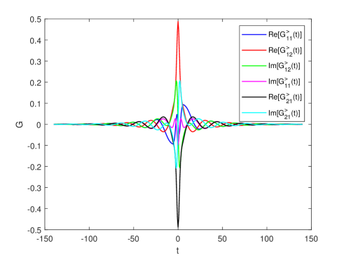
(a)

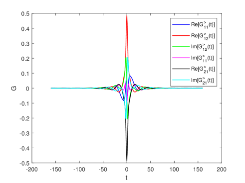
(b)

(c)

(d)

Figure 4: Revival dynamic in wormhole-like critical point with $J=1/3,\mu=0.3,T=0.131,\lambda=200000$ (a) Real time propagator with Hermitian $\alpha=0,t_{max}=140000,b=0$. (b) Real time propagator with Hermitian $\alpha=0,t_{max}=160000,b=0.001$.(c) Real time propagator with non-Hermitian $\alpha=0.3,t_{max}=140000,b=0$. (d) Real time propagator with non-Hermitian $\alpha=0.3,t_{max}=160000,b=0.001$.

VII.Conclusion

We have investigated a $T\bar{T}$ deformation on two coupled SYK model, and its non-Hermitian prolongation. By analysing the energy excitation on ground state, we have actually proved that the $T\bar{T}$ deformation has no influence on ground state, since there is no excitation in original energy-momentum tensor flow. $T\bar{T}$ deformation on overlap could be transform into a shifting of interaction $\mu$ without changing the overlap numerical results. The phase transition from the wormhole phase to the two black hole phase still exists in a non-Hermitian two coupled SYK model under $T\bar{T}$ deformation.

$T\bar{T}$ deformation in AdS spacetime has been proved to be a radial cut off. However, this physical explain does not coexist with any additional matter field, because the cut-off metric does not contain a $T\bar{T}$ flow equation on sphere. When we focus on the cut off space, additional parts outside the cut off sphere would be indistinguishable from NAdS boundary term. Energy-momentum flow and its trigger $T\bar{T}$ operator on cut off radial sphere should be exactly the same form as $T\bar{T}$ deformation. We also obtain the same result in coupled SYK model with similar mathematical expression. And non-Hermitian effects break the symmetry of entangle wormhole between left and right copies.

In low energy limit, the effective action emerges a conformal symmetry and reduces to Schwarzian form, which leads to an analytical holography property. We directly introduce the $T\bar{T}$ deformation on its mathematical flow equation formally with a Schwarzian time reparameterization coordinate dependence. And we obtain the deformed Schwarzian form for both dilaton geometry in gravity side and correlation function in quantum model. We found that the deformation of large $N$ theory could be reparametrized and shows the same result as a shifting the model coupling constant $J$,$\mu$ and $\kappa$. It also leads to a increasing effect of free energy in wormhole phase. The free energy under deformation also preform a shift in black hole phase and change the phase structure. In Lorentz time, we have investigated the Green function in black hole and wormhole phase. Since the correlation function of wormhole should be oscillating, and saddle point equation would be an approximate method for wormhole solution. In black hole phase, the numerical limit $t_{max}$ increases and it is numerically equal to decrease the temperature to approach a wormhole oscillation solution. The phase structure represented by real time green function also preform a shifting after utilizing the $T\bar{T}$ deformation. In our result, wormhole solution gradually turns to be black hole as deformation parameter increase.

References

[1]
Juan, Maldacena, and Douglas Stanford. ”Remarks on the sachdev-ye-kitaev model.” Physical Review D 94.10 (2016): 106002.
[2]
Subir Sachdev and Jinwu Ye, “Gapless spin-fluid ground
state in a random quantum Heisenberg magnet,” Phys.
Rev. Lett. 70, 3339–3342 (1993).
[3]
Subir Sachdev, “Bekenstein-hawking entropy and strange
metals,” Phys. Rev. X 5, 041025 (2015).
[4]
Alexei Kitaev, “A simple model of quantum holography,”
(2015), KITP Strings Seminar and Entanglement Program.
[5]
Juan, Maldacena, Douglas Stanford, and Zhenbin Yang. ”Conformal symmetry and its breaking in two-dimensional nearly anti-de Sitter space.” Progress of Theoretical and Experimental Physics 2016.12 (2016): 12C104.
[7]
Wenhe, Cai, Sizheng Cao, Xian-Hui Ge, Masataka Matsumoto and Sang-Jin Sin. ”Non-Hermitian quantum system generated from two coupled Sachdev-Ye-Kitaev models.” Physical Review D 106.10 (2022): 106010.
[8]
Song, He, and Zhuo-Yu Xian. ” deformation on multiquantum mechanics and regenesis.” Physical Review D 106.4 (2022): 046002.
[9]
Song He, Pak Hang Chris Lau, Zhuo-Yu Xian, Long Zhao. ”Quantum chaos, scrambling and operator growth in deformed SYK models.” Journal of High Energy Physics 2022.12 (2022): 1-32.
[10]
F. A. Smirnov and A. B. Zamolodchikov, On space of integrable quantum field theories,
Nucl. Phys. B915 (2017) 363–383 [1608.05499]
[11]
Zamolodchikov, Alexander B. ”Expectation value of composite field in two-dimensional quantum field theory.” arXiv preprint hep-th/0401146 (2004).
[12]
Cavaglià, Andrea, et al. ”-deformed 2D quantum field theories.” Journal of High Energy Physics 2016.10 (2016): 1-28.
[13]
Gross, David J., et al. ” in and quantum mechanics.” Physical Review D 101.2 (2020): 026011.
[14]
Gross, David J., et al. ”Hamiltonian deformations in quantum mechanics, and SYK.” arXiv preprint arXiv:1912.06132 (2019).
[15]
L. Castillejo, R. H. Dalitz and F. J. Dyson, Low’s scattering equation for the charged and neutral scalar theories,
Phys. Rev. 101 (1956) 453–458.
[16]
S. Dubovsky, R. Flauger and V. Gorbenko, Solving the Simplest Theory of Quantum Gravity,
JHEP 09 (2012) 133 [1205.6805]
[17]
R. Conti, L. Iannella, S. Negro and R. Tateo, Generalised Born-Infeld models, Lax operators and the perturbation,
JHEP 11 (2018) 007 [1806.11515].
[18]
R. Conti, S. Negro and R. Tateo, The perturbation and its geometric interpretation,
JHEP 02 (2019) 085 [1809.09593].
[19]
G. Hern´andez-Chifflet, S. Negro and A. Sfondrini, Flow Equations for Generalized Deformations, Phys. Rev. Lett. 124 (2020), no. 20 200601 [1911.12233].
[20]
O. Aharony, S. Datta, A. Giveon, Y. Jiang and D. Kutasov, Modular invariance and uniqueness of deformed CFT,
JHEP 01 (2019) 086 [1808.02492].
[21]
Bonelli, Giulio, Nima Doroud, and Mengqi Zhu. ”TT¯ -deformations in closed form.” Journal of High Energy Physics 2018.6 (2018): 1-17.
[22]
Aharony, Ofer, and Zohar Komargodski. ”The effective theory of long strings.” Journal of High Energy Physics 2013.5 (2013): 1-26.
[23]
Gendenshteĭn, L. É., and Il’ya Valentinovich Krive. ”Supersymmetry in quantum mechanics.” Soviet Physics Uspekhi 28.8 (1985): 645.
[24]
Taylor, Marika. ”TT deformations in general dimensions.” arXiv preprint arXiv:1805.10287 (2018).
[25]
R. Conti, S. Negro and R. Tateo, Conserved currents and s irrelevant deformations of 2D integrable field theories,
JHEP 11 (2019) 120 [1904.09141].
[26]
A. B. Zamolodchikov, Expectation value of composite field T anti-T in two-dimensional quantum field theory,
hep-th/0401146.
[27]
L. McGough, M. Mezei and H. Verlinde, Moving the CFT into the bulk with ,
JHEP 04 (2018) 010 [1611.03470].
[28]
T. Hartman, J. Kruthoff, E. Shaghoulian and A. Tajdini, Holography at finite cutoff with a T 2 deformation,
JHEP 03 (2019) 004 [1807.11401].
[29]
P. Caputa, S. Datta and V. Shyam, Sphere partition functions & cut-off AdS,
JHEP 05 (2019) 112 [1902.10893].
[30]
V. Shyam, Background independent holographic dual to deformed CFT with large central charge in 2 dimensions,
JHEP 10 (2017) 108 [1707.08118].
[31]
S. Dubovsky, V. Gorbenko and G. Hernandez-Chifflet, partition function from topo logical gravity,
JHEP 09 (2018) 158 [1805.07386].
[33]
C. Teitelboim, “Gravitation and Hamiltonian Structure in Two Space-Time
Dimensions,” Phys. Lett. B126 (1983) 41–45.
[34]
Juan, Maldacena, and Douglas Stanford. and Z. Yang, “Conformal symmetry and its breaking in
two dimensional Nearly Anti-de-Sitter space,” PTEP 2016 no. 12, (2016) 12C104.
[35]
A. Almheiri and J. Polchinski, “Models of AdS2 backreaction and holography,”
JHEP 11 (2015) 014.
[36]
Hartman, Thomas, et al. ”Holography at finite cutoff with a T2 deformation.” Journal of High Energy Physics 2019.3 (2019): 1-29.
[37]
De Rham, Claudia, and Andrew Matas. ”Ostrogradsky in theories with multiple fields.” Journal of Cosmology and Astroparticle Physics 2016.06 (2016): 041.
[38]
Nosaka, Tomoki, and Tokiro Numasawa. ”Chaos exponents of SYK traversable wormholes.” Journal of High Energy Physics 2021.2 (2021): 1-44
[39]
Sahoo, Sharmistha, et al. ”Traversable wormhole and Hawking-Page transition in coupled complex SYK models.” Physical Review Research 2.4 (2020): 043049.
[40]
Wenhe, Cai, Xian-Hui Ge, and Guo-Hong Yang. ”Diffusion in higher dimensional SYK model with complex fermions.” Journal of High Energy Physics 2018.1 (2018).
[41]
Davison, Richard A., et al. ”Thermoelectric transport in disordered metals without quasiparticles: The Sachdev-Ye-Kitaev models and holography.” Physical Review B 95.15 (2017): 155131.
[42]
Plugge, Stephan, Étienne Lantagne-Hurtubise, and Marcel Franz. ”Revival dynamics in a traversable wormhole.” Physical review letters 124.22 (2020): 221601.
[43]
Sizheng, Cao, Yi-Cheng Rui, and Xian-Hui Ge. ”Thermodynamic phase structure of complex Sachdev-Ye-Kitaev model and charged black hole in deformed JT gravity.” arXiv preprint arXiv:2103.16270 (2021).