Markov Chain Monte Carlo Data Association
for Sets of Trajectories

Abstract

This paper considers a batch solution to the multi-object tracking problem based on sets of trajectories. Specifically, we present two offline implementations of the trajectory Poisson multi-Bernoulli mixture (TPMBM) filter for batch data based on Markov chain Monte Carlo (MCMC) sampling of the data association hypotheses. In contrast to online TPMBM implementations, the proposed offline implementations solve a large-scale, multi-scan data association problem across the entire time interval of interest, and therefore they can fully exploit all the measurement information available. Furthermore, by leveraging the efficient hypothesis structure of TPMBM filters, the proposed implementations compare favorably with other MCMC-based multi-object tracking algorithms. Simulation results show that the TPMBM implementation using the Metropolis-Hastings algorithm presents state-of-the-art multiple trajectory estimation performance.

I Introduction

Multi-object tracking (MOT) refers to the joint estimation of the number of objects and the object trajectories from noisy sensor measurements [1, 2, 3]. Previous works on MOT with trajectory estimation include vector-type methods and set-type methods using labels. The former describes the multi-object states by vectors and constructs trajectories by linking a state estimate with a previous one, while the latter forms trajectories by linking state estimates with the same label. Most of these works focus on the task of estimating the current object states based on all previous measurements, and the main challenge is to handle the data association problem, i.e. to determine the associations between measurements and objects.

In this paper, our focus is on a batch formulation of MOT by exploiting all the measurement information in the time interval of interest. The fact that offline algorithms generally do not have to be as computationally efficient as online algorithms enables us to revisit and update data associations at previous time steps in light of new observations and thereby improve the estimation of past object states. These offline algorithms are important for trajectory analytics, with various applications in, e.g. cell tracking, sports athletes tracking, and training data collection for learning-based MOT algorithms.

The main challenge in batch MOT implementations is to handle the data associations across the entire time interval of interest, where each such global data association can be interpreted as a parition of the sequence of sets of measurements into false alarms and clusters of measurements from different time steps originating from the same object. Finding the most likely global data association is a large-scale multidimensional assignment problem. Conventional solutions to this multi-scan data association problem mainly reply on binary programming solvers based on Lagrangian relaxation [4, 5]. However, these methods can generally only handle data associations up to a few time steps, and thus they typically consider sliding window implementations.

I-A Batch MOT with MCMC Sampling

In this paper, we address this large scale multi-scan data association problem using Markov chain Monte Carlo (MCMC) sampling. Several MCMC methods have been developed for MOT with image sequences where the proposal distributions for drawing samples of data associations are tailored to image detections [6, 7, 8, 9]. Different from these works, we focus on MOT with the standard multi-object models for point objects [10]. This means that each global data association represents a measurement partition where each cluster of measurements originating from the same object is a collection of at most one measurement at different time steps.

An early work using MCMC sampling to solve the multi-scan data association problem for point objects is [11], where the Metropolis-Hastings (MH) algorithm is used to iteratively sample data associations from well-designed proposal distributions, incorporated with certain domain-specific knowledge. The MCMC sampling method in [11] has later been combined with a particle Gibbs algorithm in [12] for model parameter estimation. The problem of MOT with modelling uncertainties was also addressed in [13] using MH sampling and the possibility theory [14]. The MCMC sampling method in [11] has also been extended in [15] to consider a particle filter-based implementation with more sophisticated proposal distributions. Recently, another MOT batch solution has been presented in [16], where the multi-scan data association problem is solved using Gibbs sampling [16].

In the above works, conditioned on a global data association hypothesis, objects have deterministic existences in the multi-object density representation. Therefore, object birth and death events need to be sampled to determine trajectory start and end times, resulting in a significantly increased sampling space. In principle, in batch MOT the objective is to compute the posterior density distribution of the set of trajectories, which captures all the information about the trajectories. Conditioned on a specific global data association, we would like to reason about the existence probability of each detected trajectory and the probabilities that the trajectory starts and ends at certain time steps. This can be achieved by considering MOT based on sets of trajectories [17].

I-B Trajectory Poisson multi-Bernoulli Mixtures for MOT

A variety of multi-object trackers based on sets of trajectories has been developed [18, 19, 20, 21, 17, 22, 23, 24, 25, 26, 27, 28, 29], showing promising performance on various tasks. For standard multi-object models with Poisson point process (PPP) birth [10], the analytic solution to MOT based on sets of trajectories is given by the trajectory Poisson multi-Bernoulli mixture (PMBM) filter [19], which is an extension of the PMBM filter [30, 31] for sets of objects to sets of trajectories. The trajectory PMBM (TPMBM) filter has achieved state-of-the-art trajectory estimation performance for both point [19, 20] and extended objects [23, 25].

The trajectory PMBM (TPMBM) filter enjoys an efficient multi-object density representation via the probabilistic existence of each detected trajectory and its start/end times. Importantly, in the TPMBM posterior we have exactly one global hypothesis for every possible partition of the measurements. As a comparison, for multi-object density representations that use deterministic object existences, the number of global hypotheses exponentially increases with the number of potential objects, resulting in a less efficient hypothesis structure [31].

Furthermore, by modelling the set of undetected trajectories, which are hypothesized to exist but have not been detected, using a PPP in TPMBM, one is able to reason about the start time and states of a trajectory before it was detected for the first time. The TPMBM strategy to model undetected objects follows naturally from the MOT model assumptions and the PPP birth, but undetected objects are still often ignored by other algorithms that use a PPP birth, e.g. [11, 15]. Another popular MOT birth model is the multi-Bernoulli (MB) process, which is used in [16] to implicitly model undetected objects. However, the MB birth model sets a maximum number of newborn objects at each time step, which may not be suitable for many scenarios. The TPMBM filtering recursions can also be easily adapted to the MB birth model by setting the Poisson intensity to zero and adding Bernoulli components of the MB birth in the prediction step [22].

In TPMBM filtering, we can improve past state estimates in the trajectories via smoothing-while-filtering [19, 20]. In principle, the TPMBM filters can produce optimal trajectory estimates if they are implemented without approximations (and an optimal trajectory estimator is used). However, in practice, we have to resort to some approximation methods, such as pruning, to keep the computational complexity of the filter at a tractable level. This means that the performance of an online TPMBM filter implementation may decrease when there are too many feasible global data association hypotheses that cannot be effectively enumerated. This motivates us to consider batch TPMBM implementations, where the multi-scan data association problem is solved using MCMC sampling.

I-C Contributions

None of the above MOT algorithms that use MCMC sampling for data association [11, 15, 16] have a hypothesis structure that is as efficient as PMBM, nor do they consider the posterior densities on sets of trajectories. Moreover, these existing methods are unsuitable for the TPMBM density representation in their current form. This paper aims at bridging this gap in the literature, and its specific contributions include:

1. We present two batch TPMBM implementations based on MCMC sampling of data association hypotheses for point object tracking: one using the Gibbs sampling, and the other using the Metropolis-Hastings (MH) algorithm. The proposed implementations are able to leverage the efficient hypothesis structure of PMBM and the compact trajectory density representation.

2. In the TPMBM implementation using Gibbs sampling, we adopt a blocked Gibbs sampling strategy to jointly sample a group of data association variables at each time step, making it suitable for Poisson birth. We also show that the conditional distribution in Gibbs sampling can be evaluated in a computationally efficient manner.

3. In the TPMBM implementation using MH sampling, we show that simple yet flexible proposal distributions are sufficient for sampling the data association variables as compared to the complex designs in [11, 15]. This is possible since uncertainties on trajectory existence and start/end times are captured in the trajectory Bernoulli densities. In addition, we leverage Gibbs sampling when designing the track update move.

4. The proposed batch TPMBM implementations are compared to several state-of-the-art multi-object smoothing methods. This comparative analysis is conducted in a challenging scenario where objects move in proximity, and it includes an extensive ablation study. The results show that TPMBM implementation using MH sampling has the best trajectory estimation performance.

The rest of the paper is organized as follows. Models and concepts on sets of trajectories are introduced in Section II. We present the TPMBM filtering recursions in Section III and formulate the batch MOT problem using TPMBM in Section IV. Section V presents the two batch TPMBM implementations using MCMC sampling. Simulations and results are shown in Section VI, and conclusions are drawn in Section VII.

II Background

Let $x_{k}\in\mathbb{R}^{n_{x}}$ denote a single object state with dimension $n_{x}$ at time step $k$, and the multi-object state at time step $k$ is a set of single object states $\mathbf{x}_{k}\in\mathcal{F}(\mathbb{R}^{n_{x}})$, where $\mathcal{F}(D)$ denotes the set of finite subsets of space $D$. Let $z_{k}\in\mathbb{R}^{n_{z}}$ denote a single measurement with dimension $n_{z}$ at time step $k$. The set of $m_{k}$ measurements at time step $k$ is $\mathbf{z}_{k}=\{z_{k}^{1},\dots,z_{k}^{m_{k}}\}\in\mathcal{F}(\mathbb{R}^{n_{z}})$, and the sequence of measurement sets received up to and including time step $k$ is $\mathbf{z}_{1:k}=(\mathbf{z}_{1},\dots,\mathbf{z}_{k})$.

The Dirac and Kronecker delta functions centered at $x$ are respectively represented using $\delta_{x}(\cdot)$ and $\delta_{x}[\cdot]$. The indicator function for a given set $D$ is denoted by $1_{D}(\cdot)$, and the inner product $\int f(x)g(x)dx$ between two functions $f(x)$ and $g(x)$ is denoted by $\langle f,g\rangle$. The cardinality of set $\mathbf{x}$ is denoted $|\mathbf{x}|$.

II-A Trajectory Representation

A trajectory is a finite sequence of single object states at consecutive time steps. It can be denoted as $X=(\beta,\varepsilon,x_{\beta:\varepsilon})$, where $\beta$ is the time step trajectory $X$ starts, $\varepsilon$ is the time step trajectory $X$ ends, and $x_{\beta:\varepsilon}$ is the sequence of object states $(x_{\beta},x_{\beta+1},\dots,x_{\varepsilon-1},x_{\varepsilon})$ in trajectory $X$ with length $\varepsilon-\beta+1$ [19]. The trajectory space for trajectories up to time step $k$ is

$$\mathcal{T}_{k}=\uplus_{(\beta,\varepsilon)\in I_{k}}\{\beta\}\times\{\varepsilon\}\times\mathbb{R}^{n_{x}(\varepsilon-\beta+1)},$$

where $\uplus$ denotes union of disjoint sets and $I_{k}=\{(\beta,\varepsilon):1\leq\beta\leq\varepsilon\leq k\}$.

The single trajectory function factorizes as

$$p(X)=p(x_{\beta:\varepsilon}|\beta,\varepsilon)p(\beta,\varepsilon),$$

where $p(\beta,\varepsilon)$ is defined on $I_{k}$ for $X\in\mathcal{T}_{k}$. The integral of $p(X)$ is given by

$$\int_{\mathcal{T}_{k}}p(X)dX=\sum_{(\beta,\varepsilon)\in I_{k}}p(\beta,\varepsilon)\int p(x_{\beta:\varepsilon}|\beta,\varepsilon)dx_{\beta:\varepsilon}.$$

Given trajectories $X=(\beta,\varepsilon,x_{\beta:\varepsilon})$ and $X^{\prime}=(\beta^{\prime},\varepsilon^{\prime},x^{\prime}_{\beta^{\prime}:\varepsilon^{\prime}})$, the trajectory Dirac delta function is defined as

$$\delta_{X}\left[X^{\prime}\right]=\delta_{\beta}\left[\beta^{\prime}\right]\delta_{\varepsilon}\left[\varepsilon^{\prime}\right]\delta_{x_{\beta:\varepsilon}}\left(x^{\prime}_{\beta^{\prime}:\varepsilon^{\prime}}\right).$$

Trajectory functions are typically represented in a mixture form. Consider a trajectory function with $L$ components

$$p(X)=\sum_{l=1}^{L}\nu^{l}p^{l}\left(x_{\beta:\varepsilon}|\beta,\varepsilon\right)\delta_{b^{l}}\left[\beta\right]\delta_{e^{l}}\left[\varepsilon\right],$$ (1)

where the $l$-th component is characterized by a weight $\nu^{l}$ and state parameters $(b^{l},e^{l},p^{l}(\cdot))$ with $b^{l}\leq e^{l}$. If $\sum_{l=1}^{L}\nu^{l}=1$, then $p(X)$ is a trajectory density function. If $\sum_{l=1}^{L}\nu^{l}\geq 0$, then $p(X)$ is a trajectory intensity function. For a trajectory density function of the form (1), the probability mass function (pmf) of $(\beta,\varepsilon)$ is given by

$$p(\beta,\varepsilon)=\int p(X)dx_{\beta:\varepsilon}=\sum_{l=1}^{L}\nu^{l}\delta_{b^{l}}[\beta]\delta_{e^{l}}[\varepsilon].$$

The set of trajectories in the time interval $0:k$ is denoted as $\mathbf{X}_{k}\in\mathcal{F}(\mathcal{T}_{k})$. Integration over sets of trajectories and multi-trajectory densities are defined similarly as integration over sets of objects and multi-object densities, respectively, see [17] for their explicit expressions.

II-B Multi-Trajectory Models

We focus on the estimation of the set $\mathbf{X}_{k}$ of trajectories of all objects that have passed through the surveillance area at some point between time step $0$ and the current time step $k$. These include both trajectories of objects that are still present in the area at time step $k$ and trajectories of objects that were previously in the area but have left it at time step $k$. We consider the standard multi-object models with Poisson birth [10, Sec. 9.2.1], which is general and can be used to model, e.g. detection-type measurements collected by surveillance and tracking radars. The corresponding multi-trajectory models [19] are given as follows.

Each single trajectory $X=(\beta,\varepsilon,x_{\beta:\varepsilon})\in\mathbf{X}_{k}$ is detected with probability $p^{D}_{k}(X)=p^{D}(x_{\varepsilon})\delta_{k}[\varepsilon]$ and generates a single measurement with density $\ell(z|X)=\ell(z|x_{\varepsilon})$, or misdetected with probability $1-p^{D}_{k}(X)$. Here, $p^{D}(x)$ is the state-dependent object detection probability. Clutter measurements are modelled using a PPP with intensity function $\lambda^{C}(\cdot)$, independent of any objects and object-generated measurements.

Given the set $\mathbf{X}_{k}$ of all trajectories, each trajectory $X=(\beta,\varepsilon,x_{\beta:\varepsilon})\in\mathbf{X}_{k}$ survives with probability $p^{S}(X)=1$, with a transition density [20]

$$g_{k+1}\left(\beta^{\prime},\varepsilon^{\prime},x^{\prime}_{\beta^{\prime}:\varepsilon^{\prime}}|X\right)=\delta_{\beta}\left[\beta^{\prime}\right]$$

$$\times\begin{cases}\delta_{\varepsilon}\left[\varepsilon^{\prime}\right]\delta_{x_{\beta:\varepsilon}}\left(x^{\prime}_{\beta^{\prime}:\varepsilon^{\prime}}\right)&\varepsilon^{\prime}<k\\ \delta_{\varepsilon}\left[\varepsilon^{\prime}\right]\delta_{x_{\beta:\varepsilon}}\left(x^{\prime}_{\beta^{\prime}:\varepsilon^{\prime}}\right)\left(1-p^{S}(x_{\varepsilon})\right)&\varepsilon^{\prime}=k\\ \delta_{\varepsilon+1}\left[\varepsilon^{\prime}\right]\delta_{x_{\beta:\varepsilon}}\left(x^{\prime}_{\beta^{\prime}:\varepsilon^{\prime}-1}\right)p^{S}(x_{\varepsilon})g(x_{\varepsilon^{\prime}}|x_{\varepsilon})&\varepsilon^{\prime}=k+1,\end{cases}$$ (2)

where $p^{S}(x)$ is the object survival probability and $g(\cdot|x)$ is the object state transition density. The interpretation of $p^{S}(X)=1$ is that regardless of whether the trajectory ends, it remains in the set of trajectories. Note that the pmf of trajectory end time is encapsulated in the single trajectory density via (2).

The set ${\bf X}_{k+1}$ of trajectories is the union of alive (present in the area), dead (not present in the area), and new trajectories, which are born independently following a PPP with intensity

$$\lambda_{k+1}^{B}(X)=\delta_{k+1}[\beta]\delta_{k+1}[\varepsilon]\lambda^{B}(x_{k+1}),$$ (3)

where $\lambda^{B}(x_{k+1})$ is the PPP intensity of newborn objects. Note that new trajectories at time step $k+1$ have deterministic start and end time $k+1$.

III Trajectory PMBM

In this section, we review TPMBM densities and filtering recursions for the multi-trajectory models described in Section II-B. We also present the batch MOT problem formulation based on TPMBM.

III-A Trajectory PMBM Density

Given the sequence of measurements $\mathbf{z}_{1:k}$ and the multi-trajectory measurement and dynamic models in Section II-B, the density $f_{k^{\prime}|k}(\cdot)$ of the set of trajectories up to time step $k^{\prime}$, where $k^{\prime}\in\{k,k+1\}$, is a PMBM [31, 19], with

$$f_{k^{\prime}|k}({\bf X}_{k^{\prime}}) =\sum_{\mathbf{X}_{k^{\prime}}^{u}\uplus\mathbf{X}_{k^{\prime}}^{d}=\mathbf{X}_{k^{\prime}}}f^{u}_{k^{\prime}|k}\left(\mathbf{X}_{k^{\prime}}^{u}\right)f_{k^{\prime}|k}^{d}\left(\mathbf{X}_{k^{\prime}}^{d}\right),$$ (4)

$$f^{u}_{k^{\prime}|k}\left(\mathbf{X}_{k^{\prime}}^{u}\right) =e^{-\int\lambda_{k^{\prime}|k}^{u}(X)dX}\prod_{X\in\mathbf{X}^{u}_{k^{\prime}}}\lambda_{k^{\prime}|k}^{u}(X),$$ (5)

$$f_{k^{\prime}|k}^{d}\left(\mathbf{X}_{k^{\prime}}^{d}\right) =\sum_{a\in\mathcal{A}_{k^{\prime}|k}}w^{a}_{k^{\prime}|k}\sum_{\uplus_{l=1}^{n_{k^{\prime}|k}}\mathbf{X}^{l}_{k^{\prime}}=\mathbf{X}_{k^{\prime}}^{d}}\prod_{i=1}^{n_{k^{\prime}|k}}f^{i,a^{i}}_{k^{\prime}|k}\left(\mathbf{X}_{k^{\prime}}^{i}\right),$$ (6)

$$f^{i,a^{i}}_{k^{\prime}|k}\left(\mathbf{X}_{k^{\prime}}^{i}\right) =\begin{cases}1-r_{k^{\prime}|k}^{i,a^{i}}&\mathbf{X}_{k^{\prime}}^{i}=\emptyset\\ r_{k^{\prime}|k}^{i,a^{i}}f^{i,a^{i}}_{k^{\prime}|k}(X)&\mathbf{X}_{k^{\prime}}^{i}=\{X\}\\ 0&\text{otherwise},\end{cases}$$ (7)

where $f_{k|k}({\bf X}_{k})$ (with $k^{\prime}=k$) represents the filtering density at time step $k$ and $f_{k+1|k}({\bf X}_{k+1})$ (with $k^{\prime}=k+1$) represents the predicted density at time step $k+1$. From (4), one can observe that the TPMBM is the union of two independent sets: a trajectory PPP (5) with Poisson intensity $\lambda^{u}_{k^{\prime}|k}(\cdot)$ that represents undetected trajectories, and a trajectory multi-Bernoulli mixture (MBM) (6) that represents trajectories that have been detected at some point up to and including time step $k$. In the PMBM filtering recursion, each received measurement creates a new Bernoulli component, and at time step $k^{\prime}$ the MBM (6) has $n_{k^{\prime}|k}$ Bernoulli components. Full details on the TPMBM filtering recursion are provided in [19].

A global (data association) hypothesis can be interpreted as a partition of the batch measurements $\mathbf{z}_{1:k}$ into at most $n_{k^{\prime}|k}$ non-empty, mutually disjoint subsets originated from the same potential object [30, Def. 2]. Here a global hypothesis is denoted as $a=(a^{1},\dots,a^{n_{k^{\prime}|k}})\in\mathcal{A}_{k^{\prime}|k}$, where for the $i$-th Bernoulli component, $a^{i}\in\{1,\dots,h^{i}_{k^{\prime}|k}\}$ indexes the local hypothesis and $h^{i}_{k^{\prime}|k}$ is the number of local hypotheses. The $i$-th Bernoulli component with local hypothesis $a^{i}$ has weight $w_{k^{\prime}|k}^{i,a^{i}}$ and density $f_{k^{\prime}|k}^{i,a^{i}}(\cdot)$, parameterized by probability of existence $r^{i,a^{i}}_{k^{\prime}|k}$ and single trajectory density $f_{k^{\prime}|k}^{i,a^{i}}(X)$. The weight of global hypothesis $a$ is $w^{a}_{k^{\prime}|k}\propto\prod_{i=1}^{n_{k^{\prime}|k}}w_{k^{\prime}|k}^{i,a^{i}}$, where normalization is required to ensure that $\sum_{a\in\mathcal{A}_{k^{\prime}|k}}w^{a}_{k^{\prime}|k}=1$.

We proceed to describe the set $\mathcal{A}_{k^{\prime}|k}$ of global hypotheses. We refer to measurement $z_{k}^{j}$, with $j\in\{1,\dots,m_{k}\}$, using the pair $(k,j)$ and denote the set of all such measurement pairs up to and including time step $k$ by

$$\mathcal{M}_{k}=\{(t,j):t\in\{1,\dots,k\},j\in\{1,\dots,m_{t}\}\}.$$

Let the set of measurement pairs associated to local hypothesis $a^{i}$ be $\mathcal{M}_{k}^{i,a^{i}}\subseteq\mathcal{M}_{k}$, which can be recursively constructed over time, see, e.g. [30, 31, 19]. Each global hypothesis must incorporate a local hypothesis for each Bernoulli component and explain the origin of each measurement, thus [30]

$$\mathcal{A}_{k^{\prime}|k}=\left\{\left(a^{1},\dots,a^{n_{k^{\prime}|k}}\right):a^{i}\in\left\{1,\dots,h^{i}_{k^{\prime}|k}\right\}\forall i,\right.\\ \left.\biguplus_{i=1}^{n_{k^{\prime}|k}}\mathcal{M}_{k}^{i,a^{i}}=\mathcal{M}_{k},\left|\mathcal{M}_{k}^{i,a^{i}}\cap\{(k,j)\}_{j=1}^{m_{k}}\right|\leq 1,\forall i,a^{i}\right\}.$$ (8)

An example of Bernoulli components and hypotheses maintained by PMBM is illustrated in Fig. 1.

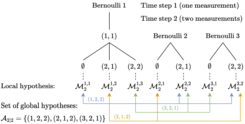
Figure 1: An example of Bernoulli components and hypotheses maintained by a PMBM density of the form (4). A new Bernoulli component is created for each measurement; this results in three Bernoulli components being created in total. At time step 2, the existing Bernoulli component (Bernoulli 1) has three local hypotheses: one for misdetection (marked with $\emptyset$) and two for measurement update (marked with $(t,j)$). Each new Bernoulli component (Bernoulli 2 and 3) has two local hypotheses: one for the case that the measurement is associated with Bernoulli 1 and one for the case that the measurement is used for updating the PPP. The coloured lines represent three global hypotheses, each of which is a choice of one local hypothesis for each Bernoulli component subject to constraint (8).

III-B Trajectory PMBM Filtering

We present the trajectory PMBM filtering recursion, where the trajectory Poisson intensity $\lambda^{u}_{k^{\prime}|k}(\cdot)$ and the single trajectory density $f_{k^{\prime}|k}^{i,a^{i}}(\cdot)$, $i\in\{1,\dots,n_{k^{\prime}|k}\}$, $a^{i}\in\{1,\dots,h^{i}\}$, of each local hypothesis have a mixture representation (cf. (1)),

$$\lambda^{u}_{k^{\prime}|k}\left(X\right) =\sum_{l=1}^{L^{u}_{k^{\prime}|k}}\nu_{k^{\prime}|k}^{u,l}p_{k^{\prime}|k}^{u,l}\left(x_{\beta:\varepsilon}|\beta,\varepsilon\right)\delta_{b^{u,l}_{k^{\prime}|k}}[\beta]\delta_{e^{u,l}_{k^{\prime}|k}}[\varepsilon],$$ (9)

$$f_{k^{\prime}|k}^{i,a^{i}}\left(X\right) =\sum_{l=1}^{L^{i,a^{i}}_{k^{\prime}|k}}\nu_{k^{\prime}|k}^{i,a^{i},l}p_{k^{\prime}|k}^{i,a^{i},l}\left(x_{\beta:\varepsilon}|\beta,\varepsilon\right)\delta_{b^{i,a^{i},l}_{k^{\prime}|k}}[\beta]\delta_{e^{i,a^{i},l}_{k^{\prime}|k}}[\varepsilon],$$ (10)

where the $l$-th component in single-trajectory function $\lambda^{u}_{k^{\prime}|k}(\cdot)$ and $f_{k^{\prime}|k}^{i,a^{i}}(\cdot)$ is characterized by $(\nu_{k^{\prime}|k}^{u,l},p_{k^{\prime}|k}^{u,l}(\cdot),b^{u,l}_{k^{\prime}|k},e^{u,l}_{k^{\prime}|k})$ and $(\nu_{k^{\prime}|k}^{i,a^{i},l},p_{k^{\prime}|k}^{i,a^{i},l}(\cdot),b^{i,a^{i},l}_{k^{\prime}|k},e^{i,a^{i},l}_{k^{\prime}|k})$, respectively.

Since in practice, trajectories that have never been detected and no longer exist at the current time step are generally of little importance, they do not need to be explicitly represented in practical implementations. That is, the PPP of undetected trajectories here only consider alive trajectories with $e^{u,l}_{k^{\prime}|k}=k^{\prime}$, $l\in\{1,\dots,L^{u}_{k^{\prime}|k}\}$ in (9). We also assume that the trajectory Poisson birth intensity $\lambda_{k+1}^{B}(\cdot)$ is of the mixture form (cf. (1))

$$\lambda_{k+1}^{B}(X)=\delta_{k+1}[\beta]\delta_{k+1}[\varepsilon]\sum_{l=1}^{L^{B}}\nu^{B,l}p^{B,l}(x_{\beta:\varepsilon}|\beta,\varepsilon).$$ (11)

In addition, we use $p_{k^{\prime}|k}(x_{t})$ to represent the marginalized object state $x_{t}$ density at time step $t\in\{\beta,\dots,\varepsilon\}$, obtained from $p_{k^{\prime}|k}(x_{\beta:\varepsilon})$.

Proposition 1 (Trajectory PMBM update)

Assume that the predicted density $f_{k|k-1}(\cdot)$ is a PMBM (4) with $\lambda^{u}_{k|k-1}(\cdot)$ and $f^{i,a^{i}}_{k|k-1}(\cdot)$ given by (9) and (10). The filtering density $f_{k|k}(\cdot)$, updated with measurements $\mathbf{z}_{k}$, is also a PMBM (4).

For PPP of undetected trajectories, the updated $l$-th component in (9) is

$$p_{k|k}^{u,l}(x_{\beta:k}|\beta,k) =\frac{\left(1-p^{D}\left(x_{k}\right)\right)p_{k|k-1}^{u,l}(x_{\beta:k}|\beta,k)}{\left\langle 1-p^{D},p^{u,l}_{k|k-1}\right\rangle},$$ (12a)

$$b^{u,l}_{k|k} =b^{u,l}_{k|k-1},\quad e^{u,l}_{k|k}=e^{u,l}_{k|k-1},$$ (12b)

$$\nu_{k|k}^{u,l} =\left\langle 1-p^{D},p^{u,l}_{k|k-1}\right\rangle\nu_{k|k-1}^{u,l}.$$ (12c)

The number of Bernoulli components is $n_{k|k}=n_{k|k-1}+m_{k}$. For Bernoulli components continuing from previous time steps $i\in\{1,\dots,n_{k|k-1}\}$, a local hypothesis is included for each combination of a local hypothesis from a previous time step, and either a misdetection or an update using one of the $m_{k}$ new measurements, such that the number of local hypotheses becomes $h^{i}_{k|k}=h^{i}_{k|k-1}(1+m_{k})$.

A misdetection hypothesis takes into account both the case that the trajectory does not exist and the case that the trajectory exists but ends before current time step $k$. For misdetection hypotheses with $i\in\{1,\dots,n_{k|k-1}\}$, $a^{i}\in\{1,\dots,h^{i}_{k|k-1}\}$:

$$\Phi^{i,a^{i},0}_{k}=\sum_{l=1}^{L^{i,a^{i}}_{k|k-1}}\delta_{k}\left[e^{i,a^{i},l}_{k|k-1}\right]\nu_{k|k-1}^{i,a^{i},l}\left\langle p_{k|k-1}^{i,a^{i},l},p^{D}\right\rangle,$$ (13a)

$$w^{i,a^{i}}_{k|k}=w_{k|k-1}^{i,a^{i}}\left(1-r_{k|k-1}^{i,a^{i}}\Phi^{i,a^{i},0}_{k}\right),$$ (13b)

$$r^{i,a^{i}}_{k|k}=\frac{r^{i,a^{i}}_{k|k-1}\left(1-\Phi^{i,a^{i},0}_{k}\right)}{1-r^{i,a^{i}}_{k|k-1}\Phi^{i,a^{i},0}_{k}},$$ (13c)

$$p_{k|k}^{i,a^{i},l}(x_{\beta:\varepsilon}|\beta,\varepsilon)=\frac{\left(1-p^{D}(x_{k})\right)p_{k|k-1}^{i,a^{i},l}(x_{\beta:\varepsilon}|\beta,\varepsilon)}{\left\langle 1-p^{D},p_{k|k-1}^{i,a^{i},l}\right\rangle},$$ (13d)

$$b^{i,a^{i},l}_{k|k}=b^{i,a^{i},l}_{k|k-1},\quad e^{i,a^{i},l}_{k|k}=e^{i,a^{i},l}_{k|k-1},$$ (13e)

$$\nu^{i,a^{i},l}_{k|k}=\begin{cases}\frac{\nu^{i,a^{i},l}_{k|k-1}}{1-\Phi^{i,a^{i},0}_{k}}&e^{i,a^{i},l}<k\\ \frac{\nu^{i,a^{i},l}_{k|k-1}\left\langle 1-p^{D},p^{i,a^{i},l}_{k|k-1}\right\rangle}{1-\Phi^{i,a^{i},0}_{k}}&e^{i,a^{i},l}=k.\end{cases}$$ (13f)

For hypotheses updating existing Bernoulli components, $i\in\{1,\dots,n_{k|k-1}\}$, $a^{i}=\widetilde{a}^{i}+h^{i}_{k|k-1}j$, $j\in\{1,\dots,m_{k}\}$, i.e. the previous hypothesis $\widetilde{a}^{i}$ is updated with measurement $z_{k}^{j}$:

$$\mathcal{M}_{k}^{i,a^{i}}=\mathcal{M}_{k-1}^{i,\widetilde{a}^{i}}\cup\{(k,j)\},$$ (14a)

$$\Phi_{k}^{i,a^{i},j}=\sum_{l=1}^{L^{i,\widetilde{a}^{i}}_{k|k-1}}\delta_{k}\left[e^{i,\widetilde{a}^{i},l}_{k|k-1}\right]\nu_{k|k-1}^{i,\widetilde{a}^{i},l}\left\langle p_{k|k-1}^{i,\widetilde{a}^{i},l},\ell\left(z_{k}^{j}|\cdot\right)p^{D}\right\rangle,$$ (14b)

$$w^{i,a^{i}}_{k|k}=w^{i,\widetilde{a}^{i}}_{k|k-1}r^{i,\widetilde{a}^{i}}_{k|k-1}\Phi_{k}^{i,a^{i},j},$$ (14c)

$$r^{i,a^{i}}_{k|k}=1,$$ (14d)

$$p^{i,a^{i},l}_{k|k}\left(x_{\beta:\varepsilon}|\beta,\varepsilon\right)=\frac{p^{D}(x_{k})p_{k|k-1}^{i,\widetilde{a}^{i},l}\left(x_{\beta:\varepsilon}|\beta,\varepsilon\right)\ell\left(z_{k}^{j}|x_{k}\right)}{\left\langle p_{k|k-1}^{i,\widetilde{a}^{i},l},\ell\left(z_{k}^{j}|\cdot\right)p^{D}\right\rangle},$$ (14e)

$$b^{i,a^{i},l}_{k|k}=b^{i,a^{i},l}_{k|k-1},\quad e^{i,a^{i},l}_{k|k}=e^{i,a^{i},l}_{k|k-1},$$ (14f)

$$\nu_{k|k}^{i,a^{i},l}=\begin{cases}0&e^{i,\widetilde{a}^{i},l}_{k|k-1}<k\\ \frac{\nu_{k|k-1}^{i,\widetilde{a}^{i},l}\left\langle p_{k|k-1}^{i,\widetilde{a}^{i},l},\ell\left(z_{k}^{j}|\cdot\right)p^{D}\right\rangle}{\Phi_{k}^{i,a^{i},j}}&e^{i,\widetilde{a}^{i},l}_{k|k-1}=k.\end{cases}$$ (14g)

We note that for local hypotheses resulted from measurement update, the trajectory exists and is alive at current time step $k$ with probability one.

Finally, each new Bernoulli component, $i=n_{k|k-1}+j$, $j\in\{1,\dots,m_{k}\}$, is initiated with two local hypotheses ($h^{i}_{k|k}=2$), the first of which covers the case that measurement $z_{k}^{j}$ is associated with another Bernoulli component; the second of which covers the case that measurement $z_{k}^{j}$ is either a false alarm or the first detection of an undetected trajectory:

$$\mathcal{M}_{k}^{i,1}=\emptyset,\quad w_{k|k}^{i,1}=1,\quad r_{k|k}^{i,1}=0,$$ (15a)

$$\mathcal{M}_{k}^{i,2}=\{(k,j)\},\quad L_{k|k}^{i,2}=L_{k|k-1}^{u}$$ (15b)

$$\Phi_{k}^{u,j}=\sum_{l=1}^{L^{u}_{k|k-1}}\nu_{k|k-1}^{u,l}\left\langle p_{k|k-1}^{u,l},\ell\left(z_{k}^{j}|\cdot\right)p^{D}\right\rangle,$$ (15c)

$$w_{k|k}^{i,2}=\lambda^{C}\left(z_{k}^{j}\right)+\Phi_{k}^{u,j},$$ (15d)

$$r_{k|k}^{i,2}=\frac{\Phi_{k}^{u,j}}{w_{k|k}^{i,2}},$$ (15e)

$$p_{k|k}^{i,2,l}\left(x_{\beta:k}|\beta,k\right)=\frac{p^{D}(x_{k})p_{k|k-1}^{u,l}\left(x_{\beta:k}|\beta,k\right)\ell\left(z_{k}^{j}|x_{k}\right)}{\left\langle p_{k|k-1}^{u,l},\ell\left(z_{k}^{j}|\cdot\right)p^{D}\right\rangle},$$ (15f)

$$b^{i,2,l}_{k|k}=b^{u,l}_{k|k-1},\quad e^{i,2,l}_{k|k}=e^{u,l}_{k|k-1},$$ (15g)

$$\nu_{k|k}^{i,2,l}=\frac{\nu_{k|k-1}^{u,l}\left\langle p_{k|k-1}^{u,l},\ell\left(z_{k}^{j}|\cdot\right)p^{D}\right\rangle}{\Phi_{k}^{u,j}}.$$ (15h)

For the first case, the new Bernoulli component has probability of existence equal to zero, and thus its single-trajectory density has no effect. For the second case, the probability of existence $r^{i,2}_{k|k}$ models the relative likelihood of $z_{k}^{j}$ being false alarm or the first detection of an undetected object. We also note that the updated single-trajectory density also captures trajectory information before current time step $k$.

Proposition 2 (Trajectory PMBM prediction)

Assume that the filtering density $f_{k|k}(\cdot)$ is a PMBM (4) with $\lambda^{u}_{k|k}(\cdot)$ and $f^{i,a^{i}}_{k|k}(\cdot)$ given by (9) and (10). The predicted density $f_{k+1|k}(\cdot)$ is also a PMBM (4). For the PPP of undetected trajectories, we have $L^{u}_{k+1|k}=L^{u}_{k|k}+L^{B}$, and

$$p^{u,l}_{k+1|k}\left(x_{\beta:k+1}|\beta,k+1\right)=\frac{p^{S}(x_{k})p^{u,l}_{k|k}\left(x_{\beta:k}|\beta,k\right)g(x_{k+1}|x_{k})}{\left\langle p_{k|k}^{u,l},p^{S}\right\rangle},$$ (16a)

$$b^{u,l}_{k+1|k}=b^{u,l}_{k|k},\quad e^{u,l}_{k+1|k}=e^{u,l}_{k|k}+1,$$ (16b)

$$\nu^{u,l}_{k+1|k}=\nu_{k|k}^{u,l}\left\langle p_{k|k}^{u,l},p^{S}\right\rangle,$$ (16c)

for alive trajectories with $$l\in\{1,\dots,L^{u}_{k|k}\}$$,

$$p^{u,l}_{k+1|k}\left(x_{k+1:k+1}|k+1,k+1\right)=p^{B,l-L^{u}_{k|k}}(x_{k+1}),$$ (16d)

$$b_{k+1|k}^{u,l}=e_{k+1|k}^{u,l}=k+1,$$ (16e)

$$\nu_{k+1|k}^{u,l}=\nu^{B,l-L^{u}_{k|k}},$$ (16f)

for newborn trajectories with $$l\in\{L^{u}_{k|k}+1,\dots,L^{u}_{k+1|k}\}$$.

For Bernoulli components describing detected trajectories, we only need to update mixture components with $e^{i,a^{i},l}_{k|k}=k$ that represent alive trajectories. Specifically, each such mixture component creates two predicted mixture components, the first of which covers the case that the trajectory ends at time $k$,

$$p_{k+1|k}^{i,a^{i},l}\left(x_{\beta:k}|\beta,k\right) =\frac{\left(1-p^{S}(x_{k})\right)p_{k|k}^{i,a^{i},l}\left(x_{\beta:k}|\beta,k\right)}{1-\left\langle p_{k|k}^{i,a^{i},l},p^{S}\right\rangle},$$ (17a)

$$b^{i,a^{i},l}_{k+1|k} =b^{i,a^{i},l}_{k|k},\quad e^{i,a^{i},l}_{k+1|k}=e^{i,a^{i},l}_{k|k},$$ (17b)

$$\nu_{k+1|k}^{i,a^{i},l} =\nu_{k|k}^{i,a^{i},l}\left(1-\left\langle p_{k|k}^{i,a^{i},l},p^{S}\right\rangle\right),$$ (17c)

and the second of which covers the case that the trajectory continues to exist at time step $$k+1$$,

$$p_{k+1|k}^{i,a^{i},l}\left(x_{\beta:k+1}|\beta,k+1\right)=\frac{p^{S}(x_{k})p_{k|k}^{i,a^{i},l}\left(x_{\beta:k}|\beta,k\right)g(x_{k+1}|x_{k})}{\left\langle p_{k|k}^{i,a^{i},l},p^{S}\right\rangle},$$ (17d)

$$b^{i,a^{i},l}_{k+1|k}=b^{i,a^{i},l}_{k|k},\quad e^{i,a^{i},l}_{k+1|k}=e^{i,a^{i},l}_{k|k}+1,$$ (17e)

$$\nu_{k+1|k}^{i,a^{i},l}=\nu_{k|k}^{i,a^{i},l}\left\langle p_{k|k}^{i,a^{i},l},p^{S}\right\rangle.$$ (17f)

We note that the information on whether the trajectory ends, or if it extends by one more time step is compactly encapsulated in the predicted single trajectory density without expanding the global hypothesis space as in [11, 15, 16].

Remark: Proposition 1 and 2 include explicit expressions for predicting and updating single trajectory densities of the form specified by (9) and (10), making them more suitable for practical implementations than the TPMBM filtering recursions in [19] for general single trajectory density functions.

IV Problem Formulation

We aim at estimating the set $\mathbf{X}_{K}$ of all trajectories in the entire time interval of interest through processing the sequence of measurement sets $\mathbf{z}_{1:K}$ in a batch. Formally speaking, our objective is to directly compute the posterior density on set $\mathbf{X}_{K}$ of trajectories $f_{K|K}(\mathbf{X}_{K})$ using batch data $\mathbf{z}_{1:K}$.

Remark: Given the multi-trajectory dynamic and measurement models defined in Section II-B, if the multi-object prior at time step $0$ is a PMBM, then the multi-trajectory posterior $f_{K|K}(\mathbf{X}_{K})$ in the time interval $0:K$ is a PMBM (4).

The main challenge in computing the TPMBM posterior is due to the intractably large number of MB components in the MBM (6), given by the number of global hypotheses $|\mathcal{A}_{K|K}|$. In this paper, we tackle this large scale multidimensional data association problem using MCMC sampling. After obtaining samples of global hypotheses from the stationary distribution, we can only keep those with highest weights, which can be understood as minimizing the $L_{1}$ norm between the MBM and its truncation [32].

Besides finding the global hypotheses with highest weights, we need to compute the Poisson intensity of undetected trajectories $\lambda^{u}_{K|K}(\cdot)$ and the local hypothesis densities $f^{i,a^{i}}_{K|K}(\cdot)$. Specifically, assume that the multi-object prior is $f_{0|0}(\emptyset)=1$, we can obtain $\lambda^{u}_{K|K}(\cdot)$ by recursively applying (16) and (12). The number of Bernoulli components is $n_{K|K}=\sum_{k=1}^{K}m_{k}$. For Bernoulli component $i\in\{\sum_{t=1}^{k-1}m_{t}+1,\dots,\sum_{t=1}^{k}m_{t}\}$ initiated at time step $k$, its number of local hypotheses at time step $K$ is

$$h^{i}_{K|K}=1+\prod_{t=k+1}^{K}(m_{t}+1).$$

Local hypothesis density $f^{i,a^{i}}_{K|K}(\cdot)$, $i\in\{1,\dots,n_{K|K}\}$, $a^{i}\in\{1,\dots,h^{i}_{K|K}\}$, with measurement association history $\mathcal{M}_{K|K}^{i,a^{i}}$ can be computed by recursively applying (13), (14), (15) and (17). We note that for local hypothesis density $f^{i,a^{i}}_{K|K}(\cdot)$ with $|\mathcal{M}_{K}^{i,a^{i}}|\geq 2$, $r_{K}^{i,a^{i}}=1$, and that for $f^{i,a^{i}}_{K|K}(\cdot)$ with $|\mathcal{M}_{K}^{i,a^{i}}|=1$, $r_{K}^{i,a^{i}}\in(0,1)$. This means that we are certain that a Bernoulli component represents an actual trajectory, if and only if it is associated with more than one measurement.

V MCMC Sampling

In this section, we present techniques for efficiently finding global hypotheses with highest weights in the PMBM posterior using MCMC sampling. Two sampling methods are described, one is based on Gibbs sampling, and the other is based on MH sampling. The relation between the proposed MH sampler and the one in [11] is also explained. Finally, we discuss practical considerations in the implementations.

Conceptually, a global data association hypothesis describes a partition of the set $\mathcal{M}_{K}$ of measurement pairs into clusters of measurement pairs associated to the same local hypothesis. Our objective is to run an MCMC chain to sample such data association hypotheses. However, some representations of how we partition the data into clusters can be mathematically inconvenient to work with. Importantly, for point object tracking, we find it convenient to represent data associations from a track-oriented perspective, in contrast to the measurement-oriented data association used in extended object tracking [25], where an object may generate multiple measurement per time scan.

To this end, we introduce an alternative track-oriented data association representation to the local hypothesis measurement association history. Specifically, the correspondence between Bernoulli components and measurements at time step $k$, $k\in\{1,\dots,K\}$, is represented by a vector $\theta_{k}$ of dimension $n_{k|k}$, where $\theta_{k}(i)$ denotes the $i$-th entry of vector $\theta_{k}$. If an existing Bernoulli component $i\in\{1,\dots,n_{k|k-1}\}$ is misdetected or a new Bernoulli component $i\in\{n_{k|k-1}+1,\dots,n_{k|k}\}$ does not exist, then $\theta_{k}(i)=0$. If Bernoulli component $i$ is associated with the $j$-th measurement, then $\theta_{k}(i)=j$.

According to the definition of global hypothesis (8), there are certain constraints on the construction of the track-oriented data association $\theta_{k}$, $k\in\{1,\dots,K\}$:

1. $\theta_{k}(i)\in\{0,1,\dots,m_{k}\},$ $\forall i\in\{1,\dots,n_{k|k-1}\}$.

2. $\theta_{k}(i)\in\{0,j\},$ $\forall i=n_{k|k-1}+j$, and $j\in\{1,\dots,m_{k}\}$.

3. $\theta_{k}(i)\neq\theta_{k}(j)$, $\forall i\neq j,\theta_{k}(i)>0$, and $\theta_{k}(j)>0$.

4. $\forall j\in\{1,\dots,m_{k}\}$, $\exists i\in\{1,\dots,n_{k|k}\}$ such that $\theta_{k}(i)=j$.

5. If $\theta_{k}(i)=0$, where $i\in\{n_{k|k-1}+1,\dots,n_{k|k}\}$, then $\theta_{k+t}(i)=0$, $\forall t\in\{1,\dots,K-k\}$.

Constraint 3) and 4) together mean that each measurement should be assigned to exactly one Bernoulli component. Constraint 5) means that if new Bernoulli component $i$, initiated at time step $k$, does not exist, then it cannot be associated with any measurements at any subsequent time steps. As a direct consequence of constraint 2) and 5), it also holds that

1. If $\exists\theta_{k+t}(i)>0$, where $i\in\{n_{k|k-1}+1,\dots,n_{k|k}\}$ and $t\in\{1,\dots,K-k\}$, then $\theta_{k}(i)=i-n_{k|k-1}$.

Constraint 6) means that if Bernoulli component $i$, initiated at time step $k$, has been associated with any measurements at subsequent time steps, then it must be created by measurement with index $i-n_{k|k-1}$.

The set of all such vectors $\theta_{k}$ at time step $k$ is denoted by $\Theta_{k}$, and the time sequence of $\theta_{k}$ in interval $1:K$ is denoted by $\theta_{1:K}\in\Theta_{1:K}$. With the above constraints 1)–6) in place, each $\theta_{1:k}\in\Theta_{1:k}$ determines a unique partition of $\mathcal{M}_{k}$. We also note that each legal set of local hypothesis measurement association histories $\{\mathcal{M}_{K}^{i,a^{i}}\}$ is a partition of $\mathcal{M}_{K}$. This also means that there is a bijection between $\Theta_{1:k}$ and the set $\mathcal{A}_{k|k}$ of global hypotheses, denoted by $\Lambda_{k}:\Theta_{1:k}\rightarrow\mathcal{A}_{k|k}$. That is, $\Lambda_{k}(\theta_{1:k})=a$ means that $\theta_{1:k}\in\Theta_{1:k}$ corresponds to $a\in\mathcal{A}_{k|k}$, and we can use $\Lambda_{k}^{i}(\theta_{1:k})$ to represent a local hypothesis $a^{i}$ in a global hypothesis $a$. An example of the track-oriented data association representation $\theta_{1:K}$ is illustrated in Fig. 2.

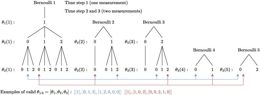
Figure 2: An example of the track-oriented data association sequence $\theta_{1:3}$, where there is one measurement at time step 1 and two measurements at time step 2 and 3. The coloured lines represent two valid $\theta_{1:3}$. For the blue one, Bernoulli $1$ is misdetected at time step 2 and updated by measurement $z_{3}^{1}$ at time step 3; Bernoulli 2 is created by measurement $z_{2}^{1}$ at time step 2 and updated by measurement $z_{3}^{2}$ at time step 3; Bernoulli $3$ is created by measurement $z_{2}^{2}$ at time step 2 and misdetected at time step 3; Bernoulli $4$ and $5$ do not exist. For the red one, Bernoulli 1 is updated by measurement $z_{2}^{1}$ at time step 2 and misdetected at time step 3; Bernoulli 3 is created by measurement $z_{2}^{2}$ at time step 2 and updated by measurement $z_{3}^{2}$ at time step 3; Bernoulli 4 is created by measurement $z_{3}^{1}$ at time step 3; Bernoulli 2 and 5 do not exist. The two global hypotheses $a$ correspond to the blue and red $\theta_{1:3}$ are $(2,4,2,1,1)$ and $(4,1,4,2,1)$, respectively.

Sampling a global hypothesis $a$ from the discrete probability distribution $w^{a}_{K|K}$, $a\in\mathcal{A}_{K|K}$, is equivalent to sampling

$$\theta_{1:K}\sim\pi(\theta_{1:K}) =1_{\Theta_{1:K}}(\theta_{1:K})w_{K|K}^{a}$$

$$\propto 1_{\Theta_{1:K}}(\theta_{1:K})\prod_{i=1}^{n_{K|K}}w_{K|K}^{i,\theta_{1:K}^{i}},$$ (18)

where $\pi(\cdot)$ denotes the pmf of $\theta_{1:K}$, and we define $\theta_{1:K}^{i}\triangleq\Lambda_{K}^{i}(\theta_{1:K})$ for notational brevity. In addition, we also write $\theta_{k}(i:j)\triangleq(\theta_{k}(i),\dots,\theta_{k}(j))$.

V-A Blocked Gibbs Sampling

To sample from (18), we can sequentially draw samples of $\theta_{k}$, $k\in\{1,\dots,K\}$, from the conditional distribution using Gibbs sampling

$$\pi_{k}\left(\theta_{k}|\theta_{1:k-1},\theta_{k+1:K}\right) \propto\pi(\theta_{1:K})$$

$$\propto 1_{\Theta_{1:K}}(\theta_{1:K})\prod_{i=1}^{n_{k|k}}w_{K|K}^{i,\theta_{1:K}^{i}}.$$ (19)

We note that the product over $w_{K|K}^{i,\theta_{1:K}^{i}}$ in (19) goes from $i=1$ to $n_{k|k}$, not $n_{K|K}$ as in (18). This proportionality in (19) holds since, conditioned on $\theta_{k+1:K}$, data association $\theta_{k}(i)$ of Bernoulli component $i\in\{1,\dots,n_{k|k}\}$ at time step $k$ does not depend on Bernoulli components created after time step $k$. To sample $\theta_{k}$ from (19), one possible strategy is to sample one variable $\theta_{k}(i)$ at a time for $i\in\{1,\dots,n_{k|k}\}$ conditioned on $\theta_{1:k-1}$, $\theta_{k+1:K}$, and $\theta_{k}(1:i-1)$, $\theta_{k}(i+1:n_{k|k})$. However, due to the constraints 1)–6) of $\theta_{k}$, it turns out that $\theta_{k}(i)$ is a deterministic function of $\theta_{k}(1:i-1)$ and $\theta_{k}(i+1:n_{k|k})$. This implies that such a sampling algorithm would never change $\theta_{k}$.

According to constraint 2), if at time step $k$ measurement $z_{k}^{j}$ is not associated to an existing Bernoulli component $i\in\{1,\dots,n_{k|k-1}\}$, then it must be used to create new Bernoulli component $n_{k|k-1}+j$ where $j\in\{1,\dots,m_{k}\}$. This means that if at time step $k$ we change the data association $\theta_{k}(i)$ of an existing Bernoulli component $i\in\{1,\dots,n_{k|k-1}\}$ from $j$ to $0$, while fixing the data associations of other existing Bernoulli components, the data association $\theta_{k}(n_{k|k-1}+j)$ of the $j$-th new Bernoulli component must change from $0$ to $j$, and vice versa. In light of this observation, we adopt a blocked Gibbs sampling strategy to jointly sample the data association $\theta_{k}(i)$ of an existing Bernoulli component $i\in\{1,\dots,n_{k|k-1}\}$ and the data associations $\theta_{k}(n_{k|k-1}+1:n_{k|k})$ of all the new Bernoulli components at time step $k$ via

$$\pi_{k,i}^{\theta_{k}(i)} \triangleq\pi_{k}\left(\theta_{k}(i),\theta_{k}(n_{k|k-1}+1:n_{k|k})\right.$$

$$~{}~{}~{}~{}~{}~{}~{}~{}\left.\mid\theta_{1:k-1},\theta_{k}(1:i-1),\theta_{k}(i+1:n_{k|k-1}),\theta_{k+1:K}\right)$$

$$\propto 1_{\Theta_{1:K}}(\theta_{1:K})w_{K|K}^{i,\theta_{1:K}^{i}}\prod_{j=1}^{m_{k}}w_{K|K}^{n_{k|k-1}+j,\theta_{1:K}^{n_{k|k-1}+j}}$$

$$\triangleq 1_{\Theta_{1:K}}(\theta_{1:K})w_{K|K}^{i,\theta_{1:K}^{i}}\Pi_{k,n_{k|k}}^{\theta_{k}(i)},$$ (20)

where we introduce the shorthand notations $\pi_{k,i}^{\theta_{k}(i)}$ and $\Pi_{k,n_{k|k}}^{\theta_{k}(i)}$.

Example: Let us take the red $\theta_{1:3}$ illustrated in Fig. 2 for an example, and say we would like to change the data association $\theta_{3}(3)=2$ of Bernoulli 3 at time step 3 while fixing $\theta_{3}(1)$ and $\theta_{3}(2)$. If we change $\theta_{3}(3)$ from 2 to 0, then we must also change $\theta_{3}(5)$ from 0 to 2. If we change $\theta_{3}(3)$ from 2 to 1, then we must also change $\theta_{3}(4)$ from 1 to 0 and $\theta_{3}(5)$ from 0 to 2. This means that $\theta_{3}(3)$ cannot be changed alone while fixing all the other data associations $\theta_{3}(1:2)$ and $\theta_{3}(4:5)$. However, it is possible to jointly modify the data associations $\theta_{3}(3:5)$. That is, we can change $\theta_{3}(3:5)=[2,1,0]$ to either $[0,1,2]$ or $[1,0,2]$. We also note that the change of $\theta_{3}(4:5)$ is uniquely determined by $\theta_{3}(3)$.

Further, since the data associations $\theta_{k}(n_{k|k-1}+1:n_{k|k})$ of new Bernoulli components are deterministic functions of the data associations $\theta_{k}(1:n_{k|k-1})$ of existing Bernoulli components, it is sufficient to only sample the data association $\theta_{k}(i)$ of existing Bernoulli components for each group of variables $(\theta_{k}(i),\theta_{k}(n_{k|k-1}+1:n_{k|k}))$, $i\in\{1,\dots,n_{k|k-1}\}$. Note that this is also why we only explicitly denoted the dependences of $\pi_{k,i}^{\theta_{k}(i)}$ and $\Pi_{k,n_{k|k}}^{\theta_{k}(i)}$ on $\theta_{k}(i)$ for brevity. Moreover, there is a convenient method to sample $\theta_{k}(i)$ that greatly simplifies the computation of the product of $m_{k}+1$ factors in (20).

The key to simplifying the unnormalized expression in (20) is to note that the ratio between the conditional probabilities of the two cases $\theta_{k}(i)=j$, $j\in\{1,\dots,m_{k}\}$, and $\theta_{k}(i)=0$ has a simple form. Specifically, the product $\Pi_{k,n_{k|k}}^{\theta_{k}(i)}$ over the $m_{k}$ local hypothesis weights in (20) of the two cases only differs in the $j$-th factor, i.e. the local hypothesis weight that measurement $z_{k}^{j}$ initiates a new Bernoulli component, which can take two different values depending on data association $\theta_{k}(n_{k|k-1}+j)$. First, if $\theta_{k}(n_{k|k-1}+j)=0$, which means that measurement $z_{k}^{j}$ is associated with an existing Bernoulli component, the corresponding local hypothesis weight is one (cf. (15a)). Second, if $\theta_{k}(n_{k|k-1}+j)=j$, then measurement $z_{k}^{j}$ is associated to the $j$-th new Bernoulli component at time step $k$. Moreover, for the latter case, if Bernoulli component $n_{k|k-1}+j$ has also been associated with any measurements at subsequent time steps, then, due to constraint 6), we cannot change the data association $\theta_{k}(n_{k|k-1}+j)=j$. That is, in this case we have that $\pi_{k,i}^{\theta_{k}(i)}=0$. Therefore, we only need to focus on the case that Bernoulli component $n_{k|k-1}+j$ is only detected once at time step $k$.

We denote the data association sequence where each measurement initiates a Bernoulli component as $\hat{\theta}_{1:K}$, which, for each time step $k\in\{1,\dots,K\}$, satisfies that $\widehat{\theta}_{k}(n_{k|k-1}+j)=j$, $j\in\{1,\dots,m_{k}\}$, and $\widehat{\theta}_{t}(i)=0$ for $i\in\{1,\dots,n_{k|k-1}\}$ and $t\in\{k+1,\dots,K\}$. According to the above analysis, the ratio between the factors $\Pi_{k,n_{k|k}}^{\theta_{k}(i)}$ of the two cases $\theta_{k}(i)=j$ (denoted as $\Pi_{k,n_{k|k}}^{\theta_{k}(i)=j}$), where $j\in\{1,\dots,m_{k}\}$, and $\theta_{k}(i)=0$ (denoted as $\Pi_{k,n_{k|k}}^{\theta_{k}(i)=0}$) is

$$\frac{\Pi_{k,n_{k|k}}^{\theta_{k}(i)=j}}{\Pi_{k,n_{k|k}}^{\theta_{k}(i)=0}}=\frac{1}{w_{K|K}^{n_{k|k-1}+j,\widehat{\theta}^{n_{k|k-1}+j}_{1:K}}},$$ (21)

where $w_{K|K}^{n_{k|k-1}+j,\widehat{\theta}^{n_{k|k-1}+j}_{1:K}}$ is the weight of local hypothesis that Bernoulli component $n_{k|k-1}+j$ is only detected once at time step $k$. Dividing (20) by $\Pi_{k,n_{k|k}}^{\theta_{k}(i)=0}$ and using (21) yields the following simplified expression of (20):

$$\pi_{k,i}^{\theta_{k}(i)}\propto 1_{\Theta_{1:K}}(\theta_{1:K})\begin{cases}w_{K|K}^{i,\theta_{1:K}^{i}}&\theta_{k}(i)=0\\ \frac{w_{K|K}^{i,\theta_{1:K}^{i}}}{w_{K|K}^{n_{k|k-1}+j,\widehat{\theta}^{n_{k|k-1}+j}_{1:K}}}&\theta_{k}(i)=j.\end{cases}$$ (22)

The simplified expression (22) has intuitive interpretations: 1) the conditional probability $\pi_{k,i}^{\theta_{k}(i)}$ is proportional to the local hypothesis weight $w_{K|K}^{i,\theta_{1:K}^{i}}$; 2) the conditional probability $\pi_{k,i}^{\theta_{k}(i)}$ is divided by the local hypothesis weight $w_{K|K}^{n_{k|k-1}+j,\widehat{\theta}^{n_{k|k-1}+j}_{1:K}}$ when $\theta_{k}(i)=j$ to compensate the case that measurement $z_{k}^{j}$ is not associated to new Bernoulli component $n_{k|k-1}+j$ at time step $k$.

It is computationally efficient to evaluate (22), making sampling $\theta_{k}(i)$ easy. In addition, the weights $w_{K|K}^{n_{k|k-1}+j,\widehat{\theta}^{n_{k|k-1}+j}_{1:K}}$, $j\in\{1,\dots,m_{k}\}$, $k\in\{1,\dots,K\},$ can be pre-computed to avoid repetitive computations. Starting with any valid $\theta_{1:K}$, the Gibbs sampler draws samples of $(\theta_{k}(i),\theta_{k}(n_{k|k-1}+1:n_{k|k}))$ from (22) by iterating $i\in\{1,\dots,n_{k|k-1}\}$, $k\in\{1,\dots,K\}$. The Gibbs sampler is summarized in Algorithm 1, where $\theta^{(\tau)}$ denotes its value at the $\tau$-th sampling iteration. The choice of the initial data associations $\theta^{(0)}$ is described in Section V-C1.

Algorithm 1 Blocked Gibbs multi-scan data association.

0:  Initial data associations $\theta_{1:K}^{(0)}$, number of iterations $T$.

0:  $\{\theta_{1:K}^{(\tau)}:\tau=1,\dots,T\}$.

1:  for $\tau=1$ to $T$ do

2:     for $k=1$ to $K$ do

3:        for $i=1$ to $n_{k|k-1}$ do

4:           Sample $(\theta_{k}^{(\tau)}(i),\theta_{k}^{(\tau)}(n_{k|k-1}+1:n_{k|k}))$ via (22).

5:        end for

6:     end for

7:  end for

Remark: It is possible to move from any $\theta_{1:K}\in\Theta_{1:K}$ to any other $\widetilde{\theta}_{1:K}\in\Theta_{1:K}$ in finite steps. This means that the Markov chain of $\theta_{1:K}$ is irreducible, which is a sufficient condition for the convergence of Gibbs sampler on discrete variables [33].

V-B Metropolis-Hastings Sampling

The fast mixing of the Markov chain is essential to obtain an efficient MCMC sampling algorithm [34]. In the above-described method using blocked Gibbs sampling, we change the data associations of an existing Bernoulli component and all the new Bernoulli components at a single time step at a time. This, however, may lead to poor mixing of the Markov chain if hypotheses become highly correlated across time and objects, e.g. in scenarios with closely-spaced objects. Moreover, due to constraint 5) of $\theta_{1:K}$, changing the assignment of measurements that have been used to initiate Bernoulli components may take many intermediate steps. A more appealing strategy is to use MH sampling to simultaneously change the measurement association of multiple Bernoulli components across multiple time steps.

To sample from (18) using MH sampling, we first pick a valid data association ${\theta}_{1:K}^{(0)}$ as the initial state of the Markov chain. Then at the $\tau$-th iteration, we draw a data association ${\theta}_{1:K}$ from a proposal distribution $q(\cdot|{\theta}_{1:K}^{(\tau-1)})$, which specifies the probability of proposing ${\theta}_{1:K}$ conditioned on ${\theta}_{1:K}^{(\tau-1)}$. The proposed data association ${\theta}_{1:K}$ is accepted with probability

$$A\left({\theta}_{1:K},{\theta}_{1:K}^{(\tau-1)}\right)=\min\left(1,\frac{\pi\left({\theta}_{1:K}\right)q\left({\theta}_{1:K}^{(\tau-1)}|{\theta}_{1:K}\right)}{\pi\left({\theta}_{1:K}^{(\tau-1)}\right)q\left({\theta}_{1:K}|{\theta}_{1:K}^{(\tau-1)}\right)}\right).$$ (23)

If ${\theta}_{1:K}$ is accepted, we set ${\theta}_{1:K}^{(\tau)}={\theta}_{1:K}$, otherwise ${\theta}_{1:K}^{(\tau)}={\theta}_{1:K}^{(\tau-1)}$. Given enough number of iterations $T$, ${\theta}_{1:K}$ can be regarded as a sample from the stationary distribution (18).

To develop efficient MH sampling algorithms, it is important to construct proposal distributions $q(\cdot|\cdot)$ that can well explore the data association space and are straightforward to evaluate. The proposal distributions for batch TPMBM implementation using MH sampling consist of four moves: 1) track update move, 2) merge/split move, and 3) track switch move, see Fig. 3 for an illustration. For convenience, we index each type of move by an integer $c$, with $c=1$ for the track update move, $c=2$ for the merge move, $c=3$ for the split move, and finally $c=4$ for the track switch move.

Each move is chosen randomly from a category distribution $p(c)$, which should be constructed according to the MB density conditioned on ${\theta}_{1:K}$ and the tracking scenario of interest. For instance, in challenging MOT scenarios with closely-spaced objects, we could increase the probability of performing track switch move $p(c=4)$. The proposal distribution $q(\cdot|\cdot)$ is constructed from a mixture of the form [35, Eq. (11.42)]

$$q\left(\widetilde{\theta}_{1:K}|\theta_{1:K}\right)=\sum_{c=1}^{4}p(c)q_{c}\left(\widetilde{\theta}_{1:K}|\theta_{1:K}\right),$$ (24)

where auxiliary variable $c$ determines the distribution $q_{c}(\cdot|\cdot)$ to be sampled and $q_{c}(\widetilde{\theta}_{1:K}|\cdot)$ takes non-zero values only if $\widetilde{\theta}_{1:K}$ is obtained by taking the corresponding move $c$. The use of this composite proposal distribution (24) is known as reversible jump MCMC in the literature [36].

We proceed to describe each proposal move conditioned on a valid data association $\theta_{1:K}$ in detail.

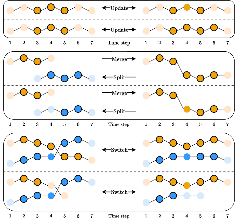
Figure 3: Examples of four proposal moves. Each proposal move is illustrated with two examples, separated using a dash line. The object state sequences are represented using chained circles. Circles with/without borderline represent measurement detection/misdetection. In addition, circles in light orange/blue represent object states with existence uncertainty. For instance, the trajectory in the top left corner has a maximum length of 7. It is first detected at time step 3 and last detected at time step 5, but it may start at time step 1, 2, or 3 and end at time step 5, 6, or 7.

V-B1 Track update move

For a track update move, we first sample a Bernoulli component $i$ uniformly at random (u.a.r.) from the index set of Bernoulli components that are associated with at least two measurements

$$\mathbb{I}_{r=1}=\left\{i\in\{1,\dots,n_{K|K}\}:r_{K|K}^{i,\theta^{i}_{1:K}}=1\right\},$$ (25)

where $r_{K|K}^{i,\theta^{i}_{1:K}}$ is the probability of existence of the $\theta_{1:K}^{i}$-th local hypothesis of the $i$-th Bernoulli component that is included in global hypothesis $\Lambda_{K}(\theta_{1:K})$.

For the selected Bernoulli component $i$, we denote its first detected time step as

$$t_{\text{first}}^{i}=\min\left(\left\{k\in\{1,\dots,K\}:\exists\theta_{k}(i)>0\right\}\right),$$ (26)

and we denote its maximum end time as

$$t_{\text{end}}^{i}=\max\left(\left\{e_{K|K}^{i,\theta_{1:K}^{i},l}\right\}_{l=1}^{L_{K|K}^{i,\theta_{1:K}^{i}}}\right),$$ (27)

where $e_{K|K}^{i,\theta_{1:K}^{i},l}$ is the trajectory end time of the $l$-th component in the single-trajectory density of the $\theta_{1:K}^{i}$-th local hypothesis of the $i$-th Bernoulli component. Then we sample a time step $t$ u.a.r. from the time interval $t_{\text{first}}^{i}+1:t_{\text{end}}^{i}$ and draw a random sample of $({\theta}_{t}(i),{\theta}_{t}(n_{t|t-1}+1:n_{t|t}))$ from (22) with $k=t$ via blocked Gibbs sampling described in Section V-A.

Under the above setting, the proposal distribution is

$$q_{1}\left(\widetilde{\theta}_{1:K}|{\theta}_{1:K}\right)=\frac{\pi_{t,i}^{\widetilde{\theta}_{t}(i)}}{|\mathbb{I}_{r=1}|\left(t_{\text{end}}^{i}-t_{\text{first}}^{i}\right)}.$$ (28)

The Gibbs sampling procedure can be regarded as a particular instance of the MH algorithm where the acceptance probability is one [35, Eq. (11.49)]. Thus, the MH sampling steps for track update moves are always accepted.

Remark: When $p(c=1)=1$, the presented MH sampler reduces to a Gibbs sampler, where variables $({\theta}_{t}(i),{\theta}_{t}(n_{t|t-1}+1:n_{t|t}))$ to be updated at each step are chosen at random instead of by cycling $i,t$ in some particular order.

V-B2 Merge/split move

For a merge move, we first sample a Bernoulli component $i$ u.a.r. from the index set of Bernoulli components that are associated with at least one measurement

$$\mathbb{I}_{r>0}=\left\{i\in\{1,\dots,n_{K|K}\}:r_{K|K}^{i,\theta^{i}_{1:K}}>0\right\}.$$ (29)

For the selected Bernoulli component $i$, we denote its last detected time step as

$$t_{\text{last}}^{i}=\max\left(\left\{k\in\{1,\dots,K\}:\exists\theta_{k}(i)>0\right\}\right).$$ (30)

Then we sample a trajectory Bernoulli component $i^{\prime}$ u.a.r. from the index set of Bernoulli components that are either initiated after time step $t_{\text{last}}^{i}$ or last detected before time step $t_{\text{first}}^{i}$

$$\mathbb{I}_{t^{i}}=\left\{i^{\prime}\in\{1,\dots,n_{K|K}\}:t^{i^{\prime}}_{\text{first}}>t_{\text{last}}^{i}~{}\text{or}~{}t^{i^{\prime}}_{\text{last}}<t_{\text{first}}^{i}\right\}.$$ (31)

In a merge move, we first let $\widetilde{\theta}_{1:K}=\theta_{1:K}$, and then

• If $t^{i^{\prime}}_{\text{first}}>t_{\text{last}}^{i}$, we set $\widetilde{\theta}_{k}(i)=\theta_{k}(i^{\prime})$ and $\widetilde{\theta}_{k}(i^{\prime})=0$ for $k\in\{t^{i^{\prime}}_{\text{first}},\dots,t^{i^{\prime}}_{\text{last}}\}$.

• If $t^{i^{\prime}}_{\text{last}}<t_{\text{first}}^{i}$, we set $\widetilde{\theta}_{k}(i^{\prime})=\theta_{k}(i)$ and $\widetilde{\theta}_{k}(i)=0$ for $k\in\{t^{i}_{\text{first}},\dots,t^{i}_{\text{last}}\}$.

After merging, one of the two Bernoulli components is not associated with any measurements, and this Bernoulli component has local hypothesis weight one and probability of existence zero (cf. (15a)).

The reverse of a merge move is a split move. For a split move, we first sample a Bernoulli component $i$ u.a.r. from $\mathbb{I}_{r=1}$ (25). Then we sample a time step $t$ u.a.r. from the set of time steps that Bernoulli component $i$ is associated with a measurement (except for time step $t^{i}_{\text{first}}$)

$$\mathbb{I}_{\theta_{k}(i)}=\left\{k\in\{t^{i}_{\text{first}}+1,\dots,t^{i}_{\text{last}}\}:\exists\theta_{k}(i)>0\right\}.$$ (32)

In a split move, we first let $\widetilde{\theta}_{1:K}=\theta_{1:K}$, and then we set $\theta_{k}(i)=0$ and $\widetilde{\theta}_{k}(i^{\prime})=\theta_{k}(i)$ where $i^{\prime}=\sum_{k^{\prime}=1}^{t-1}m_{k^{\prime}}+\theta_{t}(i)$ for $k\in\{t,\dots,t^{i}_{\text{last}}\}$. That is, after splitting, Bernoulli component $i$ is not associated with any measurements since time step $t$, and Bernoulli component $i^{\prime}$ initiated by measurement $z_{t}^{\theta_{t}(i)}$ at time step $t$ inherits the measurement association of Bernoulli component $i$ after time step $t$.

The probability of proposing a merge move $q_{2}(\cdot|\cdot)$ or a split move $q_{3}(\cdot|\cdot)$ is easy to compute since both moves are sampled u.a.r. Specifically, we have

$$q_{2}\left(\widetilde{\theta}_{1:K}|{\theta}_{1:K}\right) =\frac{1}{|\mathbb{I}_{r>0}||\mathbb{I}_{t^{i}}|},$$ (33)

$$q_{3}\left(\widetilde{\theta}_{1:K}|{\theta}_{1:K}\right) =\frac{1}{|\mathbb{I}_{r=1}||\mathbb{I}_{\theta_{k}(i)}|}.$$ (34)

To evaluate the acceptance probability (23), we also need to compute the ratio of the two data association probabilities $\pi(\cdot)$ after and before the move. For the merge move, this ratio is

$$\frac{\pi\left(\widetilde{\theta}_{1:K}\right)}{\pi(\theta_{1:K})}=\begin{cases}\frac{w_{K|K}^{i,\widetilde{\theta}_{1:K}^{i}}}{w_{K|K}^{i,\theta_{1:K}^{i}}w_{K|K}^{i^{\prime},\theta_{1:K}^{i^{\prime}}}}&t^{i^{\prime}}_{\text{first}}>t_{\text{last}}^{i}\\ \frac{w_{K|K}^{i^{\prime},\widetilde{\theta}_{1:K}^{i^{\prime}}}}{w_{K|K}^{i,\theta_{1:K}^{i}}w_{K|K}^{i^{\prime},\theta_{1:K}^{i^{\prime}}}}&t^{i^{\prime}}_{\text{last}}<t_{\text{first}}^{i}.\end{cases}$$ (35)

As for the split move, the ratio is given by

$$\frac{\pi\left(\widetilde{\theta}_{1:K}\right)}{\pi(\theta_{1:K})}=\frac{w_{K|K}^{i,\widetilde{\theta}_{1:K}^{i}}w_{K|K}^{i^{\prime},\widetilde{\theta}_{1:K}^{i^{\prime}}}}{w_{K|K}^{i,{\theta}_{1:K}^{i}}}.$$ (36)

V-B3 Track switch move

For a track switch move, we first sample two Bernoulli components $i$, $i^{\prime}$ ($i\neq i^{\prime}$) u.a.r. from $\mathbb{I}_{r=1}$ (25). Then we sample a time step $t$ u.a.r. from the time interval

$$\max\left(t^{i}_{\text{first}},t^{i^{\prime}}_{\text{first}}\right)+1:\max\left(t^{i}_{\text{last}},t^{i^{\prime}}_{\text{last}}\right).$$

To perform a track switch move, we first let $\widetilde{\theta}_{1:K}=\theta_{1:K}$, and then we swap the measurement associations $\widetilde{\theta}_{k}(i)$ and $\widetilde{\theta}_{k}(i^{\prime})$ for $k\in\{t,\dots,\max(t^{i}_{\text{last}},t^{i^{\prime}}_{\text{last}})\}$. Since the track switch move is self-reversible, it holds that $q_{4}(\widetilde{\theta}_{1:K}|\theta_{1:K})=q_{4}(\theta_{1:K}|\widetilde{\theta}_{1:K})$. The ratio of the data association weights after and before the move is

$$\frac{\pi\left(\widetilde{\theta}_{1:K}\right)}{\pi(\theta_{1:K})}=\frac{w_{K|K}^{i,\widetilde{\theta}_{1:K}^{i}}w_{K|K}^{i^{\prime},\widetilde{\theta}_{1:K}^{i^{\prime}}}}{w_{K|K}^{i,{\theta}_{1:K}^{i}}w_{K|K}^{i^{\prime},{\theta}_{1:K}^{i^{\prime}}}}.$$ (37)

The choice of these four moves can be justified as follows. For changing the measurement association history of a single Bernoulli component, we may either change the measurement association at a single time step, or split the measurement association history into two parts. For simultaneously changing the measurement association history of two Bernoulli components, we may swap the measurement associations at a single time step, or merge the two measurement association histories. The MH sampler is summarized in Algorithm 2.

Algorithm 2 Metropolis-Hastings multi-scan data association.

0:  Initial data associations $\theta_{1:K}^{(0)}$, number of iterations $T$.

0:  $\{\theta_{1:K}^{(\tau)}:\tau=1,\dots,T\}$.

1:  for $\tau=1$ to $T$ do

2:     Sample $c\sim p(c)$.

3:     if $c==1$ (track update move) then

4:        Sample $\theta_{1:K}\sim q_{1}(\widetilde{\theta}_{1:K}|\theta_{1:K})$.

5:        $A({\theta}_{1:K},{\theta}_{1:K}^{(\tau-1)})=1$.

6:     else if $c==2$ (merge move) then

7:        Sample $\theta_{1:K}\sim q_{2}(\widetilde{\theta}_{1:K}|\theta_{1:K})$.

8:        Compute $A({\theta}_{1:K},{\theta}_{1:K}^{(\tau-1)})$ using (33), (34) and (35).

9:     else if $c==3$ (split move) then

10:        Sample $\theta_{1:K}\sim q_{3}(\widetilde{\theta}_{1:K}|\theta_{1:K})$.

11:        Compute $A({\theta}_{1:K},{\theta}_{1:K}^{(\tau-1)})$ using (33), (34) and (36).

12:     else if $c==4$ (track switch move) then

13:        Sample $\theta_{1:K}\sim q_{4}(\widetilde{\theta}_{1:K}|\theta_{1:K})$.

14:        Compute $A({\theta}_{1:K},{\theta}_{1:K}^{(\tau-1)})$ using (37).

15:     end if

16:     Sample $u\sim\text{Uniform}([0,1])$.

17:     if $u<A({\theta}_{1:K},{\theta}_{1:K}^{(\tau-1)})$ then

18:        $\theta_{1:K}^{(\tau)}={\theta}_{1:K}$.

19:     else

20:        $\theta_{1:K}^{(\tau)}=\theta_{1:K}^{(\tau-1)}$.

21:     end if

22:  end for

There are several important differences between the proposal distribution presented here and the proposal distributions in [11]. First, there are no birth/death and extension/reduction moves, since uncertainties on trajectory existence and start/end times are captured via single trajectory densities. That is, these events are never sampled in TPMBM; instead they are analytically marginalized out given a global hypothesis. Second, the proposed track update moves using Gibbs sampling are always accepted, allowing faster convergence of the Markov chain. Third, the track switch move presented here considers more cases, also enabling the swap of measurement association sequence and consecutive misdetections, see the illustration at the bottom of Fig. 3 (below the dash line) for an example. This is not possible for the track switch move in the MCMC implementations presented in [11, 15], which only covers the case of swapping measurement associations, as illustrated by the other example at the bottom of Fig. 3 (above the dash line). Lastly, the data association space does not need to be constrained by incorporating domain-specific knowledge, such as maximum object speed or minimum track length.

Remark: To show that the presented MH sampler converges, it is sufficient to show that the proposal distribution (24) is irreducible and aperiodic [33]. Since it is possible to move from any $\theta_{1:K}\in\Theta_{1:K}$ to any other $\widetilde{\theta}_{1:K}\in\Theta_{1:K}$ in finite steps via the track update moves, the proposal distribution (24) is irreducible. In addition, it is trivial to see that there is always a positive probability that $\theta_{1:K}^{(\tau)}=\theta_{1:K}^{(\tau-1)}$ (in the track update moves), so the proposal distribution (24) is also aperiodic.

V-C Practical Considerations

V-C1 Initialization of the Markov Chain

The above-described MCMC sampling methods can be initialized with any valid data associations $\theta_{1:K}$. A simple initialization choice is by setting $\theta_{k}(n_{k|k-1}+j)=j$ for $j\in\{1,\dots,m_{k}\}$ and all other $\theta_{k}(i)$ to zero for $k\in\{1,\dots,K\}$, which corresponds to the case that each measurement initiates a new Bernoulli component. Better initial data associations $\theta_{1:K}^{(0)}$ can be obtained by running a PMBM filter or a PMB filter with the global nearest neighbour data association.

V-C2 Approximations

The presented MCMC sampling methods can be made more computationally efficient by 1) reducing the data association space, and 2) simplifying the computation of local hypothesis densities and weights.

First, we use gating to remove unlikely measurement associations. Second, for local hypotheses corresponding to newly detected trajectories at time step $k$, we set $r^{i,a^{i}}_{k|k}=0$ if $r^{i,a^{i}}_{k|k}$ is less than a threshold; these local hypotheses do not need to be predicted or updated in subsequent time steps. Third, we prune mixture components in the single trajectory density of local hypotheses with small weights, which amounts to truncating the pmf of trajectory start and end times. After pruning, if the probability that a Bernoulli component that was once detected is alive at a certain time step becomes zero, it does not need to be predicted or updated in subsequent time steps. We also prune mixture components in the PPP intensity of undetected trajectories with small weights.

In addition, to compute the weights of local hypotheses after changing the data associations in MCMC sampling, we need to run the Bernoulli prediction and update equations for the new data association sequence. Instead of computing the smoothed object state densities in each sampling iteration, we use $L$-scan approximation [18] with $L=1$. Under this setting, object states at each time step are considered independent and only the latest object state (if the trajectory is alive) is updated at each time step.

V-C3 Estimation

From the MCMC sampling results, we find unique data association samples and their corresponding global hypotheses. Since all distinct global hypotheses will reduce the $L_{1}$ norm error in truncation [32, Sec. V-D], burn-in time and correlation between consecutive samples are not relevant when approximating the TPMBM posterior. To report a reasonable set of trajectories estimate, we first identify a global hypothesis using, e.g. any of the three estimators described in [31]. Then for each local hypothesis, we find the maximum a posteriori estimates of the trajectory start and end time steps. Finally, we apply backward smoothing to the object state filtering densities to obtain smoothed trajectory estimates.

VI Simulations and Results

In this section, we compare the trajectory estimation performance of the following multi-object trackers with their linear Gaussian implementations:

1. TPMBM filter using Murty’s algorithm [19], referred to as TPMBM-M.

2. TPMBM filter using dual decomposition [22], referred to as TPMBM-DD.

3. Batch TPMBM filter using Gibbs sampling, referred to as B-TPMBM-G.

4. Batch TPMBM filter using MH sampling, referred to as B-TPMBM-MH.

5. Labelled trajectory $\text{MBM}_{01}$ filter with partial smoothing [38] using Murty’s algorithm, referred to as T$\text{MBM}_{01}$-M.

6. Batch labelled trajectory $\text{MBM}_{01}$ filter using multi-scan Gibbs sampling [16], referred to as B-T$\text{MBM}_{01}$-G.

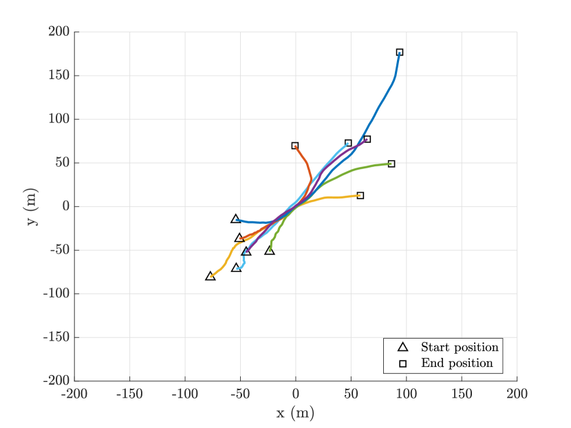
Figure 4: True trajectories of the simulated scenario, which give rise to a difficult data association problem. The start and end positions of trajectories are marked by triangle and square, respectively. There are six objects. They are born at time step 1, 1, 11, 11, 21, and 21, and die at time step 61, 61, 71, 71, 81, and 81, respectively.

Both TPMBM-M and TPMBM-DD are implemented in the Gaussian information form [19] that enables smoothing-while-filtering. For all the other implementations, we apply Rauch-Tung-Striebel smoothing to the object state filtering densities conditioned on the mostly likely global hypothesis to extract smoothed trajectory estimates at the final time step.

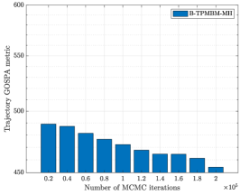
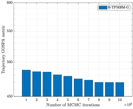
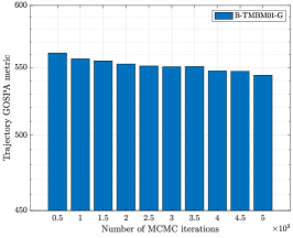
Figure 5: Trajectory GOSPA metric error versus the number of MCMC sampling iterations for B-TPMBM-MH, B-TPMBM-G, and $\text{B-TMBM}_{01}$. Note that the $x$-axis in the three figures has different scales.

In simple scenarios where objects are well spaced, or only a few objects are closely spaced for a limited time steps, the data association uncertainty is low and different implementations present similar tracking performance. For more complex scenarios with higher data association uncertainty, the tracking performance difference among different implementations start to reveal, and it would increase with the number of objects. To this end, we consider a challenging two-dimensional scenario with 81-time steps, where six initially well-separated objects move in close proximity to each other and thereafter separate, in the area $[-200~{}\text{m},200~{}\text{m}]\times[-200~{}\text{m},200~{}\text{m}]$. The true trajectories of the simulated scenario are illustrated in Fig. 4. Each object survives to the next time step with probability $p^{S}=0.98$, and each survived object is moving according to a constant velocity motion model $g(x_{k+1}|x_{k})=\mathcal{N}(Fx_{k},Q)$ with state transition matrix $F$ and motion noise covariance $Q$:

$$F=I_{2}\otimes\begin{bmatrix}1&T_{s}\\ 0&1\end{bmatrix},\quad Q=0.01I_{2}\otimes\begin{bmatrix}T_{s}^{3}/2&T_{s}^{2}/2\\ T_{s}^{2}/2&T_{s}\end{bmatrix},$$

where $T_{s}=1~{}\text{s}$ is the sampling period, $I_{2}$ is an identity matrix and $\otimes$ denotes the Kronecker product. Each object is detected with probability $p^{D}=0.7$, and detected object generates a measurement according to a linear and Gaussian measurement model $\ell(z|x)=\mathcal{N}(Hx,R)$ with observation matrix $H$ and measurement noise covariance $R$:

$$H=I_{2}\otimes\begin{bmatrix}1&0\end{bmatrix},\quad R=I_{2}.$$

The clutter is uniformly distributed in the tracking area with Poisson rate $\lambda^{C}=30$.

For TPMBM implementations, the Poisson birth intensity is a Gaussian mixture with six components, each covering a birth location. For each Gaussian component, its mean is given by its corresponding true object birth state rounded to the nearest integer, with weight $0.01$ and covariance $4I_{2}$. For T$\text{MBM}_{01}$-M and B-T$\text{MBM}_{01}$-G, the MB birth also contains six Bernoulli components, with the same probability hypothesis density as the PPP birth.

All the implementations use ellipsoidal gating with a gating size of probability 0.999 to remove unlikely local hypotheses. For TPMBM implementations, we remove Gaussian components in the Poisson intensity with weight smaller than $10^{-4}$ and also truncate the pmfs of the trajectory birth and end times with probability smaller than $10^{-2}$ and $10^{-4}$, respectively. For online implementations TPMBM-M and TPMBM-DD, we also prune Bernoulli components with probability of existence smaller than $10^{-4}$. For both TPMBM-M and T$\text{MBM}_{01}$-M, the maximum number of global hypotheses is $10^{4}$, and hypotheses with a weight smaller than $10^{-5}$ are pruned. For TPMBM-DD, the sliding window has length $7$ in solving the multi-scan data association.

For batch TPMBM, the Markov chain is initialized using the data association reported by the most likely global hypothesis, obtained by running a TPMBM-M with maximum number of global hypotheses $10^{3}$ and global hypothesis weight pruning threshold $10^{-4}$. In B-T$\text{MBM}_{01}$-G, the Markov chain is instead initialized using T$\text{MBM}_{01}$-M with the same parameter setting. For all the implementations, trajectory estimates are extracted from Bernoulli components with probability of existence $r=1$ included in the most likely global hypothesis (MB component). The multi-trajectory estimation performance is evaluated using the trajectory generalized optimal sub-pattern assignment (GOSPA) metric [39] with order 1, cut-off distance 10, and track switch penalty 2, see Appendix A in the Supplementary Material for its definition. The trajectory GOSPA metric can be decomposed into costs due to state estimation errors, missed and false detections, as well as track switches.

All the simulation results are obtained through 100 Monte Carlo runs. For the proposal distributions used in B-TPMBM-MH, we have tried different settings, all with $2\times 10^{5}$ MCMC sampling iterations, and found that the setting with high track switching probability yielded the best performance, see Table I for an ablation study. This observation is aligned with the intuition that in scenarios with objects moving close to each other, for fast mixing of the Markov chain, it is more efficient to swap the associations of Bernoulli components instead of updating the association of one Bernoulli component at a time. In addition, it is computationally more efficient to perform a track switch move than a track update move.

The total number of sampling iterations used in B-TPMBM-MH, B-TPMBM-G and B-T$\text{MBM}_{01}$-G are $2\times 10^{5}$, $10^{3}$ and $5\times 10^{3}$, respectively. Under this setting, the average runtime for these three implementations is $769~{}\text{s}$, $1241~{}\text{s}$ and $1354~{}\text{s}$, respectively. To empirically study the convergence speed of the different MCMC implementations, Fig. 5 shows how the average trajectory GOSPA error asymptotically decreases with the number of sampling iterations. Together with the average runtime, it is not difficult to see that B-TPMBM-G consistently outperforms $\text{B-TMBM}_{01}$-G in terms of runtime and trajectory GOSPA. It is also worth noting that B-TPMBM-MH is able to perform on par with B-TPMBM-G using about half of its total sampling iterations (and about one-fourth of its runtime). This verifies that MH sampling with the proposal distributions described in Section V-B converges to the stationary distribution much faster than Gibbs sampling with a similar running time.

Figure 6: Trajectory GOSPA errors versus time. B-TPMBM-MH has the best overall performance.

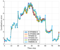
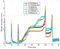
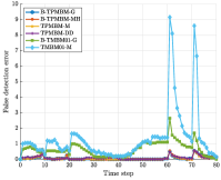
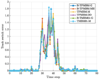
Figure 7: Decomposition of trajectory GOSPA error versus time. The four figures from left to right, respectively, present the localization error, missed detection error, false detection error, and track switch error.

To further analyze the performance of different implementations, the trajectory GOSPA errors and their decompositions over time are shown in Fig. 6 and Fig. 7, respectively. The numerical values of these average trajectory GOSPA errors, together with the average runtime, are presented in Table II. In Fig. 7, the localization error measures the total localization errors for all the detected objects, and it varies with the number of detected objects. The two figures showing the missed and false detection errors reflect the mismatch between the true number of objects and the estimated number of objects. The peaks in these curves correspond to the time steps when new objects are born or existing objects die, or objects move in proximity. In these cases, it is more difficult to detect and localize the objects. Finally, the peaks in the curves showing the track switch error correspond to the time steps when objects moving in proximity. In these cases, it is difficult to distinguish the case where objects are moving separately from the case where objects are moving cross each other, resulting in higher track switch errors.

From Fig. 6, we can observe that on the whole B-TPMBM-MH presents the best trajectory estimation performance, especially fewer misdetections when objects are closely spaced. B-TPMBM-G has the second-best performance, outperforming TPMBM-M and TPMBM-DD by a margin. Also, $\text{B-TMBM}_{01}$-G outperforms T$\text{MBM}_{01}$-M by solving a multi-scan data association problem in a batch. Further, it is interesting to note that, albeit being a batch method, $\text{B-TMBM}_{01}$-G presents worse estimation performance than TPMBM-M and T-PMBM-DD, mainly by showing larger false detection errors when objects die. This is because Bernoulli components in $\text{B-TMBM}_{01}$-G have deterministic existence, which results in an exponential increase of global hypotheses in the prediction step, making it slower for MCMC sampling to explore the data association space. This result highlights the fact that TPMBM has a more efficient hypothesis structure, where object death events are captured in single-trajectory density via the pmf of trajectory end times.

In terms of the trade-off between computational complexity and estimation performance, TPMBM-M mainly depends on the maximum number of global hypotheses allowed in filtering recursion; TPMBM-DD mainly depends on the sliding window length; and B-TPMBM-G and B-TPMBM-MH mainly depend on the number of sampling iterations. The estimation performance of all the implementations could be further improved by increasing their computational budget. However, empirical results show that the performance gain from doing so is limited for online TPMBM implementations. In particular, we did not observe any performance improvement of TPMBM-DD by further increasing its sliding window length. As for TPMBM-M, although it is an online implementation, its runtime under the current setting is already comparable to B-TPMBM-MH. These analyses further highlight the importance of developing batch MOT implementations, which can break the bottleneck of the tracking performance of online implementations.

TABLE I: Performance of B-TPMBM-MH under different settings of the proposal distribution

Trajectory GOSPA Runtime (s) High track switch probability $p(c=4)=1/2,p(c=1,2,3)=1/6$ 454.1 769 Medium track switch probability $p(c=1,4)=1/3,p(c=2,3)=1/6$ 455.0 991 Low track switch probability $p(c=1)=1/2,p(c=2,3,4)=1/6$ 460.3 1201

TABLE II: Trajectory GOSPA metric, its decomposition and runtime

Total Localization Missed False Switch Runtime (s) TPMBM-M 477.7 341.2 116.5 4.6 15.5 613 TPMBM-DD 483.5 348.5 111.5 6.7 16.9 190 B-TPMBM-G 469.7 345.2 103.2 6.0 15.4 1241 B-TPMBM-MH 454.1 349.8 82.8 6.2 15.4 769 T$\text{MBM}_{01}$-M 597.0 358.3 115.4 107.1 16.2 410 $\text{B-TMBM}_{01}$-G 541.5 349.5 123.1 52.3 16.2 1354

VII Conclusions and Future Work

In this paper, we have presented two batch implementations of the TPMBM filter using Gibbs sampling and MH sampling, respectively. The simulation results show that the implementation using the MH algorithm has superior trajectory estimation performance compared to several state-of-the-art algorithms. This result is attributed to the efficient hypothesis structure of TPMBM, the trajectory density representation, and the careful design of the proposal distributions in MH sampling.

An interesting follow-up work is to develop batch TPMBM implementations for extended object tracking. It would be also interesting to explore more advanced MCMC techniques [34] for sampling the data associations. One promising sampling strategy is the use of multiple try Metropolis algorithm [40], where multiple samples are drawn from the proposal distribution at each iteration. Then, one of them is selected as a candidate for the next state according to some suitable weights. To adapt this idea to sample data associations, one may simultaneously consider track update move, merge/split move and track switch move at each iteration, fostering the exploration of the data association space.

Supplementary Materials

Appendix A Trajectory GOSPA Metric

In this appendix, we present the linear programming implementation of the trajectory GOSPA metric [39, Proposition 2] used to evaluate the multi-trajectory estimation performance in Section VI.

For $1\leq p<\infty$, cut-off distance $c>0$, track switching cost $\gamma>0$ and a base metric $d_{b}(\cdot,\cdot)$ in the single object space $\mathbb{R}^{n_{x}}$, the trajectory GOSPA metric between two sets $\mathbf{X}$ and $\mathbf{Y}$ of trajectories in time interval $1,\dots,K$ is given by

$$\bar{d}_{p}^{c,\gamma}(\mathbf{X},\mathbf{Y})=\underset{\begin{subarray}{c}W^{k}\\ k=1,\dots,K\end{subarray}}{\min}\left(\sum_{k=1}^{K}\text{tr}\left[\left(D^{k}_{\mathbf{X},\mathbf{Y}}\right)^{T}W^{k}\right]\right.\\ +\left.\frac{\gamma^{p}}{2}\sum_{k=1}^{K-1}\sum_{i=1}^{|\mathbf{X}|}\sum_{j=1}^{|\mathbf{Y}|}\left|W^{k}(i,j)-W^{k+1}(i,j)\right|\right)^{\frac{1}{p}}.$$ (38)

In (38), $D^{k}_{\mathbf{X},\mathbf{Y}}$ is a $|\mathbf{X}|+1\times|\mathbf{Y}|+1$ matrix whose $(i,j)$-th entry is

$$D^{k}_{\mathbf{X},\mathbf{Y}}(i,j) =d\left(\mathbf{x}_{i}^{k},\mathbf{y}_{j}^{k}\right)^{p},$$ (39a)

$$d\left(\mathbf{x},\mathbf{y}\right) =\begin{cases}\min(c,d_{b}(x,y))&\mathbf{x}=\{x\},\mathbf{y}=\{y\}\\ 0&\mathbf{x}=\mathbf{y}=\emptyset\\ \frac{c}{2^{1/p}}&\text{otherwise},\end{cases}$$ (39b)

and $W^{k}$ is a $|\mathbf{X}|+1\times|\mathbf{Y}|+1$ matrix with constraints

$$\sum_{i=1}^{|\mathbf{X}|+1}W^{k}(i,j)=1,j=1,\dots,|\mathbf{Y}|,$$ (40a)

$$\sum_{j=1}^{|\mathbf{Y}|+1}W^{k}(i,j)=1,i=1,\dots,|\mathbf{X}|,$$ (40b)

$$W^{k}(|\mathbf{X}|+1,|\mathbf{Y}|+1)=0,$$ (40c)

$$W^{k}(i,j)\geq 0,\forall i,j.$$ (40d)

The trajectory GOSPA metric is computable in polynomial time, and it can be decomposed into costs for properly detected objects, missed and false objects, and track switches. We refer the readers to [39] for implementation details.

References

• [1] S. Challa, M. R. Morelande, D. Mušicki, and R. J. Evans, Fundamentals of object tracking.   Cambridge University Press, 2011.
• [2] F. Meyer, T. Kropfreiter, J. L. Williams, R. Lau, F. Hlawatsch, P. Braca, and M. Z. Win, “Message passing algorithms for scalable multitarget tracking,” Proceedings of the IEEE, vol. 106, no. 2, pp. 221–259, 2018.
• [3] R. Streit, R. B. Angle, and M. Efe, Analytic Combinatorics for Multiple Object Tracking.   Springer, 2021.
• [4] R. L. Popp, K. R. Pattipati, and Y. Bar-Shalom, “m-best SD assignment algorithm with application to multitarget tracking,” IEEE Transactions on Aerospace and Electronic Systems, vol. 37, no. 1, pp. 22–39, 2001.
• [5] A. B. Poore and S. Gadaleta, “Some assignment problems arising from multiple target tracking,” Mathematical and computer modelling, vol. 43, no. 9-10, pp. 1074–1091, 2006.
• [6] C. Hue, J.-P. Le Cadre, and P. Pérez, “Tracking multiple objects with particle filtering,” IEEE Transactions on Aerospace and Electronic Systems, vol. 38, no. 3, pp. 791–812, 2002.
• [7] Z. Khan, T. Balch, and F. Dellaert, “MCMC data association and sparse factorization updating for real time multitarget tracking with merged and multiple measurements,” IEEE Transactions on Pattern Analysis and Machine Intelligence, vol. 28, no. 12, pp. 1960–1972, 2006.
• [8] P. Crăciun, “Stochastic geometry for automatic multiple object detection and tracking in remotely sensed high resolution image sequences,” Ph.D. dissertation, Université Nice Sophia Antipolis, 2015.
• [9] L. Jiang and S. S. Singh, “Tracking multiple moving objects in images using Markov Chain Monte Carlo,” Statistics and Computing, vol. 28, pp. 495–510, 2018.
• [10] R. P. Mahler, Statistical Multisource-Multitarget Information Fusion.   Artech House, 2007.
• [11] S. Oh, S. Russell, and S. Sastry, “Markov chain Monte Carlo data association for multi-target tracking,” IEEE Transactions on Automatic Control, vol. 54, no. 3, pp. 481–497, 2009.
• [12] L. Jiang, S. S. Singh, and S. Yıldırım, “Bayesian tracking and parameter learning for non-linear multiple target tracking models,” IEEE Transactions on Signal Processing, vol. 63, no. 21, pp. 5733–5745, 2015.
• [13] J. Houssineau, J. Zeng, and A. Jasra, “Uncertainty modelling and computational aspects of data association,” Statistics and Computing, vol. 31, no. 5, p. 59, 2021.
• [14] D. Dubois and H. Prade, “Possibility theory and its applications: Where do we stand?” Springer handbook of computational intelligence, pp. 31–60, 2015.
• [15] T. Vu, B.-N. Vo, and R. Evans, “A particle marginal Metropolis-Hastings multi-target tracker,” IEEE Transactions on Signal Processing, vol. 62, no. 15, pp. 3953–3964, 2014.
• [16] B.-N. Vo and B.-T. Vo, “A multi-scan labeled random finite set model for multi-object state estimation,” IEEE Transactions on Signal Processing, vol. 67, no. 19, pp. 4948–4963, 2019.
• [17] Á. F. García-Fernández, L. Svensson, and M. R. Morelande, “Multiple target tracking based on sets of trajectories,” IEEE Transactions on Aerospace and Electronic Systems, vol. 56, no. 3, pp. 1685–1707, 2020.
• [18] Á. F. García-Fernández and L. Svensson, “Trajectory PHD and CPHD filters,” IEEE Transactions on Signal Processing, vol. 67, no. 22, pp. 5702–5714, 2019.
• [19] K. Granström, L. Svensson, Y. Xia, J. L. Williams, and Á. F. García-Fernández, “Poisson multi-Bernoulli mixture trackers: Continuity through random finite sets of trajectories,” in 21st International Conference on Information Fusion (FUSION).   IEEE, 2018, pp. 1–8.
• [20] Á. F. García-Fernández, L. Svensson, J. L. Williams, Y. Xia, and K. Granström, “Trajectory Poisson multi-Bernoulli filters,” IEEE Transactions on Signal Processing, vol. 68, pp. 4933–4945, 2020.
• [21] S. Wei, B. Zhang, and W. Yi, “Trajectory PHD and CPHD filters with unknown detection profile,” IEEE Transactions on Vehicular Technology, vol. 71, no. 8, pp. 8042–8058, 2022.
• [22] Y. Xia, K. Granström, L. Svensson, Á. F. García-Fernández, and J. L. Williams, “Multi-scan implementation of the trajectory Poisson multi-Bernoulli mixture filter,” Journal of Advances in Information Fusion, vol. 14, no. 2, pp. 213–235, 2019.
• [23] ——, “Extended target Poisson multi-Bernoulli mixture trackers based on sets of trajectories,” in 22th International Conference on Information Fusion (FUSION).   IEEE, 2019, pp. 1–8.
• [24] Á. F. García-Fernández and W. Yi, “Continuous-discrete multiple target tracking with out-of-sequence measurements,” IEEE Transactions on Signal Processing, vol. 69, pp. 4699–4709, 2021.
• [25] Y. Xia, Á. F. García-Fernández, F. Meyer, J. L. Williams, K. Granström, and L. Svensson, “Trajectory PMB filters for extended object tracking using belief propagation,” IEEE Transactions on Aerospace and Electronic Systems, 2023.
• [26] Y. Xia, L. Svensson, Á. F. García-Fernández, J. L. Williams, D. Svensson, and K. Granström, “Multiple object trajectory estimation using backward simulation,” IEEE Transactions on Signal Processing, vol. 70, pp. 3249–3263, 2022.
• [27] Á. F. García-Fernández and L. Svensson, “Tracking multiple spawning targets using Poisson multi-Bernoulli mixtures on sets of tree trajectories,” IEEE Transactions on Signal Processing, vol. 70, pp. 1987–1999, 2022.
• [28] B. Zhang, W. Yi, and L. Kong, “The trajectory CPHD filter for spawning targets,” Signal Processing, vol. 206, p. 108894, 2023.
• [29] Á. F. García-Fernández and J. Xiao, “Trajectory Poisson multi-Bernoulli mixture filter for traffic monitoring using a drone,” IEEE Transactions on Vehicular Technology, 2023.
• [30] J. L. Williams, “Marginal multi-Bernoulli filters: RFS derivation of MHT, JIPDA, and association-based MeMBer,” IEEE Transactions on Aerospace and Electronic Systems, vol. 51, no. 3, pp. 1664–1687, 2015.
• [31] Á. F. García-Fernández, J. L. Williams, K. Granström, and L. Svensson, “Poisson multi-Bernoulli mixture filter: direct derivation and implementation,” IEEE Transactions on Aerospace and Electronic Systems, vol. 54, no. 4, pp. 1883–1901, 2018.
• [32] K. Granström, M. Fatemi, and L. Svensson, “Poisson multi-Bernoulli mixture conjugate prior for multiple extended target filtering,” IEEE Transactions on Aerospace and Electronic Systems, vol. 56, no. 1, pp. 208–225, 2020.
• [33] G. O. Roberts and A. F. Smith, “Simple conditions for the convergence of the Gibbs sampler and Metropolis-Hastings algorithms,” Stochastic processes and their applications, vol. 49, no. 2, pp. 207–216, 1994.
• [34] D. Luengo, L. Martino, M. Bugallo, V. Elvira, and S. Särkkä, “A survey of Monte Carlo methods for parameter estimation,” EURASIP Journal on Advances in Signal Processing, vol. 2020, no. 1, pp. 1–62, 2020.
• [35] C. M. Bishop, Pattern recognition and machine learning.   New York, USA: Springer, 2006.
• [36] P. J. Green and D. I. Hastie, “Reversible jump MCMC,” Genetics, vol. 155, no. 3, pp. 1391–1403, 2009.
• [37] A. Smola and S. Narayanamurthy, “An architecture for parallel topic models,” Proceedings of the VLDB Endowment, vol. 3, no. 1-2, pp. 703–710, 2010.
• [38] T. T. D. Nguyen and D. Y. Kim, “GLMB tracker with partial smoothing,” Sensors, vol. 19, no. 20, p. 4419, 2019.
• [39] Á. F. García-Fernández, A. S. Rahmathullah, and L. Svensson, “A metric on the space of finite sets of trajectories for evaluation of multi-target tracking algorithms,” IEEE Transactions on Signal Processing, vol. 68, pp. 3917–3928, 2020.
• [40] L. Martino, “A review of multiple try MCMC algorithms for signal processing,” Digital Signal Processing, vol. 75, pp. 134–152, 2018.