Aubry-Mather theory for contact Hamiltonian systems III

Abstract.

By exploiting the contact Hamiltonian dynamics $(T^{*}M\times\mathbb{R},\Phi_{t})$ around the Aubry set of contact Hamiltonian systems, we provide a relation among the Mather set, the $\Phi_{t}$-recurrent set, the strongly static set, the Aubry set, the Mañé set and the $\Phi_{t}$-non-wandering set. Moreover, we consider the strongly static set, as a new flow-invariant set between the Mather set and the Aubry set, in the strictly increasing case. We show that this set plays an essential role in the representation of certain minimal forward weak KAM solution and the existence of transitive orbits around the Aubry set.

1. Introduction

In [14, 22], the Aubry-Mather theory was developed for conformally symplectic systems and contact Hamiltonian systems with strictly increasing dependence on the contact variable $u$ respectively. The conformally symplectic systems are closely related to discounted Hamiltonian systems (see e.g., [7, 17]), which serve as a class of typical examples for more general contact cases. In [24], the Aubry-Mather theory was further developed for contact Hamiltonian systems with non-decreasing dependence on $u$. More information on the Aubry set was founded, such as the comparison property (that is, given any viscosity solutions $u_{-},v_{-}$ of (HJ) below, if $u_{-}\leq v_{-}$ on the projected Aubry set, then $u_{-}\leq v_{-}$ everywhere), graph property and a partially ordered relation for the collection of all projected Aubry sets with respect to backward weak KAM solutions. Loosely speaking, the Aubry-Mather theory and weak KAM theory are two kinds of parallel ways to describe the global minimizing dynamics of contact Hamiltonian systems. The former is concerned with “orbits”, while the latter focus on “weak KAM solutions”. This kind of solutions can be viewed as certain generalization of generating functions in Hamiltonian systems. One can also see [1, Section 46] for a vivid description on the connection between orbits and solutions of Hamilton-Jacobi equations.

1.1. Basic assumptions

Assume $M$ is a connected, closed (compact without boundary) and smooth Riemannian manifold. We choose, once and for all, a $C^{\infty}$ Riemannian metric $g$ on $M$. Denote by $\text{dist}(\cdot,\cdot)$ and $d(\cdot,\cdot)$ the distance on $M$ and $T^{*}M\times\mathbb{R}$ induced by $g$ respectively. $C(M,\mathbb{R})$ stands for the space of continuous functions on $M$. $\|\cdot\|_{\infty}$ denotes the supremum norm on $C(M,\mathbb{R})$. $\|\cdot\|_{x}$ denotes a norm on $T^{*}_{x}M$ and $T_{x}M$. Let $H:T^{*}M\times\mathbb{R}\to\mathbb{R}$ be a $C^{3}$ function satisfying

• Strict convexity: $\frac{\partial^{2}H}{\partial p^{2}}(x,p,u)$ is positive definite for all $(x,p,u)\in T^{*}M\times\mathbb{R}$;

• Superlinearity: for every $(x,u)\in M\times\mathbb{R}$, $H(x,p,u)$ is superlinear in $p$;

• Non-decreasing: there is a constant $\lambda>0$ such that for every $(x,p,u)\in T^{\ast}M\times\mathbb{R}$,

  $$0\leq\frac{\partial H}{\partial u}(x,p,u)\leq\lambda.$$

Since results in this paper are based on the variational principle introduced in [20], which was proved under $C^{3}$ assumption for a technical reason, we assume $H(x,p,u)$ is of class $C^{3}$ here. We consider the contact Hamiltonian system generated by

$$\left\{\begin{array}[]{l}\dot{x}=\frac{\partial H}{\partial p}(x,p,u),\\ \dot{p}=-\frac{\partial H}{\partial x}(x,p,u)-\frac{\partial H}{\partial u}(x,p,u)p,\qquad(x,p,u)\in T^{*}M\times\mathbb{R},\\ \dot{u}=\frac{\partial H}{\partial p}(x,p,u)\cdot p-H(x,p,u).\end{array}\right.$$ (1.4)

Denote the flow generated by (1.4) by $\Phi_{t}$. In order to handle global dynamics, it is necessary to assume additionally

• Admissibility: there exists $a\in\mathbb{R}$ such that

  $$\inf_{u\in C^{\infty}(M,\mathbb{R})}\sup_{x\in M}H(x,Du,a)=0.$$

This formulation is inspired by the concept of the Mañé critical value [6]. From a PDE point of view, the assumption (A) holds true if and only if the stationary Hamilton-Jacobi equation

$$H(x,Du,u)=0,\quad x\in M.$$ (HJ)

has a viscosity solution (see [19, Theorem 1.4]). If $H$ is independent of $u$, according to [13], there is a unique constant $c_{0}$ called the critical value such that $H(x,Du)=c$ has viscosity solutions if and only if $c=c_{0}$. Here the admissibility holds if and only if $c_{0}$ is zero. If $c_{0}$ is not zero, we let $G:=H-c_{0}$. Then (A) always holds for the new Hamiltonian $G$.

The necessity of (A) can be shown by the following example:

$$H(x,p,u)=h(x,p)+g(x)u,\quad x\in\mathbb{T},$$

where $\mathbb{T}=\mathbb{R}/\mathbb{Z}$ denotes a flat circle (once and for all). The function $g:\mathbb{T}\to\mathbb{R}$ does not vanish identically and satisfies $0\leq g(x)\leq\lambda$. If $g(x)>0$ for all $x\in\mathbb{T}$, based on the compactness of $\mathbb{T}$, $g(x)\geq\delta$ for certain positive constant $\delta$. In this case, according to the comparison principle (see [4, Theorem 3.2] for instance), $h(x,Du)+g(x)u=0$ has a unique viscosity solution. Namely, (A) always holds. If there exist $x_{0}\in\mathbb{T}$ such that $g(x_{0})=0$, then (A) may not hold. For example, consider the Hamilton-Jacobi equation

$$\frac{1}{2}|Du|^{2}+V(x)+g(x)u=0.$$

Assume $V:\mathbb{T}\to\mathbb{R}$ is of class $C^{3}$ with $V(x_{0})>0$ and $g(x_{0})=0$. Then for all $a\in\mathbb{R}$,

$$\inf_{u\in C^{\infty}(\mathbb{T},\mathbb{R})}\sup_{x\in\mathbb{T}}\left\{\frac{1}{2}|Du|^{2}+V(x)+g(x)a\right\}$$

$$\geq \inf_{u\in C^{\infty}(\mathbb{T},\mathbb{R})}\left\{\frac{1}{2}|Du|^{2}+V(x_{0})+g(x_{0})a\right\}$$

$$= V(x_{0})>0.$$

Therefore, (A) is necessary to be assumed.

1.2. Aims, obstructions and contributions

In [16], R. Mañé obtained some properties of the Aubry set from the perspective of topological dynamics. Inspired by this work, we are concerned with the following problems.

• The topological dynamics on the Aubry set, such as the recurrence property, the non-wandering property and their relations to the Mather set and Mañé set. In the following, we mean by “recurrence property” and “non-wandering property” the recurrence and non-wandering property with respect to the dynamics generated by contact Hamiltonian flow $\Phi_{t}$.

• The representation of weak KAM solutions, and the interplay between weak KAM solutions and the dynamics around the Aubry set.

In classical cases, i.e. ${\partial_{u}H}\equiv 0$, the backward and forward weak KAM solutions are one-to-one correspondent, which are called the conjugate pairs, see [9]. Their sets have the same cardinality. Under (H1)-(H3) and (A), the structure of the set of the backward and the one of forward weak KAM solutions are quite different from classical cases. We have to deal with some new issues as follows.

• In classical cases, the Aubry set is chain-recurrent (see [5, 16]). Even in strictly increasing contact cases, the Aubry set may contain non-chain recurrent points (see Proposition 2.12(i)(ii) below).

• In strictly increasing cases, the backward weak KAM solution is always unique. Unfortunately, the dynamics reflected by the backward weak KAM solution is too rough. Thus, one has to exploit the structure of the set of forward weak KAM solutions to reveal more dynamical information. However, the structure of this set is rather complicated (see Proposition 2.12(iii)(iv) below).

• The complicated structure of the set of weak KAM solutions causes certain difficulties to show the the interplay between weak KAM solutions and the dynamics around the Aubry set. For example, even if $\partial_{u}H$ vanishes at only one point, some new phenomena from both dynamical and PDE aspects would appear. More precisely, we consider

  $$\frac{1}{2}|Du|^{2}+f(x)u=0,\quad x\in\mathbb{T},$$

  where $f:\mathbb{T}\to\mathbb{R}$ is a $C^{3}$ function with $f(x_{0})=0$, $f(x)>0$ for all $x\in\mathbb{T}\backslash\{x_{0}\}$. It is clear that $u\equiv 0$ is a viscosity solution. Besides, there exists an uncountable family of nontrivial viscosity solutions $\{v_{i}\}_{i\in I}$ and the definition of the Aubry set essentially depends on $v_{i}$ (see [24, Proposition 1.11] for more details).

Corresponding to the issues above, we summarize the main contributions in this paper as follows:

• Regarding Item (1), we find the Aubry set is too large to characterize the dynamics with recurrent or non-wandering property. Thus, we introduce so called the strongly static set, which is a new flow invariant subset of the Aubry set. We prove that the strongly static set is always non-wandering. Moreover, in order to locate this set in a series of action minimizing invariant sets, we prove an inclusion relation among the Mather set, the Aubry set, the Mañé set, the recurrent points and the non-wandering points. For the definitions of the first three sets, see Section 2.1.2 below. The latter two sets are the basic concepts in the classical theory of topological dynamical systems. This result is given by Theorem 1. It is worth mentioning that the strongly static set always coincides with the Aubry set in the classical case (see Remark 2.11 below).

• Regarding Item (2), we focus on the structure of the set of forward weak KAM solutions in the strictly increasing case. The existence of the maximal element in this set was shown in [22]. Unfortunately, the minimal forward weak KAM solution may not exist in the sense of total ordering. For example,

  $${u}+\frac{1}{2}|D{u}|^{2}=0,\quad x\in\mathbb{T}.$$ (1.5)

  Let $(-\frac{1}{2},\frac{1}{2}]$ be a fundamental domain of $\mathbb{T}$. Let $\mathcal{S}_{+}$ be the set of all forward weak KAM solutions of (1.5). A direct calculation shows

  $$v(x):=\min_{\mathcal{S}_{+}}v_{+}(x)\equiv-\frac{1}{8},$$

  which is not a forward weak KAM solution of (1.5). As a substitute, we prove the existence of the minimal forward weak KAM solution in a partially ordered sense by virtue of Zorn’s lemma. In the classical case ${\partial_{u}H}\equiv 0$, both of the sets of backward and forward solutions are not bounded. Hence, it is not meaningful to introduce the maximal or minimal solutions. On the other hand, given a backward solution in the classical case, the forward one conjugated to this solution is unique. In this sense, the maximal solution is the same as the minimal one. Moreover, we show that the strongly static set plays an essential role in the representation of the minimal forward weak KAM solution. This result is given by Theorem 2. Loosely speaking, in the strictly increasing cases, the Aubry set is only related to the unique backward weak KAM solution and the maximal one. The strongly static set is necessarily involved in order to characterize the property of forward weak KAM solutions except the maximal one.

• Regarding Item (3), since the Aubry set may contain wandering points, we need to introduce a more flexible dynamics to detect the interplay between weak KAM solutions and the dynamics around the Aubry set. The non-wandering property can be viewed as “neighborhood recurrence”. Thus, we consider a kind of dynamical property that can be viewed as “neighborhood transition”. More precisely, we introduce the following definition.

  Definition 1.1 (Transitive orbit).

  Given $X_{1},X_{2}\in T^{*}M\times\mathbb{R}$, we say there is a transitive orbit from $X_{1}$ to $X_{2}$ if for any neighborhoods $U_{1}$ of $X_{1}$ and $U_{2}$ of $X_{2}$, there exists an orbit that begins in $U_{1}$ and later passes through $U_{2}$.

  Remark 1.2.

  It is clear that a transitive orbit from $X_{1}$ to $X_{2}$ is a special pseudo-orbit with arbitrarily small jumps. In particular, there are at most two jumps of the transitive orbit, and these jumps are only allowed to happen around the adjoining points of $X_{1}$ and $X_{2}$. In [18, Definition 1.1.8], the authors defined a relation $X_{1}\rightsquigarrow X_{2}$ if there is a pseudo-orbit from $X_{1}$ to $X_{2}$. In the following, we still write $X_{1}\rightsquigarrow X_{2}$ if there is a transitive orbit from $X_{1}$ to $X_{2}$.

  Finally, we obtain a result on the interplay among weak KAM solutions, the strongly static set and the existence of transitive orbits around the Aubry set. This result is given by Theorem 3.

2. Statement of main results

To state the main results (Theorem 1, Theorem 2 and Theorem 3 below) in a precise way, we need to prepare some notions and notations. They mainly come from [20, 21, 22, 23, 24].

2.1. Notions and notations

2.1.1. Weak KAM solutions

Let $L:TM\times\mathbb{R}\to\mathbb{R}$ be the contact Lagrangian associated to $H(x,p,u)$ via

$$L(x,\dot{x},u):=\sup_{p\in T^{*}_{x}M}\left\{\langle\dot{x},p\rangle_{x}-H(x,p,u)\right\},$$

where $\langle\cdot,\cdot\rangle_{x}$ represents the canonical pairing between the tangent and cotangent space at $x\in M$. Since $H$ satisfies (H1), (H2) and (H3), then $L(x,\dot{x},u)$ satisfies

• Strict convexity: $\frac{\partial^{2}L}{\partial{\dot{x}}^{2}}(x,\dot{x},u)$ is positive definite for all $(x,\dot{x},u)\in TM\times\mathbb{R}$;

• Superlinearity: for every $(x,u)\in M\times\mathbb{R}$, $L(x,\dot{x},u)$ is superlinear in $\dot{x}$;

• Non-increasing: there is a constant $\lambda>0$ such that for every $(x,\dot{x},u)\in TM\times\mathbb{R}$,

  $$-\lambda\leq\frac{\partial L}{\partial u}(x,\dot{x},u)\leq 0.$$

Following Fathi [9], one can define weak KAM solutions of (HJ), see [19, Definitions 2.1 and 2.2]. According to [19, Lemmas 4.1, 4.2, 6.2]), the backward weak KAM solutions of (HJ) are equivalent to the viscosity solutions.

Definition 2.1.

A function $u_{-}\in C(M,\mathbb{R})$ is called a backward weak KAM solution of (HJ) if

• for each continuous piecewise $C^{1}$ curve $\gamma:[t_{1},t_{2}]\rightarrow M$, we have

  $$u_{-}(\gamma(t_{2}))-u_{-}(\gamma(t_{1}))\leq\int_{t_{1}}^{t_{2}}L(\gamma(s),\dot{\gamma}(s),u_{-}(\gamma(s)))ds;$$

• for each $x\in M$, there exists a $C^{1}$ curve $\gamma:(-\infty,0]\rightarrow M$ with $\gamma(0)=x$ such that

  $$u_{-}(x)-u_{-}(\gamma(t))=\int^{0}_{t}L(\gamma(s),\dot{\gamma}(s),u_{-}(\gamma(s)))ds,\quad\forall t<0.$$ (2.1)

Similarly, a function $u_{+}\in C(M,\mathbb{R})$ is called a forward weak KAM solution of (HJ) if it satisfies (i) and for each $x\in M$, there exists a $C^{1}$ curve $\gamma:[0,+\infty)\rightarrow M$ with $\gamma(0)=x$ such that

$$u_{+}(\gamma(t))-u_{+}(x)=\int_{0}^{t}L(\gamma(s),\dot{\gamma}(s),u_{+}(\gamma(s)))ds,\quad\forall t>0.$$ (2.2)

We denote by $\mathcal{S}_{-}$ (resp. $\mathcal{S}_{+}$) the set of backward (resp. forward) weak KAM solutions of equation (HJ).

2.1.2. Action minimizing objects

The definitions of the action minimizing invariant sets are based on the variational principle of contact Hamiltonian systems. See [20, Theorem A] for the following result, which holds under (H1), (H2) and $|\frac{\partial H}{\partial u}|\leq\lambda$ instead of (H3).

Proposition 2.2.

For any given $x_{0}\in M$, $u_{0}\in\mathbb{R}$, there exists a continuous function $h_{x_{0},u_{0}}(x,t)$ defined on $M\times(0,+\infty)$ satisfying

$$h_{x_{0},u_{0}}(x,t)=u_{0}+\inf_{\begin{subarray}{c}\gamma(0)=x_{0}\\ \gamma(t)=x\end{subarray}}\int_{0}^{t}L(\gamma(\tau),\dot{\gamma}(\tau),h_{x_{0},u_{0}}(\gamma(\tau),\tau))d\tau,$$ (2.3)

where the infimum is taken among Lipschitz continuous curves $\gamma:[0,t]\rightarrow M$. Moreover, the infimum in (2.3) is achieved. Let $\gamma$ be a Lipschitz curve achieving the infimum and

$$x(s):=\gamma(s),\ u(s):=h_{x_{0},u_{0}}(\gamma(s),s),\ p(s):=\frac{\partial L}{\partial\dot{x}}(\gamma(s),\dot{\gamma}(s),u(s)).$$

Then $(x(\cdot),p(\cdot),u(\cdot)):[0,t]\to T^{*}M\times\mathbb{R}$ satisfies equations (1.4) with $x(0)=x_{0}$, $x(t)=x$ and

$$\lim_{s\rightarrow 0^{+}}u(s)=u_{0}.$$

We associate to $h_{x_{0},u_{0}}(x,t)$ another action function $h^{x_{0},u_{0}}(x,t)$, which is also defined implicitly by

$$h^{x_{0},u_{0}}(x,t)=u_{0}-\inf_{\begin{subarray}{c}\gamma(t)=x_{0}\\ \gamma(0)=x\end{subarray}}\int_{0}^{t}L(\gamma(\tau),\dot{\gamma}(\tau),h^{x_{0},u_{0}}(\gamma(\tau),t-\tau))d\tau,$$ (2.4)

where the infimum is taken among Lipschitz continuous curves $\gamma:[0,t]\rightarrow M$.

Based on the action functions, one can define action minimizing curves, see [22, Definition 3.1].

Definition 2.3 (Globally minimizing curves).

A curve $(x(\cdot),u(\cdot)):\mathbb{R}\to M\times\mathbb{R}$ is called globally minimizing, if it is locally Lipschitz and for each $t_{1}$, $t_{2}\in\mathbb{R}$ with $t_{1}<t_{2}$, there holds

$$u(t_{2})=h_{x(t_{1}),u(t_{1})}(x(t_{2}),t_{2}-t_{1}).$$ (2.5)

The positively minimizing curves (resp. negatively minimizing curves) can be defined in a similar manner. We say positively (resp. negatively), we mean the curve is defined on $\mathbb{R}_{+}$ (resp. $\mathbb{R}_{-}$), and (2.5) holds for $t_{1}$, $t_{2}\in\mathbb{R}_{+}$ (resp. $\in\mathbb{R}_{-}$). If a curve $(x(\cdot),u(\cdot)):\mathbb{R}\to M\times\mathbb{R}$ is global minimizing, then $x:\mathbb{R}\to M$ is of class $C^{1}$. Let

$$p(t):=\frac{\partial L}{\partial\dot{x}}(x(t),\dot{x}(t),u(t)),\ \ t\in\mathbb{R}.$$ (2.6)

Then $(x(\cdot),p(\cdot),u(\cdot)):\mathbb{R}\to T^{*}M\times\mathbb{R}$ satisfies equations (1.4) (see [22, Propostion 3.1]). Following Mañé [16], the notion of static and semi-static curves for contact Hamiltonian systems were introduced in [22, Defintion 3.2] and [24, Definition 1.1] respectively.

Definition 2.4 (Semi-static curves).

A curve $(x(\cdot),u(\cdot)):\mathbb{R}\to M\times\mathbb{R}$ is called semi-static, if it is globally minimizing and for each $t_{1}\leq t_{2}\in\mathbb{R}$, there holds

$$u(t_{2})=\inf_{s>0}h_{x(t_{1}),u(t_{1})}(x(t_{2}),s).$$ (2.7)

Definition 2.5 (Semi-static orbits).

If a curve $(x(\cdot),u(\cdot)):\mathbb{R}\to M\times\mathbb{R}$ is semi-static , then $(x(\cdot),p(\cdot),u(\cdot)):\mathbb{R}\to T^{*}M\times\mathbb{R}$ satisfies equations (1.4), where $p(\cdot)$ is determined by (2.6). We call it a semi-static orbit.

The positively (resp. negatively) semi-static orbits can be also defined in a similar manner. Recall that the flow generated by (1.4) is $\Phi_{t}$. We define some $\Phi_{t}$-invariant sets as follows.

Definition 2.6 (Mañé set).

We call the set of all semi-static orbits the Mañé set for $H$, denoted by $\tilde{\mathcal{N}}$.

We call $\mathcal{N}:=\pi^{*}\tilde{\mathcal{N}}$ the projected Mañé set. We denote, once and for all

$$\pi^{*}:T^{*}M\times\mathbb{R}\rightarrow M.$$

We define $\tilde{\mathcal{N}}^{+}$ (resp. $\tilde{\mathcal{N}}^{-}$) as the set of all positively (resp. negatively) semi-static orbits.

Definition 2.7 (Static curves).

A curve $(x(\cdot),u(\cdot)):\mathbb{R}\to M\times\mathbb{R}$ is called static, if it is globally minimizing and for each $t_{1},t_{2}\in\mathbb{R}$, there holds

$$u(t_{2})=\inf_{s>0}h_{x(t_{1}),u(t_{1})}(x(t_{2}),s)$$ (2.8)

A static orbit is defined as $(x(\cdot),p(\cdot),u(\cdot)):\mathbb{R}\rightarrow T^{*}M\times\mathbb{R}$, where $p(\cdot)$ is determined by (2.6).

Definition 2.8 (Aubry set).

We call the set of all static orbits the Aubry set for $H$, denoted by $\tilde{\mathcal{A}}$. The Aubry set is also called the static set.

We call $\mathcal{A}:=\pi^{*}\tilde{\mathcal{A}}$ the projected Aubry set. Following Mather [15], we define a subset of the Aubry set from a measure theoretic point of view, so called the Mather set. Based on Proposition 3.9 below, there exist Borel $\Phi_{t}$-invariant probability measures supported in $\tilde{\mathcal{N}}$, called Mather measures. Denote by $\mathfrak{M}$ the set of Mather measures. The Mather set of contact Hamiltonian systems (1.4) is defined by

$$\tilde{\mathcal{M}}=\mathrm{cl}\left(\bigcup_{\mu\in\mathfrak{M}}\text{supp}(\mu)\right),$$ (2.9)

where $\text{supp}(\mu)$ denotes the support of $\mu$ and $\mathrm{cl}(A)$ denotes the closure of $A\subseteq T^{*}M\times\mathbb{R}$.

The invariance of these sets above follows directly from their definitions.

2.1.3. Strongly static set

If $H$ is independent of $u$, the Aubry set is chain-recurrent. Unfortunately, it is not true in general contact settings. In order to characterize the chain-recurrence in the Aubry set, we introduce a new flow invariant set, called strongly static set.

Definition 2.9 (Strongly static curves).

A curve $(x(\cdot),u(\cdot)):\mathbb{R}\to M\times\mathbb{R}$ is called strongly static, if it is globally minimizing and for each $t_{1},t_{2}\in\mathbb{R}$, there holds

$$u(t_{2})=\sup_{s>0}h^{x(t_{1}),u(t_{1})}(x(t_{2}),s).$$ (2.10)

A strongly static orbit is defined as $(x(\cdot),p(\cdot),u(\cdot)):\mathbb{R}\rightarrow T^{*}M\times\mathbb{R}$, where $p(\cdot)$ is determined by (2.6).

Definition 2.10 (Strongly static set).

$$\tilde{\mathcal{S}}_{s}:=\mathrm{cl}(\{\text{all\ strongly\ static\ orbits}\}).$$

Remark 2.11.

If $H(x,p,u)$ is independent of $u$, then

$$h_{x_{0},u_{0}}(x,t)=u_{0}+h^{t}(x_{0},x),\quad h^{x_{0},u_{0}}(x,t)=u_{0}-h^{t}(x,x_{0}).$$

By definition, we have the Aubry set is the same as the strongly static set. Loosely speaking, the set of strongly static curves is closely related to the set of forward weak KAM solutions $\mathcal{S}_{+}$. In the contact setting under the assumptions (H1)-(H3), $\mathcal{S}_{+}$ is much more complicated than $\mathcal{S}_{-}$ in general sense. Then it is natural to expect that the strongly static set contains more specific dynamical properties compared to the static one.

In general cases, the differences between $\tilde{\mathcal{A}}$ and $\tilde{\mathcal{S}}_{s}$ are shown by the following Proposition 2.12. For the consistency, we postpone its proof in B.

Proposition 2.12.

Let $\lambda>0$ and

$$H(x,p,u):=\lambda u+\frac{1}{2}|p|^{2}+p\cdot V(x),\quad x\in T,$$ (E)

where $\mathbb{T}$ denotes a flat circle and $V:\mathbb{T}\rightarrow\mathbb{R}$ is a $C^{3}$ function which has exactly two vanishing points $x_{1}$, $x_{2}$ with $V^{\prime}(x_{1})>0$, $V^{\prime}(x_{2})<0$. Let $\mathcal{S}_{-}$ and $\mathcal{S}_{+}$ be the set of the backward and forward weak KAM solutions of (E) respectively. Then $u_{-}\equiv 0$ is the unique element in $\mathcal{S}_{-}$. Thus, $u_{+}\equiv 0\in\mathcal{S}_{+}$. Moreover,

• if $\lambda>|V^{\prime}(x_{2})|$, then the point $(x_{2},0,0)$ is a sink in $T^{*}\mathbb{T}\times\mathbb{R}$;

• for any $\lambda>0$,

  $$\tilde{\mathcal{A}}=\left\{(x,0,0)\ |\ x\in\mathbb{T}\right\},\quad\tilde{\mathcal{S}}_{s}=\left\{(x_{1},0,0),\ (x_{2},0,0)\right\};$$

• if $\lambda<|V^{\prime}(x_{2})|$, the set $\mathcal{S}_{+}$ consists of two elements $u_{+}\equiv 0$ and $w_{+}$, where $w_{+}:\mathbb{T}\to\mathbb{R}$ satisfies $w_{+}(x_{1})=0$, $w_{+}(x)<0$ for each $x\in\mathbb{T}\backslash\{x_{1}\}$;

• for $\lambda$ large enough, $\mathcal{S}_{+}$ may contains more than two elements.

By Proposition 2.12(i)(ii), $\tilde{\mathcal{A}}$ contains non-chain recurrent points in the example (E). Nevertheless, $\tilde{\mathcal{S}}_{s}$ is non-wandering. For Item (iii), we have a rough picture for $\mathcal{S}_{\pm}$ with $V(x)=\sin x$ (see Figure 1).

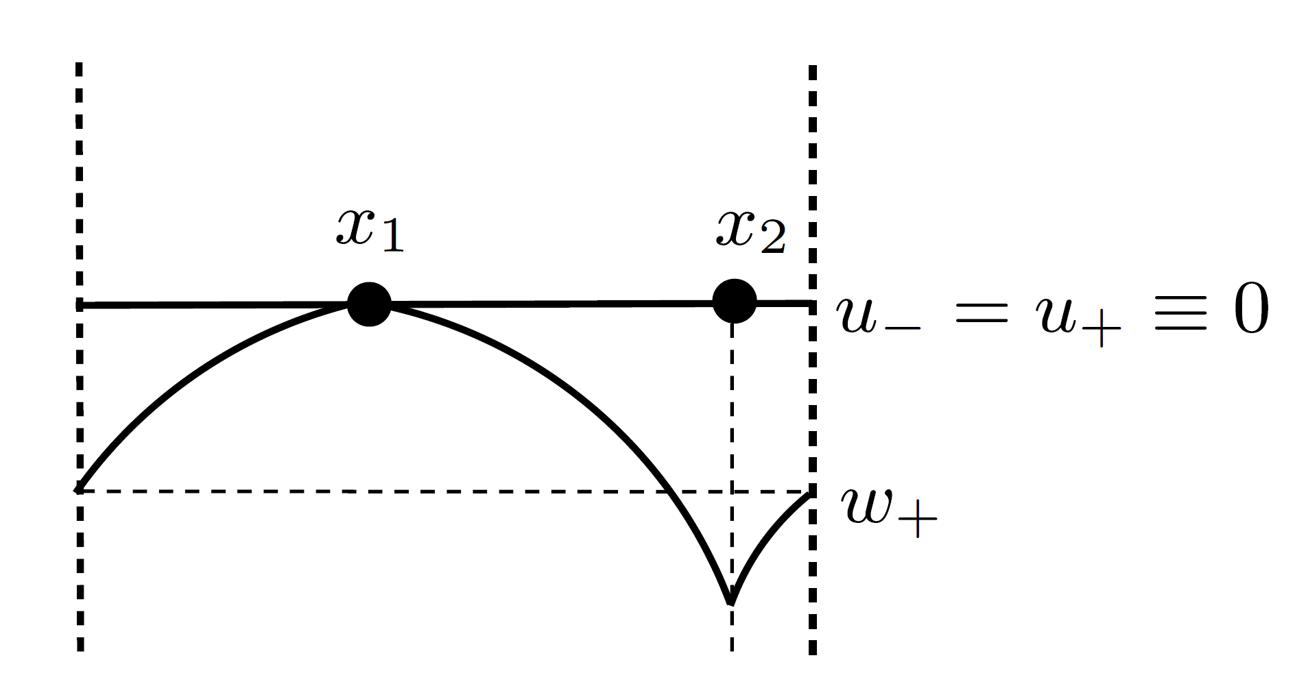
Figure 1. $\mathcal{S}_{\pm}$ in Item (iii)

2.2. Main results

First of all, we locate the strongly static set in a series of action minimizing invariant sets, and show its relations to the recurrence property and the non-wandering property.

Theorem 1 (Topological dynamics around the Aubry set).

Let $\tilde{\mathcal{R}}$ be the set of recurrent points. Let $\tilde{\Omega}$ be the set of non-wandering points. Then

$$\emptyset\neq\tilde{\mathcal{M}}\subseteq\tilde{\mathcal{N}}\cap\mathrm{cl}(\tilde{\mathcal{R}})\subseteq\tilde{\mathcal{S}}_{s}\subseteq\tilde{\mathcal{A}}\cap\tilde{\Omega}.$$

The closure $\text{cl}(\tilde{\mathcal{R}})$ is called the Birkhoff center. The fact $\tilde{\mathcal{M}}\subseteq\tilde{\mathcal{N}}\cap\mathrm{cl}(\tilde{\mathcal{R}})$ follows easily from the Poincaré recurrence theorem. To prove $\tilde{\mathcal{N}}\cap\mathrm{cl}(\tilde{\mathcal{R}})\subseteq\tilde{\mathcal{S}}_{s}$, we need to establish the Lipschitz continuity of the Mañé potentials, whose proof is postponed to A.2. The inclusion $\tilde{\mathcal{S}}_{s}\subseteq\tilde{\mathcal{A}}\cap\tilde{\Omega}$ follows from a technical lemma on transitive criterion (see Lemma 4.1 below).

In order to show the differences of the dynamics between the classical cases and the contact cases, we enhance the assumption (H3) by

• Strictly increasing: there is a constant $\lambda>0$ such that for every $(x,p,u)\in T^{\ast}M\times\mathbb{R}$,

  $$0<\frac{\partial H}{\partial u}(x,p,u)\leq\lambda,$$

Under (H1), (H2), (H3’) and (A), it is well known that the set of backward weak KAM solutions $\mathcal{S}_{-}$ consists of only one element. Consequently, the Mañé set coincides with the Aubry set (see [24, Remark 2]). However, the structure of the set of forward weak KAM solutions $\mathcal{S}_{+}$ may be rather complicated. That causes significant differences between the Aubry set and the strongly static set, as it is shown in Proposition 2.12.

In order to deal with the other elements in $\mathcal{S}_{+}$ except the maximal one. We define a partial ordering in $\mathcal{S}_{+}$:

$v_{1}\preceq v_{2}$ if and only if $v_{1}(x)\leq v_{2}(x)$ for all $x\in M$.

Moreover, we define $\mathcal{Z}_{\max}$ a maximal totally ordered subset of $\mathcal{S}_{+}$. Namely, for any $w_{+}\in\mathcal{S}_{+}\backslash\mathcal{Z}_{\max}$, there exist $v_{+}\in\mathcal{Z}_{\max}$ and $x_{1},x_{2}\in M$ such that $w_{+}(x_{2})>v_{+}(x_{2})$ and $w_{+}(x_{2})<v_{+}(x_{2})$. We will show the existence of minimal elements in $\mathcal{S}_{+}$ in this sense of partial ordering. Moreover, we will provide a representation for the minimal element in $\mathcal{Z}_{\max}$.

Theorem 2 (Minimal forward weak KAM solutions).

• The partially ordered set $(\mathcal{S}_{+},\preceq)$ has minimal elements.

• For each $\mathcal{Z}_{\max}\subseteq\mathcal{S}_{+}$, there exists $x_{0}\in\mathcal{M}$ depending on $\mathcal{Z}_{\max}$, such that the minimal element $u^{*}$ in $\mathcal{Z}_{\max}$ can be represented in the following two manners:

  $$u^{*}(x)=\inf_{\begin{subarray}{c}v_{+}(x_{0})=u_{-}(x_{0})\\ v_{+}\in\mathcal{S}_{+}\end{subarray}}v_{+}(x)=\limsup_{t\to+\infty}h^{x_{0},u_{-}(x_{0})}(x,t),$$

  where $\mathcal{M}$ denotes the projected Mather set and $h^{\cdot,\cdot}(\cdot,\cdot):M\times\mathbb{R}\times M\times\mathbb{R}_{+}\to\mathbb{R}$ is the action function defined by (2.4).

See Remark 6.8 below for a discussion on the choice of $x_{0}$, from which one can see that the strongly static set plays an essential role. By analysing more in details the structure of $\mathcal{S}_{+}$, one has

Theorem 3 (Existence of transitive orbits).

Given $X_{1}:=(x_{1},p_{1},u_{1})\in\tilde{\mathcal{A}}$, $X_{2}:=(x_{2},p_{2},u_{2})\in\tilde{\mathcal{S}}_{s}$, if for each $v_{+}\in\mathcal{S}_{+}$, $v_{+}(x_{2})=u_{-}(x_{2})$ implies $v_{+}(x_{1})=u_{-}(x_{1})$, then $X_{1}\rightsquigarrow X_{2}$.

If the forward weak KAM solution is unique, $\tilde{\mathcal{A}}=\tilde{\mathcal{S}}_{s}$ (see [24, Proposition 10]). In this case, the projected strongly static set can be characterized as follows

$$\mathcal{S}_{s}=\{x\in M\ |\ u_{-}(x)=u_{+}(x)\},$$

where $u_{-}$ (resp. $u_{+}$) denotes the unique backward (resp. forward) weak KAM solution. From Theorem 3, we have the following corollary.

Corollary 2.13.

Given any two points $X_{1},X_{2}\in\tilde{\mathcal{A}}$, if the forward weak KAM solution is unique, then $X_{1}\rightsquigarrow X_{2}$.

Figure 2 provides a rough picture for the dynamics around $\tilde{\mathcal{A}}$ (projected to $M\times\mathbb{R}$) under the assumption of Theorem 3, where

• $\Gamma_{t}$ denotes a transitive orbit from $X_{1}$ to $X_{2}$;

• $\Gamma_{n}^{1}$, $\Gamma_{n}^{2}$ denote non-wandering orbits to $X_{1}$ and $X_{2}$ respectively.

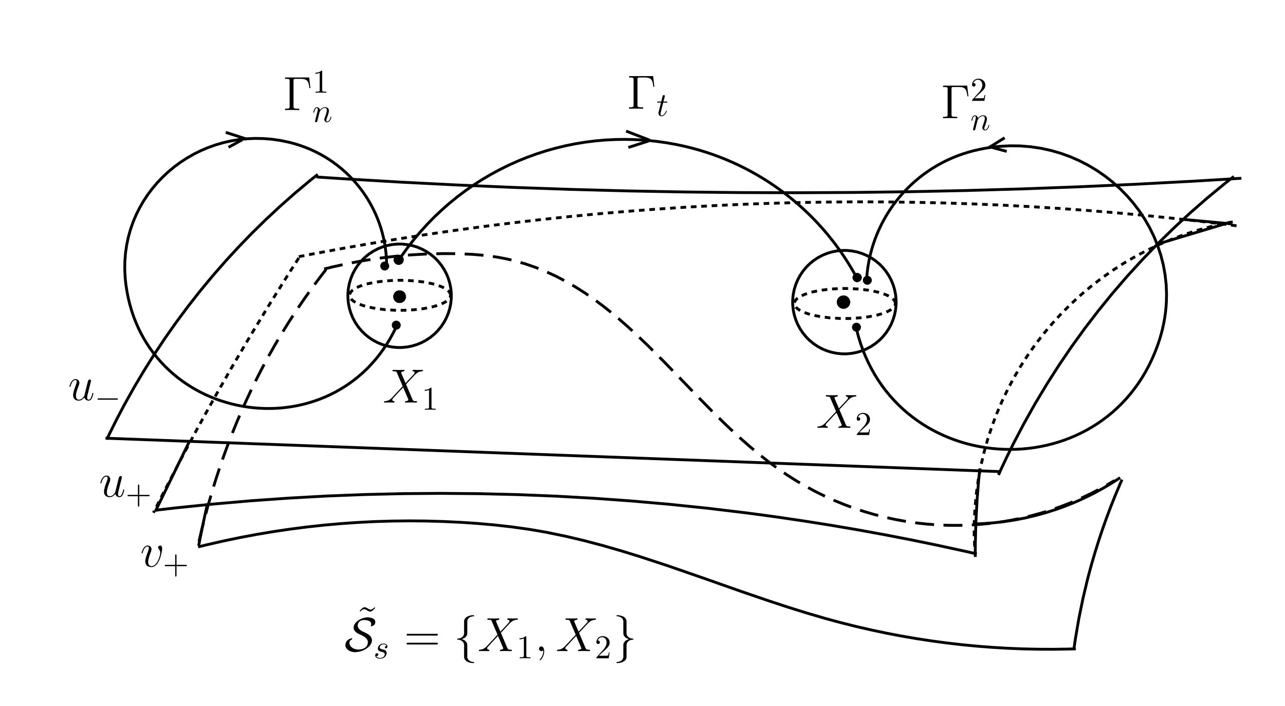
Figure 2. The dynamics around the Aubry set

The rest of this paper is organized as follows. In Section 3, we recall some useful facts, which mainly come from [22, 24]. In Section 4, we prove a technical lemma on the existence of certain transitive orbit, from which we obtain the topological dynamics around the Aubry set in Section 5. In Section 6, we provide more detailed information on the set of forward weak KAM solutions in the strictly increasing cases. Some auxiliary results are proved in A. Finally, we provide a proof of Proposition 2.12 in B.

3. Preliminaries

Different from classical cases, all of technical tools for contact Hamiltonian systems were formed in an implicit manner. The main reason to use the implicit form is to get rid of the constraints caused by the $u$-argument. Besides, it is worth mentioning that an alternative variational formulation was provided in [2, 12] in light of G. Herglotz’s work [10].

In the following, we collect some facts used in this paper. All of these results hold under (H1), (H2) and $|\partial_{u}H|\leq\lambda$.

3.1. Action functions and minimizing curves

Let us collect some properties of the action functions $h_{x_{0},u_{0}}(x,t)$ and $h^{x_{0},u_{0}}(x,t)$ in the following propositions. See [20, Theorems C, D] and [21, Theorem 3.1, Propositions 3.1-3.4] for more details.

Proposition 3.1.

• (Monotonicity). Given $x_{0}\in M$, $u_{0}$, $u_{1}$, $u_{2}\in\mathbb{R}$, if $u_{1}<u_{2}$, then $h_{x_{0},u_{1}}(x,t)<h_{x_{0},u_{2}}(x,t)$, for all $(x,t)\in M\times(0,+\infty)$;

• (Minimality). Given $x_{0}$, $x\in M$, $u_{0}\in\mathbb{R}$ and $t>0$, let $S^{x,t}_{x_{0},u_{0}}$ be the set of the solutions $(x(s),p(s),u(s))$ of (1.4) on $[0,t]$ with $x(0)=x_{0}$, $x(t)=x$, $u(0)=u_{0}$. Then

  $$h_{x_{0},u_{0}}(x,t)=\inf\{u(t)\ |\ (x(s),p(s),u(s))\in S^{x,t}_{x_{0},u_{0}}\},\quad\forall(x,t)\in M\times(0,+\infty).$$

• (Lipschitz continuity). The function $(x_{0},u_{0},x,t)\mapsto h_{x_{0},u_{0}}(x,t)$ is locally Lipschitz continuous on $M\times\mathbb{R}\times M\times(0,+\infty)$.

• (Markov property). Given $x_{0}\in M$, $u_{0}\in\mathbb{R}$,

  $$h_{x_{0},u_{0}}(x,t+s)=\inf_{y\in M}h_{y,h_{x_{0},u_{0}}(y,t)}(x,s)$$

  for all $s$, $t>0$ and all $x\in M$. Moreover, the infimum is attained at $y$ if and only if there exists a minimizer $\gamma$ of $h_{x_{0},u_{0}}(x,t+s)$ with $\gamma(t)=y$.

• (Reversibility). Given $x_{0}$, $x\in M$ and $t>0$, for each $u\in\mathbb{R}$, there exists a unique $u_{0}\in\mathbb{R}$ such that

  $$h_{x_{0},u_{0}}(x,t)=u.$$

Proposition 3.2.

• (Monotonicity). Given $x_{0}\in M$ and $u_{1}$, $u_{2}\in\mathbb{R}$, if $u_{1}<u_{2}$, then $h^{x_{0},u_{1}}(x,t)<h^{x_{0},u_{2}}(x,t)$, for all $(x,t)\in M\times(0,+\infty)$;

• (Maximality). Given $x_{0}$, $x\in M$, $u_{0}\in\mathbb{R}$ and $t>0$, let $S_{x,t}^{x_{0},u_{0}}$ be the set of the solutions $(x(s),p(s),u(s))$ of (1.4) on $[0,t]$ with $x(0)=x$, $x(t)=x_{0}$, $u(t)=u_{0}$. Then

  $$h^{x_{0},u_{0}}(x,t)=\sup\{u(0)\ |\ (x(s),p(s),u(s))\in S_{x,t}^{x_{0},u_{0}}\},\quad\forall(x,t)\in M\times(0,+\infty).$$

• (Lipschitz continuity). The function $(x_{0},u_{0},x,t)\mapsto h^{x_{0},u_{0}}(x,t)$ is locally Lipschitz continuous on $M\times\mathbb{R}\times M\times(0,+\infty)$.

• (Markov property). Given $x_{0}\in M$, $u_{0}\in\mathbb{R}$,

  $$h^{x_{0},u_{0}}(x,t+s)=\sup_{y\in M}h^{y,h^{x_{0},u_{0}}(y,t)}(x,s)$$

  for all $s$, $t>0$ and all $x\in M$. Moreover, the supremum is attained at $y$ if and only if there exists a minimizer $\gamma$ of $h^{x_{0},u_{0}}(x,t+s)$, such that $\gamma(t)=y$.

• (Reversibility). Given $x_{0}$, $x\in M$, and $t>0$, for each $u\in\mathbb{R}$, there exists a unique $u_{0}\in\mathbb{R}$ such that

  $$h^{x_{0},u_{0}}(x,t)=u.$$

By definition, we have

Proposition 3.3.

Let $(x(\cdot),u(\cdot)):\mathbb{R}\to M\times\mathbb{R}$ be a globally minimizing curve. Then for all $t_{1}$, $t_{2}\in\mathbb{R}$ with $t_{1}\leq t_{2}$,

$$u(t_{2})=\inf_{s>0}h_{x(t_{1}),u(t_{1})}(x(t_{2}),s)\text{\ \ if\ and\ only\ if\ \ }u(t_{1})=\sup_{s>0}h^{x(t_{2}),u(t_{2})}(x(t_{1}),s).$$

Remark 3.4.

By Proposition 3.3,

• a curve $(x(\cdot),u(\cdot)):\mathbb{R}\to M\times\mathbb{R}$ is globally minimizing if and only if for each $t_{1}<t_{2}\in\mathbb{R}$,

  $$u(t_{1})=h^{x(t_{2}),u(t_{2})}(x(t_{1}),t_{2}-t_{1});$$ (3.1)

• a curve $(x(\cdot),u(\cdot)):\mathbb{R}\to M\times\mathbb{R}$ is semi-static if and only if it is globally minimizing and for each $t_{1}\leq t_{2}\in\mathbb{R}$,

  $$u(t_{1})=\sup_{s>0}h^{x(t_{2}),u(t_{2})}(x(t_{1}),s);$$ (3.2)

• a positively (resp. negatively) semi-static curve can be also characterized in a similar manner.

3.2. Lax-Oleinik semigroups, weak KAM solutions and the Mañé set

Let us recall two semigroups of operators introduced in [21]. Define a family of nonlinear operators $\{T^{-}_{t}\}_{t\geq 0}$ from $C(M,\mathbb{R})$ to itself as follows. For each $\varphi\in C(M,\mathbb{R})$, denote by $(x,t)\mapsto T^{-}_{t}\varphi(x)$ the unique continuous function on $M\times[0,+\infty)$ such that

$$T^{-}_{t}\varphi(x)=\inf_{\gamma}\left\{\varphi(\gamma(0))+\int_{0}^{t}L(\gamma(\tau),\dot{\gamma}(\tau),T^{-}_{\tau}\varphi(\gamma(\tau)))d\tau\right\},$$

where the infimum is taken among absolutely continuous curves $\gamma:[0,t]\to M$ with $\gamma(t)=x$. Let $\gamma$ be a curve achieving the infimum, and $x(s):=\gamma(s)$, $u(s):=T_{s}^{-}\varphi(x(s))$, $p(s):=\frac{\partial L}{\partial\dot{x}}(x(s),\dot{x}(s),u(s))$. Then $(x(s),p(s),u(s))$ satisfies (1.4) with $x(t)=x$.

It is not difficult to see that $\{T^{-}_{t}\}_{t\geq 0}$ is a semigroup of operators and $T^{-}_{t}\varphi(x)$ is a viscosity solution of $w_{t}+H(x,w,w_{x})=0$ with $w(x,0)=\varphi(x)$.

Similarly, one can define another semigroup of operators $\{T^{+}_{t}\}_{t\geq 0}$ by

$$T^{+}_{t}\varphi(x)=\sup_{\gamma}\left\{\varphi(\gamma(t))-\int_{0}^{t}L(\gamma(\tau),\dot{\gamma}(\tau),T^{+}_{t-\tau}\varphi(\gamma(\tau)))d\tau\right\},$$

where the infimum is taken among absolutely continuous curves $\gamma:[0,t]\to M$ with $\gamma(0)=x$. Let $\gamma$ be a curve achieving the infimum, and $x(s):=\gamma(s)$, $u(s):=T_{t-s}^{+}\varphi(x(s))$, $p(s):=\frac{\partial L}{\partial\dot{x}}(x(s),\dot{x}(s),u(s))$. Then $(x(s),p(s),u(s))$ satisfies (1.4) with $x(0)=x$.

The following proposition gives a relation between Lax-Oleinik semigroups and action functions. See [21, Propositions 4.1, 4.2] for details.

Proposition 3.5.

For each $\varphi\in C(M,\mathbb{R})$, we have

$$T^{-}_{t}\varphi(x)=\inf_{y\in M}h_{y,\varphi(y)}(x,t),\quad T^{+}_{t}\varphi(x)=\sup_{y\in M}h^{y,\varphi(y)}(x,t),\quad\forall(x,t)\in M\times(0,+\infty).$$

The following proposition gives a relation between Lax-Oleinik semigroups and weak KAM solutions. See [19, Lemmas 4.1, 4.2, 6.2] for details.

Proposition 3.6.

The backward weak KAM solutions of (HJ) are the same as the viscosity solutions of (HJ). Moreover,

• A function $u:M\to\mathbb{R}$ is a backward weak KAM solution of (HJ) if and only if $T^{-}_{t}u=u$ for all $t\geq 0$;

• A function $v:M\to\mathbb{R}$ is a forward weak KAM solution of (HJ) if and only if $T^{+}_{t}v=v$ for all $t\geq 0$.

By [22, Theorem 1.2] and [23, Theorem 1], we have

Proposition 3.7.

$\mathcal{S}_{-}\neq\emptyset$ if and only if $\mathcal{S}_{+}\neq\emptyset$. More precisely, the following statements hold.

• Let $v_{-}\in\mathcal{S}_{-}$. Then the function $x\mapsto\lim_{t\rightarrow\infty}T_{t}^{+}v_{-}(x)$ is well defined, and it belongs to $\mathcal{S}_{+}$.

• Let $v_{+}\in\mathcal{S}_{+}$. Then the function $x\mapsto\lim_{t\rightarrow\infty}T_{t}^{-}v_{+}(x)$ is well defined, and it belongs to $\mathcal{S}_{-}$.

In the following context of this section, we proceed under the assumption $\mathcal{S}_{-}\neq\emptyset$. Here we recall that the assumption $\mathcal{S}_{-}\neq\emptyset$ is equivalent to assumption (A). It is well known that each $u_{-}\in\mathcal{S}_{-}$ is semiconcave and $u_{+}\in\mathcal{S}_{+}$ is semiconvex. For each $u_{\pm}\in\mathcal{S}_{\pm}$, we define two subsets of $T^{*}M\times\mathbb{R}$ associated with $u_{\pm}$ respectively by

$$G_{u_{\pm}}:=\mathrm{cl}\left(\big{\{}(x,p,u)\ |\ Du_{\pm}(x)\ \text{exists},\ u=u_{\pm}(x),\ p=Du_{\pm}(x)\big{\}}\right),$$ (3.3)

where $\mathrm{cl}(A)$ denotes the closure of $A\subseteq T^{*}M\times\mathbb{R}$. Define

$$\tilde{\mathcal{N}}_{v_{\pm}}:=\tilde{\mathcal{N}}\cap G_{v_{\pm}},\quad\mathcal{N}_{v_{\pm}}:=\pi^{*}\tilde{\mathcal{N}}_{v_{\pm}}.$$

The following proposition shows a relation between weak KAM solutions and semi-static curves. See [24, Proposition 17] for details.

Proposition 3.8.

Let $(x(\cdot),u(\cdot)):\mathbb{R}\rightarrow M\times\mathbb{R}$ be a semi-static curve. Then there exists $v_{-}\in\mathcal{S}_{-}$ (resp. $v_{+}\in\mathcal{S}_{+}$) such that $u(t)=v_{-}(x(t))$ (resp. $u(t)=v_{+}(x(t)$) for each $t\in\mathbb{R}$.

The following proposition shows a relation between weak KAM solutions and the Mañé set. See [24, Theorem 1.3] for details.

Proposition 3.9.

Let $v_{-}\in\mathcal{S}_{-}$, $v_{+}\in\mathcal{S}_{+}$. Let

$$\mathcal{I}_{v_{-}}:=\{x\in M\ |\ v_{-}(x)=\lim_{t\rightarrow\infty}T_{t}^{+}v_{-}(x)\}$$

$$\mathcal{I}_{v_{+}}:=\{x\in M\ |\ v_{+}(x)=\lim_{t\rightarrow\infty}T_{t}^{-}v_{+}(x)\}.$$

Then both $\mathcal{I}_{v_{-}}$ and $\mathcal{I}_{v_{+}}$ are not empty. Moreover,

$$\tilde{\mathcal{N}}_{v_{\pm}}=\{(x,p,u)\in T^{*}M\times\mathbb{R}\ |\ x\in\mathcal{I}_{v_{\pm}},\ u=v_{\pm}(x),\ p=Dv_{\pm}(x)\},$$

$$\tilde{\mathcal{N}}=\cup_{v_{-}\in\mathcal{S}_{-}}\tilde{\mathcal{N}}_{v_{-}}=\cup_{v_{+}\in\mathcal{S}_{+}}\tilde{\mathcal{N}}_{v_{+}}.$$

4. A technical lemma

In this section, we are devoted to proving a technical lemma on the existence of certain transitive orbit. It will be used in the proofs of Theorem 1 and Theorem 3.

Lemma 4.1 (Transitive criterion).

Given $X_{1}:=(x_{1},p_{1},u_{1})\in\tilde{\mathcal{A}}$, $X_{2}:=(x_{2},p_{2},u_{2})\in\tilde{\mathcal{S}}_{s}$. If

$$\lim_{t\to+\infty}h_{x_{1},u_{1}}(x_{2},t)=u_{2},\ \limsup_{t\to+\infty}h^{x_{2},u_{2}}(x_{1},t)=u_{1}, \diamondsuit$$ ()

then $X_{1}\rightsquigarrow X_{2}$.

Remark 4.2.

This criterion can be viewed as a technical trick. Loosely speaking, it means that under the condition ($\diamondsuit$), certain orbit $(x(\cdot),p(\cdot),u(\cdot)):\mathbb{R}\to T^{*}M\times\mathbb{R}$ can be controlled by its $x$ and $u$-arguments. Under (H1)-(H3) and (A), we consider the following two functions

$$A(x):=\lim_{t\to+\infty}h_{x_{1},u_{1}}(x,t),\quad B(x):=\limsup_{t\to+\infty}h^{x_{2},u_{2}}(x,t).$$

Due to (H3), the limit function $A:M\to\mathbb{R}$ is well defined. In general, $h^{x_{2},u_{2}}(x,t)$ diverges as $t\to+\infty$. But we have the existence of $B(x)$ if there exists a semi-static curve $(x(\cdot),u(\cdot)):\mathbb{R}\to M\times\mathbb{R}$ passing through $(x_{2},u_{2})$ (see Lemma A.4). Then $A(x)$ and $B(x)$ can be viewed as two Peierls barriers for contact Hamiltonian systems.

If $H$ is independent of $u$, the condition ($\diamondsuit$) is reduced to

$$h^{\infty}(x_{1},x_{2})=u_{2}-u_{1},$$

where $h^{\infty}:M\times M\to\mathbb{R}$ is the Peierls barrier in the classical case. Given any two points in the Aubry set in $T^{*}M$, this condition always holds if we choose a suitable embedding manner from $T^{*}M$ to $T^{*}M\times\mathbb{R}$.

In general cases, it is not easy to be verified. Under (H1)-(H3) and (A), we are able to use this criterion to prove the non-wandering property of the strongly static set, for which it suffices to consider the case with $X_{1}=X_{2}$. For the case with $X_{1}\neq X_{2}$, we consider this criterion in strictly increasing cases (H3’). In Theorem 3, it shows that the criterion can be verified by assuming “if for each $v_{+}\in\mathcal{S}_{+}$, $v_{+}(x_{2})=u_{-}(x_{2})$ implies $v_{+}(x_{1})=u_{-}(x_{1})$”. That shows the interplay between weak KAM solutions and the dynamics around the Aubry set.

Let $\tilde{\mathcal{V}}$ be the set of $(x,p,u)\in T^{*}M\times\mathbb{R}$, for which there exists a strongly static orbit

$$(x(\cdot),p(\cdot),u(\cdot)):\mathbb{R}\to T^{*}M\times\mathbb{R}$$

passing through $(x,p,u)$. Let ${\mathcal{V}}=\pi^{*}\tilde{\mathcal{V}}$. By the definition of the strongly static set,

$$\tilde{\mathcal{S}}_{s}=\mathrm{cl}(\tilde{\mathcal{V}}),\quad\mathcal{S}_{s}=\mathrm{cl}(\mathcal{V}).$$

To prove Lemma 4.1, we only need to verify

Lemma 4.3.

Given any $X_{1}:=(x_{1},p_{1},u_{1})\in\tilde{\mathcal{A}}$, $X_{2}:=(x_{2},p_{2},u_{2})\in\tilde{\mathcal{V}}$. If

$$\lim_{t\to+\infty}h_{x_{1},u_{1}}(x_{2},t)=u_{2},\ \limsup_{t\to+\infty}h^{x_{2},u_{2}}(x_{1},t)=u_{1},$$

then $X_{1}\rightsquigarrow X_{2}$.

We give a proof that Lemma 4.3 implies Lemma 4.1.

Proof.

Let $B(X,R)$ stand for the open ball on $T^{*}M\times\mathbb{R}$ centered at $X$ with radius $R$, and let $\bar{B}(X,R)$ stand for its closure.

Given any $X_{2}:=(x_{2},p_{2},u_{2})\in\tilde{\mathcal{S}}_{s}$. For any neighborhood $U$ of $X_{2}$, one can find $R>0$ such that $\bar{B}(X_{2},R)\subset U$. Note that $\tilde{\mathcal{S}}_{s}=\mathrm{cl}(\tilde{\mathcal{V}})$. Thus, there exists a sequence $\{Z_{n}\}_{n\in\mathbb{N}}\subseteq\tilde{\mathcal{V}}$ such that

$$Z_{n}\to X_{2},\quad n\to\infty.$$

Hence, there exists $N:=N(R)>0$ such that

$$d(X_{2},Z_{N})\leq\frac{R}{4},$$

which implies

$$B\left(Z_{N},\frac{R}{4}\right)\subset B(X_{2},R).$$

By Definition 1.1, the existence of the transitive orbit from $X_{1}$ to $Z_{N}$ implies $X_{1}\rightsquigarrow X_{2}$. ∎

The following lemma gives a way to obtain one-sided semi-static curves from one-sided minimizing curves.

Lemma 4.4.

• Given $(x_{0},u_{0})\in M\times\mathbb{R}$, let $({x}(\cdot),{u}(\cdot)):\mathbb{R}_{+}\to M\times\mathbb{R}$ be a positively minimizing curve with $(x(0),u(0))=(x_{0},u_{0})$. If for each $t\geq 0$,

  $${u}(t)=\inf_{\tau>0}h_{x_{0},u_{0}}({x}(t),\tau).$$ (4.1)

  Then for any $t_{1}$, $t_{2}\in\mathbb{R}_{+}$ with $t_{1}\leq t_{2}$, there holds

  $${u}(t_{2})=\inf_{\tau>0}h_{{x}(t_{1}),{u}(t_{1})}({x}(t_{2}),\tau).$$ (4.2)

• Given $(x_{0},u_{0})\in M\times\mathbb{R}$, let $({x}(\cdot),{u}(\cdot)):\mathbb{R}_{-}\to M\times\mathbb{R}$ be a negatively minimizing curve with $(x(0),u(0))=(x_{0},u_{0})$. If for each $t\geq 0$,

  $${u}(-t)=\sup_{\tau>0}h^{x_{0},u_{0}}({x}(-t),\tau).$$ (4.3)

  Then for any $t_{1}$, $t_{2}\in\mathbb{R}_{+}$ with $t_{1}\geq t_{2}$, there holds

  $${u}(-t_{1})=\sup_{\tau>0}h^{{x}(-t_{2}),{u}(-t_{2})}({x}(-t_{1}),\tau).$$ (4.4)

Proof.

We only prove Item (1). Item (2) follows from a similar argument. Since $({x}(\cdot),{u}(\cdot)):\mathbb{R}_{+}\to M\times\mathbb{R}$ is positively minimizing, then

$${u}(t_{2})\geq\inf_{\tau>0}h_{{x}(t_{1}),{u}(t_{1})}({x}(t_{2}),\tau),\quad\forall\ 0\leq t_{1}<t_{2}.$$ (4.5)

By assumption, for each $t\geq 0$,

$${u}(t)=\inf_{\tau>0}h_{x_{0},u_{0}}({x}(t),\tau).$$ (4.6)

It follows that

$${u}(t_{1})=\inf_{\tau>0}h_{x_{0},u_{0}}({x}(t_{1}),\tau),\quad{u}(t_{2})=\inf_{\tau>0}h_{x_{0},u_{0}}({x}(t_{2}),\tau),$$

which gives rise to

$${u}(t_{2}) =\inf_{\tau>0}h_{x_{0},u_{0}}({x}(t_{2}),\tau)\leq\inf_{\tau>0}h_{x_{0},u_{0}}({x}(t_{2}),t_{1}+\tau)$$

$$\leq\inf_{\tau>0}h_{{x}(t_{1}),h_{x_{0},u_{0}}({x}(t_{1}),t_{1})}({x}(t_{2}),\tau)$$

$$=\inf_{\tau>0}h_{{x}(t_{1}),{u}(t_{1})}({x}(t_{2}),\tau).$$

Combining with (4.5), we get (4.2). ∎

The following proposition shows that for certain minimizing orbits $(x(\cdot),p(\cdot),u(\cdot)):\mathbb{R}\rightarrow T^{*}M\times\mathbb{R}$, $p(t)$ is uniquely determined by $(x(t),u(t))$ for all $t\in\mathbb{R}$. Let $\rho:\tilde{\mathcal{V}}\to M\times\mathbb{R}$. This result implies $\rho$ is injective, which gives rise to the graph property of $\tilde{\mathcal{V}}$ on $M\times\mathbb{R}$. Its proof is postponed in A.1.

Proposition 4.5.

If $(x,p_{0},u)\in{\tilde{\mathcal{V}}}$, $(x,p_{+},u)\in\tilde{\mathcal{N}}^{+}$ (resp. $(x,p_{-},u)\in\tilde{\mathcal{N}}^{-}$), then $p_{0}=p_{+}$ (resp. $p_{0}=p_{-}$).

Under the assumptions (H1)-(H3), by the definitions of $h_{x_{0},u_{0}}(x,t)$ and $h^{x_{0},u_{0}}(x,t)$, we have

Proposition 4.6.

Given $(x_{0},x,t)\in M\times M\times(0,+\infty)$, $u,v\in\mathbb{R}$.

• for all $u$, $v\in\mathbb{R}$ and all $(x,t)\in M\times(0,+\infty)$, $|h_{x_{0},u}(x,t)-h_{x_{0},v}(x,t)|\leq|u-v|$;

• if $u\geq v$, then $h^{x_{0},u}(x,t)-h^{x_{0},v}(x,t)\geq u-v$.

Proof of Lemma 4.3. Let $\{t_{n}\}_{n\in\mathbb{N}}$ be a sequence satisfying

$$\lim_{t_{n}\to+\infty}h^{x_{2},u_{2}}(x_{1},t_{n})=u_{1}.$$

Let $\gamma_{n}:[0,t_{n}]\rightarrow M$ be a curve $\gamma_{n}(0)=x_{1}$ and $\gamma_{n}(t_{n})=x_{2}$ such that

$$h^{x_{2},u_{2}}(x_{1},t_{n})=u_{2}-\int_{0}^{t_{n}}L\big{(}\gamma_{n}(\tau),\dot{\gamma}_{n}(\tau),h^{x_{2},u_{2}}(\gamma_{n}(\tau),t_{n}-\tau)\big{)}d\tau.$$ (4.7)

Let $u_{n}(t):=h^{x_{2},u_{2}}(\gamma_{n}(t),t_{n}-t)$. Then $u_{n}(t_{n})=u_{2}$ and $u_{n}(0)=h^{x_{2},u_{2}}(x_{1},t_{n})$. Let

$$p_{n}(t):=\frac{\partial L}{\partial\dot{x}}(\gamma_{n}(t),\dot{\gamma}_{n}(t),u_{n}(t)).$$

We claim that there exists $C>0$ such that

$$\|p_{n}(0)\|_{x_{1}}\leq C,\quad\|p_{n}(t_{n})\|_{x_{2}}\leq C.$$

In fact, since $u_{n}(0)\rightarrow u_{1}$ as $n\rightarrow+\infty$, combining with the compactness of $M$, then

$$u_{n}(1)=h^{x_{2},u_{2}}(\gamma_{n}(1),t_{n}-1)=h_{x_{1},u_{n}(0)}(\gamma_{n}(1),1)$$

is bounded independently on $n$. Similarly, $u_{n}(t_{n}-1)=h^{x_{2},u_{2}}(\gamma_{n}(t_{n}-1),1)$ are bounded independent of $n$. Note that $u_{n}(t_{n})=u_{2}$. Then one can find $C>0$ such that both $p_{n}(0)$ and $p_{n}(t_{n})$ is bounded by $C$ (see [21, Appendix, proof of Lemma 2.1] for details).

We assume, up to a subsequence,

$$(\gamma_{n}(0),p_{n}(0),u_{n}(0))\rightarrow(x_{1},p^{\prime}_{1},u_{1}),\quad(\gamma_{n}(t_{n}),p_{n}(t_{n}),u_{n}(t_{n}))\rightarrow(x_{2},p^{\prime}_{2},u_{2}).$$

In order to prove Lemma 4.3, it suffices to verify

$$p^{\prime}_{1}=p_{1},\quad p^{\prime}_{2}=p_{2}.$$

First of all, we prove $p^{\prime}_{1}=p_{1}$. By Proposition 4.5, we only need to show $(x_{1},p^{\prime}_{1},u_{1})\in\tilde{\mathcal{N}}^{+}$. Let

$$(\bar{x}(t),\bar{p}(t),\bar{u}(t)):=\Phi_{t}(x_{1},p^{\prime}_{1},u_{1}),\quad\forall t\geq 0.$$

By the definition of $\tilde{\mathcal{N}}^{+}$, we need to show that

• the curve $(\bar{x}(\cdot),\bar{u}(\cdot)):\mathbb{R}_{+}\to M\times\mathbb{R}$ is positively minimizing;

• for any $t_{1}$, $t_{2}\in\mathbb{R}_{+}$ with $t_{1}\leq t_{2}$, there holds

  $$\bar{u}(t_{2})=\inf_{\tau>0}h_{\bar{x}(t_{1}),\bar{u}(t_{1})}(\bar{x}(t_{2}),\tau).$$ (4.8)

Since $\gamma_{n}:[0,t_{n}]\rightarrow M$ satisfies (4.7), by the definition of $u_{n}(t)$, we have

$$u_{n}(t_{1})=h^{\gamma_{n}(t_{2}),u_{n}(t_{2})}(\gamma_{n}(t_{1}),t_{2}-t_{1}),\quad\forall 0\leq t_{1}<t_{2}\leq t_{n}.$$

By the continuous dependence of solutions to ODEs on the initial data,

$$(\gamma_{n}(t_{1}),u_{n}(t_{1}))\to(\bar{x}(t_{1}),\bar{u}(t_{1})),\quad(\gamma_{n}(t_{2}),u_{n}(t_{2}))\to(\bar{x}(t_{2}),\bar{u}(t_{2})),$$

which combining with the Lipschitz continuity of $(x_{0},u_{0},x)\mapsto h^{\cdot,\cdot}(\cdot,t_{2}-t_{1})$ yields

$$\bar{u}(t_{1})=h^{\bar{x}(t_{2}),\bar{u}(t_{2})}(\bar{x}(t_{1}),t_{2}-t_{1}),\quad\forall 0\leq t_{1}<t_{2}<+\infty.$$

By Remark 3.4, $(\bar{x}(\cdot),\bar{u}(\cdot)):\mathbb{R}_{+}\to M\times\mathbb{R}$ is positively minimizing. In order to verify Item (2), by Lemma 4.4(1), we need to prove that for each $t\geq 0$,

$$\bar{u}(t)=\inf_{\tau>0}h_{x_{1},u_{1}}(\bar{x}(t),\tau).$$ (4.9)

By definition, we have

$$\bar{u}(t)\geq\inf_{\tau>0}h_{x_{1},u_{1}}(\bar{x}(t),\tau).$$

It suffices to show

$$\bar{u}(t)\leq\inf_{\tau>0}h_{x_{1},u_{1}}(\bar{x}(t),\tau).$$

By contradiction, we assume there exist $t_{0},\tau_{0}>0$ such that

$$\bar{u}(t_{0})>h_{x_{1},u_{1}}(\bar{x}(t_{0}),\tau_{0}).$$

By Proposition 4.6(2), one can find $\delta>0$ such that

$$h^{\bar{x}(t_{0}),\bar{u}(t_{0})}(x_{1},\tau_{0})=u_{1}+\delta.$$ (4.10)

For each $\varepsilon>0$, there exists $n$ large enough such that

$$d((\gamma_{n}(t_{0}),p_{n}(t_{0}),u_{n}(t_{0})),(\bar{x}(t_{0}),\bar{p}(t_{0}),\bar{u}(t_{0})))<\varepsilon,$$

which combining with Lipschitz continuity of $(x_{0},u_{0})\mapsto h^{\cdot,\cdot}(x_{1},\tau_{0})$ implies

$$h^{\gamma_{n}(t_{0}),u_{n}(t_{0})}(x_{1},\tau_{0})\geq u_{1}+\frac{\delta}{2}.$$

Note that $\gamma_{n}(t_{n})=x_{2}$, $\gamma_{n}(0)=x_{1}$, $u_{n}(t_{n})=u_{2}$. It follows that

$$h^{x_{2},u_{2}}(x_{1},t_{n}-t_{0}+\tau_{0}) =h^{\gamma_{n}(t_{n}),u_{n}(t_{n})}(\gamma_{n}(0),t_{n}-t_{0}+\tau_{0})$$

$$\geq h^{\gamma_{n}(t_{0}),h^{\gamma_{n}(t_{n}),u_{n}(t_{n})}(\gamma_{n}(t_{0}),t_{n}-t_{0})}(\gamma_{n}(0),\tau_{0})$$

$$=h^{\gamma_{n}(t_{0}),u_{n}(t_{0})}(\gamma_{n}(0),\tau_{0})$$

$$\geq u_{1}+\frac{\delta}{2}.$$

By assumption, $\limsup_{t\to+\infty}h^{x_{2},u_{2}}(x_{1},t)=u_{1}$. Letting $n\rightarrow+\infty$, we have $u_{1}>u_{1}$, which is a contradiction.

Next, we prove $p^{\prime}_{2}=p_{2}$. By Proposition 4.5, we only need to show $(x_{2},p^{\prime}_{2},u_{2})\in\tilde{\mathcal{N}}^{-}$. Let

$$(\tilde{x}(-t),\tilde{p}(-t),\tilde{u}(-t)):=\Phi_{-t}(x_{2},p^{\prime}_{2},u_{2}),\quad\forall 0\leq t<+\infty.$$

We aim to show that

• the curve $(\tilde{x}(\cdot),\tilde{u}(\cdot)):\mathbb{R}_{-}\to M\times\mathbb{R}$ is negatively minimizing;

• for any $t_{1}$, $t_{2}\in\mathbb{R}_{+}$ with $t_{1}\geq t_{2}$, there holds

  $$\tilde{u}(-t_{1})=\sup_{\tau>0}h^{\tilde{x}(-t_{2}),\tilde{u}(-t_{2})}(\tilde{x}(-t_{1}),\tau).$$ (4.11)

The proof of Item (1) is similar to the one of $p^{\prime}_{1}=p_{1}$ above.

Let $\eta_{n}(-t):=\gamma_{n}(-t+t_{n})$ for each $t\geq 0$. It follows that $\eta_{n}:[-t_{n},0]\rightarrow M$ satisfies (4.7) with $\eta_{n}(0)=x_{2}$, $\eta_{n}(-t_{n})=x_{1}$. Let $v_{n}(-t):=h^{x_{2},u_{2}}(\eta_{n}(-t),t)$ for each $t\geq 0$. Then $v_{n}(0)=u_{2}$ and

$$v_{n}(-t_{1})=h^{\eta_{n}(-t_{2}),v_{n}(-t_{2})}(\eta_{n}(-t_{1}),t_{1}-t_{2}),\quad\forall 0\leq t_{2}<t_{1}<t_{n}.$$ (4.12)

By (4.12),

$$v_{n}(-t_{0})=h_{\eta_{n}(-t_{n}),v_{n}(-t_{n})}(\eta_{n}(-t_{0}),t_{n}-t_{0}).$$ (4.13)

Similar to the proof of (4.10), we have

$$h_{\eta_{n}(-t_{0}),v_{n}(-t_{0})}(x_{2},\tau_{0})\leq u_{2}-\frac{\delta}{2}.$$ (4.14)

By Proposition 4.6(1),

$$\begin{split}&|h_{\eta_{n}(-t_{0}),h_{x_{1},u_{1}}(\eta_{n}(-t_{0}),t_{n}-t_{0})}(x_{2},\tau_{0})-h_{\eta_{n}(-t_{0}),h_{x_{1},v_{n}(-t_{n})}(\eta_{n}(-t_{0}),t_{n}-t_{0})}(x_{2},\tau_{0})|\\ \leq&|h_{x_{1},u_{1}}(\eta_{n}(-t_{0}),t_{n}-t_{0})-h_{x_{1},v_{n}(-t_{n})}(\eta_{n}(-t_{0}),t_{n}-t_{0})|\\ \leq&|u_{1}-v_{n}(-t_{n}))|.\end{split}$$ (4.15)

Then we have

$$h_{x_{1},u_{1}}(x_{2},t_{n}-t_{0}+\tau_{0}) \leq h_{\eta_{n}(-t_{0}),h_{x_{1},u_{1}}(\eta_{n}(-t_{0}),t_{n}-t_{0})}(x_{2},\tau_{0})$$

$$\leq h_{\eta_{n}(-t_{0}),h_{x_{1},v_{n}(-t_{n})}(\eta_{n}(-t_{0}),t_{n}-t_{0})}(x_{2},\tau_{0})+|u_{1}-v_{n}(-t_{n})|$$

$$=h_{\eta_{n}(-t_{0}),v_{n}(-t_{0})}(x_{2},\tau_{0})+|u_{1}-v_{n}(-t_{n})|$$

$$\leq u_{2}-\frac{\delta}{2}+|u_{1}-v_{n}(-t_{n})|,$$

where the first inequality is from the Markov property of $h_{x_{1},u_{1}}(x,t)$, the second inequality is owing to (4.15), the first equality is from (4.13), and the last inequality is from (4.14).

Note that $\eta_{n}(-t_{n})=x_{1}$, $\eta_{n}(0)=x_{2}$, $v_{n}(0)=u_{2}$. By assumption, $h^{x_{2},u_{2}}(x_{1},t_{n})\rightarrow u_{1}$ as $t_{n}\rightarrow+\infty$, then $v_{n}(-t_{n})\rightarrow u_{1}$. It is also assumed that $\lim_{t\to+\infty}h_{x_{1},u_{1}}(x_{2},t)=u_{2}$. Letting $n\rightarrow+\infty$, we have $u_{2}<u_{2}$, which is a contradiction.

This completes the proof of Lemma 4.3.$\hfill{\Box}$

5. Topological dynamics around the Aubry set

In this section, we are devoted to proving Theorem 1.

5.1. Mather set and recurrence

For each $v\in\mathcal{S}_{-}$, $\tilde{\mathcal{N}}_{v}$ is a flow invariant subset of $T^{*}M\times\mathbb{R}$. By Proposition 3.9, the set $\tilde{\mathcal{N}}_{v}$ is non-empty and compact. Then $\tilde{\mathcal{M}}\neq\emptyset$ directly follows from the definition of the Mather set and the assumption (A). Next, we prove

$$\tilde{\mathcal{M}}\subseteq\tilde{\mathcal{N}}\cap\mathrm{cl}(\tilde{\mathcal{R}}).$$

Note that Mather measures are invariant Borel probabilities. Let $\mu$ be a Mather measure. By the Poincaré recurrence theorem, one can find a set $A\subseteq\tilde{\mathcal{N}}$ of total $\mu$-measure such that if $(x_{0},p_{0},u_{0})\in A$, then there exist $\{t_{m}\}_{m\in\mathbb{N}}$ and $\{t_{n}\}_{n\in\mathbb{N}}$ such that

$$d\left((x_{0},p_{0},u_{0}),\Phi_{t_{m}}(x_{0},p_{0},u_{0})\right)\rightarrow 0\quad\text{as}\ \ t_{m}\rightarrow+\infty,$$

$$d\left((x_{0},p_{0},u_{0}),\Phi_{t_{n}}(x_{0},p_{0},u_{0})\right)\rightarrow 0\quad\text{as}\ \ t_{n}\rightarrow-\infty.$$

Since $\tilde{\mathcal{N}}$ is closed and $A$ is dense in supp$(\mu)$, then we have

$$\tilde{\mathcal{M}}\subseteq\tilde{\mathcal{N}}\cap\mathrm{cl}(\tilde{\mathcal{R}}).$$

5.2. Recurrence and strong staticity

In this part, we aim to show

$$\tilde{\mathcal{N}}\cap\mathrm{cl}(\tilde{\mathcal{R}})\subseteq\tilde{\mathcal{S}}_{s}.$$

Let $(x(\cdot),u(\cdot)):\mathbb{R}\to M\times\mathbb{R}$ be a semi-static curve. By definition, for each $t_{1}\leq t_{2}$,

$$u(t_{2})=\inf_{s>0}h_{x(t_{1}),u(t_{1})}(x(t_{2}),s).$$ (5.1)

By Proposition 3.3, we have

$$u(t_{1})=\sup_{s>0}h^{x(t_{2}),u(t_{2})}(x(t_{1}),s).$$ (5.2)

It remains to prove that for each $t_{1}>t_{2}$, (5.2) still holds.

By Proposition 3.8, there exists $v_{-}\in\mathcal{S}_{-}$ such that $u(t)=v_{-}(x(t))$ for all $t\in\mathbb{R}$. If $x(t_{1})=x(t_{2})$, then

$$u(t_{1})=v_{-}(x(t_{1}))=v_{-}(x(t_{2}))=u(t_{2}),$$

for which (5.2) holds for each $t_{1}>t_{2}$.

In the following, we prove the case with $x(t_{1})\neq x(t_{2})$. Note that $t_{1}>t_{2}$. Since $(x(\cdot),u(\cdot)):\mathbb{R}\to M\times\mathbb{R}$ is semi-static, we have

$$\quad u(t_{2})=\sup_{s>0}h^{x(t_{1}),u(t_{1})}(x(t_{2}),s).$$ (5.3)

Let $p(t):=\frac{\partial L}{\partial\dot{x}}(x(t),\dot{x}(t),u(t))$. We assume

$$(x(t_{1}),p(t_{1}),u(t_{1}))\in\tilde{\mathcal{N}}\cap\tilde{\mathcal{R}},$$

Let $\{\tau_{n}\}_{n\in\mathbb{N}}$ be a sequence such that

$$d\left((x(t_{1}),p(t_{1}),u(t_{1})),\Phi_{\tau_{n}}(x(t_{1}),p(t_{1}),u(t_{1}))\right)\rightarrow 0\quad\text{as}\ \tau_{n}\rightarrow-\infty.$$

Denote $\Delta:=t_{2}-t_{1}$. By (5.3), if $\tau_{n}<\Delta$, we have

$$u(t_{1}+\tau_{n})=\sup_{s>0}h^{x(t_{2}),u(t_{2})}(x(t_{1}+\tau_{n}),s).$$

Note that $x(t_{1})\neq x(t_{2})$. It follows from the Lipschitz continuity of Mañé potentials (see Proposition A.2 below) that

$$u(t_{1})=\sup_{s>0}h^{x(t_{2}),u(t_{2})}(x(t_{1}),s),$$

which together with (5.3) implies $(x(\cdot),u(\cdot)):\mathbb{R}\to M\times\mathbb{R}$ is a strongly static curve. Then $\tilde{\mathcal{N}}\cap\mathrm{cl}(\tilde{\mathcal{R}})\subseteq\tilde{\mathcal{S}}_{s}$ follows from the closedness of $\tilde{\mathcal{S}}_{s}$.

5.3. Strong staticity and non-wandering property

In this part, we are devoted to proving

$$\tilde{\mathcal{S}}_{s}\subseteq\tilde{\mathcal{A}}\cap\tilde{\Omega}.$$

Let $(x(\cdot),u(\cdot)):\mathbb{R}\to M\times\mathbb{R}$ be a strongly static curve. Let $p(0):=\frac{\partial L}{\partial\dot{x}}(x(0),\dot{x}(0),u(0))$. Let $Q_{0}:=(x(0),p(0),u(0))$. By definition, it suffices to prove that for each neighborhood $U_{n}$ of $Q_{0}$, there exist $Q_{n}\in U_{n}$ and $T_{n}>0$ such that $\Phi_{T_{n}}(Q_{n})\in U_{n}$.

By [19, Theorem 1.4], under (H1)-(H3) and (A), the following function

$$h_{x_{0},u_{0}}(x,+\infty):=\lim_{t\rightarrow+\infty}h_{x_{0},u_{0}}(x,t),\quad x\in M$$ (5.4)

is well defined. Moreover, for each $s,t\in\mathbb{R}$, both $\lim_{\tau\to+\infty}h_{x(s),u(s)}(x(t),\tau)$. Unfortunately, $\lim_{t\rightarrow+\infty}h^{x_{0},u_{0}}(x,t)$ is not always well defined. But it can be proved that $\limsup_{\tau\rightarrow+\infty}h^{x(s),u(s)}(x(t),\tau)$ is well defined (see Lemma A.4 below).

Lemma 5.1.

Let $(x(\cdot),u(\cdot)):\mathbb{R}\rightarrow M\times\mathbb{R}$ be a semi-static curve, then

• it is static if and only if

  $$u(t)=\lim_{\tau\to+\infty}h_{x(s),u(s)}(x(t),\tau),\quad\forall s,\ t\in\mathbb{R};$$

• it is strongly static if and only if

  $$u(t)=\limsup_{\tau\rightarrow+\infty}h^{x(s),u(s)}(x(t),\tau),\quad\forall s,\ t\in\mathbb{R}.$$

Proof.

We only prove Item (1). Item (2) follows a similar argument. By definition, we have

$$u(t)=\inf_{\tau>0}h_{x(s),u(s)}(x(t),\tau)\leq\lim_{\tau\to+\infty}h_{x(s),u(s)}(x(t),\tau),\quad\forall s,\ t\in\mathbb{R}.$$

On the other hand, for each $n\in\mathbb{N}$, we get

$$u(t)=\inf_{\sigma>0}h_{x(s+n),u(s+n)}(x(t),\sigma).$$

There is a sequence $\{\sigma_{n}\}\subset\mathbb{R}_{+}$ such that

$$h_{x(s+n),u(s+n)}(x(t),\sigma_{n})<u(t)+\frac{1}{n},$$

which together with the Markov property implies

$$h_{x(s),u(s)}(x(t),n+\sigma_{n}) \leq h_{x(s+n),h_{x(s),u(s)}(x(s+n),n)}(x(t),\sigma_{n})$$

$$=h_{x(s+n),u(s+n)}(x(t),\sigma_{n})$$

$$<u(t)+\frac{1}{n}.$$

Let $n\to+\infty$. Then

$$u(t)\geq\lim_{\tau\rightarrow+\infty}h_{x(s),u(s)}(x(t),\tau).$$

Then we have

$$u(t)=\lim_{\tau\rightarrow+\infty}h_{x(s),u(s)}(x(t),\tau),\quad\forall s,\ t\in\mathbb{R}.$$

Conversely, if

$$u(t)=\lim_{\tau\to+\infty}h_{x(s),u(s)}(x(t),\tau),\quad\forall s,\ t\in\mathbb{R},$$

then

$$u(t)\geq\inf_{\tau>0}h_{x(s),u(s)}(x(t),\tau).$$

Note that $(x(\cdot),u(\cdot)):\mathbb{R}\rightarrow M\times\mathbb{R}$ is semi-static. By Proposition 3.8, there exists $v_{-}\in\mathcal{S}_{-}$ such that $u(t)=v_{-}(x(t))$ for each $t\in\mathbb{R}$. Combining Proposition 3.5 and Proposition 3.6, we have

$$u(t) =v_{-}(x(t))=T_{\tau}^{-}v_{-}(x(t))=\inf_{y\in M}h_{y,v_{-}(y)}(x(t),\tau)$$

$$\leq h_{x(s),v_{-}(x(s))}(x(t),\tau)=h_{x(s),u(s)}(x(t),\tau),\quad\forall\tau>0,$$

which implies

$$u(t)\leq\inf_{\tau>0}h_{x(s),u(s)}(x(t),\tau).$$

This completes the proof of Lemma 5.1. ∎

Let $x_{0}:=x(0)$, $u_{0}:=u(0)$. By Lemma 5.1,

$$\lim_{t\to+\infty}h_{x_{0},u_{0}}(x_{0},t)=u_{0},\ \limsup_{t\to+\infty}h^{x_{0},u_{0}}(x_{0},t)=u_{0}.$$

Then $\tilde{\mathcal{S}}_{s}\subseteq\tilde{\mathcal{A}}\cap\tilde{\Omega}$ follows from Lemma 4.1.

Remark 5.2.

The Aubry set in the classical case is defined in $T^{*}M$ instead of $T^{*}M\times\mathbb{R}$. From weak KAM point of view ([9, Theorem 5.2.8]), there exists a conjugate pair $(u_{-},u_{+})$ such that the Aubry set is represented as

$$\tilde{\mathcal{I}}_{(u_{-},u_{+})}:=\{(x,p)\in T^{*}M\ |\ u_{-}(x)=u_{+}(x),\ p=Du_{-}(x)\}.$$

One can embed this set from $T^{*}M$ into $T^{*}M\times\mathbb{R}$ by adding the $u$-argument to get the embedded Aubry set denoted by $\tilde{\mathcal{A}}_{e}$ in the following way.

$$\tilde{\mathcal{A}}_{e}:=\{(x,p,u)\in T^{*}M\times\mathbb{R}\ |\ (x,p)\in\tilde{\mathcal{I}}_{(u_{-},u_{+})},\ u=u_{-}(x).\}$$

Note that $\tilde{\mathcal{A}}_{e}\subset\tilde{\mathcal{A}}=\tilde{\mathcal{S}}_{s}$ in the classical case. From Theorem 1, the embedded Aubry set is non-wandering in $T^{*}M\times\mathbb{R}$ in classical cases. Moreover, the non-wandering set in $T^{*}M\times\mathbb{R}$ is also an embedded Aubry set by choosing certain conjugate pair (see [11, Theorem 1.5]). It means that the embedded Aubry set on $T^{*}M\times\mathbb{R}$ is the same as the non-wandering set generated by

$$\left\{\begin{array}[]{l}\dot{x}=\frac{\partial H}{\partial p}(x,p),\\ \dot{p}=-\frac{\partial H}{\partial x}(x,p),\\ \dot{u}=\frac{\partial H}{\partial p}(x,p)\cdot p-H(x,p).\end{array}\right.$$ (5.8)

Let $\Pi^{*}:T^{*}M\times\mathbb{R}\to T^{*}M$ be the standard projection. By definition, the projection of the non-wandering set generated by (5.8) is exactly the Aubry set in the classical case. From this point of view, we gives a description for the Aubry set in the classical case without using action minimizing property.

6. Strictly increasing case

In this section, we consider the cases under (H1), (H2), (H3’) and (A).

6.1. The structure of $\mathcal{S}_{+}$

We give a proof of Theorem 2 in this part. It was shown by [23, Proposition 12] that

Proposition 6.1.

All of elements in $\mathcal{S}_{+}$ are uniformly bounded and equi-Lipschitz continuous.

Note that $(\mathcal{S}_{+},\preceq)$ is a partially ordered set. In view of Zorn’s lemma, if every chain in $\mathcal{S}_{+}$ has a lower bound in $\mathcal{S}_{+}$, then $\mathcal{S}_{+}$ contains a minimal element. To prove Item (1) of Theorem 2, it is suffices to show

Proposition 6.2.

Let $\mathcal{Z}$ be a totally ordered subset of $\mathcal{S}_{+}$. Let $\check{u}(x):=\inf_{u\in\mathcal{Z}}u(x)$ for each $x\in M$. Then $\check{u}\in\mathcal{S}_{+}$.

Lemma 6.3.

There exists a sequence $\{u_{n}\}_{n\in\mathbb{N}}\subset\mathcal{Z}$ such that $u_{n}$ converges to $\check{u}$ uniformly.

Proof.

Note that all of elements in $\mathcal{S}_{+}$ are uniformly bounded and $\kappa$-equi-Lipschitz continuous. We only need to construct a sequence $\{u_{n}\}_{n\in\mathbb{N}}\subset\mathcal{Z}$ such that $u_{n}$ converges to $\check{u}$ pointwisely.

Since the Riemannian manifold $M$ is compact, it is separable. Namely on can find a countable dense subset denoted by $U:=\{x_{1},x_{2},\dots,x_{n},\dots\}$.

Claim. There exists a sequence $\{u_{n}\}_{n\in\mathbb{N}}\subset\mathcal{Z}$ such that for a given $n\in\mathbb{N}$ and each $i\in\{1,2,\dots,n\}$,

$$0\leq u_{n}(x_{i})-\check{u}(x_{i})<\frac{1}{n}.$$ (6.1)

If the claim is true, then $u_{n}$ converges to $\check{u}$ pointwisely. In fact, according to Proposition 6.1, every $u_{+}\in\mathcal{S}_{+}$ is $\kappa$-Lipschitz, we have

$$\check{u}(x)-\check{u}(y)\leq\sup_{u_{+}\in\mathcal{S}_{+}}|u_{+}(x)-u_{+}(y)|\leq\kappa\text{dist}(x,y).$$ (6.2)

Fix $x\in M$. There exists a subsequence $V:=\{x_{k_{m}}\}_{m\in\mathbb{N}}\subseteq U$ such that $|x_{k_{m}}-x|<1/{k_{m}}$. Given ${k}_{m}\in\mathbb{N}$, we take $n\geq k_{m}$. Then $\{x_{1},x_{2},\dots,x_{n}\}\cap V\neq\emptyset$. Let ${x}_{i_{0}}\in\{x_{1},x_{2},\dots,x_{n}\}\cap V$. It follows from (6.2) that

$$|u_{n}(x)-\check{u}(x)| \leq|u_{n}(x)-u_{n}(x_{i_{0}})|+|u_{n}(x_{i_{0}})-\check{u}(x_{i_{0}})|+|\check{u}(x)-\check{u}(x_{i_{0}})|$$

$$\leq 2\kappa\ \text{dist}(x_{i_{0}},x)+\frac{1}{n}\leq\frac{2\kappa}{{i_{0}}}+\frac{1}{n}.$$

Let $n$ and ${i_{0}}$ tend to $+\infty$ successively. We get the pointwise convergence of $u_{n}$ to $\check{u}$.

We prove the claim by induction in the following. For $x_{1}\in U$, by the definition of the infimum, there exists $u_{1}\in\mathcal{Z}$ such that $u_{1}(x_{1})-\check{u}(x_{1})<1/n$ for a given $n\in\mathbb{N}$. We assume there exists $u_{k}\in\mathcal{Z}$ such that for $i\in\{1,2,\ldots,k\}$, $u_{k}(x_{i})-\check{u}(x_{i})<1/n$. One needs to construct $u_{k+1}$. For $x_{k+1}\in U$, if $u_{k}(x_{k+1})-\check{u}(x_{k+1})<1/n$, then we take $u_{k+1}\equiv u_{k}$. Otherwise, we have $u_{k}(x_{k+1})-\check{u}(x_{k+1})\geq 1/n$. In this case, one can find $u_{k+1}\in\mathcal{Z}$ such that $u_{k+1}(x_{k+1})-\check{u}(x_{k+1})<1/n$.

It remains to show $u_{k+1}(x_{i})-\check{u}(x_{i})<1/n$ for $i\in\{1,2,\ldots,k\}$. We know that

$$u_{k+1}(x_{k+1})<\check{u}(x_{k+1})+\frac{1}{n}\leq u_{k}(x_{k+1}).$$

Note that $\mathcal{Z}$ is totally ordered. It yields $u_{k+1}\leq u_{k}$ on $M$. Thus, for $i\in\{1,2,\ldots,k\}$,

$$u_{k+1}(x_{i})-\check{u}(x_{i})\leq u_{k}(x_{i})-\check{u}(x_{i})<\frac{1}{n}.$$

This completes the proof of Lemma 6.3. ∎

Under (H1)-(H3), by the definitions of $T_{t}^{\pm}$, we have the following properties (see [22, Proposition 2.4] for details).

Proposition 6.4.

• For $\varphi_{1}$ and $\varphi_{2}\in C(M)$, if $\varphi_{1}(x)<\varphi_{2}(x)$ for all $x\in M$, we have $T^{-}_{t}\varphi_{1}(x)<T^{-}_{t}\varphi_{2}(x)$ and $T^{+}_{t}\varphi_{1}(x)<T^{+}_{t}\varphi_{2}(x)$ for all $(x,t)\in M\times(0,+\infty)$.

• Given any $\varphi$ and $\psi\in C(M)$, we have $\|T^{-}_{t}\varphi-T^{-}_{t}\psi\|_{\infty}\leq\|\varphi-\psi\|_{\infty}$ and $\|T^{+}_{t}\varphi-T^{+}_{t}\psi\|_{\infty}\leq e^{\lambda t}\|\varphi-\psi\|_{\infty}$ for all $t>0$.

Proof of Proposition 6.2. If $\mathcal{Z}$ is a finite set, the proof is finished. We then consider $\mathcal{Z}$ being a infinite set. By Proposition 3.6, we need to show $\check{u}$ is a fixed point of $T_{t}^{+}$. By Proposition 6.4 (2), we have

$$\|T^{+}_{t}u_{n}-T^{+}_{t}\check{u}\|_{\infty}\leq e^{\lambda t}\|u_{n}-\check{u}\|_{\infty},$$

By Lemma 6.3, the right hand side tends to zero. Then for a given $t>0$,

$$T^{+}_{t}\check{u}=\lim_{n\rightarrow+\infty}T^{+}_{t}u_{n}=\lim_{n\rightarrow+\infty}u_{n}=\check{u},$$

which implies $\check{u}\in\mathcal{S}_{+}$ by Proposition 3.6. $\hfill{\Box}$

Next, we prove Item (2) of Theorem 2. Let us recall $\mathcal{Z}_{\max}$ denotes a maximal totally ordered subset of $\mathcal{S}_{+}$, $u_{-}$ denotes the unique backward weak KAM solution, and $u^{*}$ denotes the minimal element in $\mathcal{Z}_{\max}$, i.e.

$$u^{*}(x):=\inf_{v_{+}\in\mathcal{Z}_{\max}}v_{+}(x).$$

Lemma 6.5.

Denote

$${\mathcal{I}}_{u^{*}}:=\{x\in M\ |\ u^{*}(x)=u_{-}(x)\}.$$

Then ${\mathcal{I}}_{u^{*}}\neq\emptyset$ and for all $v_{+}\in\mathcal{Z}_{\max}$, $v_{+}=u_{-}$ on ${\mathcal{I}}_{u^{*}}$.

Proof.

By Proposition 6.2, $u^{*}\in\mathcal{S}_{+}$. By Proposition 3.7 and the uniqueness of $u_{-}$,

$$u_{-}(x)=\lim_{t\to+\infty}T_{t}^{-}u^{*}(x).$$

According to Proposition 3.9, ${\mathcal{I}}_{u^{*}}\neq\emptyset$. Note that for all $v_{+}\in\mathcal{Z}_{\max}$,

$$u^{*}\leq v_{+}\leq u_{-},\quad\text{on}\ M.$$

Then $v_{+}(x)=u_{-}(x)$ for all $x\in{\mathcal{I}}_{u^{*}}$. ∎

Lemma 6.6.

Define $m(\cdot,\cdot):M\times M\to\mathbb{R}$ by

$$m(x,y):=\limsup_{t\rightarrow+\infty}h^{y,u_{-}(y)}(x,t),\quad\forall x,y\in M.$$

Then for each $y\in M$, $m(\cdot,y)\in\mathcal{S}_{+}$.

Proof.

Fix $y\in M$. By [23, Lemma 1(i)], $h^{y,u_{-}(y)}(\cdot,\cdot)$ is uniformly bounded on $M\times[\delta,+\infty)$ for any $\delta>0$. Thus, there exists a constant $K>0$ independent of $t$ such that for $t>\delta$ and each $x\in M$,

$$|h^{y,u_{-}(y)}(x,t)|\leq K.$$

Note that for any $t>2\delta$, we have

$$\left|h^{y,u_{-}(y)}(x,t)-h^{y,u_{-}(y)}(x^{\prime},t)\right|$$

$$= \left|\sup_{z\in M}h^{z,h^{y,u_{-}(y)}(z,t-\delta)}(x,\delta)-\sup_{z\in M}h^{z,h^{y,u_{-}(y)}(z,t-\delta)}(x^{\prime},\delta)\right|$$

$$\leq \sup_{z\in M}\left|h^{z,h^{y,u_{-}(y)}(z,t-\delta)}(x,\delta)-h^{z,h^{y,u_{-}(y)}(z,t-\delta)}(x^{\prime},\delta)\right|.$$

Since $h^{\cdot,\cdot}(\cdot,{\delta})$ is uniformly Lipschitz on $M\times[-K,K]\times M$ with some Lipschitz constant denoted by $\iota$, then

$$\left|h^{y,u_{-}(y)}(x,t)-h^{y,u_{-}(y)}(x^{\prime},t)\right|\leq\iota\ \text{dist}(x,x^{\prime}),\quad\forall t>2\delta.$$

It follows that the family $\{h^{y,u_{-}(y)}(x,t)\}_{t>2\delta}$ is equi-Lipschitz continuous with respect to $x$. Thus, $m(x,y)$ is well defined. Note that for a given $t>0$, the Lax-Oleinik semigroup $T_{t}^{+}$ satisfies

$$\|T_{t}^{+}\varphi-T_{t}^{+}\psi\|_{\infty}\leq e^{\lambda t}\|\varphi-\psi\|_{\infty},$$

for any $\varphi,\psi\in C(M,\mathbb{R})$. Note that $T_{t}^{+}$ commutes with $\limsup$. It follows that for a given $t\geq 0$,

$$T_{t}^{+}m(x,y)=\limsup_{s\rightarrow+\infty}T_{t}^{+}h^{y,u_{-}(y)}(x,s)=\limsup_{s\rightarrow+\infty}h^{y,u_{-}(y)}(x,s+t)=m(x,y),$$

which implies $m(\cdot,y)\in\mathcal{S}_{+}$. ∎

Let us recall ${\mathcal{V}}=\pi^{*}\tilde{\mathcal{V}}$, where $\tilde{\mathcal{V}}$ denotes the set of $(x,p,u)\in T^{*}M\times\mathbb{R}$, for which there exists a strongly static orbit

$$(x(\cdot),p(\cdot),u(\cdot)):\mathbb{R}\to T^{*}M\times\mathbb{R}$$

passing through $(x,p,u)$.

Lemma 6.7.

Given $y\in\mathcal{V}$, we have

$$\inf_{\begin{subarray}{c}v_{+}(y)=u_{-}(y)\\ v_{+}\in\mathcal{S}_{+}\end{subarray}}v_{+}(x)=m(x,y),\quad\forall x\in M.$$ (6.3)

Proof.

By the definition of $\mathcal{V}$, there exists a strongly static curve

$$(x(\cdot),u(\cdot)):\mathbb{R}\to M\times\mathbb{R}$$

such that $x(0)=y$. Since $\mathcal{V}\subseteq\mathcal{A}$, then $u(t)=u_{-}(x(t))$ for all $t\in\mathbb{R}$. In particular, $u(0)=u_{-}(y)$. It follows from Proposition 5.1 that

$$u_{-}(y)=u(0)=\limsup_{s\to+\infty}h^{x(0),u(0)}(x(0),s)=\limsup_{s\to+\infty}h^{y,u_{-}(y)}(y,s)=m(y,y),$$

which together with $m(\cdot,y)\in\mathcal{S}_{+}$ implies

$$m(x,y)\geq\inf_{\begin{subarray}{c}v_{+}(y)=u_{-}(y)\\ v_{+}\in\mathcal{S}_{+}\end{subarray}}v_{+}(x).$$

On the other hand, we have

$$v_{+}(x) =T_{t}^{+}v_{+}(x)\geq\sup_{t>0}h^{y,v_{+}(y)}(x,t)$$

$$=\sup_{t>0}h^{y,u_{-}(y)}(x,t)\geq\limsup_{t\to+\infty}h^{y,u_{-}(y)}(x,t)=m(x,y).$$

It means

$$\inf_{\begin{subarray}{c}v_{+}(y)=u_{-}(y)\\ v_{+}\in\mathcal{S}_{+}\end{subarray}}v_{+}(x)\geq m(x,y).$$

This completes the proof of Lemma 6.7. ∎

Remark 6.8.

In general contact cases,

• $m(x,y)$ is Lipschitz continuous in $x$, but it may not be continuous in $y$;

• the equality (6.3) may not hold for $y\in M\backslash\mathcal{V}$.

We still consider the Hamilton-Jacobi equation in Proposition 2.12:

$$\lambda u+\frac{1}{2}|Du|^{2}+Du\cdot V(x)=0,\quad\ x\in\mathbb{T},$$ (6.4)

where $0<\lambda<|V^{\prime}(x_{2})|$. By definition, for $y_{0}\in\mathbb{T}$,

$$m(y_{0},y_{0})=-\liminf_{\tau\to+\infty}\inf_{\gamma(0)=\gamma(\tau)=y_{0}}\int_{0}^{\tau}e^{\lambda s}\frac{1}{2}|\dot{\gamma}(s)-V(\gamma(s))|^{2}ds.$$

By Lemma 6.6, $m(\cdot,y_{0})\in\mathcal{S}_{+}$. We choose a point $y_{0}\neq x_{1},x_{2}$. It is not difficult to verify $m(y_{0},y_{0})<0$. It follows that $m(x,y_{0})=w_{+}(x)$ for all $x\in\mathbb{T}$. On the other hand, by Lemma 5.1(2), $m(x_{2},x_{2})=0$. Thus, $m(x,x_{2})=u_{+}(x)\equiv 0$ for all $x\in\mathbb{T}$. Then

$$\lim_{\begin{subarray}{c}y\to x_{2}\\ y\neq x_{2}\end{subarray}}m(y_{0},y)=w_{+}(y_{0})<0=m(y_{0},x_{2}),$$

which means $m(x,y)$ is not continuous at $y=x_{2}$. More precisely, for each $x\in\mathbb{T}$, $m(x,y)$ is continuous at $y\neq x_{2}$ and it is upper semicontinuous at $y=x_{2}$. This verifies Item (1).

For Item (2), we already know that if $y_{0}\neq x_{1},x_{2}$, then $m(x,y_{0})=w_{+}(x)$ for all $x\in\mathbb{T}$. Then

$$\inf_{\begin{subarray}{c}v_{+}(y_{0})=u_{-}(y_{0})\\ v_{+}\in\mathcal{S}_{+}\end{subarray}}v_{+}(y_{0})=u_{+}(y_{0})=0>w_{+}(y_{0})=m(y_{0},y_{0}).$$

Thus, the equality (6.3) does not hold.

Proof of Theorem 2(2). By the definition of the Mather set, we have

$$\emptyset\neq\tilde{\mathcal{M}}_{u^{*}}:=\tilde{\mathcal{M}}\cap G_{u^{*}}\subseteq\tilde{\mathcal{I}}_{u^{*}}.$$

Based on Section 5.1, the recurrent points are dense in $\tilde{\mathcal{M}}_{u^{*}}$. Let $(x_{0},p_{0},u_{0})\in\tilde{\mathcal{M}}_{u^{*}}$ be a recurrent point. According to Section 5.2, $(x_{0},p_{0},u_{0})\in\tilde{\mathcal{V}}$. Then one can choose

$$x_{0}\in\mathcal{M}\cap\mathcal{V}\cap{\mathcal{I}}_{u^{*}},$$ (6.5)

such that

$$\inf_{\begin{subarray}{c}v_{+}(x_{0})=u_{-}(x_{0})\\ v_{+}\in\mathcal{S}_{+}\end{subarray}}v_{+}(x)=m(x,x_{0}),\quad\forall x\in M.$$

It remains to prove

$$\inf_{\mathcal{Z}_{\max}}v_{+}(x)=\inf_{\begin{subarray}{c}v_{+}(x_{0})=u_{-}(x_{0})\\ v_{+}\in\mathcal{S}_{+}\end{subarray}}v_{+}(x).$$

By (6.5), $u^{*}(x_{0})=u_{-}(x_{0})$. It follows that for all $v_{+}\in\mathcal{Z}_{\max}$, $v_{+}(x_{0})=u_{-}(x_{0})$. Then

$$\inf_{\mathcal{Z}_{\max}}v_{+}(x)\geq\inf_{\begin{subarray}{c}v_{+}(x_{0})=u_{-}(x_{0})\\ v_{+}\in\mathcal{S}_{+}\end{subarray}}v_{+}(x).$$

On the other hand, by Lemma 6.6 and Lemma 6.7,

$$u(x):=\inf_{\begin{subarray}{c}v_{+}(x_{0})=u_{-}(x_{0})\\ v_{+}\in\mathcal{S}_{+}\end{subarray}}v_{+}(x)\in\mathcal{S}_{+}.$$

Due to the maximality of the set $\mathcal{Z}_{\max}$, we have $u\in\mathcal{Z}_{\max}$. It implies

$$\inf_{\mathcal{Z}_{\max}}v_{+}(x)\leq\inf_{\begin{subarray}{c}v_{+}(x_{0})=u_{-}(x_{0})\\ v_{+}\in\mathcal{S}_{+}\end{subarray}}v_{+}(x).$$

This completes the proof of Theorem 2(2). $\hfill{\Box}$

6.2. Existence of transitive orbits

We prove Theorem 3 in this part. By Lemma 4.3, we only need to consider the case with $x_{2}\in\mathcal{V}$. By Proposition 6.6 and Proposition 6.7, the function

$$m(\cdot,x_{2})=\limsup_{t\to+\infty}h^{x_{2},u_{-}(x_{2})}(\cdot,t)$$

is the minimal forward weak KAM solution of (HJ) equaling to $u_{-}(x_{2})$ at $x_{2}$. By assumption, for each $v_{+}\in\mathcal{S}_{+}$, $v_{+}(x_{2})=u_{-}(x_{2})$ implies $v_{+}(x_{1})=u_{-}(x_{1})$. Then

$$\limsup_{t\to+\infty}h^{x_{2},u_{-}(x_{2})}(x_{1},t)=u_{-}(x_{1}).$$ (6.6)

Note that for each $(x_{0},u_{0})\in M\times\mathbb{R}$,

$$\lim_{t\to+\infty}h_{x_{0},u_{0}}(x,t)=u_{-}(x).$$

It yields

$$\lim_{t\to+\infty}h_{x_{1},u_{1}}(x_{2},t)=u_{-}(x_{2})$$

Note that $u_{-}(x_{1})=u_{1}$, $u_{-}(x_{2})=u_{2}$. Theorem 3 follows from Lemma 4.1. $\hfill{\Box}$

Acknowledgements: The authors would like to thank Prof. J. Yan for many helpful and constructive discussions throughout this paper, especially on the structure of the set of forward weak KAM solutions in the strictly increasing cases. The authors also warmly appreciate Dr. K. Zhao for showing us the possibility of the case in Proposition 2.12(iv). We also would like to thank the referees for their careful reading of the paper and invaluable comments which are very helpful in improving this paper. Lin Wang is supported by NSFC Grant No. 12122109.

Appendix A Auxiliary results

For the sake of generality, we will prove all of the results in this appendix under (H1), (H2) and $|\frac{\partial H}{\partial u}|\leq\lambda$ instead of (H3).

A.1. Strong staticity and one-sided semi-staticity

In this part, we prove Proposition 4.5. First of all, we provide a way to construct “long” minimizers from “short” ones, which is a direct consequence of the Markov and monotonicity properties of the action functions.

Proposition A.1.

Given any $x$, $y$ and $z\in M$, $u_{1}$, $u_{2}$ and $u_{3}\in\mathbb{R}$, $t$, $s>0$, let

$$h_{x,u_{1}}(y,t)=u_{2},\quad h_{y,u_{2}}(z,s)=h_{x,u_{1}}(z,t+s)=u_{3}$$

$$(resp.\quad h^{z,u_{3}}(y,s)=u_{2},\quad h^{y,u_{2}}(x,t)=h^{z,u_{3}}(x,t+s)=u_{1}).$$

Let $\gamma_{1}:[0,t]\to M$ be a minimizer of $h_{x,u_{1}}(y,t)$ (resp. $h^{y,u_{2}}(x,t)$) and $\gamma_{2}:[0,s]\to M$ be a minimizer of $h_{y,u_{2}}(z,s)$ (resp. $h^{z,u_{3}}(y,s)$). Then

$$\gamma(\sigma):=\left\{\begin{array}[]{ll}\gamma_{1}(\sigma),\ \ \qquad\sigma\in[0,t],\\ \gamma_{2}(\sigma-t),\,\quad\sigma\in[t,t+s],\end{array}\right.$$

is a minimizer of $h_{x,u_{1}}(z,t+s)$ (resp. $h^{z,u_{3}}(x,t+s)$).

Proof.

We only prove the property for $h_{\cdot,\cdot}(\cdot,t)$ here, the proof for $h^{\cdot,\cdot}(\cdot,t)$ is similar. By the Markov property, we have

$$h_{x,u_{1}}(\gamma(\sigma),\sigma)\leq h_{y,h_{x,u_{1}}(y,t)}(\gamma(\sigma),\sigma-t)=h_{y,u_{2}}(\gamma(\sigma),\sigma-t),\quad\forall\sigma\in[t,t+s].$$

We assert that the above inequality is in fact an equality, i.e.,

$$h_{x,u_{1}}(\gamma(\sigma),\sigma)=h_{y,u_{2}}(\gamma(\sigma),\sigma-t),\quad\forall\sigma\in[t,t+s].$$ (A.1)

If the assertion is true, a direct calculation shows

$$u_{1}+\int_{0}^{t+s}L(\gamma(\sigma),\dot{\gamma}(\sigma),h_{x,u_{1}}(\gamma(\sigma),\sigma))d\sigma=h_{x,u_{1}}(z,t+s),$$

which implies that $\gamma$ is a minimizer of $h_{x,u_{1}}(z,t+s)$.

Therefore, we only need to show (A.1) holds. By contradiction, we assume there exists $t_{0}\in[t,t+s)$ such that

$$h_{x,u_{1}}(\gamma(t_{0}),t_{0})<h_{y,u_{2}}(\gamma(t_{0}),t_{0}-t).$$

From the Markov and the monotonicity properties, we get

$$u_{3} =h_{x,u_{1}}(z,t+s)\leq h_{\gamma(t_{0}),h_{x,u_{1}}(\gamma(t_{0}),t_{0})}(z,t+s-t_{0})$$

$$<h_{\gamma(t_{0}),h_{y,u_{2}}(\gamma(t_{0}),t_{0}-t)}(z,t+s-t_{0})$$

$$=h_{\gamma_{2}(t_{0}),h_{y,u_{2}}(\gamma_{2}(t_{0}),t_{0}-t)}(z,t+s-t_{0})$$

$$=h_{y,u_{2}}(z,s)=u_{3},$$

which is a contradiction. ∎

Proof of Proposition 4.5. We only need to prove if $(x,p_{0},u)\in{\tilde{\mathcal{V}}}$, $(x,p_{+},u)\in\tilde{\mathcal{N}}^{+}$, then $p_{0}=p_{+}$. The other case is similar. For each $t\in\mathbb{R}$, let

$$(x_{1}(t),p_{1}(t),u_{1}(t))=\Phi_{t}(x,p_{0},u).$$

For each $t\geq 0$, let

$$(x_{2}(t),p_{2}(t),u_{2}(t))=\Phi_{t}(x,p_{+},u).$$

We need to prove if a globally minimizing curve $(x_{1}(\cdot),u_{1}(\cdot)):\mathbb{R}\to M\times\mathbb{R}$ satisfies for each $t_{1},t_{2}\in\mathbb{R}$,

$$u_{1}(t_{2})=\inf_{s>0}h_{x_{1}(t_{1}),u_{1}(t_{1})}(x_{1}(t_{2}),s),$$ (A.2)

then $p_{0}=p_{+}$.

Since $(x,p_{+},u)\in\tilde{\mathcal{N}}^{+}$, then $(x_{2}(\cdot),u_{2}(\cdot)):\mathbb{R}_{+}\to M\times\mathbb{R}$ is positively semi-static. Fixing $\delta>0$, by the Markov property, we have

$$h_{x_{1}(-\delta),u_{1}(-\delta)}(x_{2}(\delta),2\delta)=\inf_{y\in M}h_{y,h_{x_{1}(-\delta),u_{1}(-\delta)}(y,\delta)}(x_{2}(\delta),\delta).$$

Note that

$$h_{x_{1}(-\delta),u_{1}(-\delta)}(x,\delta)=u,\quad h_{x,u}(x_{2}(\delta),\delta)=u_{2}(\delta).$$

It follows that

$$h_{x_{1}(-\delta),u_{1}(-\delta)}(x_{2}(\delta),2\delta)\leq h_{x,u}(x_{2}(\delta),\delta).$$

We assert that the inequality above is indeed an equality. If the assertion is true, then by Proposition A.1, the curve defined by

$$\gamma(\sigma):=\left\{\begin{array}[]{ll}x_{1}(\sigma-\delta),\quad\sigma\in[0,\delta],\\ x_{2}(\sigma-\delta),\,\quad\sigma\in[\delta,2\delta],\end{array}\right.$$

is a minimizer of $h_{x_{1}(-\delta),u_{1}(-\delta)}(x_{2}(\delta),2\delta)$ and it is of class $C^{1}$. Thus,

$$p_{0}=\frac{\partial L}{\partial\dot{x}}(x,\dot{\gamma}(0),0)=p_{+}.$$

It remains to verify the assertion. By contradiction, we assume that there exists $\Delta>0$ such that

$$h_{x_{1}(-\delta),u_{1}(-\delta)}(x_{2}(\delta),2\delta)=h_{x,u}(x_{2}(\delta),\delta)-\Delta.$$

By (A.2), for each $\varepsilon>0$, one can find $s_{0}>0$ such that

$$|h_{x,u}(x_{1}(-\delta),s_{0})-u_{1}(-\delta)|\leq\varepsilon.$$

From the Lipschitz continuity of $h_{x_{0},u_{0}}(x,t)$ w.r.t. $u_{0}$,

$$|h_{x_{1}(-\delta),h_{x,u}(x_{1}(-\delta),s_{0})}(x_{2}(\delta),2\delta)-h_{x_{1}(-\delta),u_{1}(-\delta)}(x_{2}(\delta),2\delta)|\leq k\varepsilon,$$

where $k$ denotes the Lipschitz constant of $h_{x_{0},u_{0}}(x,t)$ w.r.t. $u_{0}$. It follows from the definition of $\tilde{\mathcal{N}}^{+}$ that

$$u_{2}(\delta) =\inf_{\tau>0}h_{x,u}(x_{2}(\delta),\tau),$$

$$\leq h_{x,u}(x_{2}(\delta),s_{0}+2\delta),$$

$$\leq h_{x_{1}(-\delta),h_{x,u}(x_{1}(-\delta),s_{0})}(x_{2}(\delta),2\delta),$$

$$\leq h_{x_{1}(-\delta),u_{1}(-\delta)}(x_{2}(\delta),2\delta)+k\varepsilon,$$

$$=h_{x,u}(x_{2}(\delta),\delta)-\Delta+k\varepsilon.$$

Note that $\Delta$, $k$ are constants independent of $\varepsilon$. Taking $\varepsilon$ small enough, we have

$$u_{2}(\delta)\leq h_{x,u}(x_{2}(\delta),\delta)-\frac{\Delta}{2}=u_{2}(\delta)-\frac{\Delta}{2},$$

which is a contradiction. This completes the proof of Proposition 4.5.

A.2. Lipschitz continuity of Mañé potentials

Let $(x(\cdot),u(\cdot)):\mathbb{R}\rightarrow M\times\mathbb{R}$ be a semi-static curve. Fixing $\tau\in\mathbb{R}$, we consider two kinds of the Mañé potentials as follows:

$$\check{K}_{\tau}(x):=\inf_{s>0}h_{x(\tau),u(\tau)}(x,s),\quad\hat{K}_{\tau}(x):=\sup_{s>0}h^{x(\tau),u(\tau)}(x,s).$$

In this part, we will prove

Proposition A.2.

Given $\tau\in\mathbb{R}$, let $U$ be an open set containing $x(\tau)$. Then both $\check{K}_{\tau}(x)$ and $\hat{K}_{\tau}(x)$ are uniformly Lipschitz continuous with respect to $x\in M\backslash U$.

We only need to prove this proposition for $\check{K}_{\tau}(x)$, from which the Lipschitz continuity of $\hat{K}_{\tau}(x)$ can be obtained by a similar way.

Lemma A.3.

Let $\mathcal{K}$ be a compact subset of $M$ and $u_{0}\in\mathbb{R}$. Then for any $x_{0}\in M\backslash\mathcal{K}$, we have $\lim_{t\to 0^{+}}h_{x_{0},u_{0}}(x,t)=+\infty$ uniformly in $x\in\mathcal{K}$.

Proof.

Given $(x,t)\in\mathcal{K}\times(0,+\infty)$, let $\Gamma^{t}_{x_{0},x}$ be the set of the minimizers of $h_{x_{0},u_{0}}(x,t)$. Namely, for each $\gamma:[0,t]\to M$ contained in $\Gamma^{t}_{x_{0},x}$, we have $\gamma(0)=x_{0}$, $\gamma(t)=x$ and

$$h_{x_{0},u_{0}}(x,t)=u_{0}+\int_{0}^{t}L\big{(}\gamma(\tau),\dot{\gamma}(\tau),h_{x_{0},u_{0}}(\gamma(\tau),\tau)\big{)}d\tau.$$ (A.3)

Let

$$g_{x}(t):=\inf_{\gamma\in\Gamma^{t}_{x_{0},x}}\sup_{0\leq s\leq t}h_{x_{0},u_{0}}(\gamma(s),s).$$

We split the remaining proof by two steps.

Step 1: we show $\lim_{t\to 0^{+}}g_{x}(t)=+\infty$, uniformly in $x\in\mathcal{K}$.
By contradiction, we assume there exist $x_{n}\in\mathcal{K}$ and $\gamma_{n}\in\Gamma^{t_{n}}_{x_{0},x_{n}}$ with $t_{n}\to 0$ as $n\to+\infty$ such that

$$h_{x_{0},u_{0}}(\gamma_{n}(s),s)<C_{1},\quad\forall s\in[0,t_{n}],$$ (A.4)

where $C_{1}$ is a constant independent of $n$. Let $A:=\inf_{(x,\dot{x})\in TM}L(x,\dot{x},u_{0})$. Given $T_{0}>0$, let

$$C_{2}:=|u_{0}|e^{\lambda T_{0}}+\frac{|A-\lambda u_{0}|}{\lambda}\left(e^{\lambda T_{0}}-1\right)+1,$$

where $\lambda$ is a Lipschitz constant of $H(x,p,u)$ w.r.t. $u$.

Claim. For any $(x,t)\in M\times(0,T_{0}]$, $h_{x_{0},u_{0}}(x,t)>-C_{2}$.

Proof of the claim. We assume by contradiction that there exists $(x_{1},t_{1})\in M\times(0,T_{0}]$ such that $h_{x_{0},u_{0}}(x_{1},t_{1})\leq-C_{2}$. Let $\gamma\in\Gamma^{t_{1}}_{x_{0},x_{1}}$. Denote $u(s):=h_{x_{0},u_{0}}(\gamma(s),s)$ for $s\in[0,t_{1}]$. Note that $u_{0}\geq-C_{2}$. Since $u(s)$ is continuous on $(0,t_{1}]$, and $\lim_{s\rightarrow 0^{+}}u(s)=u_{0}$, there exists a closed interval $[{s}_{1},{s}_{2}]\subseteq[0,t_{1}]$ such that

$$u({s}_{1})=u_{0},\quad u({s}_{2})=-C_{2},\quad-C_{2}\leq u(s)\leq u_{0},\quad\forall s\in[{s}_{1},{s}_{2}].$$

Since $\gamma$ satisfies (A.3), based on the variational principle (see Proposition 2.2),

$$\dot{u}(s)=L(\gamma(s),\dot{\gamma}(s),u(s))\geq A+\lambda(u(s)-u_{0}),\ \ \forall s\in[{s}_{1},{s}_{2}].$$

A direct calculation yields for any $s\in[{s}_{1},{s}_{2}]$,

$$u(s) \geq u_{0}e^{\lambda(s-{s}_{1})}+\frac{A-\lambda u_{0}}{\lambda}\left(e^{\lambda(s-{s}_{1})}-1\right)$$

$$\geq-|u_{0}|e^{\lambda T_{0}}-\frac{|A-\lambda u_{0}|}{\lambda}\left(e^{\lambda T_{0}}-1\right)$$

$$>-C_{2}.$$

This contradicts $u({s}_{2})=-C_{2}$. Then the claim is true.

For $n$ large enough, we have $t_{n}<T_{0}$. Let $C:=\max\{C_{1},C_{2}\}$. Based on (A.4) and the assertion above,

$$|h_{x_{0},u_{0}}(\gamma_{n}(s),s)|\leq C,\quad\forall s\in[0,t_{n}].$$ (A.5)

Let $\delta:=\text{dist}(x_{0},\mathcal{K})$, where dist$(\cdot,\cdot)$ denotes a distance induced by the Riemannian metric on $M$. Let

$$B:=\frac{C+1+|u_{0}|}{\delta}.$$

Since $L(x,\dot{x},0)$ is superlinear in $\dot{x}$, then there is $D:=D(B)\in\mathbb{R}$ such that $L(x,\dot{x},0)\geq B\|\dot{x}\|_{x}-D$ for all $(x,\dot{x})\in TM$. Since $t_{n}\to 0^{+}$ as $n\to+\infty$, for $n$ large enough, we get $|(D+\lambda C)t_{n}|<1$. Note that

$$h_{x_{0},u_{0}}(x_{n},t_{n}) =u_{0}+\int_{0}^{t_{n}}L(\gamma_{n}(s),\dot{\gamma}_{n}(s),h_{x_{0},u_{0}}(\gamma_{n}(s),s))ds$$

$$\geq u_{0}+\int_{0}^{t_{n}}L(\gamma_{n}(s),\dot{\gamma}_{n}(s),0)ds-\lambda\int_{0}^{t_{n}}|h_{x_{0},u_{0}}(\gamma_{n}(s),s)|ds$$

$$\geq u_{0}+B\delta-Dt_{n}-\lambda Ct_{n}$$

$$=u_{0}+B\delta-(D+\lambda C)t_{n}$$

$$>C,$$

which contradicts (A.5). Therefore, $\lim_{t\to 0^{+}}g_{x}(t)=+\infty$, uniformly in $x\in\mathcal{K}$.

Step 2: we show $\lim_{t\to 0^{+}}h_{x_{0},u_{0}}(x,t)=+\infty$, uniformly for all $x\in\mathcal{K}$.
From Step 1, for any $N>0$, there is $t_{N}>0$ such that $g_{x}(t)>N$ for $t<t_{N}$ and all $x\in\mathcal{K}$. Let $\gamma\in\Gamma_{x_{0},x}^{t}$. Note that $h_{x_{0},u_{0}}(\gamma(s),s)\to u_{0}$ as $s\to 0^{+}$. One can find $s_{0}\in[0,t]$ such that $h_{x_{0},u_{0}}(\gamma(s_{0}),s_{0})=N$.

Note that

$$h_{x_{0},u_{0}}(x,t)=h_{x_{0},u_{0}}(\gamma(s_{0}),s_{0})+\int_{s_{0}}^{t}L(\gamma(s),\dot{\gamma}(s),h_{x_{0},u_{0}}(\gamma(s),s))ds.$$

Similar to the argument above, for $t<t_{N}$, we have

$$h_{x_{0},u_{0}}(x,t) \geq N+\int_{s_{0}}^{t}L(\gamma(s),\dot{\gamma}(s),0)ds-\lambda\int_{s_{0}}^{t}|h_{x_{0},u_{0}}(\gamma(s),s)|ds$$

$$\geq N+B\delta-(D+\lambda C)(t-s_{0}),$$

Let $t\to 0^{+}$. Then $t-s_{0}\to 0^{+}$. Moreover, $h_{x_{0},u_{0}}(x,t)>N$ for each $x\in\mathcal{K}$, which completes the proof. ∎

By [24, Lemma C.1], we have

Lemma A.4.

Let $(x(\cdot),u(\cdot)):\mathbb{R}\rightarrow M\times\mathbb{R}$ be a semi-static curve. Then for each $\delta>0$,

• Uniform Boundedness: there exists a constant $K>0$ independent of $t$ such that for $t>\delta$ and each $x\in M$, $s\in\mathbb{R}$,

  $$|h_{x(s),u(s)}(x,t)|\leq K,\quad|h^{x(s),u(s)}(x,t)|\leq K;$$

• Equi-Lipschitz Continuity: there exists a constant $\kappa>0$ independent of $t$ such that for $t>2\delta$ and $s\in\mathbb{R}$, both $x\mapsto h_{x(s),u(s)}(x,t)$ and $x\mapsto h^{x(s),u(s)}(x,t)$ are $\kappa$-Lipschitz continuous on $M$.

Proof of Proposition A.2. We only need to prove this proposition for $\check{K}_{\tau}(x)$. Let $U$ be an open neighborhood of $x(\tau)$ and $x\in\mathcal{K}:=M\backslash U$. By Lemma A.3, we have $\lim_{t\to 0^{+}}h_{x(\tau),u(\tau)}(x,t)=+\infty$ uniformly for $x\in\mathcal{K}$. Thus, there exists $\delta>0$ independent of $x\in\mathcal{K}$ such that

$$\check{K}_{\tau}(x):=\inf_{s>0}h_{x(\tau),u(\tau)}(x,s)=\inf_{s>\delta}h_{x(\tau),u(\tau)}(x,s),\quad\forall x\in\mathcal{K}.$$

It follows from Lemma A.4 that

$$\left|\check{K}_{\tau}(x)-\check{K}_{\tau}(y)\right|$$

$$= \left|\inf_{s>\delta}h_{x(\tau),u(\tau)}(x,s)-\inf_{s>\delta}h_{x(\tau),u(\tau)}(y,s)\right|$$

$$\leq \sup_{s>\delta}\left|h_{x(\tau),u(\tau)}(x,s)-h_{x(\tau),u(\tau)}(y,s)\right|$$

$$\leq \kappa\ d(x,y).$$

This completes the proof. $\hfill{\Box}$

Appendix B Proof of Proposition 2.12

It is clear that $u_{-}\equiv 0$ is the unique element in $\mathcal{S}_{-}$, and $u_{+}\equiv 0\in\mathcal{S}_{+}$.

B.1. On Item (i)

The contact Hamilton equations read

$$\left\{\begin{array}[]{l}\dot{x}=p+V(x),\\ \dot{p}=-pV^{\prime}(x)-\lambda p,\\ \dot{u}=p(p+V(x))-H(x,p,u).\end{array}\right.$$ (B.4)

Denote the solution of (B.4) by $(x(t),p(t),u(t))$.

A direct calculation shows

$$\frac{dH}{dt}=-\lambda H(x(t),p(t),u(t)).$$

Thus, we only need to consider the dynamics on zero energy level set

$$E:=\{(x,p,u)\in T^{*}\mathbb{T}\times\mathbb{R}\ |\ H(x,p,u)=0\}.$$

To verify Item (i), it suffices to consider the linearization of (B.4) in a neighborhood of $(x_{2},0)\in T^{*}\mathbb{T}$. It is formulated as

$$\left[\begin{array}[]{c}\dot{x}\\ \dot{p}\\ \end{array}\right]=\left[\begin{array}[]{cc}V^{\prime}(x_{2})&1\\ 0&-(V^{\prime}(x_{2})+\lambda)\\ \end{array}\right]\left[\begin{array}[]{c}x-x_{2}\\ p\\ \end{array}\right].$$ (B.11)

By the assumptions on $V(x)$, Item (i) holds.

B.2. On Item (ii)

This item was proved by [24, Proposition 1]. We omit it.

B.3. On Item (iii)

To fix the notations, we use $\mathcal{D}_{v_{+}}$ to denote the set of differentiable points of $v_{+}$. For each $v_{+}\in\mathcal{S}_{+}$, we know that it is semiconvex with linear modulus (see [3, Theorem 5.3.6]). Moreover, $\mathcal{D}_{v_{+}}$ has full Lebesgue measure on $\mathbb{T}$. Denote $\check{\mathcal{M}}:=\Pi^{*}\tilde{\mathcal{M}}$, where $\Pi^{*}:T^{*}\mathbb{T}\times\mathbb{R}\to T^{*}\mathbb{T}$. Namely, $\check{\mathcal{M}}$ denotes the projection of the Mather set $\tilde{\mathcal{M}}$ to $T^{*}\mathbb{T}$. Let $\check{\Phi}_{t}:=\Pi^{*}\Phi_{t}$.

The following lemma is from [8, Proposition 4.5]. In [8], the Hamiltonian is required to be of class $C^{3}$ since that work is based on the Aubry-Mather theory for contact Hamiltonian systems developed in [22]. In [22], $C^{3}$ is assumed for a technical reason. By [14], the requirement of $C^{3}$ regularity can be reduced to $C^{2}$ since this lemma only involves Aubry-Mather theory for discounted systems.

Lemma B.1.

Let us consider

$$\lambda u+\check{H}(x,d_{x}u)=c(\check{H})\qquad\hbox{in $\mathbb{T}$},$$ (B.12)

where $\check{H}:T^{*}\mathbb{T}\to\mathbb{R}$ is a $C^{2}$–Hamiltonian, satisfying Tonelli assumptions and $\mathbb{T}$ is a flat circle. Let $(x_{0},0)\in\check{\mathcal{M}}$ be a saddle point for the discounted flow generated by

$$\begin{cases}\dot{x}=\frac{\partial{\check{H}}}{\partial p}(x,p),\vskip 3.0pt plus 1.0pt minus 1.0pt\\ \dot{p}=-\frac{\partial{\check{H}}}{\partial x}(x,p)-\lambda p.\end{cases}$$ (DH)

Given $v_{+}\in\mathcal{S}_{+}$ with $v_{+}(x_{0})=u_{-}(x_{0})$, let $\bar{x}_{1},\bar{x}_{2}$ be two differentiable points of $v_{+}$ with $x_{0}\in(\bar{x}_{1},\bar{x}_{2})$. Denote $\bar{p}_{i}:=d_{\bar{x}_{i}}v_{+}$ with $i=1,2$. If

$$(x_{0},0)\in\omega(\bar{x}_{1},\bar{p}_{1})\cap\omega(\bar{x}_{2},\bar{p}_{2}),$$

where $\omega(\bar{x}_{i},\bar{p}_{i})$ denotes the $\omega$-limit set of $(\bar{x}_{i},\bar{p}_{i})$. Then there exists $\delta:=\delta(v_{+})>0$ such that $d_{x}v_{+}$ exists for all $x\in[x_{0}-\delta,x_{0}+\delta]$, and the set

$$\{(x,d_{x}v_{+})\ |\ x\in[x_{0}-\delta,x_{0}+\delta]\}$$

coincides with the local stable submanifold of $(x_{0},0)$.

Next, we prove Item (iii). Note that $u_{-}\equiv 0$ is the classical solution. Then $u_{+}\equiv 0$ is the maximal forward weak KAM solution. By [24, Proposition 10], if the forward weak KAM solution is unique, then $\tilde{\mathcal{S}}_{s}=\tilde{\mathcal{A}}$. It follows from Proposition 2.12(ii) that there exists $v_{+}\in\mathcal{S}_{+}$ different from $u_{+}$. Thus, $v_{+}\leq 0$ and there exists $x_{0}\in\mathbb{T}$ such that $v_{+}(x_{0})<0$. Consider

$$\mathcal{I}:=\{x\in\mathbb{T}\ |\ v_{+}(x)=0\}.$$

Then $\mathcal{I}$ is a compact invariant set by $\pi^{*}\Phi_{t}$, where $\pi^{*}:T^{*}\mathbb{T}\times\mathbb{R}\rightarrow\mathbb{T}$ denotes the standard projection. Denote a fundamental domain of $\mathbb{T}$ by $[x_{1},x_{1}+1)$. Consequently, there are several possibilities for $\mathcal{I}$ restricting on $[x_{1},x_{1}+1)$:

$$\{x_{1}\},\ \{x_{2}\},\ \{x_{1},x_{2}\},\ [x_{1},x_{2}],\ [x_{2},x_{1}+1)\cup\{x_{1}\},\ [x_{1},x_{1}+1).$$ (B.13)

The remaining proof is divided into two steps.

Step 1. For each $v_{+}\in\mathcal{S}_{+}$, $v_{+}(x_{2})<0$.

We assert that if $v_{+}(x_{2})=0$, then $v_{+}\equiv u_{+}=0$. In fact, by (B.13), it suffices to show that there exists $\varepsilon>0$, such that $v_{+}=0$ on $[x_{2}-\varepsilon,x_{2}+\varepsilon]$. By contradiction, we assume there exists $\bar{x}\in\mathcal{D}_{v_{+}}\cap[x_{2}-\frac{1}{2}\varepsilon,x_{2})$, such that $v_{+}(\bar{x})<0$. Let $\bar{p}:=d_{\bar{x}}v_{+}$. Let $(x(t),p(t)):=\check{\Phi}_{t}(\bar{x},\bar{p})$ for all $t\geq 0$. Then one can find $t_{0}\geq 0$ such that $x(t_{0})\in[x_{2}-\varepsilon,x_{2})$ and $d_{x}v$ exists at $x=x(t_{0})$ with $d_{x(t_{0})}v_{+}>0$. Note that

$$\dot{x}(t_{0})=p(t_{0})+V(x(t_{0}))=d_{x(t_{0})}v_{+}+V(x(t_{0})).$$

By the definition of $V(x)$, $V(x(t_{0}))>0$. It follows that $\dot{x}(t_{0})>0$. Thus, $(x_{2},0)\in\omega(\bar{x},\bar{p})$. By (B.11), if $\lambda<|V^{\prime}(x_{2})|$, $(x_{2},0)$ is a saddle point in $\check{\mathcal{M}}$. By Lemma B.1, $v_{+}=0$ on $[x_{2}-\varepsilon,0]$. Similarly, we have $v_{+}=0$ on $[x_{2}-\varepsilon,x_{2}+\varepsilon]$.

By the assertion above, we have $v_{+}(x_{2})<0$ and $\mathcal{I}=\{x_{1}\}$.

Step 2. The forward weak KAM solution $v_{+}$ different from $u_{+}\equiv 0$ is unique.

Let $\bar{x}\in\mathcal{D}_{v_{+}}\cap(x_{1},x_{2})$. By Proposition 2.12(ii),

$$\tilde{\mathcal{M}}=\left\{(x_{1},0,0),\ (x_{2},0,0)\right\},$$ (B.14)

which together with $v_{+}(x_{2})<0$ implies $(x_{1},0)\in\omega(\bar{x},\bar{p})$. In fact, if $(x_{1},0)\notin\omega(\bar{x},\bar{p})$, then $(x_{2},0)\in\omega(\bar{x},\bar{p})$. Moreover, $v_{+}(x(t))\to v_{+}(x_{2})<0$ as $t\to+\infty$, which contradicts (B.14). By (B.11), $(x_{1},0)\in\check{\mathcal{M}}$ is a saddle point. By Lemma B.1, for any $v_{+}\in\mathcal{S}_{+}$, there exists $\delta:=\delta(v_{+})>0$ such that $d_{x}v_{+}$ exists for all $x\in[x_{1}-\delta,x_{1}+\delta]$, and the set

$$\{(x,d_{x}v_{+})\ |\ x\in[x_{1}-\delta,x_{1}+\delta]\}$$

coincides with the local stable submanifold of $(x_{1},0)$.

By contradiction, we assume there exists another $\bar{v}_{+}$ that is different from both $u_{+}$ and $v_{+}$. From the discussion above, we have $\bar{v}_{+}(x_{1})=v_{+}(x_{1})=0$ and one can find ${\delta^{\prime}}>0$ such that $d_{x}\bar{v}_{+}=d_{x}v_{+}$ on $[x_{1}-\delta^{\prime},x_{1}+\delta^{\prime}]$. That yields $\bar{v}_{+}={v}_{+}$ on $[x_{1}-\delta^{\prime},x_{1}+\delta^{\prime}]$. By [8, Proposition 4], $\bar{v}_{+}=v_{+}$ on $\mathbb{T}$. Therefore, the forward weak KAM solution $v_{+}$ different from $u_{+}$ is unique.

B.4. On Item (iv)

To verify Item (iv), we only need to construct an example to show that for $\lambda$ large enough, $\mathcal{S}_{+}$ contains more than two elements. We choose $\lambda=3$ and $V(x)=\sin x$. Then $x_{1}=0$, $x_{2}=\pi$. Let

$$\varphi(x):=\cos x-1,\quad\psi(x):=-\cos x-1.$$

A direct calculation shows that

$$3\varphi+\frac{1}{2}|D\varphi|^{2}+D\varphi\cdot\sin x\leq 0,\quad 3\psi+\frac{1}{2}|D\psi|^{2}+D\psi\cdot\sin x\leq 0,$$

which means both $\varphi$ and $\psi$ are viscosity subsolutions of

$$3u(x)+\frac{1}{2}|Du|^{2}+Du\cdot\sin(x)=0,\quad\ x\in\mathbb{T}.$$ (B.15)

Then

$$T_{t}^{+}\varphi\leq\varphi,\quad T_{t}^{+}\psi\leq\psi.$$ (B.16)

Note that $\varphi,\psi\leq 0$ and $\varphi(0)=\psi(\pi)=0=u_{-}(0)$. By [23, Proposition 13], both $T_{t}^{+}\varphi$ and $T_{t}^{+}\psi$ converge as $t\to+\infty$. Let

$$u_{1}(x):=\lim_{t\to+\infty}T_{t}^{+}\varphi,\quad u_{2}(x):=\lim_{t\to+\infty}T_{t}^{+}\psi.$$

Then $u_{1},u_{2}\in\mathcal{S}_{+}$. By (B.16) and the constructions of $\varphi$ and $\psi$, we know that $u_{1}$, $u_{2}$ and $u_{+}\equiv 0$ are different from each other.

References

- [1] Arnold V I. Mathematical Methods of Classical Mechanics, 2nd ed., Springer, 1989
- [2] Cannarsa P, Cheng W, Jin L, Wang K and Yan J, Herglotz’ variational principle and Lax-Oleinik evolution, J. Math. Pures Appl. 2020, 141: 99–136
- [3] Cannarsa P and Sinestrari C. Semiconcave functions, Hamilton-Jacobi equations, and optimal control. Vol. 58. Springer, 2004
- [4] Chen Q, Cheng W, Ishii H and Zhao K. Vanishing contact structure problem and convergence of the viscosity solutions. Comm. Partial Differential Equations, 2019, 44: 801–836
- [5] Contreras G, Delgado J and Iturriaga R, Lagrangian flows: the dynamics of globally minimizing orbits. II, Bol. Soc. Brasil. Math. 1997, 28: 155–196
- [6] Contreras G, Iturriaga R, Paternain G P and Paternain M. Lagrangian graphs, minimizing measures and Mañé’s critical values. Geom. Funct. Anal., 1998, 8: 788–809
- [7] Davini A, Fathi A, Iturriaga R and Zavidovique M. Convergence of the solutions of the discounted Hamilton-Jacobi equation: convergence of the discounted solutions. Invent. Math., 2016, 206: 29–55
- [8] Davini A and Wang L. On the vanishing discount problems from the negative direction. Discrete Contin. Dyn. Syst., 2021, 41: 2377–2389
- [9] Fathi A. Weak KAM Theorem in Lagrangian Dynamics, preliminary version 10, Lyon, unpublished, 2008
- [10] Herglotz G. Berührungstransformationen. Lectures at the University of Göttingen, Göttingen, 1930
- [11] Li X. The Aubry set and Mather set in the embedded contact Hamiltonian system. Acta Mathematica Sinica, English Series, 2022, 38: 1294–1302
- [12] Liu Q, Torres P, Wang C. Contact Hamiltonian dynamics: Variational principles, invariants, completeness and periodic behavior. Annals of Physics, 2018, 395: 26–44
- [13] Lions P-L, Papanicolaou G and Varadhan S R S. Homogenization of Hamilton-Jacobi Equations. unpublished preprint, 1987
- [14] Marò S and Sorrentino A. Aubry-Mather theory for conformally symplectic systems. Commun. Math. Phys., 2017, 354: 775–808
- [15] Mather J. Action minimizing invariant measures for positive definite Lagrangian systems. Math. Z., 1991, 207: 169–207
- [16] Mañé R. Lagrangain flows: the dynamics of globally minimizing orbits. Bol. Soc. Brasil. Math., 1997, 28: 141–153
- [17] Mitake H and Soga K. Weak KAM theory for discounted Hamilton-Jacobi equations and its application. Calc. Var., 2018, 57: 57–78
- [18] Pilyugin S Y and Sakai K. Shadowing and Hyperbolicity. Lecture Notes in Mathematics, Springer-Verlag, 2017
- [19] Su X, Wang L and Yan J. Weak KAM theory for Hamilton-Jacobi equations depending on unkown functions. Discrete Contin. Dyn. Syst., 2016, 36: 6487–6522
- [20] Wang K, Wang L and Yan J. Implicit variational principle for contact Hamiltonian systems. Nonlinearity, 2017, 30: 492–515
- [21] Wang K, Wang L and Yan J. Variational principle for contact Hamiltonian systems and its applications. J. Math. Pures Appl., 2019, 123: 167–200
- [22] Wang K, Wang L and Yan J. Aubry-Mather theory for contact Hamiltonian systems. Commun. Math. Phys., 2019, 366: 981–1023
- [23] Wang K, Wang L and Yan J. Weak KAM solutions of Hamilton-Jacobi equations with decreasing dependence on unknown functions. J. Differential Equations, 2021, 286: 411–432
- [24] Wang K, Wang L and Yan J. Aubry-Mather theory for contact Hamiltonian systems II. Discrete Contin. Dyn. Syst., 2022, 42: 555–595