A Cyclical Route Linking Fundamental Mechanism and AI Algorithm: An Example from Poisson’s Ratio in Amorphous Networks

Abstract

“AI for science” is widely recognized as a future trend in the development of scientific research. Currently, although machine learning algorithms have played a crucial role in scientific research with numerous successful cases, relatively few instances exist where AI assists researchers in uncovering the underlying physical mechanisms behind a certain phenomenon and subsequently using that mechanism to improve machine learning algorithms’ efficiency. This article uses the investigation into the relationship between extreme Poisson’s ratio values and the structure of amorphous networks as a case study to illustrate how machine learning methods can assist in revealing underlying physical mechanisms. Upon recognizing that the Poisson’s ratio relies on the low-frequency vibrational modes of dynamical matrix, we can then employ a convolutional neural network, trained on the dynamical matrix instead of traditional image recognition, to predict the Poisson’s ratio of amorphous networks with a much higher efficiency. Through this example, we aim to showcase the role that artificial intelligence can play in revealing fundamental physical mechanisms, which subsequently improves the machine learning algorithms significantly.

Using artificial intelligence (AI) to help scientific research has emerged as a prominent and well-recognized trend in the current academic community, shaping the future trajectory of scientific exploration [1, 2, 3]. Fueled by the vigorous advancements in computational science, machine learning have experienced unprecedented growth in recent years, showcasing various innovative algorithms and models, such as deep learning, reinforcement learning and active learning [4, 5, 6, 7]. These advancements are expected to significantly influence multiple dimensions of society, particularly within natural sciences, as they continue to evolve. Echoing Thomas Samuel Kuhn’s observations in his famous book “The Structure of Scientific Revolutions”, the iterative advancements in machine learning algorithms may catalyze a new wave of paradigm shifts in scientific research just as Copernicus proposed the heliocentric model.

AI has achieved notable progress in numerous scientific research domains [8, 9, 10, 11]. Such research traditionally begins with established theories and seeks tailored solutions for specific applications. It often involves data filtration and parameter optimization, where artificial intelligence demonstrates exceptional capabilities. Thus, the combination of machine learning and applied science appears very natural, fostering the rapid development of numerous achievements, such as using machine learning for protein structure prediction [12, 13, 14], employing various algorithms including deep neaural network [15], genetic algorithms [16, 17, 18], and Bayesian algorithms for metamaterial design [19, 20, 21], enhancing density functional theory (DFT) through machine learning for predicting material properties [22, 23, 24], and constructing material genomes using big data and deep learning techniques [25, 26, 27]. These efforts expedite material screening and design, reducing the reliance on extensive experimental trial and error.

The conventional approach towards fundamental scientific research generally encompasses the following three stages:

1. Data Collection and Parameter Identification: This initial stage involves gathering pertinent data through observation and distinguishing crucial control parameters that influence the outcomes.

2. Mechanism Probing and Theoretical Modelling: The second stage delves into exploring the fundamental mechanisms at play. This is achieved through the application of both inductive and deductive reasoning to construct an encompassing theoretical model. This model, in turn, is designed to provide novel predictions.

3. Prediction Verification and Physical Control: The third stage involves the experimental verification of the newly formed predictions. Ultimately, the aim is to achieve an improvement on the understanding and control over the physical world based on the theory.

Within these three stages, machine learning algorithms typically can play a significant role in stage one but not in stages two and three. Consequently, the present role of AI in fundamental research primarily involves in supporting scientists in extracting data and control parameters from complex natural phenomena. For AI to be applicable in scientific research, the problems under investigation are typically very complex, challenging conventional research methods in making advancements. This complexity usually arises from numerous data or parameters, which impede the capture of key factors for constructing a theoretical model and thus has to rely on machine learning’s computational power. Moreover, analogous to stage 3 above, machine learning analysis may also gain significant improvement from the fundamental understanding obtained in stage 2, which has rarely been demonstrated before. In this study, we demonstrate such a three-stage “AI for science” example: for the Poisson’s ratio in complex disordered networks, we first extract crucial tuning approaches with machine learning, then probe the fundamental mechanism based on the machine learning discoveries, and at last improve the machine learning algorithms based on the underlying mechanism. Our study thus provides an excellent example of three-stage machine learning analysis, reveals the fundamental mechanism of Poisson’s ratio with machine learning, and gives a novel design framework to achieve arbitrary Poisson’s ratio from machine learning.

Previous studies have revealed the existence of amorphous elastic networks, a type of spring system comprising nodes and bonds, capable of achieving an extreme Poisson’s ratio by removing specific bonds, potentially leading to auxetic behavior [28, 29, 30]. However, the relationship between the Poisson’s ratio of such a complex system and its structure remains a subject of ongoing debate. This ambiguity stems from the non-affine nature of amorphous networks, where, under low connectivity or nonuniform nodes locations, the displacement field of internal nodes tends to become chaotic when subjected to external stress or load [31, 32]. Analyzing such a chaotic displacement field is challenging due to network complexity. Moreover, the presence of non-affinity leads to a redistribution of the bond contribution to the system’s Poisson’s ratio as bonds are removed. Consequently, there is no optimal bond-cutting strategy to adjust system Poisson’s ratio to extreme values near the theoretical limits.

In the investigation of the aforementioned research problem, to obtain a more general understanding of the correlation between the Poisson’s ratio of amorphous networks and their structural configuration, the initial step is to obtain the optimal bond pruning strategy corresponding to a specific Poisson’s ratio value, i.e., removing the minimum number of connections to achieve the desired Poisson’s ratio value. Hence, we employed a machine learning technique known as the simulated annealing algorithm to tune the Poisson’s ratio across theoretical limits (-1 and 1). Unexpectedly, networks displaying an extremely negative Poisson’s ratio and those with an extremely positive Poisson’s ratio exhibit almost indiscernible structural features to the naked eye. Subsequent theoretical analysis reveals a direct connection between the Poisson’s ratio and network’s lowest-frequency normal modes from dynamical matrix. Building upon this theoretical insight, we trained a Convolutional Neural Network (CNN) based on the dynamical matrix to predict Poisson’s ratio. Unlike traditional CNN models intended for image recognition and handling vast amounts of pixel data, the data volume associated with the dynamical matrix is significantly smaller. Consequently, this approach drastically reduces the computational power required for Poisson’s ratio prediction.

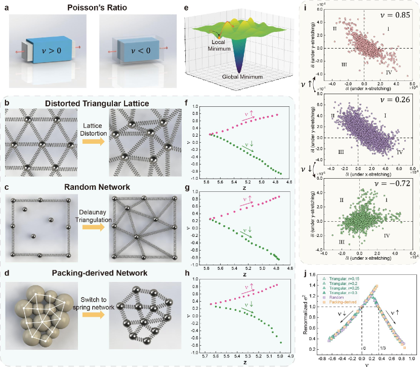
Figure 1: Tuning $\nu$ from positive to negative in three types of amorphous networks. a, a schematics showing the positive and negative $\nu$ behaviors. The red arrows indicate the uniaxial stretching, the original state is drawn in blue, and the deformed state is drawn in light gray. For $\nu>0$, the longitudinal direction elongates while the transverse direction shrinks; for $\nu<0$, both directions elongates. b-d, the construction of three types of amorphous networks: the distorted triangular lattice, the Delaunay-triangulated random network, and the packing-derived network. e, a schematics demonstrating local minimum and global minimum. f-h, tuning towards either positive or negative Poisson’s ratio from the same initial state, for the three types of amorphous networks shown on the left. Note that all configurations throughout tuning contain only convex polygons. i, the statistics of single-bond length changes under stretching. Each data point represents one single bond: its x and y coordinates are the length changes under x and y stretching respectively. The middle panel is the original system, and the top and bottom panels are the systems after $\nu$-increase and $\nu$-decrease tunings respectively. Clearly, systems with positive $\nu$ and negative $\nu$ exhibit distinct data distributions: the former are mostly in quadrants II and IV while the latter are mostly in quadrants I and III. j, the renormalized variance of data points similar to i are plotted against $\nu$, and an excellent collapse for all systems is observed. Note that the left branch of data is renormalized by $\sigma^{2}$ at $\nu=0$, and the right branch of data is renormalized by $\sigma^{2}$ at $\nu=1/3$, as indicated in the plot.

Results

Tuning Poisson’s ratio with simulated annealing algorithm

In our amorphous system, we utilize a network model composed of $N$ nodes connected by $N_{b}$ bonds, where each node has mass $m$, and each bond is an ideal massless spring with the spring constant $k$ [33, 34, 35, 36, 37, 38]. The coordination number $z=2N_{b}/N$ represents the average number of bonds per node [39, 40, 41, 42, 43, 44]. By removing a small fraction of bonds in the network, one can tune the system’s Poisson’s ratio from positive to negative[45, 46, 47] as shown in Figure 1a. To ensure the general validity of this finding, we construct three distinct types of amorphous networks and verify the universality of our results across them. These network types include: (1) the distorted triangular lattice (Figure 1b), (2) the Delaunay-triangulated random network (Figure 1c), and (3) the network derived from packing configurations (Figure 1d) (see Methods for details).

We use the simulated annealing algorithm (see Methods for details), an optimization method (see Figure 1e) that employs an oscillation-like mechanism to escape from local optima solutions, to approach the global optimum. After calculation, we have achieved a tuning range of $-0.9<\nu<0.9$, which approaches the theoretical limit of $-1<\nu<1$ in 2D isotropic systems.To ensure orientation independence, we separately determine $\nu_{x}$ and $\nu_{y}$ under x-stretching and y-stretching, respectively. The average of these values, $\nu=(\nu_{x}+\nu_{y})/2$, represents the system’s overall $\nu$. It is worth noting that, due to the isotropic nature of our system, $\nu_{x}$ and $\nu_{y}$ exhibit similar behavior. As depicted in Figure 1f, g, h, our machine learning algorithm successfully achieves $-0.9<\nu<0.9$ in all three types of amorphous networks, thereby demonstrating its remarkable tuning range and applicability.

To visualize the changes occurring at the single-bond level during the tuning process, we analyze the length changes of each individual bond under $x$-stretching and $y$-stretching. The resulting statistics are presented in Figure 1i: the middle panel depicts the initial configuration, while the upper and lower panels showcase the situations after $\nu$-increase and $\nu$-decrease tunings, respectively. In these plots, each point represents a bond, with its $x$-coordinate and $y$-coordinate indicating the length changes under $x$-stretching and $y$-stretching, respectively. It is evident that the original data points in the middle plot are broadly dispersed across quadrants II and IV, a result of opposite deformation signs due to the positive Poisson’s ratio. However, after either increasing or decreasing $\nu$, the data points converge towards the center, signifying that both types of tuning reduce the extent of bond length changes during stretching, with only a minor fraction undergoing substantial transformations. Intriguingly, tuning $\nu$ to a negative value causes a redistribution of the points into quadrants I and III, in stark contrast to the positive-$\nu$ situations portrayed earlier. Given that quadrants I and III entail $x$ and $y$ deformations with the same sign, this behavior aligns well with the auxetic phenomenon, where both dimensions simultaneously experience expansion or shrinkage.

Hence, Figure 1i clearly illustrates that distinct distribution patterns of bond variations under load correspond to different $\nu$ values. To quantify these patterns, we calculate the variance of each distribution, denoted as $\sigma^{2}={\sum_{i=1}^{N}(\vec{r_{i}}-{\vec{r}_{mean}})^{2}}/{N}$, and renormalize $\sigma^{2}$ to 1 at either $\nu=0$ or $\nu=1/3$ for $\nu$-decrease and $\nu$-increase tunings, respectively. This normalization allows for systematic comparisons across different systems. Surprisingly, when these renormalized $\sigma^{2}$ values are plotted against $\nu$, data from various amorphous systems exhibit excellent collapse onto a master curve, as depicted in Figure 1j. This manifestation indicates a close correlation between the statistical variance of single-bond variations under load, $\sigma^{2}$, and $\nu$. Moreover, our machine learning approach effectively re-distributes $\sigma^{2}$ into quadrants I and III, thereby achieving negative-$\nu$ systems.

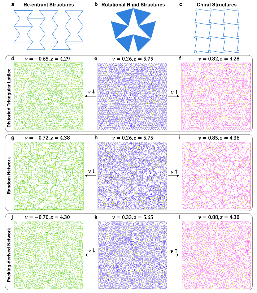
Figure 2: The classical auxetic structures are fundamentally different from the auxetic structures discovered by our machine learning. a-c, The three classical auxetic structures: re-entrant, rotational and chiral structures. d-l, the three rows correspond to the three different amorphous systems. Within each row, the middle panel shows the original structure, and the left and right panels show the negative and more positive configurations found by the machine learning. Apparently, in the left panels of auxetic structures there is no concave and chiral structures typically existing in the classical auxetic structures. Also note that the negative-$\nu$ panels on the left are structurally very similar to the positive-$\nu$ panels on the right with almost a same $z$.

Next, we elucidate the fundamental difference between our auxetic structures and previous designs using Figure 2. In the first row, we showcase three classical auxetic designs: re-entrant [48, 49], rotational [50], and chiral structures [51, 52, 53, 54]. Rows 2 to 4 demonstrate our amorphous networks generated from a distorted triangular lattice (row 2), Delaunay-triangulated random network (row 3), and packing-derived network (row 4). In the middle of each row, we present the original networks with $\nu$ around 0.3, while the highly-negative and highly-positive networks resulting from bond cutting are displayed on the left and right sides, respectively. Notably, our auxetic structures in the left panels differ significantly from the classical designs in the first row: (1) our structures are amorphous and isotropic in all directions, whereas the classical designs exhibit directional-dependent responses; (2) our structures consist entirely of convex polygons; (3) our structures do not possess any chiral characteristics. Additionally, we have conducted computations on varying system sizes, ranging from $12\times 12$ nodes to $32\times 32$ nodes. The results consistently demonstrate the tunability of Poisson’s ratio (see Supplementary Figure 2 and Figure 3). It is evident that regardless of the system size, the Poisson’s ratio converges consistently towards -0.9 for auxetic networks and towards 0.9 for more positive networks. This observation underscores the consistent tunability of our machine learning algorithm across different system dimensions and scales.

Interestingly, the structures with highly negative and highly positive $\nu$ appear quite similar. Both exhibit isotropic structures with similar connectivity (i.e., similar $z$), as depicted in the left panels versus the right panels in Figure 2. However, when subjected to external loading, these visually similar structures exhibit completely opposite Poisson’s ratios. This high structural similarity between structures with positive and negative $\nu$ has not been previously reported, further demonstrating the uniqueness and novelty of the machine learning-generated structures. By combining these visually similar structures, one can also create functionally gradient materials without structural gradient, as illustrated in the Supplementary.

Experimental confirmation of designed amorphous networks

We have successfully achieved continuous tuning of $\nu$ from highly positive to highly negative by employing the machine learning optimization algorithm in general amorphous networks. To validate the simulated annealing algorithm is practical reliable, we experimentally build the networks designed by machine learning and compare their Poisson’s ratio against the numerical prediction. We 3D print amorphous elastomer networks with negative, positive, and zero $\nu$. Note that due to experimental convenience, the 3D printed structures have a smaller system size compared to the simulation structures in Figure 2. However the machine learning protocol used for both the experiment and simulation is exactly the same.

In our experiments, we apply a compression strain of $\varepsilon=-0.1$ to each network. We then measure the corresponding deformation field and Poisson’s ratio using optical imaging. For practical reasons, we only apply compressional strain in the experiment to avoid bond breakage and experimental failure caused by extensional strain. However, we have numerically tested extensional strain and obtained consistent results (see Supplementary for details). To validate the robustness of our design, we test all three types of amorphous networks, which are depicted in the three rows of Figure 3b-j. Remarkably, for each type, we successfully achieve negative, positive, and nearly-zero $\nu$ values. The left panels demonstrate shrinkage or negative $\nu$ in the horizontal response, the right panels show expansion or positive $\nu$, and the middle panels exhibit almost no change or zero $\nu$. The red boxes indicate the initial positions of the systems. The exact deformation process can be observed in Movie-1 to Movie-9. Note that the achieved tuning range is $-0.6<\nu<0.5$, which is narrower than the simulation range of $-0.9<\nu<0.9$. However, this range still confirms that simulated algorithm is quite useful in tuning the Poisson’s ratio. One key reason for this discrepancy is that the simulation assumes a pure spring interaction, whereas the bending effect inevitably exists in actual bonds [55, 56, 57, 58, 59, 60]. Another reason is due to the static friction at the sample’s top and bottom boundaries, which limits the horizontal motion and leads to a reduced tuning range (see Supplementary for more details from simulation). Despite this inherent bending complexity, all amorphous systems demonstrate a significant tuning range, thus highlighting the robustness and general validity of our machine learning design.

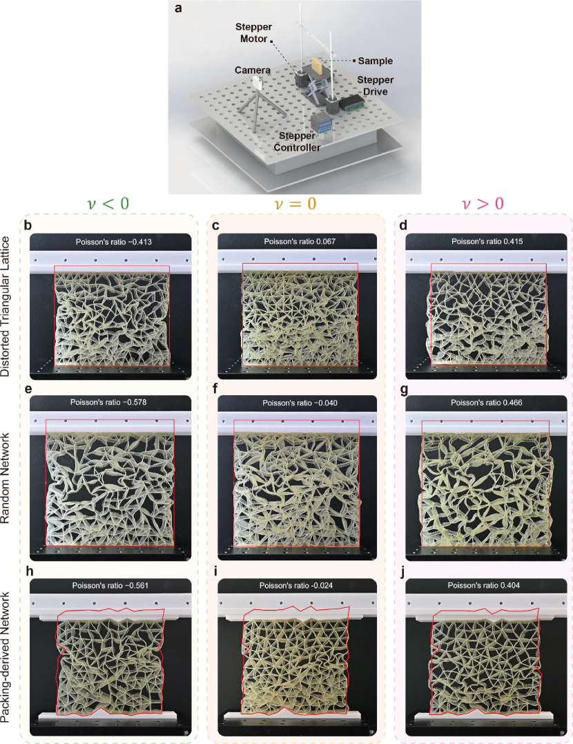
Figure 3: Experimental realization with 3D-printing. a, experimental setup for $\nu$ measurement. The sample is under a compression loading on its top surface driven by two step motors. Compression strain and speed are precisely controlled by the motors. The Poisson’s ratio is measured from the area change of sample during the compression, which is recorded by a camera in front of the sample. b-j, the three rows show the situations of the three amorphous systems. Each snapshot is taken at the compression strain of $\varepsilon=-0.1$, and the red boxes indicate the original boundary without loading. Clearly, the left panels exhibit a negative $\nu$, the middle panels exhibit a nearly-zero $\nu$, and the right panels exhibit a positive $\nu$.

Poisson’s ratio originates from a few normal modes

The fundamental origin that determines $\nu$ remains an open question, which we aim to elucidate using the normal mode picture. In general, we find that only a few low-frequency vibrational normal modes (typically one to two) can determine the Poisson’s ratio of amorphous systems. For a 2D amorphous network with $N$ nodes, we construct a $2N\times 2N$ dynamic matrix and calculate its $2N$ eigenvalues and eigenmodes, corresponding to the vibrational frequencies and normal modes [61, 62, 63, 64, 65]. Across the broad range of $-0.9<\nu<0.9$ and in all our systems, we observe that $\nu$ is universally determined by one to two vibrational normal modes.

To characterize the Poisson’s ratio with normal modes, we define an effective Poisson’s ratio, $\nu^{\prime}$, for each mode. As depicted in Figure 4a and Figure 4b, when we treat the vibrational vectors of a normal mode as displacement vectors on the nodes, the original structure becomes ‘deformed’, resulting in an effective Poisson’s ratio, $\nu^{\prime}$, for that mode. A mode may exhibit either a positive or a negative $\nu^{\prime}$ (see Figure 4a,b). We demonstrate that the actual $\nu$ is determined by the superposition of a few important modes’ $\nu^{\prime}$.

To identify these important modes, we project the actual deformation under load onto all the normal modes, and analyze the projection probabilities or weights. Since normal modes are orthogonal to each other and form an orthonormal set of basis consisting of all $2N$ modes, we can project any actual deformation field onto this set of basis:

$$|\delta r\rangle=\sum_{i=1}^{2N}C_{\omega i}|\omega_{i}\rangle$$ (1)

Here $|\delta r\rangle$ is the actual deformation field under an external load, which is a $2N\times 1$ dimensional vector normalized to unit amplitude. $|\omega_{i}\rangle$ is the $ith$ normal mode with the frequency $\omega_{i}$. $C_{\omega i}=\langle\omega_{i}|\delta r\rangle$ is the projection pre-factor of $|\delta r\rangle$ on mode $|\omega_{i}\rangle$, and $|C_{\omega i}|^{2}$ has the physical meaning of projection probability: it gives the weight or importance of mode $|\omega_{i}\rangle$ in the actual deformation field $|\delta r\rangle$. To obtain a result independent of direction, the external load is applied separately in x and y directions, and the average is obtained as the final projection probability.

Therefore, the importance or weight of each mode in the actual deformation can be illustrated by plotting $|C_{\omega i}|^{2}$ against $\omega_{i}$ in Figure 4c. Notably, two prominent peaks can be observed in the low-frequency range, revealing the significance of two modes, while other modes play a negligible role (note that the weight is zero at high frequencies, and only the low-frequency range is meaningful). Interestingly, these two modes typically exhibit opposite effective Poisson’s ratios $\nu^{\prime}$: one demonstrates a highly positive $\nu^{\prime}$ while the other exhibits a highly negative $\nu^{\prime}$ (denoted as $\omega^{+}$ and $\omega^{-}$ respectively in Figure 3c). By considering their superposition based on their weights, the actual Poisson’s ratio $\nu$ can be determined as $\overline{\nu^{\prime}}=|C_{\omega+}|^{2}\nu^{\prime}(\omega^{+})+|C_{\omega-}|^{2}\nu^{\prime}(\omega^{-})$. This relationship is validated by the linear relation depicted in Figure 4d.

As a result, the origin of $\nu$ essentially originates from the $\nu^{\prime}$ of normal modes. Certain low-frequency modes possess either positive or negative $\nu^{\prime}$. The external load significantly excites one or two such modes. The superposition of these $\nu^{\prime}$ values governs the actual $\nu$ of the system (see Supplementary for a detailed derivation). It is important to note that this mechanism universally applies to all the amorphous systems studied, including the distorted triangular lattice, random network, and packing-derived network. This universality is demonstrated by the excellent data collapse depicted in Figure 4d.

The fundamental origin of $\nu$ from the $\nu^{\prime}$ of normal modes provides a clearer understanding of the tuning process. Figure 4e illustrates how the competition between the two important modes, $\omega^{+}$ and $\omega^{-}$, determines the actual value of $\nu$. When we tune $\nu$ from its original value of 0.3 to a negative value, the importance of $\omega^{-}$ increases, eventually becoming dominant, while the significance of $\omega^{+}$ decreases, becoming negligible. This results in the effective reduction of $\nu$ from a positive to a negative value. Additionally, $\omega^{+}$ and $\omega^{-}$ initially approach each other, then overlap, and finally separate, as depicted in the top to bottom panels. Notably, when these two modes overlap, they exhibit the same height, leading to the cancellation of positive and negative $\nu^{\prime}$. Consequently, a nearly-zero value of $\nu$ is obtained (see panel 3). In contrast, when we tune $\nu$ from its original value of 0.3 to a more positive value, the opposite trend is observed in Figure 4f. The two peaks continue to separate, and the height of $\omega^{+}$ increases while the height of $\omega^{-}$ decreases, eventually becoming negligible. The increasing weight of $\omega^{+}$ contributes to the overall increase in the actual value of $\nu$.

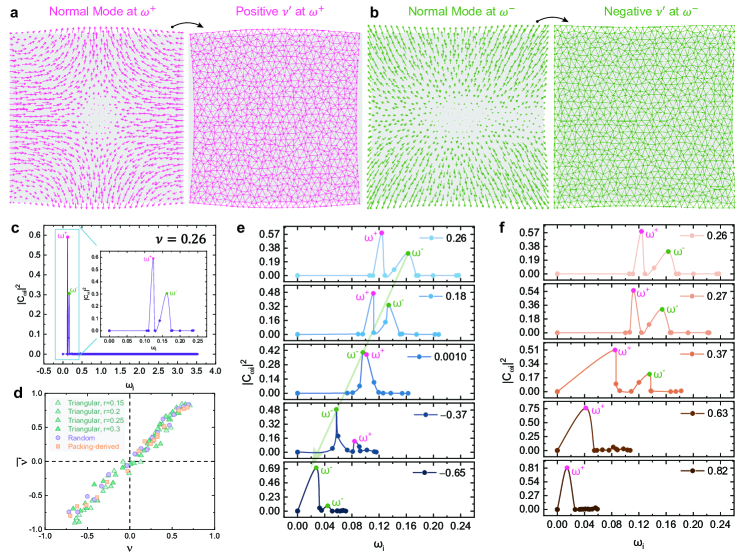
Figure 4: The effective Poisson’s ratio of normal modes, $\nu^{\prime}$, determines the actual $\nu$ of the system. a, the left panel shows the normal mode at the frequency $\omega^{+}$, and the gray area indicates the original state. The right panel shows the configuration after adding the vibrational vectors: clearly the network expands in y direction and shrinks in x direction, which is a typical feature of positive Poisson’s ratio. b, The normal mode at the frequency $\omega^{-}$ shows simultaneous expansion in both x and y directions, which is a typical auxetic behavior. c, $|C_{\omega i}|^{2}$ shows the weight or importance of different normal modes in an actual stretching deformation. Only the low-frequency range is important and the values at high frequencies are all zero. Clearly there are two peaks in the inset: one at $\omega^{+}$ with positive $\nu^{\prime}$ and one at $\omega^{-}$ with negative $\nu^{\prime}$. The superposition of the two $\nu^{\prime}$ based on their weights, $\overline{\nu^{\prime}}=|C_{\omega+}|^{2}\nu^{\prime}(\omega^{+})+|C_{\omega-}|^{2}\nu^{\prime}(\omega^{-})$, determines the actual $\nu$. d, $\overline{\nu^{\prime}}$ from normal modes versus actual $\nu$ shows a nice linear relation, and an excellent data collapse across various systems is observed. Clearly, one to two normal modes can universally determine the actual Poisson’s ratio across various amorphous systems. e, from top to bottom, as $\nu$ is tuned to negative values, the weight of $\omega^{-}$ keeps increasing to dominant while the weight of $\omega^{+}$ keeps decreasing to negligible. When the two modes have similar weights, their $\nu^{\prime}$ cancels out and the system exhibits a nearly-zero $\nu$ (see the middle panel). The positions of two peaks first approach each other, then overlap and eventually separate apart. f, from top to bottom, as $\nu$ is tuned to more positive values, the weight of $\omega^{+}$ keeps increasing to dominant while the weight of $\omega^{-}$ keeps decreasing to negligible. The two peak positions keep separating apart.

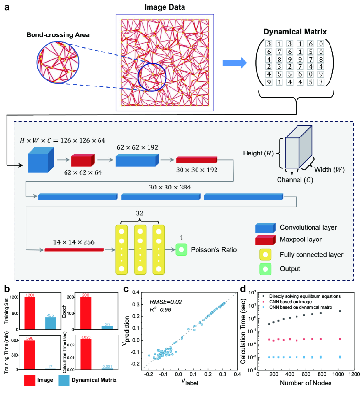
Figure 5: Scientific discovery serves as a catalyst for advancements in deep learning. a, The presence of bond-crossing areas poses challenges for deep learning models, as neural networks struggle to discern whether two crossed bonds share a common node. This challenge is mitigated by substituting images with the dynamical matrix as input, as illustrated by the architecture of AlexNet. b, Comparisons of the training results of CNN models using images and dynamical matrices as inputs. c, Prediction performance of Poisson’s ratio using the dynamical matrix as input from the testing dataset, which the CNN model has never encountered during training. d, Calculation of time cost by directly solving equilibrium equations and CNN models based on images and dynamical matrices. The comparison is conducted across amorphous networks of different sizes, ranging from $12\times 12$ to $32\times 32$.

Scientific discovery drives advancements in deep learning innovation

The underlying mechanism governing the Poisson’s ratio, as revealed by our normal mode analysis, can be effectively utilized to enhance the efficiency and broaden the prediction range of deep learning models. Traditional CNN models rely on image-based training data, which often demand extensive datasets and result in prolonged training time. Moreover, these models may face challenges in situations where image datasets are unsuitable. This is evident in scenarios such as distorting nodes of a triangular lattice to induce auxetic behavior, where multiple bond-crossing areas may emerge, as depicted in Figure 5a. This poses a challenge for CNN models, as they may mistakenly put a node at the crossing point of two bonds whereas there is no node in reality. Analogous to the traditional image input that is a matrix of pixels, we recognize that the mechanical behavior is encoded within network’s dynamical matrix and thus propose to use its dynamical matrix as input to train deep learning models. To demonstrate this concept, we trained the AlexNet model using the dynamical matrix as the training dataset.

The training and prediction performance is further compared with a ResNet-50 model trained using image datasets, as illustrated in Figure 5b-d. Figure 5b highlights that a well-trained network utilizing the dynamical matrix accelerates prediction time by 25 times compared to models using images as inputs. Training with images is notably more challenging, requiring a dataset three times larger and ten times more training epochs, resulting in a training time 35 times longer. As depicted in Figure 5c, the AlexNet demonstrates high accuracy in predicting Poisson’s ratio with the input dynamical matrix, achieving an $R^{2}$ value of $0.98$. The scatter plots closely align around the grey dashed line representing the curve of $\nu_{prediction}=\nu_{label}$. Notably, the prediction range of $\nu$ using images extends from $1/3$ towards 0, which is smaller than the range covered by predictions based on the dynamical matrix, spanning from $1/3$ to $-0.2$. This improvement is due to the characteristics of the dataset components, specifically, the range of node distortions of the triangular lattice for the image training set is smaller than that for the dynamical matrix (refer to the Methods section for details). Consequently, image-based CNN prediction carries inherent and intrinsic limitations compared to the dynamical matrix-based prediction. By uncovering the underlying physics, we can adjust the inputs for CNN models, enabling the prediction of a wide range of Poisson’s ratio values.

Finally, we compare the prediction time of CNN models with input images and input dynamical matrices with the time from solving equilibrium equations, as shown in Figure 5d. Clearly, predictions based on the dynamical matrix are 25 times faster than image-based predictions, and this efficiency remains consistent across amorphous networks with varying numbers of nodes, ranging from 144 to 1024. Increasing the number of nodes amplifies the time cost of solving equations due to the rise in unknown variables. In contrast, the time cost for CNN models remains relatively constant for complex networks with varying numbers of nodes, as their hyperparameters are fixed after training. For the largest-sized amorphous network in our study, the trained AlexNet can make predictions $3.5\times 10^{3}$ times faster than solving equations directly. This underscores the potential revolutionary impact of scientific discovery on the development of deep learning.

Discussion and Conclusion

We have presented a comprehensive research framework, exemplifying the entire “AI for Science” loop. Initially, machine learning algorithms is employed to generate the database for unveiling the underlying physical mechanism of Poisson’s ratio. Subsequently, experimental validation has confirmed the designed auxetic performance of amorphous materials from machine learning. Furthermore, we leverage the physical mechanism to improve deep learning models from dynamical matrix instead of image input. Note that the structures generated by our machine learning algorithm deviate significantly from previous designs, which is the crucial prerequisite for discovering novel and fundamental physical mechanisms. Traditional designs for auxetic networks relied on periodically arranged unit cells and concave structures. By contrast, our machine learning-generated structures exclusively consist of convex structures which produces a completely new design paradigm. This unique structural approach enables further exploration into the underlying mechanism of Poisson’s ratio. Through normal mode analysis, we unveil that a subset of low-frequency normal modes of the dynamical matrix determines Poisson’s ratio.

Given that deep learning typically relies on image datasets represented as matrices encoding RGB channel pixels, we use deep neural networks to extract mechanical properties encoded within the dynamical matrix. Additionally, traditional image-based dataset acquisition can be time-consuming and resource-intensive, making it less suitable for certain scientific inquiries. By replacing images with physical descriptors, such as the dynamical matrix, we can gain a significant efficiency advantage. This approach reduces the input training data size, as each sample now only consists of a single-channel dynamical matrix. Consequently, the training time required for a CNN model is significantly reduced. This trained CNN effectively serves as a surrogate model to avoid extensive calculations on actual systems. This breakthrough illuminates a promising pathway that bridges the gap between artificial intelligence and fundamental scientific research. Importantly, it highlights the dual role of AI, not only providing sufficient data for fundamental research but also driving the development of AI through fundamental mechanisms obtained from AI-produced data.

Methods

Construction of the amorphous networks

As illustrated in the left panel of Figure 1b in the main text, the intiial network is a perfect triangular lattice. To introduce distortion, we apply a displacement vector to each node inside the boundary, as shown in the right panel of the figure. The displacement vector of the $\alpha$th node is denoted as $\delta\vec{r_{\alpha}}=(r\cos{\theta_{\alpha}},r\sin{\theta_{\alpha}})$, where $\theta_{\alpha}$ is randomly distributed in the range $[0,2\pi]$ and represents the direction of displacement, and $r$ represents the degree of distortion. It is important to note that $r$ should be less than half the lattice constant to avoid bond crossings. After the distortion, the connections between nodes are replaced with new relaxed springs.

Figure 1c in the main text illustrates the process of constructing a random network. In the left panel, a set of nodes (represented as balls) is randomly distributed within a rectangular region. The right panel of the figure shows the creation of bonds (relaxed springs) through Delaunay triangulation, ensuring that the mean coordination number of the amorphous network, denoted as $<z>$, is set to 6.

As shown in the left panel of Figure 1d in the main text, the network depicted is derived from a typical two-dimensional bi-dispersion packing system. This packing system consists of two types of particles with the same number, and their radius ratio is $1:1.4$. In the next step, the particles are replaced by identical balls, and the contacts between neighboring particles are substituted with identical relaxed springs, as illustrated in the right panel.

Simulated Annealing (SA) Method

Using machine learning, we first illustrate a general and effective tuning approach for $\nu$. Although in previous studies $\nu$ can be tuned to negative in packing-derived networks [45, 29], a general tuning approach for an arbitrary amorphous network is still lacking. Moreover, the previous bond-cutting procedure is based on the importance of a single bond to $\nu$, which typically leads to a locally-optimized result instead of the globally-optimized result (see Figure 1e). Thus the tuning range or efficiency is rather limited. How to approach the globally-optimized result? We tackle this problem with the machine learning algorithms developed in reinforcement learning [66]. Such algorithms have a feedback mechanism which modifies the optimization strategies, and allows the algorithms to accept undesirable results to ‘jump’ out of the local minimum. Eventually the system will approach the global minimum which traps the system much better. After generating a large number of globally-optimized networks, the data set is then fed back to the actual network to get the best bond-cutting procedure for $\nu$ adjustment.

The simulated annealing (SA) algorithm is a widely used optimization method that mimics the gradual cooling process observed in metals. In each iteration, corresponding to an annealing temperature, the algorithm generates a new potential solution by modifying the current state. The new state is then accepted or rejected based on the Metropolis criteria, and this process continues until convergence. The SA algorithm is known for its ability to avoid local optima and approach the global optimal solution. In each iteration, a certain number of bonds are either removed or added to the system, causing a change in the system’s Poisson’s ratio from $\nu(\pi_{t})$ to $\nu(\pi_{t+1})$, where $\pi_{t}$ and $\pi_{t+1}$ represent the network structures at steps $t$ and $t+1$. The algorithm consists of an external loop and an internal loop. The annealing process is applied in the external loop, where the system starts with an initial temperature $T_{0}$ and cools down to the next step $T_{t+1}=\alpha T_{t}$ with a cooling rate $\alpha$. The annealing process terminates when the system reaches its final temperature $T_{f}$. The internal loop involves the implementation of the Metropolis principle. At each discrete temperature $T_{t}$, we iterate $L_{k}$ times in order to find the optimal solution by adjusting the system’s bonds. Here, $L_{k}$ represents the length of the Markov chain. In the internal loop, we introduce an acceptance probability $P$, analogous to the transition matrix used in the Markov Chain Monte Carlo (MCMC) algorithm, to facilitate the system in escaping local optima and approaching global optima.

Next, we demonstrate how the SA algorithm functions using an example of $\nu$-decreasing. After removing specific bonds, the network structure changes from $\pi_{t}$ to $\pi_{t+1}$. The acceptance probability $P$ can be represented by the following expression, which depends on the difference between $\nu(\pi_{t})$ and $\nu(\pi_{t+1})$:

$$P=\begin{cases}1,&\text{if }\nu(\pi_{t+1})<\nu(\pi_{t});\\ e^{(-\dfrac{{\nu(\pi_{t+1})-\nu(\pi_{t})}}{{T_{t}}})},&\text{if }\nu(\pi_{t+1})>\nu(\pi_{t}).\end{cases}$$ (2)

Accordingly, if there is a decrease in $\nu$ after one iteration step, the operation is accepted without question ($P=1$). Conversely, if $\nu$ increases, the algorithm considers accepting the bonds cutting strategy based on the Metropolis principle. It generates a random number $\epsilon$ within the range of [0,1] and compares it with the exponential function $P$. If $\epsilon\leq P$, the strategy is accepted. Otherwise, the algorithm proceeds to the next iteration.

Visualizing the solution space as a landscape, the optimal bond cutting strategy can be considered as a ball falling into a pit. The aim of finding the globally optimal strategy is to guide the ball to find the deepest pit in the landscape. However, without a reliable algorithm, the ball may become trapped in local minima, as depicted in Figure 1e in the main text. To address this issue, the SA algorithm implements a dynamic acceptance probability determined by the temperature $T_{t}$ at time $t$ and the difference in Poisson’s ratio between two consecutive states, $\Delta\nu=\nu(\pi_{t+1})-\nu(\pi_{t})$. By employing this dynamic acceptance probability and the Metropolis principle, the solution space is effectively stirred. This helps the ball to move out of the local minima and continue exploring the solution space until it eventually reaches the globally deepest pit. Once the ball reaches the deepest pit, it is very difficult to move out and has to stay. Similarly, for an increase in $\nu$, the acceptance probability $P$ for a bad strategy becomes $\exp(-(\nu(\pi_{t+1})-\nu(\pi_{t}))/T_{t})$ if $\nu(\pi_{t+1})<\nu(\pi_{t})$.

Prediction of Poisson’s ratio through deep learning

The CPU utilized in our study is the Intel(R) Core(TM) i7-10700, complemented by the NVIDIA GeForce GTX 1650 GPU. We employed triangular networks with varying distortion radii to train the Convolutional Neural Network. The training dataset for AlexNet, with the dynamical matrix as input, covered distortion radii ranging from 0.05 to 0.95 in the triangular lattice. This range produced a diverse set of network Poisson’s ratio values, spanning from $1/3$ to around $-0.2$.

It is noteworthy that lattice distortions exceeding 0.45 can induce auxetic behavior while introducing a cross-bond pattern, presenting challenges for computer vision tasks in discerning whether intersecting bonds share a common node. However, when generating the image dataset, the node distortion radius was constrained to the range of 0.05 to 0.45. This range, notably smaller than the dynamical matrix dataset, was deliberately chosen to avoid bond-crossing areas in images. Consequently, image-based training inherently comes with a limitation, offering a smaller prediction range for Poisson’s ratio. Due to the intricacies involved in image recognition, the accurate prediction requires deeper-layered neural networks. Therefore, we chose the ResNet-50 model for training with image-based datasets, as it is well-suited for handling complex datasets and can alleviate the vanishing/exploding gradient issue.

The dataset was partitioned into training, validation, and testing sets at a ratio of 6:2:2. For feature extraction in AlexNet, we employed five convolutional layers followed by three pooling layers for dimension reduction. This sequential process facilitated the extraction of essential information at each layer, culminating in the final pooling layer. The resulting feature map was flattened into a one-dimensional neural network, connected to two additional fully connected layers. In the context of our prediction task, the output layer consisted of a single neuron responsible for regressing the value of Poisson’s ratio. The well-trained neural network served as a surrogate model, obviating the need for matrix solving and enabling the prediction of Poisson’s ratio for the given network. Post-training, we utilized the neural network to predict the Poisson’s ratio for previously unseen samples constituting a separate dataset known as the testing set. The predictive performance of the optimal trained model can be quantitatively evaluated by the testing dataset with two metrics, i.e., root mean square error ($RMSE$) and determination coefficient ($R^{2}$) defined by: $RMSE=\sqrt{\frac{1}{N}\sum_{i=1}^{N}(\hat{\nu}_{i}-\nu_{i})^{2}}$, $R^{2}=1-\frac{\sum_{i=1}^{N}(\hat{\nu}_{i}-\nu_{i})^{2}}{\sum_{i=1}^{N}(\bar{\nu}_{i}-\nu_{i})^{2}}$, where $\bar{\nu}_{i}$ denotes the average value of testing dataset, while $\nu_{i}$ and $\hat{\nu}_{i}$ denote the predicted and label Poisson’s ratio values.

Acknowledgements L. X. acknowledges the financial support from NSFC-12074325, GRF-14307721, CRF-C6016-20G, CRF-C1018-17G, CUHK direct grant 4053582, X. S. acknowledges the financial support from NSFC, under the Grant No. 12205138, from Shenzhen Science and Technology Innovation Committee (SZSTI), under the Grant No. JCYJ20220530113206015.

Author contributions C. Z. performed all the machine learning computations and experiments, C. Z., X. S. and L. X. contributed to the theoretical normal mode analysis, C. F., Z. J. and B. L. helped in the experiment or the data analysis, C. Z., X. S. and L. X. prepared the manuscript, X. S. and L. X. conceived and supervised the research.

Competing interests The authors declare no competing financial interests.

Data and materials availability All data are available in the main text or the Supplementary Information.

Code availability All custom computer code or algorithm used to generate results that are reported in the paper are available upon request.

Correspondence and requests for materials should be addressed to L. X. (xuleixu@cuhk.edu.hk) and X. S. (shenxy@sustech.edu.cn).

References

- [1] Hanchen Wang, Tianfan Fu, Yuanqi Du, Wenhao Gao, Kexin Huang, Ziming Liu, Payal Chandak, Shengchao Liu, Peter Van Katwyk, Andreea Deac, et al. Scientific discovery in the age of artificial intelligence. Nature, 620(7972):47–60, 2023.
- [2] Jonathan M Stokes, Kevin Yang, Kyle Swanson, Wengong Jin, Andres Cubillos-Ruiz, Nina M Donghia, Craig R MacNair, Shawn French, Lindsey A Carfrae, Zohar Bloom-Ackermann, et al. A deep learning approach to antibiotic discovery. Cell, 180(4):688–702, 2020.
- [3] Vahe Tshitoyan, John Dagdelen, Leigh Weston, Alexander Dunn, Ziqin Rong, Olga Kononova, Kristin A Persson, Gerbrand Ceder, and Anubhav Jain. Unsupervised word embeddings capture latent knowledge from materials science literature. Nature, 571(7763):95–98, 2019.
- [4] Yann LeCun, Yoshua Bengio, and Geoffrey Hinton. Deep learning. nature, 521(7553):436–444, 2015.
- [5] Marc G Bellemare, Salvatore Candido, Pablo Samuel Castro, Jun Gong, Marlos C Machado, Subhodeep Moitra, Sameera S Ponda, and Ziyu Wang. Autonomous navigation of stratospheric balloons using reinforcement learning. Nature, 588(7836):77–82, 2020.
- [6] Kevin Tran and Zachary W Ulissi. Active learning across intermetallics to guide discovery of electrocatalysts for co2 reduction and h2 evolution. Nature Catalysis, 1(9):696–703, 2018.
- [7] Kevin Maik Jablonka, Giriprasad Melpatti Jothiappan, Shefang Wang, Berend Smit, and Brian Yoo. Bias free multiobjective active learning for materials design and discovery. Nature communications, 12(1):2312, 2021.
- [8] Georgia Karagiorgi, Gregor Kasieczka, Scott Kravitz, Benjamin Nachman, and David Shih. Machine learning in the search for new fundamental physics. Nature Reviews Physics, 4(6):399–412, 2022.
- [9] Ekaterina Govorkova, Ema Puljak, Thea Aarrestad, Thomas James, Vladimir Loncar, Maurizio Pierini, Adrian Alan Pol, Nicolò Ghielmetti, Maksymilian Graczyk, Sioni Summers, et al. Autoencoders on field-programmable gate arrays for real-time, unsupervised new physics detection at 40 mhz at the large hadron collider. Nature Machine Intelligence, 4(2):154–161, 2022.
- [10] Matthew D Witman, Anuj Goyal, Tadashi Ogitsu, Anthony H McDaniel, and Stephan Lany. Defect graph neural networks for materials discovery in high-temperature clean-energy applications. Nature Computational Science, pages 1–12, 2023.
- [11] Levi H Dudte, Gary PT Choi, Kaitlyn P Becker, and L Mahadevan. An additive framework for kirigami design. Nature Computational Science, 3(5):443–454, 2023.
- [12] Cen Wan and David T Jones. Protein function prediction is improved by creating synthetic feature samples with generative adversarial networks. Nature Machine Intelligence, 2(9):540–550, 2020.
- [13] Kevin K Yang, Zachary Wu, and Frances H Arnold. Machine-learning-guided directed evolution for protein engineering. Nature methods, 16(8):687–694, 2019.
- [14] Maciej Majewski, Adrià Pérez, Philipp Thölke, Stefan Doerr, Nicholas E Charron, Toni Giorgino, Brooke E Husic, Cecilia Clementi, Frank Noé, and Gianni De Fabritiis. Machine learning coarse-grained potentials of protein thermodynamics. Nature Communications, 14(1):5739, 2023.
- [15] Sergio Pablo-García, Santiago Morandi, Rodrigo A Vargas-Hernández, Kjell Jorner, Žarko Ivković, Núria López, and Alán Aspuru-Guzik. Fast evaluation of the adsorption energy of organic molecules on metals via graph neural networks. Nature Computational Science, pages 1–10, 2023.
- [16] Prabudhya Roy Chowdhury, Colleen Reynolds, Adam Garrett, Tianli Feng, Shashishekar P Adiga, and Xiulin Ruan. Machine learning maximized anderson localization of phonons in aperiodic superlattices. Nano Energy, 69:104428, 2020.
- [17] Han Wei, Hua Bao, and Xiulin Ruan. Genetic algorithm-driven discovery of unexpected thermal conductivity enhancement by disorder. Nano Energy, 71:104619, 2020.
- [18] Jaeman Song, Minwoo Choi, Zhimin Yang, Jungchul Lee, and Bong Jae Lee. A multi-junction-based near-field solar thermophotovoltaic system with a graphite intermediate structure. Applied Physics Letters, 121(16), 2022.
- [19] Run Hu, Sotaro Iwamoto, Lei Feng, Shenghong Ju, Shiqian Hu, Masato Ohnishi, Naomi Nagai, Kazuhiko Hirakawa, and Junichiro Shiomi. Machine-learning-optimized aperiodic superlattice minimizes coherent phonon heat conduction. Physical Review X, 10(2):021050, 2020.
- [20] Shenghong Ju, Takuma Shiga, Lei Feng, Zhufeng Hou, Koji Tsuda, and Junichiro Shiomi. Designing nanostructures for phonon transport via bayesian optimization. Physical Review X, 7(2):021024, 2017.
- [21] Zoubin Ghahramani. Probabilistic machine learning and artificial intelligence. Nature, 521(7553):452–459, 2015.
- [22] Victor Fung, Guoxiang Hu, Panchapakesan Ganesh, and Bobby G Sumpter. Machine learned features from density of states for accurate adsorption energy prediction. Nature communications, 12(1):88, 2021.
- [23] Masashi Tsubaki and Teruyasu Mizoguchi. Quantum deep field: data-driven wave function, electron density generation, and atomization energy prediction and extrapolation with machine learning. Physical Review Letters, 125(20):206401, 2020.
- [24] Yiwei Liu, Cheng Zhang, Zhonghua Liu, Donald G Truhlar, Ying Wang, and Xiao He. Supervised learning of a chemistry functional with damped dispersion. Nature Computational Science, 3(1):48–58, 2023.
- [25] Logan Ward and Chris Wolverton. Atomistic calculations and materials informatics: A review. Current Opinion in Solid State and Materials Science, 21(3):167–176, 2017.
- [26] Jonathan Schmidt, Mário RG Marques, Silvana Botti, and Miguel AL Marques. Recent advances and applications of machine learning in solid-state materials science. npj Computational Materials, 5(1):83, 2019.
- [27] Jakub Kubečka, Yosef Knattrup, Morten Engsvang, Andreas Buchgraitz Jensen, Daniel Ayoubi, Haide Wu, Ove Christiansen, and Jonas Elm. Current and future machine learning approaches for modeling atmospheric cluster formation. Nature Computational Science, 3(6):495–503, 2023.
- [28] Roderic Lakes. Foam structures with a negative poisson’s ratio. Science, 235(4792):1038–1040, 1987.
- [29] Daniel Hexner, Andrea J Liu, and Sidney R Nagel. Role of local response in manipulating the elastic properties of disordered solids by bond removal. Soft matter, 14(2):312–318, 2018.
- [30] Jun Liu, Yunhuan Nie, Hua Tong, and Ning Xu. Realizing negative poisson’s ratio in spring networks with close-packed lattice geometries. Physical Review Materials, 3(5):055607, 2019.
- [31] Alessio Zaccone and Eugene M Terentjev. Short-range correlations control the g/k and poisson ratios of amorphous solids and metallic glasses. Journal of Applied Physics, 115(3), 2014.
- [32] M Schlegel, J Brujic, EM Terentjev, and A Zaccone. Local structure controls the nonaffine shear and bulk moduli of disordered solids. Scientific reports, 6(1):18724, 2016.
- [33] Xiaoming Mao and Tom C Lubensky. Maxwell lattices and topological mechanics. Annual Review of Condensed Matter Physics, 9:413–433, 2018.
- [34] TC Lubensky, CL Kane, Xiaoming Mao, Anton Souslov, and Kai Sun. Phonons and elasticity in critically coordinated lattices. Reports on Progress in Physics, 78(7):073901, 2015.
- [35] Zexin Zhang, Ning Xu, Daniel TN Chen, Peter Yunker, Ahmed M Alsayed, Kevin B Aptowicz, Piotr Habdas, Andrea J Liu, Sidney R Nagel, and Arjun G Yodh. Thermal vestige of the zero-temperature jamming transition. Nature, 459(7244):230–233, 2009.
- [36] Anton Souslov, Andrea J Liu, and Tom C Lubensky. Elasticity and response in nearly isostatic periodic lattices. Physical review letters, 103(20):205503, 2009.
- [37] Natalia Lera, JV Alvarez, and Kai Sun. Topological mechanical metamaterial with nonrectilinear constraints. Physical Review B, 98(1):014101, 2018.
- [38] Yunhuan Nie, Hua Tong, Jun Liu, Mengjie Zu, and Ning Xu. Role of disorder in determining the vibrational properties of mass-spring networks. Frontiers of Physics, 12(3):1–11, 2017.
- [39] D Zeb Rocklin, Lilian Hsiao, Megan Szakasits, Michael J Solomon, and Xiaoming Mao. Elasticity of colloidal gels: structural heterogeneity, floppy modes, and rigidity. Soft Matter, 17(29):6929–6934, 2021.
- [40] Di Zhou, Leyou Zhang, and Xiaoming Mao. Topological boundary floppy modes in quasicrystals. Physical Review X, 9(2):021054, 2019.
- [41] D Rocklin, Shangnan Zhou, Kai Sun, and Xiaoming Mao. Transformable topological mechanical metamaterials. Nature communications, 8(1):1–9, 2017.
- [42] D Zeb Rocklin, Bryan Gin-ge Chen, Martin Falk, Vincenzo Vitelli, and TC Lubensky. Mechanical weyl modes in topological maxwell lattices. Physical review letters, 116(13):135503, 2016.
- [43] M Wyart, H Liang, A Kabla, and L Mahadevan. Elasticity of floppy and stiff random networks. Physical review letters, 101(21):215501, 2008.
- [44] Alessio Zaccone and Enzo Scossa-Romano. Approximate analytical description of the nonaffine response of amorphous solids. Physical Review B, 83(18):184205, 2011.
- [45] Carl P Goodrich, Andrea J Liu, and Sidney R Nagel. The principle of independent bond-level response: Tuning by pruning to exploit disorder for global behavior. Physical review letters, 114(22):225501, 2015.
- [46] Xiangying Shen, Chenchao Fang, Zhipeng Jin, Hua Tong, Shixiang Tang, Hongchuan Shen, Ning Xu, Jack Hau Yung Lo, Xinliang Xu, and Lei Xu. Achieving adjustable elasticity with non-affine to affine transition. Nature Materials, 20(12):1635–1642, 2021.
- [47] Zhipeng Jin, Chenchao Fang, Xiangying Shen, and Lei Xu. Designing amorphous networks with adjustable poisson ratio from a simple triangular lattice. Phys. Rev. Appl., 18:054052, Nov 2022.
- [48] Kenneth E Evans, MA Nkansah, IJ Hutchinson, and SC Rogers. Molecular network design. Nature, 353(6340):124–124, 1991.
- [49] Stefan Bronder, Franziska Herter, Anabel Röhrig, Dirk Bähre, and Anne Jung. Design study for multifunctional 3d re-entrant auxetics. Advanced Engineering Materials, 24(1):2100816, 2022.
- [50] A Alderson and KE Evans. Rotation and dilation deformation mechanisms for auxetic behaviour in the -cristobalite tetrahedral framework structure. Physics and Chemistry of Minerals, 28(10):711–718, 2001.
- [51] Tobias Frenzel, Muamer Kadic, and Martin Wegener. Three-dimensional mechanical metamaterials with a twist. Science, 358(6366):1072–1074, 2017.
- [52] Hsin-Haou Huang, Bao-Leng Wong, and Yen-Chang Chou. Design and properties of 3d-printed chiral auxetic metamaterials by reconfigurable connections. physica status solidi (b), 253(8):1557–1564, 2016.
- [53] Chan Soo Ha, Michael E Plesha, and Roderic S Lakes. Chiral three-dimensional lattices with tunable poisson’s ratio. Smart Materials and Structures, 25(5):054005, 2016.
- [54] D Prall and RS Lakes. Properties of a chiral honeycomb with a poisson’s ratio of—1. International Journal of Mechanical Sciences, 39(3):305–314, 1997.
- [55] Jingchen Feng, Herbert Levine, Xiaoming Mao, and Leonard M Sander. Nonlinear elasticity of disordered fiber networks. Soft matter, 12(5):1419–1424, 2016.
- [56] Daniel R Reid, Nidhi Pashine, Justin M Wozniak, Heinrich M Jaeger, Andrea J Liu, Sidney R Nagel, and Juan J de Pablo. Auxetic metamaterials from disordered networks. Proceedings of the National Academy of Sciences, 115(7):E1384–E1390, 2018.
- [57] Jason W Rocks, Nidhi Pashine, Irmgard Bischofberger, Carl P Goodrich, Andrea J Liu, and Sidney R Nagel. Designing allostery-inspired response in mechanical networks. Proceedings of the National Academy of Sciences, 114(10):2520–2525, 2017.
- [58] Chase P Broedersz, Xiaoming Mao, Tom C Lubensky, and Frederick C MacKintosh. Criticality and isostaticity in fibre networks. Nature Physics, 7(12):983–988, 2011.
- [59] Daniel R Reid, Nidhi Pashine, Alec S Bowen, Sidney R Nagel, and Juan J de Pablo. Ideal isotropic auxetic networks from random networks. Soft Matter, 15(40):8084–8091, 2019.
- [60] D Zeb Rocklin and Xiaoming Mao. Self-assembly of three-dimensional open structures using patchy colloidal particles. Soft Matter, 10(38):7569–7576, 2014.
- [61] Xiaoming Mao, Ning Xu, and TC Lubensky. Soft modes and elasticity of nearly isostatic lattices: Randomness and dissipation. Physical review letters, 104(8):085504, 2010.
- [62] Katia Bertoldi, Vincenzo Vitelli, Johan Christensen, and Martin Van Hecke. Flexible mechanical metamaterials. Nature Reviews Materials, 2(11):1–11, 2017.
- [63] Ling-Nan Zou, Xiang Cheng, Mark L Rivers, Heinrich M Jaeger, and Sidney R Nagel. The packing of granular polymer chains. Science, 326(5951):408–410, 2009.
- [64] Sean A Ridout, Jason W Rocks, and Andrea J Liu. Correlation of plastic events with local structure in jammed packings across spatial dimensions. Proceedings of the National Academy of Sciences, 119(16):e2119006119, 2022.
- [65] Hideyuki Mizuno, Kuniyasu Saitoh, and Leonardo E Silbert. Elastic moduli and vibrational modes in jammed particulate packings. Physical Review E, 93(6):062905, 2016.
- [66] Scott Kirkpatrick, C Daniel Gelatt Jr, and Mario P Vecchi. Optimization by simulated annealing. Science, 220(4598):671–680, 1983.