Multiple wave packets running in the photon number-space
Abstract
If a two-level system coupled to a single-mode cavity is strongly driven by an external laser, instead of a continuous accumulation of photons in the cavity, oscillations in the mean photon number occur. These oscillations correspond to peaks of finite width running up and down in the photon number distribution, reminiscent of wave packets in linear chain models. A single wave packet is found if the cavity is resonant to the external laser. Here, we show that for finite detuning multiple packet structures can exist simultaneously, oscillating at different frequencies and amplitudes. We further study the influence of dissipative effects resulting in the formation of a stationary state, which depending on the parameters can be characterized by a bimodal photon number distribution. While we give analytical limits for the maximally achievable photon number in the absence of any dissipation, surprisingly, dephasing processes can push the photon occupations towards higher photon numbers.
I Introduction
Ever since the dawn of quantum theory, there has been a strive towards controlling the quantum states of various matter systems such as atoms or molecules [1, 2, 3, 4, 5, 6, 7, 8]. Their interaction with electromagnetic fields is commonly used as a lever to achieve this goal. More recently, control of the quantum state of light itself has attracted much attention, where now the matter systems take on the supportive role [9, 10, 11, 12, 13, 14]. With the methods of cavity quantum electrodynamics (cQED), nonclassical photonic states can be deliberately generated, including but not limited to Fock states [15, 16, 17, 18, 19, 20, 21], squeezed states [22, 23, 24, 25, 26] and Schrödinger cat states [27, 28, 29, 30, 31]. Besides the fundamental interest in nonclassical states as manifestations of the intricacies of quantum physics, they offer perspectives for technological advancements, e.g. through the use of in principle unlimited degrees of freedom to encode information [32, 33, 34, 35, 36, 37, 38, 39, 40].
In this work, we focus on the simplest model providing a platform to study cQED, namely a two-level system (TLS) coupled to a single-mode microcavity. This model is capable of capturing the central features of a large variety of real systems, such as atoms, semiconductor quantum dots, or superconducting qubits. Each realization is understood as sampling different regions of the parameter space [41].
We investigate novel highly nonclassical states that are characterized by multiple peaks in the photon number distribution, each of which constituting the center of a structure of finite width, which we will call a packet. They exhibit rich dynamics with each peak oscillating at different frequencies and amplitudes. We show that these states can be produced in simple fashion via strong continuous wave (cw) driving of the TLS. As the result of dissipation, a stationary state will form after some time, which describes a similar bimodal distribution under the right circumstances. The characteristics of both the dynamical behavior as well as the stationary state can be easily controlled by varying the driving strength and detuning the frequency of the external driving with respect to the resonance frequency of the cavity. In addition, we discuss a remarkable mechanism that allows for occupation of photon numbers higher than in equivalent conservative systems if the dephasing of the TLS dominates the losses of the cavity.
II Theoretical model
The TLS-cavity system is described by a Jaynes–Cummings model. The Hamiltonian in the interaction picture with respect to the driving frequency reads
| (1) |
The ground state of the TLS is chosen as a state of energy zero, whereas the excited state has energy . and are the detunings between the external driving and the TLS and cavity respectively, where is the frequency of the cavity-mode. The constant denotes the coupling strength between TLS and cavity, while is the external driving strength. () is the familiar photonic annihilation (creation) operator; and denote the ladder operators of the TLS satisfying fermionic anticommutation relations. The basis of product states , named the bare state basis, spans the Hilbert space of the combined system, where is the Fock state with photon number . For simplicity’s sake we consider only cases of a resonantly driven TLS . Numerical studies indicate, that a finite value of does not noticeably change the results discussed in this work. However, the novel phenomena that we shall present in this paper appear only for finite laser–cavity detuning. We therefore have to allow for a finite .
As long as no dissipative effects are considered, we integrate the Schrödinger equation
| (2) |
expanding the wave function in the bare state basis, by using a classic Runge-Kutta method (RK4). Unless otherwise mentioned, the initial state is taken as the ground state without photons .
In Sec. V we present the behavior of the system under the influence of different dissipative effects. All of them are assumed to be well-approximated as Markov processes, so that the dynamical evolution of the density matrix can be calculated as the solution to the Liouville-von Neumann equation
| (3) |
where the superoperators , and are of Lindblad form
| (4a) | ||||
| (4b) | ||||
| (4c) | ||||
These terms model losses of the cavity, radiative decay and pure dephasing of the TLS, respectively. We solve Eq. (II) similar to Eq. (2) by expanding the density matrix in the bare state basis and integrating the resulting system of differential equations by application of RK4.
III Numerical results
In order to obtain a clear picture of the dynamical behavior, we first investigate the solutions without any dissipation. As will be shown in Sec. V, the same dynamical characteristics will be present transiently when dissipation is taken into account.
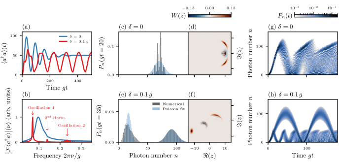
In Fig. 1(a) the time-resolved mean photon number is shown in both a resonant () and a non-resonant case (). In the former, a harmonic damped oscillation can be seen. Accordingly, its Fourier transform [cf. Fig. 1(b)] consists of a single broad peak. Due to the well-known collapse-and-revival effect [42], the oscillation will reappear after some time (not shown in Figs. 1(a) and (b)). We emphasize that the photon number will never exceed a finite maximal value even without dissipation. This is remarkable since the system is continuously driven enabling an energy flow between the TLS and the laser. Furthermore in the driven system all of the infinite steps of the Jaynes–Cummings ladder are coupled.
For finite but small detuning , a significantly different behavior is found. The most prominent oscillation frequency is shifted with respect to that of while the corresponding peak is of much lower spectral width. Hence, the decay of the oscillation is only visible on a longer time scale. In addition to small peaks at the second and third harmonic of this oscillation, contributions at a second higher fundamental frequency appear [cf. Fig. 1(b)]. Since it does not coincide with an integer multiple of the first frequency, this fact indicates the presence of two separate oscillating structures.
The photon number distribution
| (5) |
shown at fixed time in Fig. 1(c) for and Fig. 1(e) for , reveals the two frequencies to correspond to two separate packets that oscillate independently from each other. In contrast, only a single packet is present for consistent with the single oscillation frequency of the mean photon number. This is also in line with Ref. [42] where starting from the analytical solution, which is only available for and without dissipation, a single oscillation of the mean photon number was approximately derived.
Distributions with multiple peaks obviously correspond to highly nonclassical states. Yet, in some cases even the packets themselves can be classified as such, which can be shown by comparing them to best fits of Poisson distributions to the peak structures or identifying regions of negative values in the Wigner function [43]
| (6) |
Here, denotes the photonic density matrix and is the displacement operator. Both the single packet in the resonant case as well as the packet of lower photon number in the detuned case clearly exhibit these characteristics of nonclassicality, whereas the packet of higher photon number is more akin to a coherent state [cf. Figs. 1(d) and 1(f)].
Figs. 1(g) and 1(h) visualize the time-dependence of itself. For , the initially present packet quickly disperses in agreement with the collapse of the oscillation of the mean photon number in Fig. 1(a). Similar behavior is exhibited for by the packet of lower oscillation amplitude, which incidentally corresponds to a higher oscillation frequency. The packet of higher photon number shows a stable propagation for much longer times, providing further evidence that it behaves in a similar fashion to a single harmonic oscillator. Indeed, this structure remains stable for more than 20 oscillation cycles for the particular set of parameters given in Fig. 1(h).

IV Analytical results for strong driving
With the aim of gaining qualitative understanding of the dynamics, we analyze the situation of a strongly driven TLS. Here, we concentrate on limiting cases where analytical results can be found. We assume a cavity that is only slightly detuned, such that the hierarchy holds.
IV.1 Low excitation numbers
Since constitutes the dominant energy scale, it is natural to attempt a description in terms of the laser-dressed states (LDS)
| (7) |
which diagonalise the driving operator . The energies of the corresponding product states are given by . Via cavity coupling, transitions between states of neighboring photon numbers are induced, both at unchanged LDS as well as accompanying a transition , as sketched in Fig. 2(a). The absolute values of the corresponding matrix elements are .
At the beginning of the dynamics and also after completion of a cycle in an oscillation of a packet only states with small photon numbers are occupied. We concentrate on the regime where the following inequality holds for all occupied states with photon number in a given packet:
| (8) |
In this regime, the transitions become negligible, since the transition matrix elements are much smaller than the energy differences between these states. However, this does not hold for the transitions and . Consequently, the two subspaces spanned by and can, to good approximation, be viewed as independent of each other. In order to retain the effects of the cross-coupling perturbatively, effective Hamiltonian operators
| (9) |
with
| (10) |
can be derived, as detailed in Appendix A. These describe the evolution within the respective subspaces. The solutions to the corresponding Schrödinger equations
| (11) |
with initial state are characterized by mean photon numbers:
| (12) |
where
| (13) |
(cf. Appendix A). It is further noted, that the photon number distribution of will be approximately Poissonian since, for , which according to Eq. (10) is approached for strong driving, the solutions to Eq. (11) are easily shown to be coherent states. The superposition
| (14) |
is a consistent approximation to the solution of Eq. (2) if and only if the maximal involved photon number fulfills Eq. (8), which is the case if
| (15) |
Thus, we find that, in this restricted parameter range, the photon number distribution consists of two packets of finite width oscillating independently, where the oscillations are equal in amplitude but differ in frequency .
IV.2 High excitation numbers
In contrast, constitutes the dominant energy scale at sufficiently high photon numbers . This regime can be reached when a packet climbs up high enough on the Jaynes–Cummings ladder. In this case, a description in terms of the cavity-dressed states (CDS) is more appropriate, which are defined as the eigenstates of the undriven Jaynes–Cummings model:
| (16) |
For excitation numbers , these are given by
| (17) |
with the corresponding eigenfrequencies
| (18) |
The external driving induces transitions between states of neighboring excitation numbers , and with approximately constant matrix elements of absolute value for [cf. Fig. 2(b)].
For high excitation numbers
| (19) |
the energy differences between states and are much larger than the respective coupling strengths. Hence, the subspaces spanned by and are effectively decoupled, analogous the decoupling of the LDS in the preceding discussion. In order to obtain understanding of the dynamical evolution within each subspace, we neglect any cross-coupling and determine the expansion coefficients corresponding to an eigenstate at eigenfrequency in the subspace spanned by from
| (20) |
Solutions of Eq. (20) approximate the structure of exact eigenstates at high excitation numbers. According to a WKB approximation, which is presented in Appendix B, these show wave-like behavior in the range
| (21) |
and exponential decay outside thereof. Thus, wave packets consisting of modes around some central eigenfrequency will traverse this region, while being continually reflected at the turning points , given by the boundaries of the range defined in Eq. (21).
With an initial state of photons, the wave function begins to evolve according to the laws of the LDS-decoupled regime. Once the photon number is sufficiently high, the behavior dynamically transitions to that described by the CDS-decoupled regime. In particular, those solutions of Eq. (20) that approximate eigenstates of with non-negligible overlap with the initial state will be relevant for the dynamical solution. The spectrum of is centered around
| (22) |
with a width of
| (23) |
In the case of strong driving , we can therefore interpret as a wave packet with and the initial state as a superposition of both of these wave packets. For , we find that () is constructed solely of modes in (), since () for all . Due to the symmetry between and in the case of vanishing detuning, both wave packets exhibit equal characteristics. In particular, they are reflected at the common lower and upper turning points
| (24a) | ||||
| (24b) | ||||
in agreement with the results of Ref. [42]. However, if is nonzero, this symmetry is broken leading to different behavior of the individual packets. For sufficiently small values of the upper turning points are shifted slightly:
| (25a) | |||
| (25b) | |||
In particular, for positive values of , is increased, whereas is decreased and vice versa for . If , the minimum of is greater than . Similarly, if , the maximum of is less than . As a result, and are given by the roots of or respectively:
| (26) |
coinciding with the amplitude of oscillation in the LDS-decoupled regime [cf. Eq. (12)]. This behavior of the turning points is sketched in Fig. 2(c).
The frequencies tend towards in the limiting case for any non-vanishing positive detuning. As a consequence, there exist modes in at eigenvalues that describe wave-like propagation between the turning points
| (27a) | ||||
| (27b) | ||||
The lower turning point lies at high excitation numbers , which implies that the overlap of these eigenstates with is negligible. Hence, these modes typically do not contribute to the dynamical solution. However, if they overlap with the modes in , the cross-coupling between CDS, which we neglected up to this point, leads to a coupling between the - and -modes. It is noted, that a weak perturbation suffices for strong coupling between the modes, since they correspond to similar eigenvalues. The overlap becomes non-negligible once , so that the -modes are visible for parameters fulfilling
| (28) |
Whenever the packet arrives at , part of it will travel towards higher excitation numbers, as described by the -modes, while the rest will propagate towards lower excitations numbers in accordance with the -modes, resulting in a continuous split of the packet.
With the roles of and reversed, the same phenomenon occurs if
| (29) |
IV.3 Comparison with numerical results
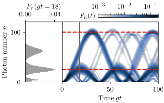
In typical situations, the photon number distribution consists of two oscillating packets, which are symmetric only if and therefore cannot be distinguished in this case. This qualitative picture imposed by the foregoing discussion is clearly supported by the numerical results presented in Sec. III. For , more than two packets are expected owing to the continuous split at the intermediate turning point. Similarly, this is confirmed by numerical calculations, as is shown in Fig. 3.
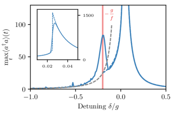
We now demonstrate that the analysis not only qualitatively, but also quantitatively reproduces the characteristics of the exact solution. To this end, we perform calculations with initial state , thereby isolating the packet in in the LDS-decoupled regime or the one in in the CDS-decoupled regime. In Fig. 4, we compare the maximum of the mean photon number with the turning points calculated in Sec. IV. With the expected exception at , both are in excellent agreement. As it turns out, the region around appears to be the point of transition between the CDS- and LDS-decoupled solutions.
V Influence of dissipative effects
In order to investigate, to what extend the previous results hold in realistic systems, which invariably experience some kind of dissipation, we turn our attention to solutions of the Liouville-von Neumann equation containing various dissipative contributions in Lindblad form, as detailed in Sec. II.
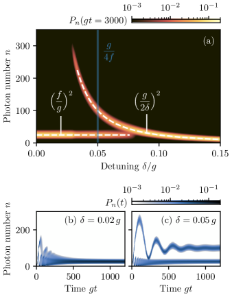
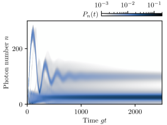
When isolating cavity losses, i.e. choosing , while , the oscillations of the packets are damped, resulting in an eventual stationary state. In general, the mean photon numbers of the individual packets in this stationary state differ from each other. This provides the possibility of bimodal distributions, the existence of which were already reported in Ref. [44]. However, only in the restricted set of parameters, given by
| (30) |
both packets are present in the stationary state. For values of the detuning only one packet with mean photon number
| (31) |
and for only one with mean photon number
| (32) |
are seen [cf. Fig. 5(a)]. This is reflected in the transient behavior, as one of the packets experiences considerable decay in the respective parameter regions. Illustrative examples of the dynamics in single- and dual-packet cases are shown in Figs. 5(b) and 5(c). It is to be noted, that the rules of thumb given in Eqs. (31) and (32) only hold for sufficiently low decay rates. Obviously, for increasing values of , there will be a transition to a stationary state with photons in the limit .
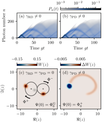
Examining now the decay channels of the TLS while neglecting cavity losses, we find little qualitative difference between the effects of radiative decay and pure dephasing. Examples of both cases are shown in Figs. 6(a) and 6(b) respectively. In contrast to the previously studied situation, the oscillations are not damped, but rather the packets themselves disperse until any discernible structure is lost. Further, a number of additional packets are noticeable, which even reach higher photon numbers than those without dissipation. Their origin can be understood in the LDS-decoupled case discussed in Sec. IV.1. With the help of the phase space operators
| (33a) | ||||
| (33b) | ||||
the effective Hamiltonian operators that describe the photonic evolution within the isolated branches are written as [cf. Eq. (9)]
| (34) |
From this expression, we can immediately read off that parts of the Wigner function corresponding to the TLS state will travel along ellipses around the center with its width in direction scaled by a factor of with respect to its width in direction. This is visualized in Fig. 6(c) using a numerical calculation without any dissipation. For the sake of clarity, we consider an initial state of for analyzing the influence of dephasing. In the absence of any dissipation, the Wigner function resembles a Gaussian shape following the trajectory
| (35) |
Pure dephasing induces transitions between the LDS while the photonic state remains unchanged. Hence, the original -solution is depleted leaving behind a trail of -states, where each part of this trail now orbits the center [cf. Fig. 6(d)]. By this mechanism, significantly higher photon numbers are reached. For instance, sections which are generated at times , i.e. when the original packet has reached its maximum [cf. Eq. (12)], will eventually reach corresponding to a photon number of . The appearance of additional packets is now attributed to situations in which large parts of the trail accumulate around similar photon numbers. This interpretation is consistent with the fact, that the additional packets are sharply visible only during short periods of time.
The effects of photonic and electronic dissipation combine in a straight-forward manner if both are taken into account concomitantly. An example of this is shown in Fig. 7. The packets induced by electronic dephasing as well as the main packets perform damped oscillations. It is to be noted, that the upper packet is of considerably lower probability compared to the case of mere cavity losses.
VI Conclusion
We have studied the Jaynes–Cummings model with strong cw driving of the TLS. We therein recovered the known result of a singular packet with oscillating mean photon number if the cavity is resonant to the external driving. If the driving is slightly detuned with respect to the frequency of the cavity, two or more packets simultaneously oscillate with considerably different characteristics.
When taking into account various forms of dissipation, the oscillatory patterns remain present transiently. Radiative decay and polarization dephasing of the TLS largely lead to the structure becoming indistinct whereas cavity losses damp the oscillations themselves. We found that the latter results in the decay of one of two packets depending on the value of the detuning. Only in a narrow transition region both packets remain stable under cavity losses, opening the possibility of bimodal stationary states.
We have presented a very simple way of preparing highly nonclassical photon states. We can expect to find these states in numerous physical systems, owing to the universality of the model. Our results might pave the way to photonic applications in particular new methods of quantum information processing that either exploit the bimodal stationary photon number distribution or the characteristic transient structures in the distribution to encode quantum information. It should be noted that modern measurement techniques allow for a direct experimental monitoring of the photon number distribution [45, 46, 47] and therefore for a readout of information stored in the distribution.
Appendix A Effective Hamiltonian in the strong driving limit
The Hamiltonian in the LDS basis reads
| (36) |
where and are the ladder operators defined by
| (37) |
and . As described in Sec. IV, the cross-coupling, mediated by the operator , only enacts a small effect on the dynamics at sufficiently low photon numbers. We therefore seek a unitary transformation
| (38) |
with , such that
| (39) |
is diagonal in the LDS-basis, thereby treating the influence of the cross-coupling perturbatively (for a detailed account of this method, see Ref. [48]). To second order in this is achieved by choosing
| (40) |
where
| (41a) | ||||
| (41b) | ||||
| (41c) | ||||
| (41d) | ||||
| (41e) | ||||
Using this expression we obtain up to an additive constant
| (42) |
where is given by Eq. (9).
Since is quadratic in the photonic annihilation and creation operators, it can be readily diagonalised
| (43) |
such that , fulfill bosonic commutation relations. We use the ansatz
| (44) |
with , according to which
| (45) |
By comparing coefficients with
| (46) |
and solving the resulting equations, we obtain the unique solution
| (47a) | ||||
| (47b) | ||||
| (47c) | ||||
After solving Eq. (44) for and , the mean photon number under evolution of with initial condition can be determined
| (48) |
Appendix B WKB analysis of a linear chain model
We consider the equation
| (49) |
which recovers Eq. (20) after identifying , and . In the limit , corresponding to slowly varying frequencies , we seek an asymptotic solution of the form
| (50) |
where and are smooth functions. In evaluating the expansion at neighboring excitation numbers, and are expanded in Taylor series
| (51) |
Inserting Eqs. (50) and (51) into Eq. (49) results to leading order in the eikonal equation
| (52) |
Since the right hand side of Eq. (52) is real, has to be either real, purely imaginary, or consist of a nonvanishing real part and a constant imaginary part of . These conform to the cases , and respectively. We thus conclude that exhibit wave-like behavior in the range given by
| (53) |
and exponential decay outside thereof.
In this work, we will not be interested in stating an explicit expression of or determining . The latter would be achieved by considering the higher order equations. For a detailed discussion of the present method, see Ref. [49] and references therein.
References
- Huang et al. [1983] G. M. Huang, T. J. Tarn, and J. W. Clark, On the controllability of quantum-mechanical systems, Journal of Mathematical Physics 24, 2608 (1983).
- Warren et al. [1993] W. S. Warren, H. Rabitz, and M. Dahleh, Coherent Control of Quantum Dynamics: The Dream Is Alive, Science 259, 1581 (1993).
- Rabitz et al. [2000] H. Rabitz, R. de Vivie-Riedle, M. Motzkus, and K. Kompa, Whither the Future of Controlling Quantum Phenomena?, Science 288, 824 (2000).
- Chu [2002] S. Chu, Cold atoms and quantum control, Nature 416, 206 (2002).
- Mabuchi and Khaneja [2005] H. Mabuchi and N. Khaneja, Principles and applications of control in quantum systems, International Journal of Robust and Nonlinear Control 15, 647 (2005).
- Greilich et al. [2006] A. Greilich, R. Oulton, E. A. Zhukov, I. A. Yugova, D. R. Yakovlev, M. Bayer, A. Shabaev, A. L. Efros, I. A. Merkulov, V. Stavarache, D. Reuter, and A. Wieck, Optical Control of Spin Coherence in Singly Charged Quantum Dots, Physical Review Letters 96, 227401 (2006).
- Rabitz [2009] H. Rabitz, Focus on Quantum Control, New Journal of Physics 11, 105030 (2009).
- Ramsay [2010] A. J. Ramsay, A review of the coherent optical control of the exciton and spin states of semiconductor quantum dots, Semiconductor Science and Technology 25, 103001 (2010).
- Sayrin et al. [2011] C. Sayrin, I. Dotsenko, X. Zhou, B. Peaudecerf, T. Rybarczyk, S. Gleyzes, P. Rouchon, M. Mirrahimi, H. Amini, M. Brune, J.-M. Raimond, and S. Haroche, Real-time quantum feedback prepares and stabilizes photon number states, Nature 477, 73 (2011).
- Jenkins and Ruostekoski [2012] S. D. Jenkins and J. Ruostekoski, Controlled manipulation of light by cooperative response of atoms in an optical lattice, Physical Review A 86, 031602 (2012).
- Krastanov et al. [2015] S. Krastanov, V. V. Albert, C. Shen, C.-L. Zou, R. W. Heeres, B. Vlastakis, R. J. Schoelkopf, and L. Jiang, Universal control of an oscillator with dispersive coupling to a qubit, Physical Review A 92, 040303 (2015).
- Ballantine and Ruostekoski [2021] K. E. Ballantine and J. Ruostekoski, Quantum Single-Photon Control, Storage, and Entanglement Generation with Planar Atomic Arrays, PRX Quantum 2, 040362 (2021).
- Ma et al. [2021] W.-L. Ma, S. Puri, R. J. Schoelkopf, M. H. Devoret, S. M. Girvin, and L. Jiang, Quantum control of bosonic modes with superconducting circuits, Science Bulletin 66, 1789 (2021).
- Cosacchi et al. [2022a] M. Cosacchi, T. Seidelmann, A. Mielnik-Pyszczorski, M. Neumann, T. K. Bracht, M. Cygorek, A. Vagov, D. E. Reiter, and V. M. Axt, Deterministic Photon Storage and Readout in a Semimagnetic Quantum Dot–Cavity System Doped with a Single Mn Ion, Advanced Quantum Technologies 5, 2100131 (2022a).
- Michler et al. [2000] P. Michler, A. Kiraz, C. Becher, W. V. Schoenfeld, P. M. Petroff, L. Zhang, E. Hu, and A. Imamoğlu, A Quantum Dot Single-Photon Turnstile Device, Science 290, 2282 (2000).
- Varcoe et al. [2000] B. T. H. Varcoe, S. Brattke, M. Weidinger, and H. Walther, Preparing pure photon number states of the radiation field, Nature 403, 743 (2000).
- Hofheinz et al. [2008] M. Hofheinz, E. M. Weig, M. Ansmann, R. C. Bialczak, E. Lucero, M. Neeley, A. D. O’Connell, H. Wang, J. M. Martinis, and A. N. Cleland, Generation of Fock states in a superconducting quantum circuit, Nature 454, 310 (2008).
- Zhou et al. [2012] X. Zhou, I. Dotsenko, B. Peaudecerf, T. Rybarczyk, C. Sayrin, S. Gleyzes, J. M. Raimond, M. Brune, and S. Haroche, Field Locked to a Fock State by Quantum Feedback with Single Photon Corrections, Physical Review Letters 108, 243602 (2012).
- Somaschi et al. [2016] N. Somaschi, V. Giesz, L. De Santis, J. C. Loredo, M. P. Almeida, G. Hornecker, S. L. Portalupi, T. Grange, C. Antón, J. Demory, C. Gómez, I. Sagnes, N. D. Lanzillotti-Kimura, A. Lemaítre, A. Auffeves, A. G. White, L. Lanco, and P. Senellart, Near-optimal single-photon sources in the solid state, Nature Photonics 10, 340 (2016).
- Schweickert et al. [2018] L. Schweickert, K. D. Jöns, K. D. Zeuner, S. F. Covre da Silva, H. Huang, T. Lettner, M. Reindl, J. Zichi, R. Trotta, A. Rastelli, and V. Zwiller, On-demand generation of background-free single photons from a solid-state source, Applied Physics Letters 112, 093106 (2018).
- Cosacchi et al. [2020a] M. Cosacchi, J. Wiercinski, T. Seidelmann, M. Cygorek, A. Vagov, D. E. Reiter, and V. M. Axt, On-demand generation of higher-order Fock states in quantum-dot–cavity systems, Physical Review Research 2, 033489 (2020a).
- Eleuch et al. [1999] H. Eleuch, J. M. Courty, G. Messin, C. Fabre, and E. Giacobino, Cavity QED effects in semiconductor microcavities, Journal of Optics B: Quantum and Semiclassical Optics 1, 1 (1999).
- Lutterbach and Davidovich [2000] L. G. Lutterbach and L. Davidovich, Production and detection of highly squeezed states in cavity QED, Physical Review A 61, 023813 (2000).
- Garcés and de Valcárcel [2016] R. Garcés and G. J. de Valcárcel, Strong vacuum squeezing from bichromatically driven Kerrlike cavities: from optomechanics to superconducting circuits, Scientific Reports 6, 21964 (2016).
- Joshi et al. [2017] C. Joshi, E. K. Irish, and T. P. Spiller, Qubit-flip-induced cavity mode squeezing in the strong dispersive regime of the quantum Rabi model, Scientific Reports 7, 45587 (2017).
- Jabri and Eleuch [2022] H. Jabri and H. Eleuch, Squeezed vacuum interaction with an optomechanical cavity containing a quantum well, Scientific Reports 12, 3658 (2022).
- Brune et al. [1996] M. Brune, E. Hagley, J. Dreyer, X. Maître, A. Maali, C. Wunderlich, J. M. Raimond, and S. Haroche, Observing the Progressive Decoherence of the “Meter” in a Quantum Measurement, Physical Review Letters 77, 4887 (1996).
- van Enk and Hirota [2001] S. J. van Enk and O. Hirota, Entangled coherent states: Teleportation and decoherence, Physical Review A 64, 022313 (2001).
- Mirrahimi et al. [2014] M. Mirrahimi, Z. Leghtas, V. V. Albert, S. Touzard, R. J. Schoelkopf, L. Jiang, and M. H. Devoret, Dynamically protected cat-qubits: a new paradigm for universal quantum computation, New Journal of Physics 16, 045014 (2014).
- Ofek et al. [2016] N. Ofek, A. Petrenko, R. Heeres, P. Reinhold, Z. Leghtas, B. Vlastakis, Y. Liu, L. Frunzio, S. M. Girvin, L. Jiang, M. Mirrahimi, M. H. Devoret, and R. J. Schoelkopf, Extending the lifetime of a quantum bit with error correction in superconducting circuits, Nature 536, 441 (2016).
- Cosacchi et al. [2021] M. Cosacchi, T. Seidelmann, J. Wiercinski, M. Cygorek, A. Vagov, D. E. Reiter, and V. M. Axt, Schr\"odinger cat states in quantum-dot-cavity systems, Physical Review Research 3, 023088 (2021).
- Ralph et al. [2003] T. C. Ralph, A. Gilchrist, G. J. Milburn, W. J. Munro, and S. Glancy, Quantum computation with optical coherent states, Physical Review A 68, 042319 (2003).
- Zoller et al. [2005] P. Zoller, T. Beth, D. Binosi, R. Blatt, H. Briegel, D. Bruss, T. Calarco, J. I. Cirac, D. Deutsch, J. Eisert, A. Ekert, C. Fabre, N. Gisin, P. Grangiere, M. Grassl, S. Haroche, A. Imamoglu, A. Karlson, J. Kempe, L. Kouwenhoven, S. Kröll, G. Leuchs, M. Lewenstein, D. Loss, N. Lütkenhaus, S. Massar, J. E. Mooij, M. B. Plenio, E. Polzik, S. Popescu, G. Rempe, A. Sergienko, D. Suter, J. Twamley, G. Wendin, R. Werner, A. Winter, J. Wrachtrup, and A. Zeilinger, Quantum information processing and communication, The European Physical Journal D - Atomic, Molecular, Optical and Plasma Physics 36, 203 (2005).
- Lo et al. [2014] H.-K. Lo, M. Curty, and K. Tamaki, Secure quantum key distribution, Nature Photonics 8, 595 (2014).
- Acín et al. [2018] A. Acín, I. Bloch, H. Buhrman, T. Calarco, C. Eichler, J. Eisert, D. Esteve, N. Gisin, S. J. Glaser, F. Jelezko, S. Kuhr, M. Lewenstein, M. F. Riedel, P. O. Schmidt, R. Thew, A. Wallraff, I. Walmsley, and F. K. Wilhelm, The quantum technologies roadmap: a European community view, New Journal of Physics 20, 080201 (2018).
- Cosacchi et al. [2020b] M. Cosacchi, T. Seidelmann, F. Ungar, M. Cygorek, A. Vagov, and V. M. Axt, Transiently changing shape of the photon number distribution in a quantum-dot–cavity system driven by chirped laser pulses, Physical Review B 101, 205304 (2020b).
- Schimpf et al. [2021] C. Schimpf, M. Reindl, D. Huber, B. Lehner, S. F. Covre Da Silva, S. Manna, M. Vyvlecka, P. Walther, and A. Rastelli, Quantum cryptography with highly entangled photons from semiconductor quantum dots, Science Advances 7, eabe8905 (2021).
- Vajner et al. [2022] D. A. Vajner, L. Rickert, T. Gao, K. Kaymazlar, and T. Heindel, Quantum Communication Using Semiconductor Quantum Dots, Advanced Quantum Technologies 5, 2100116 (2022).
- Gao et al. [2022] T. Gao, L. Rickert, F. Urban, J. Große, N. Srocka, S. Rodt, A. Musiał, K. Żołnacz, P. Mergo, K. Dybka, W. Urbańczyk, G. Sȩk, S. Burger, S. Reitzenstein, and T. Heindel, A quantum key distribution testbed using a plug&play telecom-wavelength single-photon source, Applied Physics Reviews 9, 011412 (2022).
- Bozzio et al. [2022] M. Bozzio, M. Vyvlecka, M. Cosacchi, C. Nawrath, T. Seidelmann, J. C. Loredo, S. L. Portalupi, V. M. Axt, P. Michler, and P. Walther, Enhancing quantum cryptography with quantum dot single-photon sources, npj Quantum Information 8, 1 (2022).
- Cosacchi et al. [2022b] M. Cosacchi, A. Mielnik-Pyszczorski, T. Seidelmann, M. Cygorek, A. Vagov, D. E. Reiter, and V. M. Axt, -photon bundle statistics on different solid-state platforms, Physical Review B 106, 115304 (2022b).
- Chough and Carmichael [1996] Y. T. Chough and H. J. Carmichael, Nonlinear oscillator behavior in the Jaynes-Cummings model, Physical Review A 54, 1709 (1996).
- Barnett and Radmore [2002] S. M. Barnett and P. M. Radmore, Methods in Theoretical Quantum Optics (Oxford University Press, 2002) pp. 114–125.
- Cygorek et al. [2017] M. Cygorek, A. M. Barth, F. Ungar, A. Vagov, and V. M. Axt, Nonlinear cavity feeding and unconventional photon statistics in solid-state cavity QED revealed by many-level real-time path-integral calculations, Physical Review B 96, 201201 (2017).
- Schlottmann et al. [2018] E. Schlottmann, M. von Helversen, H. A. Leymann, T. Lettau, F. Krüger, M. Schmidt, C. Schneider, M. Kamp, S. Höfling, J. Beyer, J. Wiersig, and S. Reitzenstein, Exploring the Photon-Number Distribution of Bimodal Microlasers with a Transition Edge Sensor, Physical Review Applied 9, 064030 (2018).
- Schmidt et al. [2018] M. Schmidt, M. von Helversen, M. López, F. Gericke, E. Schlottmann, T. Heindel, S. Kück, S. Reitzenstein, and J. Beyer, Photon-Number-Resolving Transition-Edge Sensors for the Metrology of Quantum Light Sources, Journal of Low Temperature Physics 193, 1243 (2018).
- Helversen et al. [2019] M. v. Helversen, J. Böhm, M. Schmidt, M. Gschrey, J.-H. Schulze, A. Strittmatter, S. Rodt, J. Beyer, T. Heindel, and S. Reitzenstein, Quantum metrology of solid-state single-photon sources using photon-number-resolving detectors, New Journal of Physics 21, 035007 (2019).
- Cohen-Tannoudji et al. [2004] C. Cohen-Tannoudji, J. Dupont-Roc, and G. Grynberg, Atom-Photon Interactions: Basic Processes and applications (Wiley-VCH, 2004) pp. 38–46.
- Holmes [2013] M. H. Holmes, Introduction to perturbation methods, 2nd ed. (Springer, New York, NY, 2013) pp. 286–288.