Excitations of a binary supersolid

Abstract

We predict a rich excitation spectrum of a binary dipolar supersolid in a linear crystal geometry, where the ground state consists of two partially immiscible components with alternating, interlocking domains. We identify three Goldstone branches, each with first-sound, second-sound or spin-sound character. In analogy with a diatomic crystal, the resulting lattice has a two-domain primitive basis and we find that the crystal (first-sound-like) branch is split into optical and acoustic phonons. We also find a spin-Higgs branch that is associated with the supersolid modulation amplitude.

The engineering of crystal phonons—or quantized sound waves—is an important challenge for ultracold gases [1, 2], not least as simulators of solids with their central role in governing a material’s thermodynamic and electrical properties [3, 4]. Phonons had long eluded periodic optical potentials with neutral atoms, owing to the infinite lattice stiffness. Major milestones have now been reached with the realization of supersolids, inherently possessing both the dissipationless flow of superfluids and the elastic crystalline structure of solids. Despite their prediction over 50 years ago [5, 6, 7, 8], supersolids were realized only recently using ultracold gases with dipolar interactions [9, 10, 11, 12] and spin-orbit coupling [13, 14]. Supersolid phonons are of interest for a range of systems [15, 16, 17, 18, 19, 20, 21, 22], and experiments have begun probing them in dipolar condensates [23, 24, 25, 26, 27, 28].

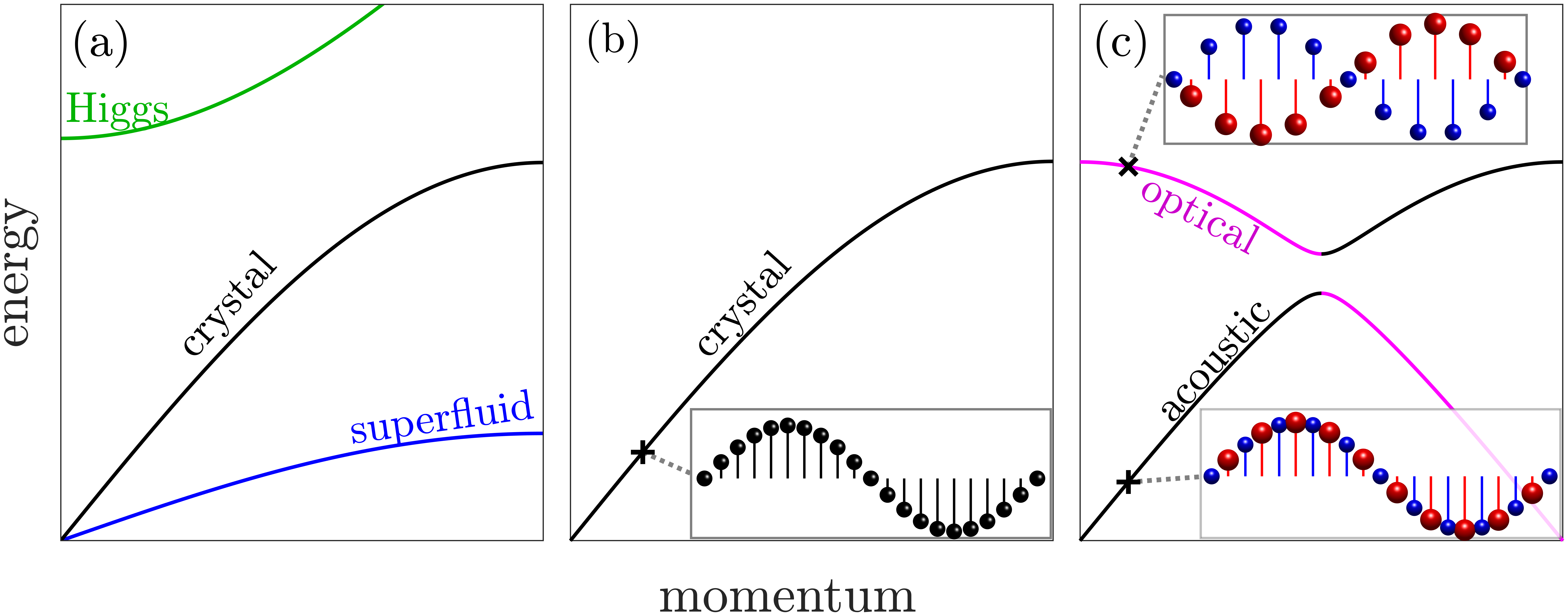
Figure 1: Schematic excitations for linear (a) single-component dipolar supersolid, and ordinary (b) monatomic and (c) diatomic crystals, with optical and acoustic phonons.

For linear supersolids, a crystal phonon branch [Fig. 1(a)] appears similar to a regular solid [Fig. 1(b)], emerging from a spontaneously broken continuous translational symmetry . A second Goldstone branch of superfluid phonons arises from breaking a global $U(1)$ gauge symmetry associated with the condensate order parameter [30]. Higgs modes [24, 25, 31] connected with a roton instability of the unmodulated phase [32, 33, 34, 35, 36, 37] are also present. There has been a significant undertaking to develop a general hydrodynamic model of supersolidity, e.g., see [38, 39, 40], with compelling new advances [41, 42]. The periodic modulation of the density reduces the superfluid fraction [7] and—in analogy with finite-temperature superfluids—the lower phonon branch has a second-sound character, while the upper branch consists of first-sound-like modes [41, 42]. In dipolar supersolids, an intimate connection between the second-sound velocity and the superfluid fraction has been proposed as a practical means to measuring superfluidity [42].

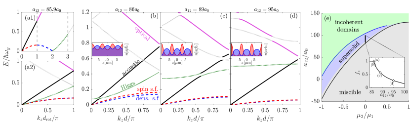
Figure 2: Binary supersolid dispersion. (a1) Excitation energies versus momentum for a uniform miscible state close to the transition. Sections of the spin (lower) and density (upper) branches have been color-coded, and these are folded into the first BZ in (a2) to demonstrate the origins of the supersolid branches that emerge in the next panels. (b)-(d) Supersolid excitations for increasing $a_{12}$, with insets showing integrated linear densities. (e) Phase diagram. Solid colors correspond to phases calculated using the variational method. For comparison, full 3D calculations are shown as solid lines, closely matching the corresponding uniform-supersolid (black) and supersolid-incoherent domain (blue) boundaries. Inset: superfluid fraction for a path across the transition (black vertical line) with the corresponding points for panels (a)-(d) indicated.

Recent theory predicts the existence of binary dipolar supersolids, where two superfluids combine to form a periodically modulated state [43, 44, 45, 46, 47, 48]. For a dipole imbalance between components, a special class forms partially immiscible alternating domains, with the ground state stabilized by an interplay between the dipolar and contact interactions [45, 46, 48]. Experimental advances with magnetic atoms suggest that binary supersolids may soon be realizable [49, 50, 51, 43, 52], yet theoretical knowledge of the excitation spectrum is absent. The two global gauge symmetries can spontaneously break independently, but intercomponent interactions mean that only a single translational symmetry (per spatial dimension) can spontaneously break, while the other is broken explicitly [15]. Hence, for an $\mathcal{N}$-component supersolid in $D$ dimensions, one might expect $D+\mathcal{N}$ Goldstone modes. The lattice of binary supersolids can be described by a multidomain primitive basis, and further understanding may be gleaned by analogy with nonsuperfluid crystals. In ordinary crystal lattices with two atoms per primitive cell, the phonon branch of a monotonic linear crystal [Fig. 1(b)] is replaced by a gapped spectrum in a diatomic lattice [Fig. 1(c)] [53, 4]. The size of the Brillouin zone (BZ) is thus halved and folded (magenta curves), with the lower acoustic (upper optical) branch being characterized by in-phase (out-of-phase) motions between nearest neighbors [see insets].

In this Letter, we reveal the emergence and evolution of the excitation spectra of binary dipolar supersolids in an infinite tube. From the uniform miscible phase, the spin branch—related to fluctuations driving phase separation—develops rotonic excitations, and their instability is connected with the formation of the supersolid, having partially immiscible, alternating domains. A rich excitation spectrum emerges with three Goldstone modes, where in addition to a second-sound-like branch there is a spin-sound branch, and the first-sound-like branch divides into optical and acoustic phonons. The modulation amplitude of the supersolid is associated with a spin-Higgs branch.

We consider a pair of distinguishable BECs with wavefunctions $\Psi_{i}$ ($i=1,2$), described by two coupled Gross-Pitaevskii equations (GPEs) [54]. The atoms are trapped in an infinite tube potential oriented along the $z$ axis, $V_{i}(\textbf{r})=\frac{1}{2}m_{i}(\omega_{x}^{2}x^{2}+\omega_{y}^{2}y^{2})$. To remain firmly in the linear crystal regime we select trapping frequencies $\{\omega_{x},\omega_{y}\}/2\pi=\{300,100\}$ Hz. To highlight the novel features of a dipole-imbalanced mixture, we take balanced intraspecies scattering lengths $a_{ii}=130a_{0}$, average linear densities $\bar{n}_{i}=200\mu\mathrm{m}^{-1}$ and the mass of ${}^{164}\mathrm{Dy}$, $m_{i}=164\mathrm{u}$. For the dipoles, which are polarized along $y$, we take $\mu_{1}=9.93\mu_{\mathrm{B}}$ and unless otherwise stated, we consider the second component as nondipolar $\mu_{2}=0$. We generalize a 3D variational theory developed in Ref. [55] to two components. Decomposing the wavefunctions as $\Psi_{i}(\textbf{r})=\psi_{i}(z)\phi_{i}(x,y)$, we then assume radial degrees of freedom are described by $\phi_{i}(x,y)=\frac{1}{\ell_{i}\sqrt{\pi}}\exp\left[-(\eta_{i}x^{2}+y^{2}/\eta_{i})/(2\ell_{i}^{2})\right]$, where $\eta_{i}$ and $\ell_{i}$ are variational parameters that are determined by minimizing the energy. The ground state is calculated by solving the two-component GPEs in imaginary time. By making use of Fourier copies along $z$, only a single primitive unit cell needs to be simulated to reach the ground state in the thermodynamic limit, while the crystal lattice spacing $d$ is varied until the energy is minimized. The excitation spectrum is calculated using a Bogoliubov-de Gennes (BdG) formalism [54].

Longitudinal excitation spectra within the first BZ are shown in Fig. 2 for various interspecies coupling constants $a_{12}$, ranging from near the supersolid transition point [Fig. 2 (a)]—where the density is still uniform—to deep inside the supersolid regime [Fig. 2 (d)]. Mode types are labeled in panel (b), showing a Goldstone acoustic phonon branch and two Goldstone superfluid (s.f.) branches, where the latter will later be distinguished as being either spin or density dominated. Spin Higgs and optical branches are also labeled, while higher superfluid modes that are not the central focus of this work are plotted as gray dotted lines. As $a_{12}$ is increased, the reduction of intersite superfluid is apparent in the linear density plots (insets), where the dipolar (nondipolar) component is shown in red (blue). The increasingly isolated domains act to flatten the bands of the superfluid modes [dotted/dashed lines in Fig. 2 (d)], leaving the nontrivial optical and acoustic crystal branches to closely resemble a solid without superfluidity [Fig. 1 (c)].

To understand the origin of each branch, Fig. 2 (a1) shows the excitation spectrum in the unmodulated miscible phase very close to the transition. The density branch remains hard, while the spin branch has developed a roton minimum that softens (lowers) and becomes unstable as the transition is crossed. Defining a fictitious BZ boundary for a lattice vector corresponding to the roton wavelength, $d_{\mathrm{rot}}$, we then color parts of both branches as they cross through each BZ, with the BZ ‘edges’ shown as vertical dashed lines. Figure 2 (a2) shows the same data, but with the spectrum folded into the reduced zone scheme. From this mapping, it becomes clear that crystal modes emerge from the density branch, with the lower (upper) part becoming the acoustic (optical) branch. In contrast, superfluid modes emerge from the spin branch, with the spin Higgs mode connecting with the unstable spin rotons at the transition.

Situating our system within the context of a larger available parameter space, we show in Fig. 2 (e) a phase diagram for a range of dipolar mixtures (fixed $\mu_{1}=9.93\mu_{\rm B}$ but varying $\mu_{2}$). We classify phases using the upper bound on the superfluid fraction as outlined by Leggett, $f_{s}^{(i)}=\frac{d^{2}}{N_{i}}\left[\int_{\mathrm{uc}}\mathrm{d}z\left(\int\mathrm{d}x\mathrm{d}y|\Psi_{i}|^{2}\right)^{-1}\right]^{-1}$, where $N_{i}=\bar{n}_{i}d=\int_{\mathrm{uc}}\mathrm{d}z|\psi_{i}|^{2}$ is the particle number of component $i$ within a unit cell (uc), such that the reduction in total moment of inertia of the composite system is related to the total superfluid fraction, $f_{s}=(N_{1}f_{s}^{(1)}+N_{2}f_{s}^{(2)})/(N_{1}+N_{2})$. In the miscible phase (gray), there is no density modulation in the region immediately below the supersolid phase and $f_{s}=1$ . Increasing $a_{12}$ leads to a transition to the supersolid ($0.1<f_{s}<1$) phase and subsequently to the incoherent domain ($f_{s}\leq 0.1$) regime. The supersolid phase can be seen to extend over a broad range of dipole combinations, and we have checked (not shown) that our excitation findings are qualitatively representative throughout this region. We also perform full 3D ground state calculations (solid curves) to corroborate our predictions for the uniform-to-supersolid and supersolid-to-incoherent domain phase boundaries, and find good agreement throughout the phase diagram. The inset shows how $f_{s}$ changes as the transition is crossed for the dipolar-nondipolar system, with the locations of the preceding panels of Fig. 2 also indicated.

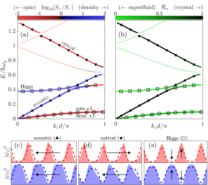
Figure 3: Branch identification for dipolar-nondipolar mixture with $a_{12}=90a_{0}$. (a) Excitation branches are shown and colored based on the relative strength of the dynamic structure factor. Symbols to guide the eye indicate acoustic ($\blacktriangle$) and optical ($\blacktriangledown$) crystal branches, a spin Higgs ($\square$) branch, as well as spin- ($\ocircle$) and density- ($\odot$) superfluid branches. (b) Superfluid versus crystal character (see main text). (c)-(e) Examples of long-wavelength modes, where one can see the ground state (dashed) and the same state with the corresponding BdG excitation added (shaded) – see also videos [54].

The lower panels of Fig. 3 correspond to exemplary BdG modes of the binary supersolid system. The ground state over a few lattice sites is shown with dashed lines, and the same states including the corresponding excitations are shown with shading. The BdG modes are included with a sufficiently large amplitude to emphasize the motion. The acoustic and optical modes are dominated by spatial oscillations of the domains, in-phase and out-of-phase, respectively, while for the spin Higgs mode, the domains remain stationary but the spin-density amplitude ($||\psi_{2}|^{2}-|\psi_{1}|^{2}|$) changes.

For a quantitative understanding of the excitation spectrum, we consider two measures of branch identification. In Fig. 3 (a) we plot the contribution from each excitation $\kappa$ to the dynamic structure factor [57, 58],

$$S_{\pm}(k_{z},\omega)=\sum_{\kappa}\left|\delta\tilde{n}^{\pm}_{\kappa}(k_{z})\right|^{2}\delta(\omega-\omega_{\kappa})\,,$$ (1)

where $\delta\tilde{n}^{\pm}_{\kappa}(k_{z})=\int_{0}^{L}\mathrm{d}z\;\mathrm{e}^{-\mathrm{i}k_{z}z}[\delta n_{\kappa,1}(z)\pm\delta n_{\kappa,2}(z)]$, the excitation energies are $\omega_{\kappa}=E_{\kappa}/\hbar$ and the density fluctuations are $\delta n_{\kappa,i}(z)=\psi_{i}(z)[u_{\kappa,i}(z)-v_{\kappa,i}(z)]$, with the modes $u_{\kappa,i}$ and $v_{\kappa,i}$ being the BdG amplitudes [54]. In determining branch character, we simulate a larger system of size $L=N_{\mathrm{uc}}d$ for $N_{\mathrm{uc}}=96$. The spectrum is colored by the relative strength of the spin or density dynamic structure factor along each branch, with blue representing a stronger signal in $S_{+}$, and red for $S_{-}$. The density $(+)$ structure factor dominates when the components oscillate in-phase, while the spin $(-)$ structure factor is stronger for out-of-phase fluctuations.

In Fig. 3 (b) we plot quantity $\bar{\mathcal{R}}_{\kappa}$ as a measure of the crystal versus superfluid character of each quasi-particle excitation labeled by quantum number $\kappa$. This is calculated by comparing the average motion caused by the excitation around the density peaks of each component relative to the interstitial regions, and is therefore sensitive to its crystal ($\mathcal{\bar{R}}_{\kappa}\gtrsim 1$) or superfluid ($\mathcal{\bar{R}}_{\kappa}\ll 1$) character. See Supplemental Material [54] for further details, or Ref. [25] for a related calculation for a single-component system.

Both measures in Fig. 3 demonstrate that as energy bands approach one another, avoided crossings occur and coupling between branches results in hybridization of mode character in these regions. Nevertheless, both the optical and acoustic branches can clearly be identified by their strong crystal character [black curves in Fig. 3 (b)], and they can be distinguished from one another by the relative strength of the density or spin structure factors [Fig. 3 (a)]. The strong density character of the acoustic branch implies that the crystal excitations of both components occur in the same direction, i.e., neighboring domains move in phase [Fig. 3 (c)], while for the optical branch (spin dominated) the components oppose one another [Fig. 3 (d)].

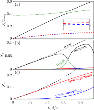
Figure 4: Goldstone mode contributions to the static structure factor for a dipolar-nondipolar mixture at $a_{12}=90a_{0}$. (a) Low energy spectrum showing spin Higgs and three Goldstone branches. (b) Density and (c) spin static structure factors shown as black-dashed lines, with the contributions from each branch (solid) color-coded for easy comparison with (a).

The two-component nature of our system (i.e. two domains per unit cell) affords greater flexibility in addressing spin and density excitations. Most notably, if an excitation predominantly couples to the spin structure factor for momentum transfer in the first BZ, in the second BZ it will predominantly couple to the density structure factor. For example, the spin Higgs excitations modulate the relative immiscibility of the supersolid state, and Fig. 3 (a) shows a strong signal in $S_{+}$ within the first BZ—since the modulation amplitudes of neighboring domains oscillate in phase [Fig. 3 (e)]—but these same modes are dominated by $S_{-}$ in the second BZ (not shown), where this immiscibility occurs at the roton wavelength. The situation is reversed for the optical branch, which emerges from the density branch in the unmodulated regime (Fig. 2), but has strong spin character in the first BZ [Fig. 3 (a)]. An interesting feature of our system, and in contrast to an idealized solid with point-like particles, is that modes of higher energy can probe the internal structure of individual lattice sites.

To differentiate the characteristics of the three Goldstone branches, we turn to the density and spin static structure factors defined as $S_{\pm}(k_{z})\equiv\int\mathrm{d}\omega\;S_{\pm}(k_{z},\omega)/N$, respectively, with total particle number $N=N_{\mathrm{uc}}(N_{1}+N_{2})$. Figure 4 (b) shows the total density structure factor (dashed line), along with the contributions from each the three Goldstone branches, and the Higgs branch, colored to match the respective energy branches in Fig. 4 (a). While the density ($+$) static structure factor is dominated by the acoustic branch (black solid line) at low and high momenta, there is significant mixing close to the avoided crossing between the Higgs and acoustic branches. In the spin ($-$) static structure factor [Fig. 4 (c)], there is a strong distinction in the contributions from the two superfluid Goldstone branches, allowing us to distinguish the “spin” superfluid branch from the “density” superfluid branch. Further, we have checked that the density (spin) branches create superfluid flows in the two components that align with (oppose) one another [54]. Closer to the phase transition (not shown), the distinction becomes less clear and both low superfluid branches contribute with comparable weight to the structure factor.

In summary, we have performed the first study of the excitation spectrum of a binary dipolar supersolid, focussing on an elongated geometry. Three Goldstone branches emerge due to the spontaneous breaking of one translational symmetry and two gauge symmetries, confirming the anticipated $D+\mathcal{N}$ Goldstone modes of multicomponent supersolids. In addition to Goldstone modes with first- and second-sound character, we identify a Goldstone branch with spin-sound character. Further, in analogy with ordinary solids, the spectrum exhibits both optical and acoustic phonon branches, and in addition, a spin Higgs branch emerging from the spin roton.

We expect our findings to be attainable with current experimental capabilities, thanks to their generality across a wide parameter space of imbalanced mixtures, including heteronuclear combinations of magnetic atoms [49, 50, 51, 43, 52] and homonuclear mixtures with various spin projections [59]. Since immiscible binary supersolids do not require quantum fluctuations for their stabilization, in contrast to other dipolar supersolids, we expect lower densities and crystals with significantly more lattice sites. Ideal geometries include strongly prolate trapping or toroidal traps [60, 61, 62, 63, 42, 64, 65]. Our work also opens intriguing perspectives for future work to develop a general hydrodynamic model and an effective Lagrangian for $\mathcal{N}$-component supersolids [38, 39, 40, 41, 42].

Acknowledgements:— R. B., T. B., F. F. and W. K. acknowledge financial support by the ESQ Discovery programme (Erwin Schrödinger Center for Quantum Science & Technology), hosted by the Austrian Academy of Sciences (ÖAW). D. B., P. B. B. and A. C. L.  acknowledge support from the Marsden Fund of the Royal Society of New Zealand. R. B. also acknowledges the Austrian Science Fund (FWF): P 36850-N. F. F. acknowledges support from the European Research Council through the Advanced Grant DyMETEr (No. 101054500), the DFG/FWF via Dipolare E2 (No. I4317-N36) and, with T. B., a joint project grant from the FWF (No. I4426).

I Supplementary Materials

I.1 GPE and Variational theory

The two-component dipolar GPE is given by,

$$\mathrm{i}\hbar\frac{\partial\Psi_{i}(\textbf{r})}{\partial t}= \Biggl{[}-\frac{\hbar^{2}\nabla^{2}}{2m_{i}}+V_{i}(\textbf{r})+\sum_{j}g_{ij}n_{j}(\textbf{r})$$

$$+\sum_{j}\int\mathrm{d}\textbf{r}^{\prime}U_{ij}(\textbf{r}-\textbf{r}^{\prime})n_{j}(\textbf{r}^{\prime})\Biggr{]}\Psi_{i}(\textbf{r})\;,$$ (S1)

with atomic mass $m_{i}$, density $n_{i}(\textbf{r})=|\Psi_{i}(\textbf{r})|^{2}$, contact interaction strength $g_{ij}=2\pi\hbar^{2}a_{ij}(m_{i}+m_{j})/(m_{i}m_{j})$, and trapping potential $V_{i}(\textbf{r})=\frac{1}{2}m_{i}(\omega_{x}^{2}x^{2}+\omega_{y}^{2}y^{2})$. The dipole-dipole interaction (DDI) between particles of magnetic moment $\mu_{i}$ and $\mu_{j}$ is given by $U_{ij}(\textbf{r})=\mu_{0}\mu_{i}\mu_{j}(1-3\cos^{2}\theta)/4\pi|\textbf{r}|^{3}$, where $\theta$ is the angle between the vector r joining two dipoles and the polarization direction, which we take to be the $y$ axis, and $\mu_{0}$ is the vacuum permeability.

As described in the main text, we consider a reduced 3D variational theory by assuming the wavefunction takes the form, $\Psi_{i}(\textbf{r})=\psi_{i}(z)\varphi_{i}(x,y)$, with $\varphi_{i}(x,y)=\frac{1}{\ell_{i}\sqrt{\pi}}\exp\left[-(\eta_{i}x^{2}+y^{2}/\eta_{i})/(2\ell_{i}^{2})\right]$. We then multiply the GPE by $\varphi_{i}(x,y)$ and integrate over the azimuthal directions.

The integrated quasi-1D GPE is

$$\mathrm{i}\hbar\frac{\partial\psi_{i}(z,t)}{\partial t}= \;\Biggl{[}-\frac{\hbar^{2}}{2m_{i}}\frac{\partial^{2}}{\partial z^{2}}+\mathcal{E}_{\perp}^{i}+\sum_{j}\frac{g_{ij}}{2\pi\ell_{ij}^{2}}|\psi_{j}(z,t)|^{2}$$

$$+\sum_{j}\int\mathrm{d}z^{\prime}U_{ij}^{1\mathrm{D}}(z-z^{\prime})|\psi_{j}(z^{\prime},t)|^{2}\Biggr{]}\psi_{i}(z,t),$$ (S2)

where we have defined inter-component effective variational widths such that

$$4\ell_{ij}^{4}= \;(\ell_{i}^{2}\eta_{i}+\ell_{j}^{2}\eta_{j})(\ell_{i}^{2}/\eta_{i}+\ell_{j}^{2}/\eta_{j})$$ (S3)

$$\eta_{ij}^{2}= \;\frac{\ell_{i}^{2}\eta_{i}+\ell_{j}^{2}\eta_{j}}{\ell_{i}^{2}/\eta_{i}+\ell_{j}^{2}/\eta_{j}}~{},$$ (S4)

from which it follows naturally that $\ell_{ii}=\ell_{i}$ and $\eta_{ii}=\eta_{i}$. The energy per particle in component $i$ due to the trapping potential is given by

$$\mathcal{E}_{\perp}^{i}=\frac{\hbar^{2}}{4m_{i}\ell_{i}^{2}}\left(\eta_{i}+\frac{1}{\eta_{i}}\right)+\frac{1}{4}m_{i}\ell_{i}^{2}\left(\frac{\omega_{x}^{2}}{\eta_{i}}+\eta_{i}\omega_{y}^{2}\right)\;.$$ (S5)

For the integrated quasi-1D DDI, we make use of the expression developed in Ref.  [66] generalized to multiple variational widths

$$\mathcal{F}[U_{ij}^{1\text{D}}(z)]= \;\frac{\mu_{0}\mu_{i}\mu_{j}}{6\pi\ell_{ij}^{2}}\biggl{[}\frac{2-\eta_{ij}-3\cos^{2}\alpha}{1+\eta_{ij}}$$

$$+A_{\alpha}Q_{ij}^{2}\mathrm{e}^{Q_{ij}^{2}}\mathrm{Ei}\left(-Q_{ij}^{2}\right)\biggr{]}~{},$$ (S6)

where $\mathcal{F}$ denotes the Fourier transform, $\mathrm{Ei}(x)$ is the exponential integral, $A_{\alpha}=3\left(\frac{1-\cos^{2}\alpha}{1+\eta_{ij}}-\cos^{2}\alpha\right)$, $Q_{ij}(\alpha=\pi/2)=\frac{1}{\sqrt{2}}\eta_{ij}^{\frac{1}{4}}k\ell_{ij}$, and $Q_{ij}(\alpha=0)=\frac{1}{\sqrt{2}}\left(\frac{2\eta_{ij}}{1+\eta_{ij}^{2}}\right)^{\frac{2}{5}}k\ell_{ij}$ for dipole polarization angle $\alpha$.

I.2 BdG equations

Starting from the integrated quasi-1D GPE, we consider pertubations to the real ground state $\psi_{i}$ of the form

$$\tilde{\psi}_{i}(z,t)=\left\{\psi_{i}(z)+\lambda\left[u_{i}(z)\mathrm{e}^{-\mathrm{i}\omega t}-v_{i}^{*}(z)\mathrm{e}^{\mathrm{i}\omega^{*}t}\right]\right\}\mathrm{e}^{-\mathrm{i}\mu_{i}t/\hbar},$$ (S7)

where $\lambda$ is some small real perturbative parameter. Defining the linear operators $L_{i}$ and $X_{ij}[\;\cdot\;]$, acting on a function $w$,

$$L_{i}w_{i}\equiv \;-\frac{\hbar^{2}}{2m_{i}}\frac{\partial^{2}}{\partial z^{2}}w_{i}(z)+\mathcal{E}_{\perp}^{i}w_{i}(z)$$

$$+\sum_{j}\int\mathrm{d}z^{\prime}\;W_{ij}(z-z^{\prime})|\psi_{j}(z^{\prime})|^{2}w_{i}(z)$$ (S8)

$$X_{ij}[w_{j}]= \;\psi_{i}(z)\int\mathrm{d}z^{\prime}\;\psi_{j}(z^{\prime})W_{ij}(z-z^{\prime})w_{j}(z^{\prime})\ ,$$ (S9)

with interaction matrix

$$W_{ij}(z-z^{\prime})=\frac{g_{ij}}{2\pi\ell_{ij}^{2}}\delta(z-z^{\prime})+U_{ij}^{1\text{D}}(z-z^{\prime})\;,$$ (S10)

gives the Bogoliubov-de Gennes equations

$$(\hbar\omega+\mu_{i})u_{i}(z)= \;L_{i}u_{i}(z)+\sum_{j}\left(X_{ij}[u_{j}]-X_{ij}[v_{j}]\right)$$ (S11)

$$(\hbar\omega-\mu_{i})v_{i}(z)= \;-L_{i}v_{i}(z)+\sum_{j}\left(X_{ij}[u_{j}]-X_{ij}[v_{j}]\right)~{}.$$ (S12)

I.3 Mode character

The local superfluid velocity for a condensate written in the form $\Psi=\sqrt{n}\mathrm{e}^{\mathrm{i}\varphi}$ is given by [30]

$$\mathrm{v}=\frac{\hbar}{m}\nabla\varphi\;.$$ (S13)

Assuming the phase is uniform across the supersolid ground state, the relevant contribution to the superfluid velocity for a state with a BdG excitation labeled by $\kappa$ is,

$$\delta\varphi_{\kappa,i}(z)=[u_{\kappa,i}(z)+v_{\kappa,i}(z)]/\psi_{i}(z)\;.$$ (S14)

The gradient of $\delta\varphi_{\kappa,i}$ is proportional to the superfluid velocity via $\mathrm{v}_{\kappa,i}=\frac{\hbar}{m_{i}}\mathrm{d}\delta\varphi_{\kappa,i}/\mathrm{d}z$.

We then use this to determine the mode character through the ratio,

$$\mathcal{R}_{\kappa,i}=\frac{\frac{1}{N_{\mathrm{uc}}}\sum_{p}^{N_{\mathrm{uc}}}|\mathrm{v}_{\kappa,i}(z_{p})|}{\frac{1}{L}\int_{0}^{L}\mathrm{d}z\;|\mathrm{v}_{\kappa,i}(z)|}\;,$$ (S15)

where $L=N_{\mathrm{uc}}d$ is the total length of our simulated system, and $z_{p}$ is the location of the supersolid peak $p$. The numerator is an average over the speed contributions at the density peaks of every domain, indexed by $p$, where we take $N_{\mathrm{uc}}=96$. The ratio $\mathcal{R}_{\kappa,i}$ can thus be interpreted as a measure of the crystal or superfluid nature of each excitation by comparing the average motion of the crystal sites to the average superfluid motion across the entire system (denominator). Equation (S15) can be understood by realizing that a large wavefunction phase gradient at a density peak is associated with motion of the domain itself, contributing to a predominantly crystal character when $\mathcal{R}_{\kappa,i}\gtrsim 1$, whereas superfluid excitations are instead associated with fast superfluid currents within the low density regions between peaks, giving $\mathcal{R}_{\kappa,i}\ll 1$. In Fig. 3 (b) of the main text, the coloring is determined by the average for the two components $\bar{\mathcal{R}}_{\kappa}=(\mathcal{R}_{\kappa,1}+\mathcal{R}_{\kappa,2})/2$. Using a two-component generalization of the measure $\mathcal{C}$ found in Ref. [25] gives quantitatively similar results.

Figure S1 shows the ground state when $a_{12}=90a_{0}$ for each component, shown in red and blue for the dipolar and nondipolar condensates, respectively. Overlaid, we have also plotted the phase variations for typical long-wavelength excitations on the density superfluid branch [Fig. S1 (a)] and the spin superfluid branch [Fig. S1 (b)], both with $k_{z}d/\pi\approx 0.10$. Figure S1 (a) can be identified as a density-dominated superfluid mode by the strong phase gradient between domains, with the same signs (i.e. same superfluid velocity direction) in both components. Figure S1 (b) can be distinguished by the fact that components have velocities in different directions. Interestingly, Fig. S1 (a) also exhibits backflow, identified by the negative gradient within the actual domains. The backflow velocity is weaker than the inter-domain gradient and so overall this mode maintains a superfluid character rather than a crystal one.

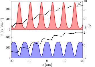
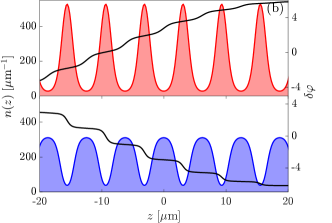
Figure S1: Phase variation of the superfluid Goldstone branches at $k_{z}d/\pi\approx 0.10$. The ground state is shown in solid colors for the dipolar component in red, and the nondipolar component in blue. (a) Density superfluid mode and (b) spin superfluid mode.

References

- Ostermann et al. [2016] S. Ostermann, F. Piazza, and H. Ritsch, Spontaneous crystallization of light and ultracold atoms, Phys. Rev. X 6, 021026 (2016).
- Guo et al. [2021] Y. Guo, R. M. Kroeze, B. P. Marsh, S. Gopalakrishnan, J. Keeling, and B. L. Lev, An optical lattice with sound, Nature 599, 211 (2021).
- Chaikin et al. [1995] P. M. Chaikin, T. C. Lubensky, and T. A. Witten, Principles of condensed matter physics, Vol. 10 (Cambridge university press Cambridge, 1995).
- Kittel [2005] C. Kittel, Introduction to solid state physics (John Wiley & sons, inc, 2005).
- Andreev and Lifshitz [1969a] A. Andreev and I. Lifshitz, Quantum theory of defects in crystals, J. Exp. Theo. Phys. 56, 2057 (1969a).
- Chester [1970] G. Chester, Speculations on bose-einstein condensation and quantum crystals, Physical Review A 2, 256 (1970).
- Leggett [1970] A. J. Leggett, Can a solid be” superfluid”?, Physical Review Letters 25, 1543 (1970).
- Boninsegni and Prokof’ev [2012] M. Boninsegni and N. V. Prokof’ev, Colloquium: Supersolids: What and where are they?, Reviews of Modern Physics 84, 759 (2012).
- Tanzi et al. [2019a] L. Tanzi, E. Lucioni, F. Famà, J. Catani, A. Fioretti, C. Gabbanini, R. N. Bisset, L. Santos, and G. Modugno, Observation of a dipolar quantum gas with metastable supersolid properties, Phys. Rev. Lett. 122, 130405 (2019a).
- Böttcher et al. [2019] F. Böttcher, J.-N. Schmidt, M. Wenzel, J. Hertkorn, M. Guo, T. Langen, and T. Pfau, Transient supersolid properties in an array of dipolar quantum droplets, Phys. Rev. X 9, 011051 (2019).
- Chomaz et al. [2019] L. Chomaz, D. Petter, P. Ilzhöfer, G. Natale, A. Trautmann, C. Politi, G. Durastante, R. M. W. van Bijnen, A. Patscheider, M. Sohmen, M. J. Mark, and F. Ferlaino, Long-lived and transient supersolid behaviors in dipolar quantum gases, Phys. Rev. X 9, 021012 (2019).
- Norcia et al. [2021] M. A. Norcia, C. Politi, L. Klaus, E. Poli, M. Sohmen, M. J. Mark, R. N. Bisset, L. Santos, and F. Ferlaino, Two-dimensional supersolidity in a dipolar quantum gas, Nature 596, 357–361 (2021).
- Li et al. [2017] J.-R. Li, J. Lee, W. Huang, S. Burchesky, B. Shteynas, F. Ç. Top, A. O. Jamison, and W. Ketterle, A stripe phase with supersolid properties in spin–orbit-coupled bose–einstein condensates, Nature 543, 91 (2017).
- Putra et al. [2020] A. Putra, F. Salces-Cárcoba, Y. Yue, S. Sugawa, and I. Spielman, Spatial coherence of spin-orbit-coupled bose gases, Physical Review Letters 124, 053605 (2020).
- Watanabe and Brauner [2012] H. Watanabe and T. Brauner, Spontaneous breaking of continuous translational invariance, Phys. Rev. D 85, 085010 (2012).
- Saccani et al. [2012] S. Saccani, S. Moroni, and M. Boninsegni, Excitation spectrum of a supersolid, Phys. Rev. Lett. 108, 175301 (2012).
- Kunimi and Kato [2012] M. Kunimi and Y. Kato, Mean-field and stability analyses of two-dimensional flowing soft-core bosons modeling a supersolid, Phys. Rev. B 86, 060510 (2012).
- Macrì et al. [2013] T. Macrì, F. Maucher, F. Cinti, and T. Pohl, Elementary excitations of ultracold soft-core bosons across the superfluid-supersolid phase transition, Phys. Rev. A 87, 061602 (2013).
- Li et al. [2013] Y. Li, G. I. Martone, L. P. Pitaevskii, and S. Stringari, Superstripes and the excitation spectrum of a spin-orbit-coupled bose-einstein condensate, Phys. Rev. Lett. 110, 235302 (2013).
- Roccuzzo and Ancilotto [2019] S. M. Roccuzzo and F. Ancilotto, Supersolid behavior of a dipolar bose-einstein condensate confined in a tube, Phys. Rev. A 99, 041601 (2019).
- Geier et al. [2023] K. T. Geier, G. I. Martone, P. Hauke, W. Ketterle, and S. Stringari, Dynamics of stripe patterns in supersolid spin-orbit-coupled bose gases, Phys. Rev. Lett. 130, 156001 (2023).
- Blakie et al. [2023] P. B. Blakie, L. Chomaz, D. Baillie, and F. Ferlaino, Compressibility and speeds of sound across the superfluid-to-supersolid phase transition of an elongated dipolar gas, Phys. Rev. Res. 5, 033161 (2023).
- Tanzi et al. [2019b] L. Tanzi, S. Roccuzzo, E. Lucioni, F. Famà, A. Fioretti, C. Gabbanini, G. Modugno, A. Recati, and S. Stringari, Supersolid symmetry breaking from compressional oscillations in a dipolar quantum gas, Nature 574, 382 (2019b).
- Guo et al. [2019] M. Guo, F. Böttcher, J. Hertkorn, J.-N. Schmidt, M. Wenzel, H. P. Büchler, T. Langen, and T. Pfau, The low-energy goldstone mode in a trapped dipolar supersolid, Nature 574, 386 (2019).
- Natale et al. [2019] G. Natale, R. van Bijnen, A. Patscheider, D. Petter, M. Mark, L. Chomaz, and F. Ferlaino, Excitation spectrum of a trapped dipolar supersolid and its experimental evidence, Physical review letters 123, 050402 (2019).
- Tanzi et al. [2021] L. Tanzi, J. G. Maloberti, G. Biagioni, A. Fioretti, C. Gabbanini, and G. Modugno, Evidence of superfluidity in a dipolar supersolid from nonclassical rotational inertia, Science 371, 1162 (2021), https://www.science.org/doi/pdf/10.1126/science.aba4309 .
- Norcia et al. [2022] M. A. Norcia, E. Poli, C. Politi, L. Klaus, T. Bland, M. J. Mark, L. Santos, R. N. Bisset, and F. Ferlaino, Can angular oscillations probe superfluidity in dipolar supersolids?, Phys. Rev. Lett. 129, 040403 (2022).
- Chomaz et al. [2022] L. Chomaz, I. Ferrier-Barbut, F. Ferlaino, B. Laburthe-Tolra, B. L. Lev, and T. Pfau, Dipolar physics: a review of experiments with magnetic quantum gases, Reports on Progress in Physics 86, 026401 (2022).
- Note [1] Note that we have sketched atom displacements in the transverse direction for illustration purposes only. The present work deals exclusively with longitudinal excitations.
- Pitaevskii and Stringari [2016] L. Pitaevskii and S. Stringari, Bose-Einstein Condensation and Superfluidity (Oxford University Press, 2016).
- Hertkorn et al. [2019] J. Hertkorn, F. Böttcher, M. Guo, J. N. Schmidt, T. Langen, H. P. Büchler, and T. Pfau, Fate of the amplitude mode in a trapped dipolar supersolid, Phys. Rev. Lett. 123, 193002 (2019).
- O’Dell et al. [2003] D. H. J. O’Dell, S. Giovanazzi, and G. Kurizki, Rotons in gaseous Bose-Einstein condensates irradiated by a laser, Phys. Rev. Lett. 90, 110402 (2003).
- Santos et al. [2003] L. Santos, G. Shlyapnikov, and M. Lewenstein, Roton-maxon spectrum and stability of trapped dipolar bose-einstein condensates, Physical Review Letters 90, 250403 (2003).
- Chomaz et al. [2018] L. Chomaz, R. M. W. van Bijnen, D. Petter, G. Faraoni, S. Baier, J. H. Becher, M. J. Mark, F. Wächtler, L. Santos, and F. Ferlaino, Observation of roton mode population in a dipolar quantum gas, Nature Physics 14, 442 (2018).
- Petter et al. [2019] D. Petter, G. Natale, R. M. W. van Bijnen, A. Patscheider, M. J. Mark, L. Chomaz, and F. Ferlaino, Probing the roton excitation spectrum of a stable dipolar bose gas, Phys. Rev. Lett. 122, 183401 (2019).
- Hertkorn et al. [2021] J. Hertkorn, J.-N. Schmidt, F. Böttcher, M. Guo, M. Schmidt, K. Ng, S. Graham, H. Büchler, T. Langen, M. Zwierlein, et al., Density fluctuations across the superfluid-supersolid phase transition in a dipolar quantum gas, Physical Review X 11, 011037 (2021).
- Schmidt et al. [2021] J.-N. Schmidt, J. Hertkorn, M. Guo, F. Böttcher, M. Schmidt, K. S. Ng, S. D. Graham, T. Langen, M. Zwierlein, and T. Pfau, Roton excitations in an oblate dipolar quantum gas, Physical Review Letters 126, 193002 (2021).
- Andreev and Lifshitz [1969b] A. Andreev and I. Lifshitz, Sov. Phys. JETP 29, 1107 (1969b).
- Son [2005] D. T. Son, Effective lagrangian and topological interactions in supersolids, Phys. Rev. Lett. 94, 175301 (2005).
- Yoo and Dorsey [2010] C.-D. Yoo and A. T. Dorsey, Hydrodynamic theory of supersolids: Variational principle, effective lagrangian, and density-density correlation function, Phys. Rev. B 81, 134518 (2010).
- Hofmann and Zwerger [2021] J. Hofmann and W. Zwerger, Hydrodynamics of a superfluid smectic, Journal of Statistical Mechanics: Theory and Experiment 2021, 033104 (2021).
- Šindik et al. [2023] M. Šindik, T. Zawiślak, A. Recati, and S. Stringari, Sound, superfluidity and layer compressibility in a ring dipolar supersolid, arXiv preprint arXiv:2308.05981 (2023).
- Politi et al. [2022] C. Politi, A. Trautmann, P. Ilzhöfer, G. Durastante, M. Mark, M. Modugno, and F. Ferlaino, Interspecies interactions in an ultracold dipolar mixture, Physical Review A 105, 023304 (2022).
- Scheiermann et al. [2023] D. Scheiermann, L. A. Peña Ardila, T. Bland, R. N. Bisset, and L. Santos, Catalyzation of supersolidity in binary dipolar condensates, Phys. Rev. A 107, L021302 (2023).
- Bland et al. [2022] T. Bland, E. Poli, L. A. Peña Ardila, L. Santos, F. Ferlaino, and R. N. Bisset, Alternating-domain supersolids in binary dipolar condensates, Phys. Rev. A 106, 053322 (2022).
- Li et al. [2022] S. Li, U. N. Le, and H. Saito, Long-lifetime supersolid in a two-component dipolar bose-einstein condensate, Phys. Rev. A 105, L061302 (2022).
- Halder et al. [2023] S. Halder, S. Das, and S. Majumder, Two-dimensional miscible-immiscible supersolid and droplet crystal state in a homonuclear dipolar bosonic mixture, Physical Review A 107, 063303 (2023).
- Kirkby et al. [2023] W. Kirkby, T. Bland, F. Ferlaino, and R. Bisset, Spin rotons and supersolids in binary antidipolar condensates, arXiv preprint arXiv:2301.08007 (2023).
- Trautmann et al. [2018] A. Trautmann, P. Ilzhöfer, G. Durastante, C. Politi, M. Sohmen, M. J. Mark, and F. Ferlaino, Dipolar quantum mixtures of erbium and dysprosium atoms, Phys. Rev. Lett. 121, 213601 (2018).
- Ravensbergen et al. [2020] C. Ravensbergen, E. Soave, V. Corre, M. Kreyer, B. Huang, E. Kirilov, and R. Grimm, Resonantly interacting fermi-fermi mixture of and , Phys. Rev. Lett. 124, 203402 (2020).
- Durastante et al. [2020] G. Durastante, C. Politi, M. Sohmen, P. Ilzhöfer, M. J. Mark, M. A. Norcia, and F. Ferlaino, Feshbach resonances in an erbium-dysprosium dipolar mixture, Phys. Rev. A 102, 033330 (2020).
- Schäfer et al. [2023] F. Schäfer, Y. Haruna, and Y. Takahashi, Realization of a quantum degenerate mixture of highly magnetic and nonmagnetic atoms, Phys. Rev. A 107, L031306 (2023).
- Ashcroft and Mermin [1976] N. W. Ashcroft and N. D. Mermin, Solid state physics (Cengage Learning, 1976).
-
[54]
Higgs mode: https://youtu.be/8fKY_LEucBE
Optical mode: https://youtu.be/xL5SxIH7Wgk
Acoustic mode: https://youtu.be/2udOWSJCNeA. - Blakie et al. [2020a] P. B. Blakie, D. Baillie, and S. Pal, Variational theory for the ground state and collective excitations of an elongated dipolar condensate, Communications in Theoretical Physics 72, 085501 (2020a).
- Note [2] Note that a miscible supersolid phase is expected in the bottom right corner of the phase diagram [44, 45] (not shown), which is not the focus of the present work.
- Abad and Recati [2013] M. Abad and A. Recati, A study of coherently coupled two-component bose-einstein condensates, The European Physical Journal D 67, 1 (2013).
- Symes et al. [2014] L. Symes, D. Baillie, and P. Blakie, Static structure factors for a spin-1 bose-einstein condensate, Physical Review A 89, 053628 (2014).
- Chalopin et al. [2020] T. Chalopin, T. Satoor, A. Evrard, V. Makhalov, J. Dalibard, R. Lopes, and S. Nascimbene, Probing chiral edge dynamics and bulk topology of a synthetic hall system, Nature Physics 16, 1017 (2020).
- Gupta et al. [2005] S. Gupta, K. W. Murch, K. L. Moore, T. P. Purdy, and D. M. Stamper-Kurn, Bose-einstein condensation in a circular waveguide, Phys. Rev. Lett. 95, 143201 (2005).
- Olson et al. [2007] S. E. Olson, M. L. Terraciano, M. Bashkansky, and F. K. Fatemi, Cold-atom confinement in an all-optical dark ring trap, Phys. Rev. A 76, 061404 (2007).
- Ryu et al. [2007] C. Ryu, M. F. Andersen, P. Cladé, V. Natarajan, K. Helmerson, and W. D. Phillips, Observation of persistent flow of a bose-einstein condensate in a toroidal trap, Phys. Rev. Lett. 99, 260401 (2007).
- Henderson et al. [2009] K. Henderson, C. Ryu, C. MacCormick, and M. G. Boshier, Experimental demonstration of painting arbitrary and dynamic potentials for bose–einstein condensates, New Journal of Physics 11, 043030 (2009).
- Tengstrand et al. [2021] M. N. Tengstrand, D. Boholm, R. Sachdeva, J. Bengtsson, and S. M. Reimann, Persistent currents in toroidal dipolar supersolids, Phys. Rev. A 103, 013313 (2021).
- Nilsson Tengstrand et al. [2023] M. Nilsson Tengstrand, P. Stürmer, J. Ribbing, and S. M. Reimann, Toroidal dipolar supersolid with a rotating weak link, Phys. Rev. A 107, 063316 (2023).
- Blakie et al. [2020b] P. Blakie, D. Baillie, L. Chomaz, and F. Ferlaino, Supersolidity in an elongated dipolar condensate, Physical Review Research 2, 043318 (2020b).