Design-based inference for generalized network experiments with stochastic interventions

Abstract

A growing number of scholars and data scientists are conducting randomized experiments to analyze causal relationships in network settings where units influence one another. A dominant methodology for analyzing these network experiments has been design-based, leveraging randomization of treatment assignment as the basis for inference. In this paper, we generalize this design-based approach so that it can be applied to more complex experiments with a variety of causal estimands with different target populations. An important special case of such generalized network experiments is a bipartite network experiment, in which the treatment assignment is randomized among one set of units and the outcome is measured for a separate set of units. We propose a broad class of causal estimands based on stochastic intervention for generalized network experiments. Using a design-based approach, we show how to estimate the proposed causal quantities without bias, and develop conservative variance estimators. We apply our methodology to a randomized experiment in education where a group of selected students in middle schools are eligible for the anti-conflict promotion program, and the program participation is randomized within this group. In particular, our analysis estimates the causal effects of treating each student or his/her close friends, for different target populations in the network. We find that while the treatment improves the overall awareness against conflict among students, it does not significantly reduce the total number of conflicts.

Keywords: bipartite network experiment; partial interference; peer effects; randomized experiment; spillover effects

1 Introduction

In randomized experiments across the health and social sciences, units routinely interact with one another. This often leads to the phenomenon of interference where the outcome of one unit is influenced by the treatments assigned to other units (e.g., Halloran and Struchiner 1995; Nickerson 2008; Gupta et al. 2019). Even when analyzing such complex experiments, the randomization of treatment assignment is under the control of the investigator and hence can serve as a “reasoned basis” for statistical inference (Fisher 1935). This explains why the design-based or randomization-based inference has been a dominant approach to analyzing randomized experiments under interference (e.g., Rosenbaum 2007; Hudgens and Halloran 2008; Aronow and Samii 2017; Athey et al. 2018).

A strand of literature has developed design-based approaches for analyzing randomized experiments under clustered network or partial interference where the outcome of one unit can be influenced by the treatment condition of other units but only within the same cluster of units (e.g., Rosenbaum 2007; Hudgens and Halloran 2008; Liu and Hudgens 2014; Imai et al. 2021; Park and Kang 2022). Existing methods, however, can only be applied to experiments where all units in the network are eligible to receive the treatment. This restriction represents an important limitation because many modern network experiments involve some units that are not eligible for treatment assignment or outcome measurement. A prominent example is bipartite network experiments, where treatment is randomized among one set of units while the outcome is measured for a separate set of units (Doudchenko et al. 2020; Harshaw et al. 2021; Zigler and Papadogeorgou 2021).

In addition, although the existing methods focus on the average treatment effect among all treatment-eligible units, researchers may be interested in estimating causal effects for different target populations, such as treatment-ineligible units or a group that includes some of both treatment eligible and ineligible units. For instance, in experiments on ride-sharing platforms such as Uber and Lyft, the treatment (e.g., price discount) may be applied only to riders while analysts wish to estimate causal effects separately for riders and drivers (Bajari et al. 2023). In our motivating application (Paluck et al. 2016), one question of interest is how popular students’ participation in an anti-bullying program can influence the attitudes and behavior of their close friends who are ineligible for the program.

In this paper, we propose a design-based causal inference framework and methodology for generalized network experiments, where an arbitrary subset of units are eligible to receive the treatment and a target population of interest may include both treatment-eligible and ineligible units. Importantly, our framework does not make parametric assumptions nor imposes restrictions on the interference structure.

As our motivating application, we reanalyze an influential randomized clustered network experiment (Paluck et al. 2016). Its original analysis relied on a parametric regression model to investigate whether or not administering an anti-conflict promotion program to a group of students in New Jersey public middle schools, who have many friends, can lead to improved behavior and attitudes among all students in the school (see Section 2). In contrast, while the treatment assignment was randomized only within this group of popular students, we develop and apply a non-parametric estimator to examine the impact of the anti-conflict promotion program on all the students and separately among eligible and ineligible students. Our analysis, therefore, is able to separately estimate peer effects among different groups of students. Moreover, unlike the original analysis quantifies how students’ conflict behaviors are influenced by their own intervention status or that of their close friends.

As an important special case, generalized network experiments encompass bipartite network experiments, where treatment is randomized among one set of units while the outcome is measured for a separate set of units. Bipartite network experiments are often used in two-sided markets where, for example, a price discount (treatment) is administered to a group of products (eligible units) whereas the amount purchased (outcome) is measured on buyers (ineligible units). Although several scholars have recently proposed methods for analyzing bipartite network experiments (Doudchenko et al. 2020; Harshaw et al. 2021; Zigler and Papadogeorgou 2021), they are not fully design-based and are not applicable to other types of generalized network experiments, such as the school conflict experiment by Paluck et al. (2016).

Specifically, we first propose a broad class of causal estimands for generalized network experiments based on stochastic interventions, which represent a hypothetical probabilistic treatment assignment mechanism on the treatment-eligible units (Section 3). Under our framework, one can specify a stochastic intervention regime that assigns the treatment to each unit with different probabilities. This allows us to formalize unit-level causal quantities under different treatment assignment mechanisms. The proposed class of estimands extends the existing definitions of average direct, indirect, and total effects to arbitrary target populations in the network (Hudgens and Halloran 2008; Zigler and Papadogeorgou 2021). These target populations may correspond to, for example, all treatment-eligible units, all treatment-ineligible units, all the units, or units defined by a set of covariates.

Second, we propose Horvitz-Thompson and Hájek estimators for each causal estimand and develop design-based inferential approaches (Section 4). In particular, we show that the Horvitz-Thompson estimator is unbiased in finite samples whereas the Hájek estimator is unbiased in large samples. Moreover, we obtain closed-form expressions for the design-based variances of these estimators. We show that under certain assumptions about the structure of interference, it is possible to obtain conservative estimators of these variances. Our simulation study finds that the Hájek estimator systematically produces more efficient estimates when compared to the Horvitz-Thompson estimators across different simulation settings (Section 5).

Finally, we apply our framework and methodology to the aforementioned experimental study concerning the causal effects of the anti-conflict program (Section 6). As noted above, the original analysis focused on understanding whether encouraging a group of students to take a public stance against conflict (i.e., treatment) can shift overall levels of conflict behavior in schools. Our analysis, instead, examines whether and to what extent the behavior of students is influenced by their own treatment status or the treatment of their close friends. This alternative question is of interest because for any given student, their own treatment status and that of their close eligible friend are more likely to influence their behavior towards conflict, when compared to the treatment status of the other students. We find that intervening on their close friends and themselves improves students’ awareness and overall stance against conflict, while it does not significantly reduce the number of conflict cases in schools, on average.

Related literature.

There exists extensive literature on causal inference with interference (see Tchetgen and VanderWeele 2012; Halloran and Hudgens 2016, for earlier reviews). The most commonly analyzed experimental design in this literature is two-stage randomization. Building on the seminal work by Hudgens and Halloran (2008), many scholars have developed and applied methods to estimate various direct and spillover effects (e.g., Sinclair et al. 2012; Crépon et al. 2013; Liu and Hudgens 2014; Baird et al. 2018; Basse and Feller 2018; Imai et al. 2021). Similar to this literature, we allow general network interference within each cluster, but unlike two-stage randomized designs, we consider the possible existence of treatment-ineligible units and a broader class of spillover effects.

Beyond this specific experimental design, Aronow and Samii (2017) propose an exposure mapping approach by assuming that the potential outcome of one unit depends on the treatment assignments of other units in a network only through a known low-dimensional function of the treatment assignments (Toulis and Kao 2013; Leung 2020). In practice, however, it is often impossible to observe all the ways in which units interact with one another. As a result, the assumptions that severely restrict the structure of interference may be difficult to justify. We take an alternative approach based on stochastic interventions that avoid the specification of an exposure map while maintaining the interpretability of empirical findings. For variance estimation, however, we also assume a certain form of interference as done in the previous works that analyze randomized experiments under interference.

Our work also contributes to the fast growing literature on bipartite network experiments. There are two basic approaches. First, a series of recent works build upon the aforementioned exposure mapping approach under bipartite settings. Under a linear exposure map, Pouget-Abadie et al. (2019) develop a clustering algorithm for estimating the global average treatment effect, i.e., the average effect of treating all eligible units. In addition, under an arbitrary but known exposure map, Doudchenko et al. (2020) show how to estimate the global average treatment effect using regression and weighting methods based on generalized propensity scores. More recently, Harshaw et al. (2021) assume a linear model for both the exposure and the response to estimate the global average treatment effect and develop an inferential approach using asymptotic approximations. Lastly, Yu et al. (2022) and Zhang and Imai (2023) take the middle road by imposing semiparametric assumptions. As mentioned above, we do not adopt the exposure mapping approach in order to avoid, whenever possible, restrictions on the structure of interference.

The second approach to bipartite network experiments is based on stochastic intervention. Zigler and Papadogeorgou (2021) introduce this alternative approach. While they formulate a set of estimands using stochastic interventions, and propose Horvitz-Thompson-type estimators for these estimands, the authors do not consider formal variance estimation. Building on this seminal work, we generalize their estimands and develop design-based assumption-lean inference.

We also contribute to the recent literature on stochastic interventions. Two-stage randomization discussed above can be seen as an application of stochastic intervention. More recently, stochastic interventions have been used in a variety of settings, including causal inference in longitudinal studies (Kennedy 2019), mediation analysis (Díaz and Hejazi 2019), analysis of spatio-temporal data (Papadogeorgou et al. 2020), and other types of observational studies (e.g., Muñoz and Van Der Laan 2012; Young et al. 2014; Papadogeorgou et al. 2019; Zigler et al. 2020). We further extend stochastic interventions to generalized network experiments.

Finally, another related literature focuses on the design and analysis of spatial experiments. In particular, Wang et al. (2020) define causal estimands by considering a circle-average outcome for each treatment-eligible point in space by focusing on Bernoulli assignments (see also Wang 2021). In contrast, the outcomes and estimands in our framework are defined at the level of both eligible and ineligible units and allow for arbitrary assignment mechanisms.

2 Effectiveness of anti-conflict interventions in schools

In this section, we introduce the clustered network experiment analyzed later in the paper and discuss the substantive questions that motivate our proposed methodology.

2.1 Background

An important question in the behavioral and social sciences is whether and how a change in the attitude and behavior of a few individuals can be transmitted through social networks to induce community-wide changes. Paluck et al. (2016) conducted an innovative experimental design to study this question in the context of school conflicts, such as bullying, harassment, and other antagonistic interactions among students. A primary goal of the study was to identify influential students who can effectively change the norms and behavior of other students in the same school.

The authors conducted a randomized experiment across 56 public middle schools in New Jersey, of which 28 were randomly selected for an anti-conflict intervention (i.e., treatment). This intervention program was designed to encourage participating students to take a public stance against school conflicts. In each treated school, a group of students (called “seed-eligible students”) was selected non-randomly. Many of these students were popular in that they reported having many friends within their schools. On average, there were about 50 seed-eligible students and 200 ineligible students in each school. Among the seed-eligible students, half of them (“seed students”) were randomly selected within a pre-defined stratum to participate in the anti-conflict intervention program. In addition, based on the number of social connections among students in each school, a group of highly connected seed students (“referent students”) were identified. On average, there were about five referent students per treated school.

A pre-experimental survey was conducted to collect student-level baseline data on demographic characteristics, social connections, and conflict behaviors and perceptions. In particular, each student reported up to 10 close friends that they spent time with in the last few weeks. Post-experiment data were also collected using a similar survey conducted at the end of the school year, along with the schools’ administrative records. The outcome variables measured awareness about conflict (e.g., whether students wore anti-conflict wristbands) and instances of conflict (e.g., number of cases of conflict).

2.2 Motivating questions

The authors of the original study were primarily interested in comparing the treated and control schools to estimate the causal effects of the intervention at the school level. To this end, the authors conducted a model-based analysis by fitting a linear regression model of school-level outcomes (e.g., number of cases of conflict) on school-level characteristics (e.g., proportion of referent students) and treatment status.

Another key part of the original analysis focused on the effect of treating referent students on all the students in their social network. Specifically, in the population of all the students in the network, the authors estimated the average causal effects of a new quaternate (four-level) treatment — (i) having a seeded friend who is also a referent, (ii) having a seeded friend but no referent friends, (iii) being in a treated school but having no seeded friends, and (iv) being in a control school. Estimation was done using a covariate-adjusted inverse probability weighted regression model with student-level data, and randomization-based inference was performed under the sharp null hypothesis of constant treatment effects. The authors found that, in terms of peer-to-peer social influence, exposure to referent students increases awareness and perceived social norms against conflict, but it does not decrease instances of conflict.

In this paper, we provide an alternative approach to analyzing this experiment. Our analysis differs from that of Paluck et al. (2016) in terms of the causal questions, the target populations, and the mode of estimation and inference.

First, unlike the original analysis, the causal questions in our analysis focus on how students’ conflict behaviors are influenced by their own treatment status or that of their close friends, where closeness is determined by the information provided in the baseline survey. As alluded to earlier, such questions are relevant because a student’s behavior is likely to be dictated by themselves and their close friends, when compared to other students in their school. We also examine whether, after taking into account the influence of close friends, the students’ conflict behaviors are further affected by the referent students who are highly connected seed students.

Our proposed framework embeds these questions into a direct and indirect effects estimation problem under generalized network experiments (see Section 3). A critical component of our framework is the notion of a key-intervention unit. For any unit in a network, its key-intervention units refer to one or more treatment-eligible units whose influence is of particular interest. For instance, in this experiment, the key-intervention units of a seed-eligible student may be themselves, while the key-intervention units of a seed-ineligible student may be their closest seed-eligible friends. The idea of a single key-intervention unit was introduced in Zigler and Papadogeorgou (2021) for bipartite experiments. We extend this notion by enabling multiple units to serve as key-intervention units under generalized network experiments.

Second, the original analysis focuses on estimating the average treatment effect on all the students within a school. In contrast, our analysis separately estimates causal effects for seed-eligible and seed-ineligible students. The effects may vary between these two populations because the seed-eligible students are non-randomly selected and hence their characteristics differ. Moreover, since the seed-ineligible students never receive the treatment, the effects of seed-eligible students’ program participation on these students can be interpreted as peer effects. By comparing the average effects between these two target populations, we can examine the extent to which the treatment effect transmits from eligible students to their ineligible peers through their friendship network.

Finally, the authors of the original study used both model-based and design-based approaches. In their model-based analysis, the inferential validity relies on the appropriateness of the assumed regression models. In contrast, our analyses are fully design-based and hence, do not require modeling assumptions. In their design-based analysis, the uncertainty quantification relies upon the assumption of constant additive treatment effects. We address this limitation by providing design-based confidence intervals for the causal effects of interest while allowing for heterogeneous treatment effects.

3 Methodological framework for generalized network experiments

3.1 Setup and notation

Consider a generalized network experiment on a finite population comprising a set of treatment-eligible or intervention units $\mathcal{I}$ (e.g., seed-eligible students in our application) and a set of treatment-ineligible or non-intervention units $\mathcal{O}$ (e.g., seed-ineligible students), grouped into $K(\geq 1)$ non-overlapping clusters (e.g., schools). We write $\mathcal{I}=\mathcal{I}_{1}\cup...\cup\mathcal{I}_{K}$ and $\mathcal{O}=\mathcal{O}_{1}\cup...\cup\mathcal{O}_{K}$, where $\mathcal{I}_{k}$ and $\mathcal{O}_{k}$ denote the sets of $n_{k}$ intervention units and $m_{k}$ non-intervention units in cluster $k$, respectively. Here, $\mathcal{I}_{k}$ and $\mathcal{O}_{k}$ are disjoint. Denote $\mathcal{S}_{k}\subseteq\mathcal{I}_{k}\cup\mathcal{O}_{k}$ as the target population of interest in cluster $k$ for which we wish to learn certain causal effects of the intervention. Finally, we use $\mathcal{S}=\mathcal{S}_{1}\cup\mathcal{S}_{2}\cup...\cup\mathcal{S}_{K}$ to denote the combined target population across all clusters.

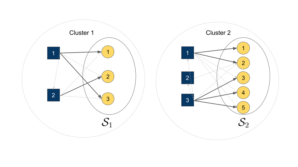
Figure 1: An example of a generalized network experiment with two clusters. A directed arrow from an intervention unit (blue square) to a non-intervention unit (yellow circle) indicates that the treatment received by the intervention unit may causally affect the outcome of the non-intervention unit. For each non-intervention unit, solid arrows correspond to the key-intervention units and the dashed arrows correspond to other intervention units. For each intervention unit, the corresponding key-intervention unit is itself. Here, the target population is the set of non-intervention units.

Figure 1 presents an example with $K=2$ clusters. The intervention units are represented by blue squares whereas the non-intervention units are yellow circles. A directed arrow denotes a potential causal effect of an intervention unit’s treatment on the outcome of another unit, which may or may not be eligible for the treatment. Here, the target population is the set of non-intervention units.

With different choices of population $\mathcal{S}$, this setup encompasses other common network experiment designs as illustrated in the following examples.

Example 1 (Standard clustered network experiments).

$\mathcal{S}_{k}=\mathcal{I}_{k}$, where inferences are made for the units that can be assigned to either the treatment or control condition.

Example 2 (Bipartite experiments).

$\mathcal{S}_{k}=\mathcal{O}_{k}$, where inferences are made for the units that are not eligible to receive treatment.

Example 3.

$\mathcal{S}_{k}=\mathcal{I}_{k}\cup\mathcal{O}_{k}$, where inferences are made for the overall population of units.

In addition, $\mathcal{S}_{k}$ may correspond to a population characterized by covariates. For instance, in the school conflict experiment, the population of interest may be all the female students or all students who were involved in at least one case of conflict before the experiment took place.

Next, let $\bm{A}_{k}=(A_{ki}:i\in\mathcal{I}_{k})$ denote the vector of treatment assignment indicators in cluster $k$, with $A_{ki}=1$ if intervention unit $i\in\mathcal{I}_{k}$ receives the treatment, and $A_{ki}=0$ otherwise. Also, we measure $d$ baseline covariates for each unit in cluster $k$. Define $\bm{X}_{k}\in\mathbb{R}^{d(n_{k}+m_{k})}$ as the stacked vector of observed covariates across all the units in cluster $k$, and write $\mathcal{X}=\{\bm{X}_{1},...,\bm{X}_{K}\}$. For each unit $j\in\mathcal{S}_{k}$, let $Y_{kj}(\bm{a}_{1},...,\bm{a}_{K})$ represent its potential outcome (e.g., the number of conflict incidents) when the vectors of treatment levels in clusters $1,2,...,K$ equal $\bm{a}_{1},\bm{a}_{2},...,\bm{a}_{K}$, respectively. We use $\mathcal{Y}=\{Y_{kj}(\bm{a}_{1},...,\bm{a}_{K}):\bm{a}_{k}\in\{0,1\}^{n_{k}},j\in\mathcal{S}_{k},k\in\{1,...,K\}\}$ to represent the set of all possible potential outcomes across all units in $\mathcal{S}$. Finally, for $j\in\mathcal{S}_{k}$, let $Y^{\text{obs}}_{kj}=Y_{kj}(\bm{A}_{1},...,\bm{A}_{K})$ be the corresponding observed outcome.

Throughout the paper, we adopt a finite population causal inference framework (Neyman 1923, 1990), where the sets of potential outcomes $\mathcal{Y}$ and the covariates $\mathcal{X}$ are fixed and randomness stems from the treatment assignments ($\bm{A}_{1},...,\bm{A}_{K}$) alone. Furthermore, we assume that the potential outcomes of each unit in a cluster may depend on the treatments assigned to any intervention unit in the same cluster but do not depend on the treatment assignments of units in other clusters.

Assumption 1 (Partial interference (Sobel 2006; Hudgens and Halloran 2008)).

For all $k\in\{1,2,...,K\}$ and $j\in\mathcal{I}_{k}\cup\mathcal{O}_{k}$, $Y_{kj}(\bm{a}_{1},...,\bm{a}_{K})=Y_{kj}(\bm{a}^{\prime}_{1},...,\bm{a}^{\prime}_{K})$ if $\bm{a}_{k}=\bm{a}^{\prime}_{k}$. ∎

Assumption 1 allows for interference within each cluster, but rules out interference across clusters. In our application, the assumption implies that students do not influence one another across schools. Under this assumption, we can write $Y_{kj}(\bm{a}_{k})=Y_{kj}(\bm{a}_{1},...,\bm{a}_{K})$ for all $k\in\{1,2,...,K\}$ and $j\in\mathcal{S}_{k}$. Assumption 1 can be relaxed by positing $Y^{\text{obs}}_{kj}=Y_{kj}(\bm{A}_{\mathcal{K}})$ where $\mathcal{K}$ is a collection of the clusters that includes cluster $k$, i.e., $\mathcal{K}\subset\{1,2.,...,K\}$ and $k\in\mathcal{K}$. When $K=1$ (i.e., the experiment is conducted in a single cluster), the assumption holds trivially.

Finally, for each unit $j$ in cluster $k$, denote $i^{*}=i^{*}(j)\in\mathcal{I}_{k}$ as its key intervention unit (Zigler and Papadogeorgou 2021). The key-intervention unit is often of particular interest as they are likely to influence the behavior of the corresponding non-intervention unit. For example, in our application, the key intervention unit of a seed-eligible student may be themselves, while the key-intervention unit of a seed-ineligible student may be the best friend of the student. We can directly incorporate the role of the key-intervention unit in the definition of causal estimands, as shown below.

3.2 Estimands

Under the setup described above, we define a broad class of causal estimands for generalized network experiments using stochastic interventions, extending the existing estimands in the literature.

3.2.1 The general formulation

For any unit $j\in\mathcal{S}_{k}$, we consider a stochastic intervention $\pi_{kj}(\cdot\mid\mathcal{X}):\{0,1\}^{n_{k}}\to[0,1]$ on the intervention units in cluster $k$. In other words, $\pi_{kj}(\cdot\mid\mathcal{X})$ is a probability distribution over all possible treatment assignments on the units in $\mathcal{I}_{k}$, which may depend on unit $j$ and the set of covariates $\mathcal{X}$. For notational simplicity, in the remainder of this paper, we omit conditioning on the covariates and write $\pi_{kj}(\cdot)$.

Our proposed causal estimand formalizes the notion of target population average potential outcome, where for each unit $j\in\mathcal{S}_{k}$, treatments are assigned to the units in $\mathcal{I}_{k}$ using the assignment mechanism $\pi_{kj}(\cdot)$. The formal definition is given by,

$$\tau^{\pi}=\frac{1}{K}\sum_{k=1}^{K}\left[\frac{1}{|\mathcal{S}_{k}|}\sum_{j\in\mathcal{S}_{k}}\left\{\sum_{\bm{a}\in\{0,1\}^{n_{k}}}\pi_{kj}(\bm{a})Y_{kj}(\bm{a})\right\}\right].$$ (1)

This estimand involves averaging at three levels. First, for each unit $j\in\mathcal{S}_{k}$, the potential outcomes $Y_{kj}(\bm{a})$ are averaged over all possible assignments $\bm{a}$ of the intervention units according to $\pi_{kj}(\cdot)$. Second, these unit-level average potential outcomes are further averaged over all units in $\mathcal{S}_{k}$ to obtain cluster-level average potential outcomes. Finally, they are averaged over all the clusters to obtain the target population average potential outcome.

In this paper, we focus on a subclass of the above general estimand. In particular, for each $j\in\mathcal{S}_{k}$, let $\mathcal{C}_{kj}\subseteq\{0,1\}^{n_{k}}$ denote the set of design-admissible treatment assignments for the corresponding intervention units. For instance, $\mathcal{C}_{kj}=\{\bm{a}\in\{0,1\}^{n_{k}}:A_{ki^{*}}=1\}$ corresponds to the subset of possible treatment assignments where the key-intervention unit $i^{*}$ of unit $j$ receives the treatment. The subclass of estimands is created by setting $\pi_{kj}(\cdot)=\pi_{k}(\cdot\mid\mathcal{C}_{kj})$, where $\pi_{k}(\cdot)$ is a probability distribution, free of $j$. For the school conflict experiment with $\mathcal{S}_{k}=\mathcal{O}_{k}$, we can interpret the resulting estimand $\tau^{\pi}$ as the target population average potential outcome (e.g., the average number of conflicts in all schools) where, for each seed-ineligible student $j$ in school $k$, the seed-eligible students in cluster $k$ receive the intervention with probability $\pi_{k}(\cdot)$, restricted to the set of design-admissible assignments $\mathcal{C}_{kj}$.

3.2.2 Effects of a single key-intervention unit

Using $\tau^{\pi}$, we can encapsulate several practically relevant causal estimands as special cases, including the direct, indirect, and total effects in standard network experiments (Hudgens and Halloran 2008) and bipartite experiments (Zigler and Papadogeorgou 2021). To see this, we first set $\mathcal{C}_{kj}=\{\bm{a}\in\{0,1\}^{n_{k}}:A_{ki^{*}}=a\}$ where $a\in\{0,1\}$ and note that $\tau^{\pi}$ can be written as,

$$\mu^{\pi}_{a}=\frac{1}{K}\sum_{k=1}^{K}\left[\frac{1}{|\mathcal{S}_{k}|}\sum_{j\in\mathcal{S}_{k}}\left\{\sum_{\bm{s}}\pi_{k}(\bm{A}_{k(-i^{*})}=\bm{s}\mid A_{ki^{*}}=a)Y_{kj}(A_{ki^{*}}=a,\bm{A}_{k(-i^{*})}=\bm{s})\right\}\right].$$ (2)

In the school conflict experiment, setting $\mathcal{S}_{k}=\mathcal{O}_{k}$, $\mu^{\pi}_{a}$ represents the average potential outcome when in each school $k$, the best seed-eligible friend of each seed-ineligible student is assigned to the treatment condition $a\in\{0,1\}$, while the treatment assignment for all the other seed-eligible students in the school follows the distribution $\pi_{k}(\cdot)$.

Using the definition of $\mu^{\pi}_{a}$ above, we can write the direct effect as follows,

$$\text{DE}^{\pi}=\mu^{\pi}_{1}-\mu^{\pi}_{0}.$$ (3)

In the school conflict experiment, setting $\mathcal{S}_{k}=\mathcal{O}_{k}$, $\text{DE}^{\pi}$ can be interpreted as the average effect of treating the best seed-eligible friend of every seed-ineligible student, letting the treatment assignment of all the other seed-eligible students in the school $k$ follow $\pi_{k}(\cdot)$. In this case, $\text{DE}^{\pi}$ equals the existing definition of the direct effect in bipartite experiments (Zigler and Papadogeorgou 2021). Likewise, for $\mathcal{S}_{k}=\mathcal{I}_{k}$, $\text{DE}^{\pi}$ is equivalent to the existing definition of the direct effect in standard network experiments (Hudgens and Halloran 2008).

For a fixed treatment level $a\in\{0,1\}$, we can also formalize the indirect effect as

$$\text{IE}^{\pi,\tilde{\pi}}_{a}=\mu^{\pi}_{a}-\mu^{\tilde{\pi}}_{a},$$ (4)

where $\tilde{\pi}_{k}(\cdot):\{0,1\}^{n_{k}}\to[0,1]$ is another stochastic intervention on the intervention units in cluster $k$. For $\mathcal{S}_{k}=\mathcal{O}_{k}$, $\text{IE}^{\pi,\tilde{\pi}}_{a}$ can be interpreted as the average effect of changing the treatment assignment mechanism of all but the best seed-eligible friend of every seed-ineligible student in school $k$ from $\tilde{\pi}_{k}(\cdot)$ to $\pi_{k}(\cdot)$, holding the treatment level of the best-seed eligible friend fixed at $a$. Here, $\pi_{k}(\cdot)$ to $\tilde{\pi}_{k}(\cdot)$ may correspond to assignment mechanisms where we treat a higher proportion of referent students in one and a lower proportion in the other. Once again, this definition extends existing notions of indirect effect to generalized network experiments.

We can also contrast the treatment status of the key-intervention unit and two different stochastic interventions simultaneously to define an average total effect.

$$\text{TE}^{\pi,\tilde{\pi}}=\mu^{\pi}_{1}-\mu^{\tilde{\pi}}_{0},$$ (5)

For $\mathcal{S}_{k}=\mathcal{O}_{k}$, $\text{TE}^{\pi,\tilde{\pi}}$ can be interpreted as the average effect of providing the treatment to the best seed-eligible friend of every seed-ineligible student in school $k$, while changing the treatment assignment mechanism of the other seed-eligible students from $\tilde{\pi}_{k}(\cdot)$ to $\pi_{k}(\cdot)$.

3.2.3 Effects of multiple key-intervention units

In addition, $\tau^{\pi}$ can also incorporate causal quantities based on multiple key-intervention units. For example, we can define the average potential outcome under a stochastic intervention that intervenes on a fixed proportion (e.g., 0.5) of the seed-eligible friends of a student. To formalize, for unit $j\in\mathcal{S}_{k}$, denote $\bm{i}^{*}=\{i^{*}_{1},...,i^{*}_{r_{j}}\}$ as the corresponding set of $r_{j}$ seed-eligible key-intervention units. With multiple key-intervention units, an analog of $\mu^{\pi}_{a}$ can be obtained by setting $\mathcal{C}_{kj}=\{\bm{a}\in\{0,1\}^{n_{k}}:A_{ki^{*}_{s}}=a,s\in\{1,...,r_{j}\}\}$. More generally, we can set $\mathcal{C}_{kj}=\{\bm{a}\in\{0,1\}^{n_{k}}:\sum_{s=1}^{r}A_{ki^{*}_{s}}/r_{j}=p^{*}\}$, where $p^{*}\in[0,1]$. In this case, $\tau^{\pi}$ represents the target population average potential outcome under the intervention mechanism $\pi_{k}(\cdot)$, while fixing, for each unit in $\mathcal{S}_{k}$, the proportion of treated key-intervention units to $p^{*}$.

3.3 Nonparametric identification and estimation

Let $f(\cdot\mid\mathcal{X})$ and $f_{k}(\cdot\mid\mathcal{X})$ denote the joint distributions of the assignment mechanisms in the overall population and in cluster $k$, respectively. Unless otherwise specified, for notational simplicity, we omit conditioning on the covariates. The proposed estimand $\tau^{\pi}$ in Equation (1) can be non-parametrically identified under the following assumptions.

Assumption 2 (Identification of $\tau^{\pi}$).

2. Overlap: For all $k\in\{1,2,...,K\}$, $\text{Supp}(\pi_{kj})\subseteq\text{Supp}(f_{k})$.

3. Unconfoundedness: For all $k\in\{1,2,...,K\}$ and for all $\bm{a}\in\{0,1\}^{n_{k}}$, $f_{k}(\bm{a}\mid\mathcal{X},\mathcal{Y})=f_{k}(\bm{a}\mid\mathcal{X})$.

∎

Assumption 2(a) states that any treatment assignment that has a strictly positive probability under the stochastic intervention of interest $\pi_{kj}(\cdot)$ also has a strictly positive probability under the actual intervention $f_{k}(\cdot)$. This is analogous to the positivity or overlap assumption in observational studies. Assumption 2(b) is equivalent to the usual unconfoundedness assumption in observational studies and states that conditional on the covariates, the assignment mechanism does not depend on the potential outcomes. In randomized experiments, this assumption is satisfied by design.

Under Assumption 2, we can nonparametrically identify $\tau^{\pi}$ as

$$\tau^{\pi}=\frac{1}{K}\sum_{k=1}^{K}\left[\frac{1}{|\mathcal{S}_{k}|}\sum_{j\in\mathcal{S}_{k}}\mathbb{E}\left\{\sum_{\bm{a}\in\{0,1\}^{n_{k}}}\mathbbm{1}(\bm{A}_{k}=\bm{a})\frac{\pi_{kj}(\bm{a})}{f_{k}(\bm{a})}Y^{\text{obs}}_{kj}\right\}\right].$$ (6)

This identification result suggests the following Horvitz-Thompson-type weighted estimator of $\tau^{\pi}$,

$$\hat{\tau}^{\pi}_{\text{HT}}=\frac{1}{K}\sum_{k=1}^{K}\left\{\frac{1}{|\mathcal{S}_{k}|}\sum_{j\in\mathcal{S}_{k}}\frac{\pi_{kj}(\bm{A}_{k})}{f_{k}(\bm{A}_{k})}Y^{\text{obs}}_{kj}\right\}.$$ (7)

In the special case of $\tau^{\pi}=\mu^{\pi}_{a}$, we obtain,

$$\hat{\tau}^{\pi}_{\text{HT}}=\frac{1}{K}\sum_{k=1}^{K}\left\{\frac{1}{|\mathcal{S}_{k}|}\sum_{j\in\mathcal{S}_{k}}\mathbbm{1}(A_{ki^{*}}=a)\frac{\pi_{k}(\bm{A}_{k(-i^{*})}\mid A_{ki^{*}}=a)}{f_{k}(\bm{A}_{k})}Y^{\text{obs}}_{kj}\right\}=:\hat{\mu}^{\pi}_{a,\text{HT}}.$$ (8)

For bipartite experiments (i.e., $\mathcal{S}_{k}=\mathcal{O}_{k}$), $\hat{\mu}^{\pi}_{a,\text{HT}}$ boils down to the Horvitz-Thompson estimator of $\mu^{\pi}_{a}$ proposed by Zigler and Papadogeorgou (2021).

The theorem below shows that $\hat{\tau}^{\pi}_{\text{HT}}$ is unbiased for $\tau^{\pi}$ under the design-based framework.

Theorem 3.1 (Unbiasedness).

$\mathbb{E}(\hat{\tau}^{\pi}_{\text{HT}})=\tau^{\pi}$, where the expectation is taken over the assignment mechanism $f(\cdot)$.

Theorem 3.1 also suggests the following Hájek-type estimator of $\tau^{\pi}$,

$$\hat{\tau}^{\pi}_{\text{H\'{a}jek}}=\frac{\sum_{k=1}^{K}\left\{\frac{1}{|\mathcal{S}_{k}|}\sum_{j\in\mathcal{S}_{k}}\frac{\pi_{kj}(\bm{A}_{k})}{f_{k}(\bm{A}_{k})}Y^{\text{obs}}_{kj}\right\}}{\sum_{k=1}^{K}\left\{\frac{1}{|\mathcal{S}_{k}|}\sum_{j\in\mathcal{S}_{k}}\frac{\pi_{kj}(\bm{A}_{k})}{f_{k}(\bm{A}_{k})}\right\}},$$ (9)

which replaces the denominator $K$ in $\hat{\tau}^{\pi}_{\text{HT}}$ with its Horvitz-Thompson estimator. In the special case of $\tau^{\pi}=\mu^{\pi}_{a}$, we have,

$$\hat{\tau}^{\pi}_{\text{H\'{a}jek}}=\frac{\sum_{k=1}^{K}\left\{\frac{1}{|\mathcal{S}_{k}|}\sum_{j\in\mathcal{S}_{k}}\mathbbm{1}(A_{ki^{*}}=a)\frac{\pi_{k}(A_{ki^{*}}=a\mid\bm{A}_{k(-i^{*})})}{f_{k}(\bm{A}_{k})}Y^{\text{obs}}_{kj}\right\}}{\sum_{k=1}^{K}\left\{\frac{1}{|\mathcal{S}_{k}|}\sum_{j\in\mathcal{S}_{k}}\mathbbm{1}(A_{ki^{*}}=a)\frac{\pi_{k}(A_{ki^{*}}=a\mid\bm{A}_{k(-i^{*})})}{f_{k}(\bm{A}_{k})}\right\}}=:\hat{\mu}^{\pi}_{\text{H\'{a}jek}}.$$ (10)

Our definition of the Hájek estimators extends existing notions of Hájek estimators under interference (see, e.g., Wang et al. 2020) to general target populations, assignment mechanisms, and stochastic interventions.

While the Hájek estimator is not unbiased for $\tau^{\pi}$ in finite samples, we show that under certain regularity conditions, it is consistent for $\tau^{\pi}$ (see Section 4.2). The direct and indirect effects given in Equations (3) and (4) are estimated analogously by replacing each component term by its Horvitz-Thompson and Hájek estimators.

4 Design-based inference

In this section, we discuss design-based inference based on the estimators outlined in Section 3. We derive the design-based variances of these estimators and obtain closed-form conservative estimators of these variances. After discussing the Horvitz-Thompson estimators of $\mu^{\pi}_{a}$, $\text{DE}^{\pi}$, and $\text{IE}^{\pi}$, we consider the design-based variances of the corresponding Hájek estimators.

4.1 Horvitz-Thompson estimator

4.1.1 The general variance expression and partial identification

Throughout this section, we maintain the partial interference (Assumption 1) and the identification assumptions (Assumption 2). Additionally, we assume that the treatment assignment mechanisms are independent across clusters.

Assumption 3 (Independence of treatment assignment mechanisms across clusters).

$\bm{A}_{1},...,\bm{A}_{K}$ are mutually independent. ∎

We make this assumption to simplify the variance calculations, although it can be relaxed to incorporate dependence among clusters. An example of such dependence includes the use of complete randomization across clusters in two-stage randomized experiments. We note that this assumption is satisfied in the school conflict experiment.

Next, we consider the case of a single key-intervention unit and obtain a closed-form variance expression for $\hat{\mu}^{\pi}_{a,\text{HT}}$. Appendix B.1 in the Supplementary Materials presents the generalization of this result to the case of multiple key-intervention units.

Theorem 4.1 (Variance of the Horvitz-Thompson Estimator).

Under Assumptions 1, 2, and 3,

$${\text{Var}}(\hat{\mu}^{\pi}_{a,\text{HT}})=\frac{1}{K^{2}}\sum_{k=1}^{K}\frac{1}{|\mathcal{S}_{k}|^{2}}\left(\sum_{j\in\mathcal{S}_{k}}\Lambda_{1,kj}+\mathop{\sum\sum}_{j\neq j^{\prime}\in\mathcal{S}_{k}}\Lambda_{2,kj}\right),$$ (11)

where

$$\Lambda_{1,kj}\ =\ \sum_{\bm{s}}\frac{\pi^{2}_{k}(\bm{A}_{k(-i^{*})}=\bm{s}\mid A_{ki^{*}}=a)}{f_{k}(A_{ki^{*}}=a,\bm{A}_{k(-i^{*})}=\bm{s})}Y^{2}_{kj}(A_{ki^{*}}=a,\bm{A}_{k(-i^{*})}=\bm{s})$$

$$\quad-\left\{\sum_{\bm{s}}\pi_{k}(\bm{A}_{k(-i^{*})}=\bm{s}\mid A_{ki^{*}}=a)Y_{kj}(A_{ki^{*}}=a,\bm{A}_{k(-i^{*})}=\bm{s})\right\}^{2},$$ (12)

$$\Lambda_{2,kj}\ =\ \sum_{\bm{s}}\pi_{k}(\bm{A}_{k(-i^{*})}=\bm{s}\mid A_{ki^{*}}=a)\pi_{k}(\bm{A}_{k(-i^{*^{\prime}})}=\bm{s}\mid A_{ki^{*^{\prime}}}=a)$$

$$\quad\times Y_{kj}(A_{ki^{*}}=a,\bm{A}_{k(-i^{*})}=\bm{s})Y_{kj^{\prime}}(A_{ki^{*^{\prime}}}=a,\bm{A}_{k(-i^{*^{\prime}})}=\bm{s})$$

$$\quad\times\frac{\mathbbm{1}(A_{ki^{*}}=a,A_{ki^{*^{\prime}}}=a,\bm{A}_{k(-i^{*})}=\bm{s},\bm{A}_{k(-i^{*^{\prime}})}=\bm{s})}{f_{k}(A_{ki^{*}}=a,\bm{A}_{k(-i^{*})}=\bm{s})}$$

$$-\Big{\{}\sum_{\bm{s}}\pi_{k}(\bm{A}_{k(-i^{*})}=\bm{s}\mid A_{ki^{*}}=a)Y_{kj}(A_{ki^{*}}=a,\bm{A}_{k(-i^{*})}=\bm{s})\Big{\}}$$

$$\times\Big{\{}\sum_{\bm{s}}\pi_{k}(\bm{A}_{k(-i^{*^{\prime}})}=\bm{s}\mid A_{ki^{*^{\prime}}}=a)Y_{kj^{\prime}}(A_{ki^{*^{\prime}}}=a,\bm{A}_{k(-i^{*^{\prime}})}=\bm{s})\Big{\}}.$$ (13)

Here, $i^{*^{\prime}}=i^{*}(j^{\prime})$ is the key-intervention unit of unit $j^{\prime}$.

Theorem 4.1 implies that in general, the variance of $\hat{\mu}^{\pi}_{a,\text{HT}}$ is non-identifiable. To see this, consider the second term in the expression of $\Lambda_{1,kj}$ in Equation (12), which can be further decomposed as follows,

$$\left\{\sum_{\bm{s}}\pi_{k}(\bm{A}_{k(-i^{*})}=\bm{s}\mid A_{ki^{*}}=a)Y_{kj}(A_{ki^{*}}=a,\bm{A}_{k(-i^{*})}=\bm{s})\right\}^{2}$$

$$= \sum_{\bm{s}}\pi^{2}_{k}(\bm{A}_{k(-i^{*})}=\bm{s}\mid A_{ki^{*}}=a)Y^{2}_{kj}(A_{ki^{*}}=a,\bm{A}_{k(-i^{*})}=\bm{s})$$

$$+\mathop{\sum\sum}_{\bm{s}\neq\bm{s}^{\prime}}\pi_{k}(\bm{A}_{k(-i^{*})}=\bm{s}\mid A_{ki^{*}}=a)\pi_{k}(\bm{A}_{k(-i^{*})}=\bm{s}^{\prime}\mid A_{ki^{*}}=a)$$

$$\hskip 36.135pt\times Y_{kj}(A_{ki^{*}}=a,\bm{A}_{k(-i^{*})}=\bm{s})Y_{kj}(A_{ki^{*}}=a,\bm{A}_{k(-i^{*})}=\bm{s}^{\prime}).$$ (14)

The second term of Equation (14) is not identifiable since, for any unit $j$, we cannot observe both $Y_{kj}(A_{ki^{*}}=a,\bm{A}_{k(-i^{*})}=\bm{s})$ and $Y_{kj}(A_{ki^{*}}=a,\bm{A}_{k(-i^{*})}=\bm{s}^{\prime})$ for $\bm{s}\neq\bm{s}^{\prime}$. Therefore, to identify ${\text{Var}}(\hat{\mu}^{\pi}_{a,\text{HT}})$, we need to invoke some additional assumptions on the pattern of interference among the units in the network.

One possible approach is to assume that for a given treatment condition of the key-intervention unit $i^{*}$, if the two assignment vectors of the remaining intervention units are sufficiently similar, then the corresponding potential outcomes of unit $j$ should also be similar. Specifically, within each cluster, we can partially identify ${\text{Var}}(\hat{\mu}^{\pi}_{a,\text{HT}})$ by assuming the following form of Lipschitz continuity on the potential outcomes.

Assumption 4 (Lipschitz potential outcomes).

For all $j\in\mathcal{S}_{k}$ and $\bm{s},\bm{s}^{\prime}\in\{0,1\}^{n_{k}-1}$,

$$|Y_{kj}(A_{ki^{*}}=a,\bm{A}_{k(-i^{*})}=\bm{s})-Y_{kj}(A_{ki^{*}}=a,\bm{A}_{k(-i^{*})}=\bm{s}^{\prime})|\leq C(n_{k})\times d(\bm{s},\bm{s}^{\prime}),$$

where $C(n_{k})$ is a function of $n_{k}$ that decreases to zero as $n_{k}\to\infty$, and $d(\cdot,\cdot)$ is a distance measure on $\mathbb{R}^{n_{k}-1}$. ∎

For example, if $C(n_{k})=c/\sqrt{n_{k}}$ for some constant $c>0$ and $d(\cdot,\cdot)$ is the $L_{1}$ distance, then Assumption 4 implies that $|Y_{kj}(A_{ki^{*}}=a,\bm{A}_{k(-i^{*})}=\bm{s})-Y_{kj}(A_{ki^{*}}=a,\bm{A}_{k(-i^{*})}=\bm{s}^{\prime})|$ is bounded by $c/\sqrt{n_{k}}$ times the number of intervention units for which the treatment assignment vectors $\bm{s}$ and $\bm{s}^{\prime}$ differ.

Proposition 4.2 shows that if the potential outcomes are bounded, then under Assumptions 1–4, we can partially identify ${\text{Var}}(\hat{\mu}^{\pi}_{a,\text{HT}})$ in completely randomized experiments.

Proposition 4.2 (Partial identification of the variance).

Consider a completely randomized experiment in each cluster $k\in\{1,2,...,K\}$, where $n_{ka}$ and $p_{k}$ are the number and proportion of intervention units assigned to treatment $a\in\{0,1\}$, respectively. Under Assumptions 1–4, $\pi_{k}(\cdot)=f_{k}(\cdot)$, and bounded potential outcomes,

$${\text{Var}}(\hat{\mu}^{\pi}_{a,\text{HT}})\ \leq\ \frac{1}{K^{2}}\sum_{k=1}^{K}\frac{1}{|\mathcal{S}_{k}|^{2}}\left[\left\{\frac{C(n_{k})^{2}|\mathcal{S}_{k}|}{2{{n_{k}-1}\choose{n_{ka}-1}}}^{2}+\frac{C(n_{k})^{2}|\mathcal{S}_{k}|(|\mathcal{S}_{k}|-1)}{2{{n_{k}-2}\choose{n_{ka}-2}}^{2}}\right\}\mathop{\sum\sum}_{\bm{s}\neq\bm{s}^{\prime}}d^{2}(\bm{s},\bm{s}^{\prime})\right.$$

$$+\frac{1-p_{k}}{p_{k}{{n_{k}-1}\choose{n_{ka}-1}}}\sum_{j\in\mathcal{S}_{k}}\sum_{\bm{s}}Y^{2}_{kj}(A_{ki^{*}}=a,A_{k(-i^{*})}=\bm{s})$$

$$+\mathop{\sum\sum}_{j\neq j^{\prime}\in\mathcal{S}_{k}}\left(\frac{1}{{{n_{k}-1}\choose{n_{ka}-1}}p_{k}}-\frac{1}{{{n_{k}-2}\choose{n_{ka}-2}}}\right)\sum_{\bm{s}}Y_{kj}(A_{ki^{*}}=a,A_{ki^{*^{\prime}}}=a,A_{k(-i^{*},i^{*^{\prime}})}=\bm{s})$$

$$\phantom{.........................................................}Y_{kj^{\prime}}(A_{ki^{*}}=a,A_{ki^{*^{\prime}}}=a,A_{k(-i^{*},i^{*^{\prime}})}=\bm{s})\Bigg{]}$$ (15)

The upper bound in Equation 15 is estimable. To see this, note that in the second term $\sum_{j\in\mathcal{S}_{k}}\sum_{\bm{s}}Y^{2}_{kj}(A_{ki^{*}}=a,A_{k(-i^{*})}=\bm{s})$ can be estimated by $\sum_{j\in\mathcal{S}_{k}}\frac{\mathbbm{1}(A_{ki^{*}}=a)}{f_{k}(\bm{A}_{k})}Y_{kj}^{2}$ without bias. Moreover, in the last term $\mathop{\sum\sum}_{j\neq j^{\prime}\in\mathcal{S}_{k}}\sum_{\bm{s}}Y_{j}(A_{ki^{*}}=a,A_{ki^{*^{\prime}}}=a,A_{k(-i^{*},i^{*^{\prime}})}=\bm{s})Y_{j^{\prime}}(A_{ki^{*}}=a,A_{ki^{*^{\prime}}}=a,A_{k(-i^{*},i^{*^{\prime}})}=\bm{s})$ can be estimated without bias by $\mathop{\sum\sum}_{j\neq j^{\prime}\in\mathcal{S}_{k}}\frac{\mathbbm{1}(A_{ki^{*}}=a,A_{ki^{*^{\prime}}}=a)}{f_{k}(\bm{A}_{k})}Y_{kj}Y_{kj^{\prime}}$. Therefore, a conservative estimator of ${\text{Var}}(\hat{\mu}^{\pi}_{a,\text{HT}})$ is given by

$$\widehat{{\text{Var}}}(\hat{\mu}^{\pi}_{a,\text{HT}})= \frac{1}{K^{2}}\sum_{k=1}^{K}\frac{1}{|\mathcal{S}_{k}|^{2}}\left[\left\{\frac{C(n_{k})^{2}|\mathcal{S}_{k}|}{{{n_{k}-1}\choose{n_{ka}-1}}}+\frac{C(n_{k})^{2}|\mathcal{S}_{k}|(|\mathcal{S}_{k}|-1)}{2{{n_{k}-2}\choose{n_{ka}-2}}^{2}}\right\}\mathop{\sum\sum}_{\bm{s}\neq\bm{s}^{\prime}}d^{2}(\bm{s},\bm{s}^{\prime})\right.$$

$$+\frac{1-p_{k}}{p_{k}{{n_{k}-1}\choose{n_{ka}-1}}}\sum_{j\in\mathcal{S}_{k}}\frac{\mathbbm{1}(A_{ki^{*}}=a)}{f_{k}(\bm{A}_{k})}Y_{kj}^{2}$$

$$\left.+\mathop{\sum\sum}_{j\neq j^{\prime}\in\mathcal{S}_{k}}\left(\frac{1}{{{n_{k}-1}\choose{n_{ka}-1}}p_{k}}-\frac{1}{{{n_{k}-2}\choose{n_{ka}-2}}}\right)\frac{\mathbbm{1}(A_{ki^{*}}=a,A_{ki^{*^{\prime}}}=a)}{f_{k}(\bm{A}_{k})}Y_{kj}Y_{kj^{\prime}}\right].$$ (16)

4.1.2 Point identification of variance

An alternative approach is to impose a stronger restriction on the interference pattern in the network, which allows us to point identify the variance of $\hat{\mu}^{\pi}_{a,\text{HT}}$. In particular, we extend the assumption of stratified interference (e.g., Hudgens and Halloran 2008; Liu and Hudgens 2014; Imai et al. 2021), which is often used to identify the variance in the presence of interference, to generalized network experiments. In particular, we assume that the potential outcomes of a unit in the target population depend on the treatments assigned to the intervention units in its cluster only through the assignment of its key-intervention unit and the proportion of treated intervention units in the cluster.

Assumption 5 (Stratified interference).

For each unit $j\in\mathcal{S}_{k}$, if $\bm{a},\bm{a}^{\prime}\in\{0,1\}^{n_{k}}$ are such that $a_{i^{*}}=a^{\prime}_{i^{*}}$ and $\bm{a}^{\top}\bm{1}=\bm{a}^{\prime\top}\bm{1}$, then $Y_{kj}(\bm{a})=Y_{kj}(\bm{a}^{\prime})$. ∎

Note that Assumption 5 implies Assumption 4, and hence the former is stronger. In addition, we impose a mild design restriction that within each cluster $k$, we treat a fixed proportion $p_{k}$ of intervention units. Complete and stratified randomized experiments satisfy this restriction. More generally, this restriction is also satisfied by designs that allow differential assignment probabilities on each assignment vector having a proportion $p_{k}$ of treated units.

Assumption 6 (Fixed proportion treated).

For cluster $k\in\{1,2,...,K\}$, $\frac{\bm{A}^{\top}_{k}\bm{1}}{|\mathcal{I}_{k}|}=p_{k}$ for some fixed $p_{k}\in(0,1)$. ∎

This assumption is satisfied in the school conflict experiment with $p_{k}=0.5$ for all $k$. Under Assumptions 5 and 6, we can write $Y_{kj}(\bm{a})=Y_{kj}(a_{i^{*}},p_{k})$ for all $\bm{a}$ such that $\frac{\bm{a}^{\top}\bm{1}}{n_{k}}=p_{k}$. Let us further denote $\mathbbm{1}(j\leftarrow i)$ as an indicator variable that equals one if intervention unit $i$ is the key-intervention unit of unit $j$, and equals zero otherwise. For intervention unit $i$ in cluster $k$ and $a\in\{0,1\}$, we define the pooled potential outcome $\tilde{Y}_{ki}(a,p_{k})=\sum_{j\in\mathcal{S}_{k}}\mathbbm{1}(j\leftarrow i)Y_{kj}(a,p_{k})$. In other words, $\tilde{Y}_{ki}(a,p_{k})$ adds up the potential outcomes of all the units in the target population whose key-intervention unit is $i$. Accordingly, we denote the pooled observed outcome as $\tilde{Y}^{\text{obs}}_{ki}=\tilde{Y}_{ki}(A_{i},p_{k})$. Under Assumptions 1–3, 5, and 6, Theorem 4.3 provides a closed form expression of the variance of $\hat{\mu}^{\pi}_{a,\text{HT}}$ in terms of the pooled potential outcomes.

Theorem 4.3 (Variance under stratified interference).

Under Assumptions 1, 2, 3, 5, and 6, and for $a\in\{0,1\}$,

$${\text{Var}}(\hat{\mu}^{\pi}_{a,\text{HT}})=\frac{1}{K^{2}}\sum_{k=1}^{K}\frac{1}{|\mathcal{S}_{k}|^{2}}\left\{\sum_{i=1}^{n_{k}}c_{i,a}\tilde{Y}^{2}_{ki}(a,p_{k})+\mathop{\sum\sum}_{i\neq i^{\prime}}d_{ii^{\prime},a}\tilde{Y}_{ki}(a,p_{k})\tilde{Y}_{ki^{\prime}}(a,p_{k})\right\},$$ (17)

where $c_{i,a}=\frac{1}{\pi^{2}_{k}(A_{ki}=a)}\sum_{\bm{s}}\frac{\pi^{2}_{k}(A_{ki}=a,\bm{A}_{k(-i)}=\bm{s})}{f_{k}(A_{ki}=a,\bm{A}_{k(-i)}=\bm{s})}-1$, and $d_{ii^{\prime},a}=\frac{1}{\pi_{k}(A_{ki}=a)\pi_{k}(A_{ki^{\prime}}=a)}\sum_{\bm{s}}\frac{\pi^{2}_{k}(A_{ki}=a,A_{ki^{\prime}}=a,A_{k(-i,i^{\prime})}=\bm{s})}{f_{k}(A_{ki}=a,A_{ki^{\prime}}=a,A_{k(-i,i^{\prime})}=\bm{s})}-1$.

An unbiased estimator of this variance can be obtained by considering the Horvitz-Thompson estimator of each term in Equation A4.

$$\widehat{{\text{Var}}}(\hat{\mu}^{\pi}_{a,\text{HT}})=\frac{1}{K^{2}}\sum_{k=1}^{K}\frac{1}{|\mathcal{S}_{k}|^{2}}\left\{\sum_{i=1}^{n_{k}}\frac{\mathbbm{1}(A_{ki}=a)}{f_{k}(A_{ki}=a)}c_{i,a}\tilde{Y}_{ki}^{2}+\mathop{\sum\sum}_{i\neq i^{\prime}}\frac{\mathbbm{1}(A_{ki}=a,A_{ki^{\prime}}=a)}{f_{k}(A_{ki}=a,A_{ki^{\prime}}=a)}d_{ii^{\prime},a}\tilde{Y}_{ki}\tilde{Y}_{ki^{\prime}}\right\}$$ (18)

Using the stratified interference assumption, we can also obtain the variance of the Horvitz-Thompson estimator of the direct effect.

Theorem 4.4 (Variance of the direct effect estimator).

Under Assumptions 1, 2, 3, 5, and 6,

$${\text{Var}}(\widehat{\text{DE}}^{\pi}_{\text{HT}})= {\text{Var}}(\hat{\mu}^{\pi}_{1,\text{HT}})+{\text{Var}}(\hat{\mu}^{\pi}_{0,\text{HT}})$$

$$-2\frac{1}{K^{2}}\sum_{k=1}^{K}\frac{1}{|\mathcal{S}_{k}|^{2}}\left[\mathop{\sum\sum}_{i\neq i^{\prime}}g_{ii^{\prime}}\tilde{Y}_{ki}(1,p_{k})\tilde{Y}_{ki^{\prime}}(0,p_{k})-\sum_{i=1}^{n_{k}}\tilde{Y}_{ki}(1,p_{k})\tilde{Y}_{ki}(0,p_{k})\right],$$ (19)

where $g_{ii^{\prime}}=\frac{1}{\pi_{k}(A_{ki}=1)\pi_{k}(A_{ki^{\prime}}=0)}\sum_{\bm{s}}\frac{\pi^{2}_{k}(A_{ki}=1,A_{ki^{\prime}}=0,A_{k(-i,i^{\prime})}=\bm{s})}{f_{k}(A_{ki}=1,A_{ki^{\prime}}=0,A_{k(-i,i^{\prime})}=\bm{s})}-1$.

Theorem 4.4 implies that even under the stratified interference assumption, the variance of the direct effect estimator ${\text{Var}}(\widehat{\text{DE}}^{\pi}_{\text{HT}})$ is not identifiable because the cross product of the pooled potential outcome terms $\tilde{Y}_{ki}(1,p_{k})\tilde{Y}_{ki}(0,p_{k})$ cannot be observed for any $i\in\{1,...,n_{k}\}$. However, we can use the following upper bound of the variance to obtain a conservative estimator of ${\text{Var}}(\widehat{\text{DE}}^{\pi}_{\text{HT}})$,

$${\text{Var}}(\widehat{\text{DE}}^{\pi}_{\text{HT}})\leq {\text{Var}}(\hat{\mu}^{\pi}_{1,\text{HT}})+{\text{Var}}(\hat{\mu}^{\pi}_{0,\text{HT}})$$

$$-2\frac{1}{K^{2}}\sum_{k=1}^{K}\frac{1}{|\mathcal{S}_{k}|^{2}}\left[\mathop{\sum\sum}_{i\neq i^{\prime}}g_{ii^{\prime}}\tilde{Y}_{ki}(1,p_{k})\tilde{Y}_{ki^{\prime}}(0,p_{k})-\frac{1}{2}\sum_{i=1}^{n_{k}}\{\tilde{Y}^{2}_{ki}(1,p_{k})+\tilde{Y}^{2}_{ki}(0,p_{k})\}\right].$$

This upper bound can be estimated without bias as,

$$\widehat{{\text{Var}}}(\widehat{\text{DE}}^{\pi}_{\text{HT}})= \widehat{{\text{Var}}}(\hat{\mu}^{\pi}_{1,\text{HT}})+\widehat{{\text{Var}}}(\hat{\mu}^{\pi}_{0,\text{HT}})$$

$$-2\frac{1}{K^{2}}\sum_{k=1}^{K}\frac{1}{|\mathcal{S}_{k}|^{2}}\Bigg{[}\mathop{\sum\sum}_{i\neq i^{\prime}}\frac{\mathbbm{1}(A_{ki}=1,A_{ki^{\prime}}=0)}{f(A_{ki}=1,A_{ki^{\prime}}=0)}g_{ii^{\prime}}\tilde{Y}_{ki}\tilde{Y}_{ki^{\prime}}$$

$$\hskip 86.72377pt-\frac{1}{2}\sum_{i=1}^{n_{k}}\left\{\frac{\mathbbm{1}(A_{ki}=1)}{f_{k}(A_{ki}=1)}\tilde{Y}^{2}_{ki}+\frac{\mathbbm{1}(A_{ki}=0)}{f_{k}(A_{ki}=0)}\tilde{Y}^{2}_{ki}\right\}\Bigg{]}.$$

Moreover, this variance estimator is unbiased for ${{\text{Var}}}(\widehat{\text{DE}}^{\pi}_{\text{HT}})$ if $\tilde{Y}_{ki}(1,p_{k})=\tilde{Y}_{ki}(0,p_{k})$ for all $i$, i.e., the pooled potential outcomes for intervention unit $i$ under treatment and control are the same. This condition is analogous to Fisher’s sharp null hypothesis of zero unit-level causal effect (see, e.g., Imbens and Rubin 2015, Chapter 5).

Next, consider the scenario where we use the same complete randomization for both the hypothetical intervention $\pi_{k}(\cdot)$ and the actual intervention $f_{k}(\cdot)$. In this special case, the exact variances of $\hat{\mu}^{\pi}_{a,\text{HT}}$ and $\widehat{\text{DE}}^{\pi}_{\text{HT}}$ and their estimators can be greatly simplified as shown in the next proposition.

Proposition 4.5 (Variance and its Estimation under the same complete randomization).

Let $f_{k}(\cdot)=\pi_{k}(\cdot)$ and both correspond to a completely randomized experiment with $n_{ka}$ intervention units assigned to treatment $a$. Then, under Assumptions 1, 2, 3, 5, and 6, and for $a\in\{0,1\}$,

1. ${\text{Var}}(\hat{\mu}_{a,\text{HT}})=\frac{1}{K^{2}}\sum_{k=1}^{K}\left(\frac{n_{k}}{|\mathcal{S}_{k}|}\right)^{2}\left(1-\frac{n_{ka}}{n_{k}}\right)\frac{\tilde{V}^{2}_{ka}}{n_{ka}}$, where $\tilde{V}^{2}_{ka}=\frac{1}{n_{k}-1}\sum_{i\in\mathcal{I}_{k}}\left\{\tilde{Y}_{ki}(a,p_{k})-\bar{\tilde{Y}}(a,p_{k})\right\}^{2}$, $\bar{\tilde{Y}}(a,p_{k})=\frac{1}{n_{k}}\sum_{i\in\mathcal{I}_{k}}\tilde{Y}_{ki}(a,p_{k})$. An unbiased estimator of ${\text{Var}}(\hat{\mu}_{a,\text{HT}})$ is

   $$\widehat{{\text{Var}}}(\hat{\mu}_{a,\text{HT}})=\frac{1}{K^{2}}\sum_{k=1}^{K}\left(\frac{n_{k}}{|\mathcal{S}_{k}|}\right)^{2}\left(1-\frac{n_{ka}}{n_{k}}\right)\frac{\hat{\tilde{V}}^{2}_{ka}}{n_{ka}},$$

   where $\hat{\tilde{V}}^{2}_{ka}=\frac{1}{n_{k}-1}\sum_{i\in\mathcal{I}_{k}:A_{ki}=a}(\tilde{Y}^{\text{obs}}_{ki}-\bar{\tilde{Y}}_{k})^{2}$, $\bar{\tilde{Y}}_{k}=\frac{1}{n_{k}}\sum_{i\in\mathcal{I}_{k}:A_{ki}=a}\tilde{Y}^{\text{obs}}_{ki}$.

2. ${\text{Var}}(\widehat{\text{DE}}^{\pi}_{\text{HT}})=\frac{1}{K^{2}}\sum_{k=1}^{K}\left(\frac{n_{k}}{|\mathcal{S}_{k}|}\right)^{2}\left(\frac{\tilde{V}^{2}_{k1}}{n_{k1}}+\frac{\tilde{V}^{2}_{k0}}{n_{k0}}-\frac{\tilde{V}^{2}_{k01}}{n_{k}}\right)$, where $\tilde{V}^{2}_{k1}$ and $\tilde{V}^{2}_{k,0}$ are as in part (a), and $\tilde{V}^{2}_{k01}=\frac{1}{n_{k}-1}\sum_{i\in\mathcal{I}_{k}}\{(\tilde{Y}_{ki}(1,p_{k})-\tilde{Y}_{ki}(0,p_{k}))-(\bar{\tilde{Y}}(1,p_{k})-\bar{\tilde{Y}}(0,p_{k})\}^{2}$. A conservative estimator of ${\text{Var}}(\widehat{\text{DE}}^{\pi})$ is

   $$\widehat{{\text{Var}}}(\widehat{\text{DE}}^{\pi})\ =\ \frac{1}{K^{2}}\sum_{k=1}^{K}\left(\frac{n_{k}}{m_{k}}\right)^{2}\left(\frac{\hat{\tilde{V}}^{2}_{k1}}{n_{k1}}+\frac{\hat{\tilde{V}}^{2}_{k0}}{n_{k0}}\right).$$

The structure of the variance of $\hat{\mu}_{a,\text{HT}}$ resembles that of the estimated population mean in stratified random sampling without replacement, where the clusters act as the strata (see, e.g., Fuller 2009, Chapter 1). Similarly, the variance of $\widehat{\text{DE}}^{\pi}_{\text{HT}}$ resembles that of the variance of the difference-in-means statistic in a stratified randomized experiment (see, e.g., Imbens and Rubin 2015, Chapter 9). Moreover, the estimator of ${\text{Var}}(\widehat{\text{DE}}^{\pi}_{\text{HT}})$ is unbiased if $\tilde{Y}_{ki}(1,p_{k})-\tilde{Y}_{ki}(0,p_{k})$ in constant for all $i$, i.e., when the unit level causal effects based on the pooled potential outcomes are constant. This condition is analogous to the condition of unbiasedness for the standard Neyman’s estimator of variance.

Under stratified interference, we can also obtain the exact variance of the indirect effects.

Proposition 4.6 (Variance of the indirect effect estimator).

Under Assumptions 1, 2, 3, 5, and 6,

$${\text{Var}}(\widehat{\text{IE}}^{\pi,\tilde{\pi}}_{a,\text{HT}})=\frac{1}{K^{2}}\sum_{k=1}^{K}\frac{1}{|\mathcal{S}_{k}|^{2}}\left[\sum_{i=1}^{n_{k}}\tilde{c}_{i,a}\tilde{Y}^{2}_{ki}(a,p_{k})+\mathop{\sum\sum}_{i\neq i^{\prime}}\tilde{d}_{ii^{\prime},a}\tilde{Y}_{ki}(a,p_{k})\tilde{Y}_{ki^{\prime}}(a,p_{k})\right].$$ (20)

Here, $\tilde{c}_{i,a}=\sum_{\bm{s}}\frac{\left\{\frac{\pi_{k}(A_{ki}=a,\bm{A}_{k(-i)}=\bm{s})}{\pi_{k}(A_{ki}=a)}-\frac{\tilde{\pi}_{k}(A_{ki}=a,\bm{A}_{k(-i)}=\bm{s})}{\tilde{\pi}_{k}(A_{ki}=a)}\right\}^{2}}{f_{k}(A_{ki}=a,\bm{A}_{k(-i)}=\bm{s})}$, and $\tilde{d}_{ii^{\prime},a}=\sum_{\bm{s}}\left\{\frac{\pi_{k}(A_{ki}=a,\bm{A}_{k(-i)}=\bm{s})}{\pi_{k}(A_{ki}=a)}-\frac{\tilde{\pi}_{k}(A_{ki}=a,\bm{A}_{k(-i)}=\bm{s})}{\tilde{\pi}_{k}(A_{ki}=a)}\right\}$ $\left\{\frac{\pi_{k}(A_{ki^{\prime}}=a,\bm{A}_{k(-i^{\prime})}=\bm{s})}{\pi_{k}(A_{ki^{\prime}}=a)}-\frac{\tilde{\pi}_{k}(A_{ki^{\prime}}=a,\bm{A}_{k(-i^{\prime})}=\bm{s})}{\tilde{\pi}_{k}(A_{ki^{\prime}}=a)}\right\}$ $\frac{\mathbbm{1}(A_{ki}=a,A_{ki^{\prime}}=a,\bm{A}_{k(-i)}=\bm{s},\bm{A}_{k(-i^{\prime})}=\bm{s})}{f_{k}(A_{ki}=a,\bm{A}_{k(-i)}=\bm{s})}$.

Proposition 4.6 shows that, like ${\text{Var}}(\hat{\mu}^{\pi}_{a,\text{HT}})$, the ${\text{Var}}(\widehat{\text{IE}}^{\pi,\tilde{\pi}}_{a,\text{HT}})$ is a quadratic form in the pooled potential outcomes. Therefore, this variance can be estimated analogously using a Horvitz-Thompson estimator.

4.2 Hájek estimator

We now extend the results of the previous section by deriving the design-based variances of the Hájek estimators. For concreteness, we focus on the Hájek estimator of $\mu^{\pi}_{a}$ and relegate discussions on the other estimands to the Supplementary Materials. We first note that, the Hájek estimator can be written as the ratio of two Horvitz-Thompson estimators; that is, $\hat{\mu}^{\pi}_{a,\text{H\'{a}jek}}=\frac{\hat{\mu}^{\pi}_{a,\text{HT}}}{\hat{\lambda}^{\pi}_{a,\text{HT}}}$, where $\hat{\lambda}^{\pi}_{a,\text{HT}}=\frac{1}{K}\sum_{k=1}^{K}\frac{1}{|\mathcal{S}_{k}|}\sum_{j\in\mathcal{S}_{k}}\mathbbm{1}(A_{ki^{*}}=a)\frac{\pi_{k}(\bm{A}_{k(-i^{*})})\mid A_{ki^{*}}=a)}{f_{k}(\bm{A}_{k})}$ with $\mathbb{E}(\hat{\lambda}^{\pi}_{a,\text{HT}})=1$. Since $\hat{\mu}^{\pi}_{a,\text{H\'{a}jek}}$ is the ratio of two random quantities, in general, $\hat{\mu}^{\pi}_{a,\text{H\'{a}jek}}$ is not design-unbiased for $\mu^{\pi}_{a}$, and we cannot obtain its design-based variance in closed form. However, we can show that it is design-consistent for $\mu^{\pi}_{a}$ and approximate its variance by linearization, provided the estimators $\hat{\mu}^{\pi}_{a,\text{HT}}$ and $\hat{\lambda}^{\pi}_{a,\text{HT}}$ are design-consistent (see, e.g., Lohr 2021, Chapter 9, for related analyses).

When $\pi_{k}(\cdot)=f_{k}(\cdot)$ and $f_{k}(\cdot)$ corresponds to a completely randomized experiment, ${\text{Var}}(\hat{\mu}_{a,\text{HT}})=\frac{1}{K^{2}}\sum_{k=1}^{K}\left(\frac{n_{k}}{|\mathcal{S}_{k}|}\right)^{2}\left(1-\frac{n_{ka}}{n_{k}}\right)\frac{\tilde{V}^{2}_{ka}}{n_{ka}}$. Hence, a sufficient condition for design-consistency of $\hat{\mu}^{\pi}_{a,\text{HT}}$ is that $\frac{1}{K}\sum_{k=1}^{K}\left(\frac{n_{k}}{|\mathcal{S}_{k}|}\right)^{2}\left(1-\frac{n_{ka}}{n_{k}}\right)\frac{\tilde{V}^{2}_{ka}}{n_{ka}}$ is bounded, which holds when, e.g., $n_{k},|\mathcal{S}_{k}|\to\infty$, $\frac{n_{k}}{|\mathcal{S}_{k}|}\to\gamma(<\infty)$, and $\tilde{V}^{2}_{ka}$ is bounded. Design-consistency of $\hat{\lambda}^{\pi}_{a,\text{HT}}$ holds under analogous conditions. For general expressions of $\pi_{k}(\cdot)$ and $f_{k}(\cdot)$, the following theorem establishes consistency of $\hat{\mu}^{\pi}_{a,\text{H\'{a}jek}}$ under similar conditions, and provides an approximate closed-form expression of its variance using linearization.

Theorem 4.7.

Let $D_{ki}=\sum_{j\in\mathcal{S}_{k}}\mathbbm{1}(j\leftarrow i)$, $i\in\mathcal{I}_{k}$, and suppose Assumptions 1, 2, 3, 5, and 6 hold. Also, assume that the second-order terms $\frac{1}{K}\sum_{k=1}^{K}\frac{1}{|\mathcal{S}_{k}|^{2}}\Big{\{}\sum_{i=1}^{n_{k}}c_{i,a}\tilde{Y}^{2}_{ki}(a,p_{k})+\mathop{\sum\sum}_{i\neq i^{\prime}}d_{ii^{\prime},a}\tilde{Y}_{ki}(a,p_{k})\tilde{Y}_{ki^{\prime}}(a,p_{k})\Big{\}}$ and $\frac{1}{K}\sum_{k=1}^{K}\frac{1}{|\mathcal{S}_{k}|^{2}}\Big{\{}\sum_{i=1}^{n_{k}}c_{i,a}D^{2}_{ki}+\mathop{\sum\sum}_{i\neq i^{\prime}}d_{ii^{\prime},a}D_{ki}D_{ki^{\prime}}\Big{\}}$ are bounded. Then, as $K\to\infty$,

$$\hat{\mu}^{\pi}_{a,\text{H\'{a}jek}}\xrightarrow{P}\mu^{\pi}_{a}$$ (21)

and

$${\text{Var}}(\hat{\mu}^{\pi}_{a,\text{H\'{a}jek}})={\text{Var}}(\hat{\mu}^{\pi}_{a,\text{HT}})+(\mu^{\pi}_{a})^{2}{\text{Var}}(\hat{\lambda}^{\pi}_{a,\text{HT}})-2\mu^{\pi}_{a}{\text{Cov}}(\hat{\mu}^{\pi}_{a,\text{HT}},\hat{\lambda}^{\pi}_{a,\text{HT}})+o_{P}(1).$$ (22)

Leveraging this result, we compute the variance by the plug-in estimator

$$\widehat{{\text{Var}}}(\hat{\mu}^{\pi}_{a,\text{H\'{a}jek}})=\widehat{{\text{Var}}}(\hat{\mu}^{\pi}_{a,\text{HT}})+(\hat{\mu}^{\pi}_{a,\text{H\'{a}jek}})^{2}\widehat{{\text{Var}}}(\hat{\lambda}^{\pi}_{a,\text{HT}})-2\hat{\mu}^{\pi}_{a,\text{H\'{a}jek}}\widehat{{\text{Cov}}}(\hat{\mu}^{\pi}_{a,\text{HT}},\hat{\lambda}^{\pi}_{a,\text{HT}}),$$ (23)

where $\widehat{{\text{Var}}}(\hat{\mu}^{\pi}_{a,\text{HT}})$ is provided in Equation (18), $\widehat{{\text{Var}}}(\hat{\lambda}^{\pi}_{a,\text{HT}})$ replaces $\tilde{Y}_{ki}$ in Equation (18) by $D_{ki}$, and $\widehat{{\text{Cov}}}(\hat{\mu}^{\pi}_{a,\text{HT}},\hat{\lambda}^{\pi}_{a,\text{HT}})=\frac{1}{K^{2}}\sum_{k=1}^{K}\frac{1}{|\mathcal{S}_{k}|^{2}}\Big{\{}\sum_{i=1}^{n_{k}}\frac{\mathbbm{1}(A_{ki}=a)}{f_{k}(A_{ki}=a)}c_{i,a}\tilde{Y}^{\text{obs}}_{ki}D_{ki}+\mathop{\sum\sum}_{i\neq i^{\prime}}\frac{\mathbbm{1}(A_{ki}=a,A_{ki^{\prime}}=a)}{f_{k}(A_{ki}=a,A_{ki^{\prime}}=a)}d_{ii^{\prime},a}\tilde{Y}^{\text{obs}}_{ki}D_{ki^{\prime}}\Big{\}}$.

5 Simulation study

5.1 Setup

We now evaluate the finite-sample performance of the proposed Horvitz-Thompson and Hájek estimators in a simulation study. In this study, the target population $\mathcal{S}$ is the population of non-intervention units, corresponding to a bipartite randomized experiment. We consider two different numbers of clusters, $K=10,50$. For each $K$, we allocate an equal number of intervention units to each cluster, setting it at $n_{k}=32$. Similarly, we posit that the number of non-intervention units in each cluster is uniform, but it can take one of four possible values, namely $m_{k}\in\{50,100,250,500\}$.

For each intervention unit, we generate two continuous covariates independently from the standard Normal distribution, $W_{1},W_{2}\sim\mathcal{N}(0,1)$. We also incorporate a binary covariate, $W_{3}$, which equals one for exactly half of the units within each cluster. These covariates serve as the basis for building the potential outcomes using the following two models,

• $Y_{kj}(A_{ki^{*}}=a,A_{k(-i*)}=\bm{s})=5-2.5a-1.5p_{k}+W_{1,ki^{*}}-0.5W_{2,ki^{*}}+3W_{3,ki^{*}}+ap_{k}$,

• $Y_{kj}(A_{ki^{*}}=a,A_{k(-i*)}=\bm{s})=5-2.5a-1.5p_{k}+W_{1,ki^{*}}-0.5W_{2,ki^{*}}+3W_{3,ki^{*}}+ap_{k}+2(W_{1,ki^{*}}+W_{2,ki^{*}})a$,

where $p_{k}(=0.5)$ is the proportion of treated units in cluster $k$.

Finally, in each cluster, we set the actual intervention $f_{k}(\cdot)$ to correspond to complete randomization with equal allocation and consider two stochastic interventions: $\pi^{(1)}_{k}(\cdot)$, which corresponds to complete randomization with equal allocation (i.e., $\pi^{(1)}_{k}(\cdot)=f_{k}(\cdot)$), and $\pi^{(2)}_{k}(\cdot)$ which corresponds to stratified randomization with equal allocation within strata defined by $W_{3}$.

5.2 Results

Figures 2 and 3 display the bias, standard error (SE), and coverage of the 95% confidence intervals for the Horvitz-Thompson and Hájek estimators of $\mu^{\pi}_{1}$, under stochastic interventions $\pi^{(1)}(\cdot)$ and $\pi^{(2)}(\cdot)$, respectively. Similarly, Figures 4 and 5 show the bias, SE, and coverage for the estimators of $\text{DE}^{\pi}$, under the two stochastic interventions. In Section C of the Supplementary Materials, we provide exact numerical values pertaining to thse results with additional discussions.

Regarding bias, the Horvitz-Thompson estimator is design-unbiased across all scenarios, which is reflected in the simulation results. Now, in general, the Hájek estimator is not design-unbiased in finite samples. More importantly, the Hájek estimator is undefined when the observed treatment assignment in each cluster falls outside the support of the stochastic intervention. To alleviate the latter, we rerandomize (i.e., reject the draw and simulate again) until the assignment in at least one cluster falls within the support. Our simulation results indicate that, under this rerandomization scheme, the bias of the Hájek estimator is close to zero across all scenarios.

When considering the standard error (SE), the Hájek estimators for both $\mu^{\pi}_{1}$ and $\text{DE}^{\pi}$ consistently outperform the corresponding Horvitz-Thompson estimators across all scenarios. The difference in SE between the Horvitz-Thompson and Hájek estimators for each estimand and stochastic intervention is especially noticeable for smaller values of $K$ and $m_{k}$. As expected, the SE for each estimator tends to decrease as $K$ or $m_{k}$ increases. Furthermore, this difference in SE is more pronounced under $\pi^{(2)}_{k}$ compared to $\pi^{(1)}_{k}$ for each estimand. This finding indicates that the Hájek estimator is more precise when the stochastic intervention deviates from the actual intervention.

Regarding coverage, the Horvitz-Thompson estimator of $\mu^{\pi}_{1}$ exhibits coverage that is nearly at the nominal level (i.e., 95%) across the two outcome models. This result is expected because our proposed variance estimator is unbiased for the true variance. When the stochastic intervention is $\pi^{(1)}_{k}$, the coverage for $\text{DE}^{\pi}$ is closer to the nominal level under model M1 than under M2. This difference arises because M1 assumes homogeneous treatment effects (i.e., $\tilde{Y}_{ki}(1,p_{k})-\tilde{Y}_{ki}(0,p_{k})=\text{constant}$), implying that the variance estimator is unbiased (see Proposition 4.5). Under model M2, however, treatment effects are heterogeneous, resulting in a conservative variance estimator.

When the stochastic intervention is $\pi^{(2)}_{k}$, the coverage for $\text{DE}^{\pi}$ is near the nominal level under both M1 and M2. For the Hájek estimator of $\mu^{\pi}_{1}$, the coverage is approximately at the nominal level, with a few exceptions where the number of clusters is small (see Figure 3). This is reasonable because the variance estimator for the Hájek estimator is based on asymptotic approximations when the number of clusters is large enough. Nonetheless, regardless of the number or size of the clusters, for $\text{DE}^{\pi}$, the Hájek estimator tends to be overly conservative, with coverages nearing 100%.

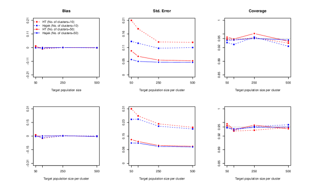
Figure 2: Bias, standard error, and coverage of 95% confidence intervals for the Horvitz-Thompson and Hájek estimators of $\mu^{\pi}_{1}$ under outcome models M1 and M2 and stochastic intervention $\pi^{(1)}_{k}(\cdot)$. The first and second row correspond to outcome models M1 and M2, respectively.

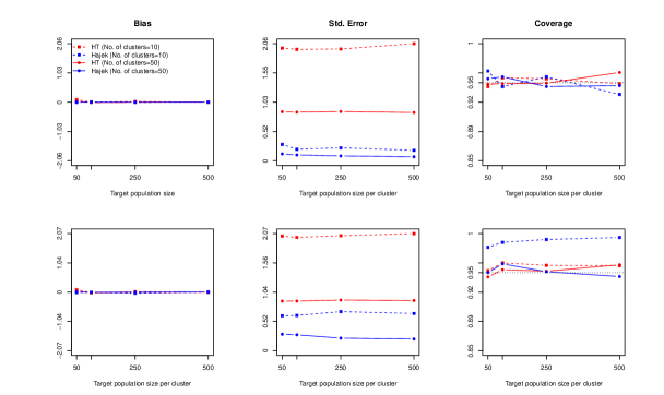
Figure 3: Bias, standard error, and coverage of 95% confidence intervals for the Horvitz-Thompson and Hájek estimators of $\mu^{\pi}_{1}$ under outcome models M1 and M2 and stochastic intervention $\pi^{(2)}_{k}(\cdot)$. The first and second row correspond to outcome models M1 and M2, respectively.

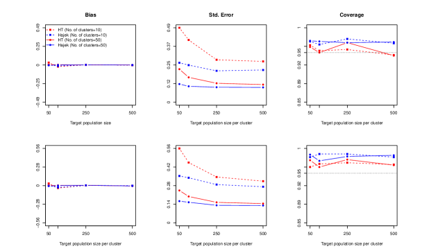
Figure 4: Bias, standard error, and coverage of 95% confidence intervals for the Horvitz-Thompson and Hájek estimators of $\text{DE}^{\pi}$ under outcome models M1 and M2 and stochastic intervention $\pi^{(1)}_{k}(\cdot)$. The first and second row correspond to outcome models M1 and M2, respectively.

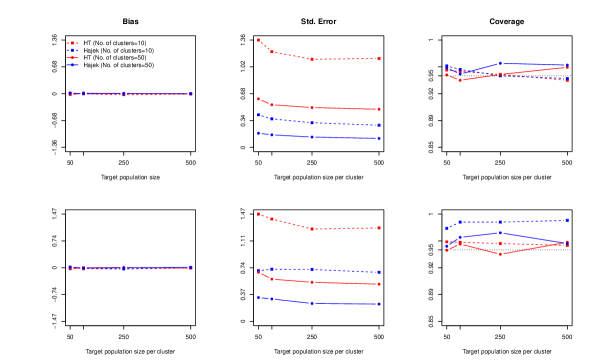
Figure 5: Bias, standard error, and coverage of 95% confidence intervals for the Horvitz-Thompson and Hájek estimators of $\text{DE}^{\pi}$ under outcome models M1 and M2 and stochastic intervention $\pi^{(2)}_{k}(\cdot)$. The first and second row correspond to outcome models M1 and M2, respectively.

6 Empirical application

In this section, we implement our proposed inferential methods using the dataset from the school conflict experiment (Paluck et al. 2016). Our analysis focuses on three outcomes: talking about conflict (yes or no), wearing anti-conflict wristbands (yes or no), and the number of conflict incidents. The first two outcomes serve as indicators of awareness about conflict, while the third outcome quantifies the instances of conflict. The main questions of interest are:

1. On average, what is the effect of each seed-eligible student’s own treatment status on their subsequent conflict behavior?

2. What is the average effect of the treatment status of the best seed-eligible friend of each seed-ineligible student on their subsequent conflict behavior?

3. How do the above effects vary with different proportions of referent students receiving treatment?

4. What is the average effect of treating a fixed proportion (e.g., 0.5) of the close seed-eligible friends of each student on their subsequent conflict behavior?

To address question (i), we define the target population as all seed-eligible students in the network, and for every seed-eligible student $j$, we designate their key-intervention unit as themselves, i.e., $i^{*}(j)=j$. Similarly, to address (ii), we define the target population as all seed-ineligible students in the network, and for every seed-ineligible student $j$, we designate their key-intervention unit as their self-reported closest seed-eligible friend $i^{*}(j)$. In both cases, we set the stochastic intervention $\pi_{k}(\cdot)$ to be equal to the actual intervention $f_{k}(\cdot)$. Table 1 reports the point estimates, standard errors, and 95% confidence intervals for $\mu^{\pi}_{1}$ and $\text{DE}^{\pi}$ under both scenarios.

		Seed-ineligible population			Seed-eligible population
Outcome		Estimate	Std. Error	95% CI	Estimate	Std. Error	95% CI
Talking about conflict	$\hat{\mu}^{\pi}_{1,\text{HT}}$	0.40	0.01	(0.38, 0.43)	0.44	0.01	(0.42, 0.47)
	$\hat{\mu}^{\pi}_{1,\text{H\'{a}jek}}$	0.40	0.01	(0.39, 0.41)	0.44	0.01	(0.42, 0.47)
	$\widehat{\text{DE}}^{\pi}_{\text{HT}}$	0.04	0.02	(-0.01, 0.08)	0.07	0.03	(0.02, 0.12)
	$\widehat{\text{DE}}^{\pi}_{\text{H\'{a}jek}}$	0.02	0.03	(-0.04, 0.07)	0.07	0.03	(0.02, 0.12)
Wearing anti-conflict wristbands	$\hat{\mu}^{\pi}_{1,\text{HT}}$	0.19	0.01	(0.18, 0.21)	0.28	0.01	(0.26, 0.30)
	$\hat{\mu}^{\pi}_{1,\text{H\'{a}jek}}$	0.19	0.01	(0.17, 0.20)	0.28	0.01	(0.26, 0.30)
	$\widehat{\text{DE}}^{\pi}_{\text{HT}}$	0.03	0.01	(-0.002, 0.05)	0.14	0.02	(0.10, 0.18)
	$\widehat{\text{DE}}^{\pi}_{\text{H\'{a}jek}}$	0.02	0.02	(-0.02, 0.05)	0.14	0.02	(0.10, 0.18)
Cases of conflict	$\hat{\mu}^{\pi}_{1,\text{HT}}$	0.16	0.01	(0.14, 0.18)	0.15	0.02	(0.11, 0.18)
	$\hat{\mu}^{\pi}_{1,\text{H\'{a}jek}}$	0.16	0.01	(0.14,0.18)	0.15	0.02	(0.11, 0.18)
	$\widehat{\text{DE}}^{\pi}_{\text{HT}}$	0.00	0.02	(-0.04, 0.05)	0.00	0.03	(-0.07, 0.07)
	$\widehat{\text{DE}}^{\pi}_{\text{H\'{a}jek}}$	-0.01	0.02	(-0.05, 0.04)	0.00	0.03	(-0.07, 0.07)

Table 1: Estimates, standard errors (SE) and $95\%$ confidence intervals (CI) of the average potential outcomes and direct effects for the two target populations, where the stochastic intervention equals the actual intervention.

Table 1 shows that the point estimates and standard errors for the Horvitz-Thompson and Hájek estimators are similar across all scenarios. This finding aligns with those from the simulation study in Section 5, where both the Horvitz Thompson and Hájek estimators performed similarly for large $m_{k}$. When comparing the point estimates of $\mu^{\pi}_{1}$ across the two target populations, we find that under the intervention, the overall level of anti-conflict activities (such as talking about conflict and wearing anti-conflict wristbands) is higher in the seed-eligible population than in the ineligible population. A similar pattern is noted for estimates of $\text{DE}^{\pi}$. These patterns intuitively make sense because the intervention is expected to have a more pronounced effect on students directly involved (i.e., the eligible students) than on their friends who are not eligible. However, this pattern is not as apparent when considering the instances of conflict. Finally, the confidence intervals for $\text{DE}^{\pi}$ indicate that while the intervention on the key-intervention unit increases awareness about conflict (at least among the seed-eligible students), it does not significantly decrease the actual instances of conflict.

Next, we address question (iii) by incorporating information on the referent students in our causal estimands. To this end, for school $k$, we consider a stochastic intervention $\pi_{k}(\cdot)$ that treats a fixed proportion $\alpha$ of referent students (see the Supplementary Materials for details). With varying values of $\alpha$, namely $0.1$, $0.3$, $0.5$, $0.7$, and $0.9$, we plot the corresponding point estimates and 95% confidence intervals for $\mu^{\pi}_{1}$ and $\text{DE}^{\pi}$ in Figures 6 and 7, respectively.

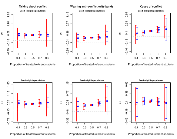
Figure 6: Point estimates and $95\%$ confidence intervals for the Horvitz-Thompson (red) and Hájek (blue) estimators of $\mu^{\pi}_{1}$ for two target populations.

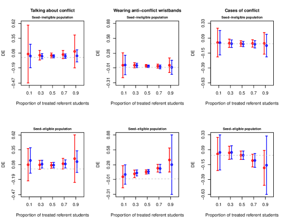
Figure 7: Point estimates and $95\%$ confidence intervals for the Horvitz-Thompson (red) and Hájek (blue) estimators of $\text{DE}^{\pi}$ for two target populations.

Figures 6 and 7 show that the point estimates and standard errors of the Horvitz-Thompson and Hájek estimators exhibit more pronounced differences compared to the previous $\pi_{k}(\cdot)=f_{k}(\cdot)$ scenario. Generally, the Hájek estimator yields smaller standard errors than the Horvitz-Thompson estimator, leading to narrower confidence intervals. The contrast in the overall performance of the estimators for the seed-eligible and ineligible target populations is similar to the previous scenario.

Furthermore, as the proportion of treated referent student $\alpha$ increases, the estimators of $\mu^{\pi}_{1}$ corresponding to conflict awareness (i.e., talking about conflict, wearing wristbands) tend to increase. However, the estimators linked to instances of conflict do not decrease as $\alpha$ increases; in fact, they tend to slightly increase among the seed-ineligible population. Our findings align with those in Paluck et al. (2016), which showed that the peer-to-peer social influence effects of the referent seeds on the instances of conflict are not significant. Also, the confidence intervals for $\text{DE}^{\pi}$ suggest that while in some cases there are significant (positive) direct effects of the intervention on conflict awareness (e.g., on wearing wristbands with $\alpha=0.7$), the effects on instances of conflict are not significant.

Finally, to address question (iv), we define the target population as the set of all students, and for each student $j$, we consider their self-reported close friends (up to 10) as the set of key-intervention units. If $j$ is a seed-eligible student, we include them in the set of key-intervention units. We consider the stochastic intervention as in Section 3.2.3 (see the Supplementary Materials for details). With varying values of $p^{*}$, namely $0.1$, $0.3$, $0.5$, $0.7$, and $0.9$, we depict the corresponding point estimates and 95% confidence intervals for $\tau^{\pi}$ in Figure 8.

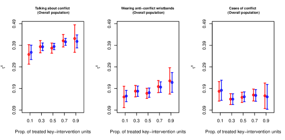
Figure 8: Point estimates and $95\%$ confidence intervals for the Horvitz-Thompson (red) and Hájek (blue) estimators of $\tau^{\pi}$ with multiple key-intervention units.

Figure 8 shows that, similar to the previous cases, the Hájek estimator typically yields narrower confidence intervals for $\tau^{\pi}$ compared to the Horvitz-Thompson estimator. Furthermore, as the proportion of treated close friends increases, the average levels of conflict awareness also tend to increase. The average instances of conflict initially decrease but then plateau as $p^{*}$ is increased from 0.5 to 0.9. In summary, the results suggest that treating a higher proportion of close friends of each student could be beneficial in enhancing awareness about conflict behaviors; however, it may not lead to a reduction in the actual cases of conflict beyond a certain threshold.

7 Concluding remarks

In this paper, we established a design-based framework for the analysis of generalized network experiments, accommodating arbitrary interference and arbitrary target populations. We introduced a class of causal estimands using stochastic interventions and proposed Horvitz-Thompson and Hájek estimators under general interference. We addressed the challenge of identifying the design-based variances of these estimators by developing their conservative estimators.

We implemented the proposed estimation methods in a simulated experiment and a real-world experiment focused on anti-conflict interventions in schools. Both studies suggested that the Hájek estimators tend to produce more precise estimates of causal effects than the Horvitz-Thompson estimators. Our analysis of the school-conflict experiment revealed that intervening on a higher proportion of close friends or referent (i.e., influential) students increases awareness regarding conflict on average, though it does not significantly reduce the average number of conflict cases in schools.

The proposed framework for generalized network experiments can be extended to incorporate more complex estimands and assignment mechanisms. For instance, one could consider treatment assignment mechanisms (both counterfactual and actual) that are dependent across clusters, such as two-stage randomized experiments (Hudgens and Halloran 2008). Potential extensions of this framework include the derivation of large-sample properties of the proposed estimators under weaker assumptions on interference (Sävje et al. 2021).

.

Supplementary Materials

A Proofs of propositions and theorems

A.1 Proof of Theorem 3.1

$${\mathbb{E}}(\hat{\tau}^{\pi}_{\text{HT}}) ={\mathbb{E}}\left[\frac{1}{K}\sum_{k=1}^{K}\left\{\frac{1}{|\mathcal{S}_{k}|}\sum_{j\in\mathcal{S}_{k}}\frac{\pi_{kj}(\bm{A}_{k})}{f_{k}(\bm{A}_{k})}Y^{\text{obs}}_{kj}\right\}\right],$$

$$=\frac{1}{K}\sum_{k=1}^{K}\frac{1}{|\mathcal{S}_{k}|}\sum_{j\in\mathcal{S}_{k}}{\mathbb{E}}\left\{\sum_{\bm{a}}\mathbbm{1}(\bm{A}_{k}=\bm{a})\frac{\pi_{kj}(\bm{a})}{f_{k}(\bm{a})}Y_{kj}(\bm{a})\right\},$$

$$=\frac{1}{K}\sum_{k=1}^{K}\frac{1}{|\mathcal{S}_{k}|}\sum_{j\in\mathcal{S}_{k}}\sum_{\bm{a}}{\mathbb{E}}\{\mathbbm{1}(\bm{A}_{k}=\bm{a})\}\frac{\pi_{kj}(\bm{a})}{f_{k}(\bm{a})}Y_{kj}(\bm{a}),$$

$$=\frac{1}{K}\sum_{k=1}^{K}\frac{1}{|\mathcal{S}_{k}|}\sum_{j\in\mathcal{S}_{k}}\sum_{\bm{a}}f_{k}(\bm{a})\frac{\pi_{kj}(\bm{a})}{f_{k}(\bm{a})}Y_{kj}(\bm{a})$$

$$=\tau^{\pi}.$$

∎

A.2 Proof of Theorem 4.1

The overall variance can be written as,

$${\text{Var}}(\hat{\mu}^{\pi}_{a,\text{HT}})$$

$$= \frac{1}{K^{2}}\sum_{k=1}^{K}\frac{1}{|\mathcal{S}_{k}|^{2}}{\text{Var}}\left(\sum_{j\in\mathcal{S}_{k}}\mathbbm{1}(A_{ki^{*}}=a)\frac{\pi_{k}(\bm{A}_{k(-i^{*})}\mid A_{ki^{*}}=a)}{f_{k}(\bm{A}_{k})}Y^{\text{obs}}_{kj}\right)$$

$$= \frac{1}{K^{2}}\sum_{k=1}^{K}\frac{1}{|\mathcal{S}_{k}|^{2}}{\text{Var}}\left(\sum_{j\in\mathcal{S}_{k}}\sum_{\bm{s}}\mathbbm{1}\{A_{ki^{*}}=a,\bm{A}_{k(-i^{*})}=\bm{s}\}\frac{\pi_{k}(\bm{A}_{k(-i^{*})}=\bm{s}\mid A_{ki^{*}}=a)}{f_{k}(A_{ki^{*}}=a,\bm{A}_{k(-i^{*})}=\bm{s})}Y_{kj}(A_{ki^{*}}=a,\bm{A}_{k(-i^{*})}=\bm{s})\right).$$

The variance term inside the first summation can be decomposed as $\sum_{j\in\mathcal{S}_{k}}\Lambda_{1,kj}+\mathop{\sum\sum}_{j\neq j^{\prime}\in\mathcal{S}_{k}}\Lambda_{2,kj}$, where

$$\Lambda_{1,kj}$$

$$= {\text{Var}}\left\{\sum_{\bm{s}}\mathbbm{1}(A_{ki^{*}}=a,\bm{A}_{k(-i^{*})}=\bm{s})\frac{\pi_{k}(\bm{A}_{k(-i^{*})}=\bm{s}\mid A_{ki^{*}}=a)}{f_{k}(A_{ki^{*}}=a,\bm{A}_{k(-i^{*})}=\bm{s})}Y_{kj}(A_{ki^{*}}=a,\bm{A}_{k(-i^{*})}=\bm{s})\right\}$$

$$= \sum_{\bm{s}}{\text{Var}}\left\{\mathbbm{1}(A_{ki^{*}}=a,\bm{A}_{k(-i^{*})}=\bm{s})\right\}\frac{\pi^{2}_{k}(\bm{A}_{k(-i^{*})}=\bm{s}\mid A_{ki^{*}}=a)}{f^{2}_{k}(A_{ki^{*}}=a,\bm{A}_{k(-i^{*})}=\bm{s})}Y^{2}_{kj}(A_{ki^{*}}=a,\bm{A}_{k(-i^{*})}=\bm{s})$$

$$+\mathop{\sum\sum}_{\bm{s}\neq\bm{s}^{\prime}}{\text{Cov}}\left\{\mathbbm{1}(A_{ki^{*}}=a,\bm{A}_{k(-i^{*})}=\bm{s}),\mathbbm{1}(A_{ki^{*}}=a,\bm{A}_{k(-i^{*})}=\bm{s}^{\prime})\right\}\frac{\pi_{k}(\bm{A}_{k(-i^{*})}=\bm{s}\mid A_{ki^{*}}=a)}{f_{k}(A_{ki^{*}}=a,\bm{A}_{k(-i^{*})}=\bm{s})}$$

$$\hskip 54.2025pt\times\frac{\pi_{k}(\bm{A}_{k(-i^{*})}=\bm{s}^{\prime}\mid A_{ki^{*}}=a)}{f_{k}(A_{ki^{*}}=a,\bm{A}_{k(-i^{*})}=\bm{s}^{\prime})}Y_{kj}(A_{ki^{*}}=a,\bm{A}_{k(-i^{*})}=\bm{s})Y_{kj}(A_{ki^{*}}=a,\bm{A}_{k(-i^{*})}=\bm{s}^{\prime}).$$

$$= \sum_{\bm{s}}\frac{\pi^{2}_{k}(\bm{A}_{k(-i^{*})}=\bm{s}|A_{ki^{*}}=a)\{1-f_{k}(A_{ki^{*}}=a,\bm{A}_{k(-i^{*})}=\bm{s})\}}{f_{k}(A_{ki^{*}}=a,\bm{A}_{k(-i^{*})}=\bm{s})}Y^{2}_{kj}(A_{ki^{*}}=a,\bm{A}_{k(-i^{*})}=\bm{s})$$

$$-\mathop{\sum\sum}_{\bm{s}\neq\bm{s}^{\prime}}\pi_{k}(\bm{A}_{k(-i^{*})}=\bm{s}\mid A_{ki^{*}}=a)\pi_{k}(\bm{A}_{k(-i^{*})}=\bm{s}^{\prime}\mid A_{ki^{*}}=a)$$

$$\hskip 72.26999pt\times Y_{kj}(A_{ki^{*}}=a,\bm{A}_{k(-i^{*})}=\bm{s})Y_{kj}(A_{ki^{*}}=a,\bm{A}_{k(-i^{*})}=\bm{s}^{\prime})$$

$$= \sum_{\bm{s}}\frac{\pi^{2}_{k}(\bm{A}_{k(-i^{*})}=\bm{s}|A_{ki^{*}}=a)}{f_{k}(A_{ki^{*}}=a,\bm{A}_{k(-i^{*})}=\bm{s})}Y^{2}_{kj}(A_{ki^{*}}=a,\bm{A}_{k(-i^{*})}=\bm{s})$$

$$\quad-\left\{\sum_{\bm{s}}\pi_{k}(\bm{A}_{k(-i^{*})}=\bm{s}|A_{ki^{*}}=a)Y_{kj}(A_{ki^{*}}=a,\bm{A}_{k(-i^{*})}=\bm{s})\right\}^{2}$$

and

$$\Lambda_{2,kj}$$

$$= {\text{Cov}}\left(\sum_{\bm{s}}\mathbbm{1}(A_{ki^{*}}=a,\bm{A}_{k(-i^{*})}=\bm{s})\frac{\pi_{k}(\bm{A}_{k(-i^{*})}=\bm{s}\mid A_{ki^{*}}=a)}{f_{k}(A_{ki^{*}}=a,\bm{A}_{k(-i^{*})}=\bm{s})}Y_{kj}(A_{ki^{*}}=a,\bm{A}_{k(-i^{*})}=\bm{s}),\right.$$

$$\hskip 36.135pt\left.\sum_{\bm{s}}\mathbbm{1}(A_{ki^{*^{\prime}}}=a,\bm{A}_{k(-i^{*^{\prime}})}=\bm{s})\frac{\pi_{k}(\bm{A}_{k(-i^{*^{\prime}})}=\bm{s}\mid A_{ki^{*^{\prime}}}=a)}{f_{k}(A_{ki^{*^{\prime}}}=a,\bm{A}_{k(-i^{*^{\prime}})}=\bm{s})}Y_{kj^{\prime}}(A_{ki^{*^{\prime}}}=a,\bm{A}_{k(-i^{*^{\prime}})}=\bm{s})\right),$$

$$= \sum_{\bm{s}}\pi_{k}(\bm{A}_{k(-i^{*})}=\bm{s}\mid A_{ki^{*}}=a)\pi_{k}(\bm{A}_{k(-i^{*^{\prime}})}=\bm{s}\mid A_{ki^{*^{\prime}}}=a)Y_{kj}(A_{ki^{*}}=a,\bm{A}_{k(-i^{*})}=\bm{s})$$

$$\quad\times Y_{kj^{\prime}}(A_{ki^{*^{\prime}}}=a,\bm{A}_{k(-i^{*^{\prime}})}=\bm{s})\left(\frac{\mathbbm{1}\{A_{ki^{*}}=a,A_{ki^{*^{\prime}}}=a,\bm{A}_{k(-i^{*})}=\bm{s},\bm{A}_{k(-i^{*^{\prime}})}=\bm{s}\}}{f_{k}(A_{ki^{*}}=a,\bm{A}_{k(-i^{*})}=\bm{s})}-1\right)$$

$$-\mathop{\sum\sum}_{\bm{s}\neq\bm{s}^{\prime}}\pi_{k}(\bm{A}_{k(-i^{*})}=\bm{s}\mid A_{ki^{*}}=a)\pi_{k}(\bm{A}_{k(-i^{*^{\prime}})}=\bm{s}\mid A_{ki^{*^{\prime}}}=a)$$

$$\hskip 54.2025pt\times Y_{kj}(A_{ki^{*}}=a,\bm{A}_{k(-i^{*})}=\bm{s})Y_{kj^{\prime}}(A_{ki^{*}}=a,\bm{A}_{k(-i^{*^{\prime}})}=\bm{s}^{\prime})$$

$$= \sum_{\bm{s}}\pi_{k}(\bm{A}_{k(-i^{*})}=\bm{s}\mid A_{ki^{*}}=a)\pi_{k}(\bm{A}_{k(-i^{*^{\prime}})}=\bm{s}\mid A_{ki^{*^{\prime}}}=a)Y_{kj}(A_{ki^{*}}=a,\bm{A}_{k(-i^{*})}=\bm{s})$$

$$\quad\times Y_{kj^{\prime}}(A_{ki^{*^{\prime}}}=a,\bm{A}_{k(-i^{*^{\prime}})}=\bm{s})\frac{\mathbbm{1}\{A_{ki^{*}}=a,A_{ki^{*^{\prime}}}=a,\bm{A}_{k(-i^{*})}=\bm{s},\bm{A}_{k(-i^{*^{\prime}})}=\bm{s}\}}{f_{k}(A_{ki^{*}}=a,\bm{A}_{k(-i^{*})}=\bm{s})}$$

$$-\left\{\sum_{\bm{s}}\pi_{k}(\bm{A}_{k(-i^{*})}=\bm{s}\mid A_{ki^{*}}=a)Y_{kj}(A_{ki^{*}}=a,\bm{A}_{k(-i^{*})}=\bm{s})\right\}$$

$$\times\left\{\sum_{\bm{s}}\pi_{k}(\bm{A}_{k(-i^{*^{\prime}})}=\bm{s}\mid A_{ki^{*^{\prime}}}=a)Y_{kj^{\prime}}(A_{ki^{*^{\prime}}}=a,\bm{A}_{k(-i^{*^{\prime}})}=\bm{s})\right\}.$$

∎

A.3 Proof of Proposition 4.2

Without loss of generality, we set $a=1$. The proof for the case of $a=0$ is analogous. Let $\bar{Y}_{kj}(1,\pi_{k})=\sum_{\bm{s}}\pi_{k}(\bm{A}_{k(-i^{*})}=\bm{s}\mid A_{ki^{*}}=1)Y_{kj}(A_{ki^{*}}=1,\bm{A}_{k(-i^{*})}=\bm{s})$. For a completely randomized experiment, $\bar{Y}_{kj}(1,\pi_{k})=\sum_{\bm{s}}Y_{kj}(A_{ki^{*}}=1,\bm{A}_{k(-i^{*})}=\bm{s})/\binom{n_{k}-1}{n_{k1}-1}$. Now, using the notation of Theorem 4.1, we get

$$\Lambda_{1,kj}$$

$$= \frac{1}{\binom{n_{k}}{n_{k1}}p^{2}}\sum_{\bm{s}}Y^{2}_{kj}(A_{ki^{*}}=1,\bm{A}_{k(-i^{*})}=\bm{s})-\bar{Y}^{2}_{kj}(1,\pi_{k})$$

$$= \frac{1}{\binom{n_{k}-1}{n_{k1}-1}}\sum_{\bm{s}}\{Y_{kj}(A_{ki^{*}}=1,\bm{A}_{k(-i^{*})}=\bm{s})-\bar{Y}_{kj}(1,\pi_{k})\}^{2}+\frac{1-p_{k}}{p_{k}\binom{n_{k}-1}{n_{k1}-1}}\sum_{\bm{s}}Y^{2}_{kj}(A_{ki^{*}}=1,\bm{A}_{k(-i^{*})}=\bm{s})$$

$$= \frac{1}{2\binom{n_{k}-1}{n_{k1}-1}^{2}}\mathop{\sum\sum}_{\bm{s}\neq\bm{s}^{\prime}}\{Y_{kj}(A_{ki^{*}}=1,\bm{A}_{k(-i^{*})}=\bm{s})-Y_{kj}(A_{ki^{*}}=1,\bm{A}_{k(-i^{*})}=\bm{s}^{\prime})\}^{2}$$

$$\quad+\frac{1-p_{k}}{p_{k}\binom{n_{k}-1}{n_{k1}-1}}\sum_{\bm{s}}Y^{2}_{kj}(A_{ki^{*}}=1,\bm{A}_{k(-i^{*})}=\bm{s})$$

$$\leq \frac{C(n_{k})^{2}}{2\binom{n_{k}-1}{n_{k1}-1}^{2}}\mathop{\sum\sum}_{\bm{s}\neq\bm{s}^{\prime}}d^{2}(\bm{s},\bm{s}^{\prime})+\frac{1-p_{k}}{p_{k}\binom{n_{k}-1}{n_{k1}-1}}\sum_{\bm{s}}Y^{2}_{kj}(A_{ki^{*}}=1,\bm{A}_{k(-i^{*})}=\bm{s}).$$

The last equality holds since, for $n$ data points $x_{1},....,x_{n}$ with mean $\bar{x}$, $\frac{1}{n}\sum_{i=1}^{n}(x_{i}-\bar{x})^{2}=\frac{1}{2n^{2}}\mathop{\sum\sum}_{i\neq j}(x_{i}-x_{j})^{2}$. The final inequality holds due to the Lipschitz condition. Therefore, we have

$$\sum_{j\in\mathcal{S}_{k}}\Lambda_{1,kj}\leq\frac{C(n_{k})^{2}|\mathcal{S}_{k}|}{2\binom{n_{k}-1}{n_{k1}-1}^{2}}\mathop{\sum\sum}_{\bm{s}\neq\bm{s}^{\prime}}d^{2}(\bm{s},\bm{s}^{\prime})+\frac{1-p_{k}}{p_{k}\binom{n_{k}-1}{n_{k1}-1}}\sum_{j\in\mathcal{S}_{k}}\sum_{\bm{s}}Y^{2}_{kj}(A_{ki^{*}}=1,\bm{A}_{k(-i^{*})}=\bm{s}).$$ (A1)

Next, for two units $j$ and $j^{\prime}$, with key-intervention units $i^{*}$ and $i^{*^{\prime}}$, denote

$$\bar{Y}_{kj}(1,1,\pi_{k})=\frac{1}{\binom{n_{k}-2}{n_{k1}-2}}\sum_{\bm{s}}Y_{kj}(A_{ki^{*}}=1,A_{ki^{*^{\prime}}}=1,\bm{A}_{k(-i^{*},-i^{*^{\prime}})}=\bm{s}).$$

Now,

$$\Lambda_{2,kj}$$

$$= \frac{1}{\binom{n_{k}}{n_{k1}}p^{2}_{k}}\sum_{\bm{s}}Y_{kj}(A_{ki^{*}}=1,A_{ki^{*^{\prime}}}=1,\bm{A}_{k(-i^{*},-i^{*^{\prime}})}=\bm{s})Y_{kj^{\prime}}(A_{ki^{*}}=1,A_{ki^{*^{\prime}}}=1,\bm{A}_{k(-i^{*},-i^{*^{\prime}})}=\bm{s})$$

$$\hskip 50.58878pt-\bar{Y}_{kj}(1,\pi_{k})\bar{Y}_{kj^{\prime}}(1,\pi_{k}).$$

$$= \frac{1}{\binom{n_{k}-2}{n_{k1}-2}}\sum_{\bm{s}}\{Y_{kj}(A_{ki^{*}}=1,A_{ki^{*^{\prime}}}=1,\bm{A}_{k(-i^{*},-i^{*^{\prime}})}=\bm{s})-\bar{Y}_{kj}(1,1,\pi_{k})\}$$

$$\hskip 72.26999pt\times\{Y_{kj^{\prime}}(A_{ki^{*}}=1,A_{ki^{*^{\prime}}}=1,\bm{A}_{k(-i^{*},-i^{*^{\prime}})}=\bm{s})-\bar{Y}_{kj^{\prime}}(1,1,\pi_{k})\}$$

$$\quad+\left(\frac{1}{\binom{n_{k}-1}{n_{k1}-1}p_{k}}-\frac{1}{\binom{n_{k}-2}{n_{k1}-2}}\right)\sum_{\bm{s}}Y_{kj}(A_{ki^{*}}=1,A_{ki^{*^{\prime}}}=1,\bm{A}_{k(-i^{*},-i^{*^{\prime}})}=\bm{s})$$

$$\hskip 72.26999pt\times Y_{kj^{\prime}}(A_{ki^{*}}=1,A_{ki^{*^{\prime}}}=1,\bm{A}_{k(-i^{*},-i^{*^{\prime}})}=\bm{s})$$

$$\quad+\{\bar{Y}_{kj}(1,1,\pi_{k})\bar{Y}_{kj^{\prime}}(1,1,\pi_{k})-\bar{Y}_{kj}(1,\pi_{k})\bar{Y}_{kj^{\prime}}(1,\pi_{k})\}$$ (A2)

Using Cauchy-Schwarz inequality, the first term in Equation (A2) can be upper-bounded as follows,

$$\sum_{\bm{s}}\{Y_{kj}(A_{ki^{*}}=1,A_{ki^{*^{\prime}}}=1,\bm{A}_{k(-i^{*},-i^{*^{\prime}})}=\bm{s})-\bar{Y}_{kj}(1,1,\pi_{k})\}$$

$$\hskip 72.26999pt\times\{Y_{kj^{\prime}}(A_{ki^{*}}=1,A_{ki^{*^{\prime}}}=1,\bm{A}_{k(-i^{*},-i^{*^{\prime}})}=\bm{s})-\bar{Y}_{kj^{\prime}}(1,1,\pi_{k})\}$$

$$\leq\sqrt{\sum_{\bm{s}}\{Y_{kj}(A_{ki^{*}}=1,A_{ki^{*^{\prime}}}=1,\bm{A}_{k(-i^{*},-i^{*^{\prime}})}=\bm{s})-\bar{Y}_{kj}(1,1,\pi_{k})\}^{2}}$$

$$\hskip 72.26999pt\times\sqrt{\sum_{\bm{s}}\{Y_{kj^{\prime}}(A_{ki^{*}}=1,A_{ki^{*^{\prime}}}=1\mid\bm{A}_{k(-i^{*},-i^{*^{\prime}})}=\bm{s})-\bar{Y}_{kj^{\prime}}(1,1,\pi_{k})\}^{2}}$$

$$\leq\frac{C(n_{k})^{2}}{2\binom{n_{k}-2}{n_{k1}-2}}\mathop{\sum\sum}_{\bm{s}\neq\bm{s}^{\prime}}d(\bm{s},\bm{s}^{\prime}),$$

where the last inequality follows from similar steps as in the derivation for $\Lambda_{1,kj}$. Now, suppose that the potential outcomes are bounded by a constant $M$. The third term can be written as,

$$|\bar{Y}_{kj}(1,1,\pi_{k})\bar{Y}_{kj^{\prime}}(1,1,\pi_{k})-\bar{Y}_{kj}(1,\pi_{k})\bar{Y}_{kj^{\prime}}(1,\pi_{k})|$$

$$=\ |\bar{Y}_{kj}(1,1,\pi_{k})\bar{Y}_{kj^{\prime}}(1,1,\pi_{k})-\bar{Y}_{kj}(1,\pi_{k})\bar{Y}_{kj^{\prime}}(1,1,\pi_{k})+\bar{Y}_{kj}(1,\pi_{k})\bar{Y}_{kj^{\prime}}(1,1,\pi_{k})-\bar{Y}_{kj}(1,\pi_{k})\bar{Y}_{kj^{\prime}}(1,\pi_{k})|$$

$$\leq\ M(|\bar{Y}_{kj}(1,1,\pi_{k})-\bar{Y}_{kj}(1,\pi_{k})|+|\bar{Y}_{kj^{\prime}}(1,1,\pi_{k})-\bar{Y}_{kj^{\prime}}(1,\pi_{k})|).$$

Now, $|\bar{Y}_{kj}(1,1,\pi_{k})-\bar{Y}_{kj}(1,\pi_{k})|=\frac{\binom{n_{k}-2}{n_{k1}-1}}{\binom{n_{k}-1}{n_{k1}-1}}|\bar{Y}_{kj}(1,1,\pi_{k})-\bar{Y}_{kj}(1,0,\pi_{k})|\leq\frac{\binom{n_{k}-2}{n_{k1}-1}}{\binom{n_{k}-1}{n_{k1}-1}}C(n_{k})$, which is negligible for sufficiently large $n_{k}$. Therefore, for large $n_{k}$, we can write,

$$\mathop{\sum\sum}_{j\neq j^{\prime}}\Lambda_{2,kj} \leq\frac{|\mathcal{S}_{k}|(|\mathcal{S}_{k}|-1)C(n_{k})^{2}}{2\binom{n_{k}-2}{n_{k1}-2}^{2}}\mathop{\sum\sum}_{\bm{s}\neq\bm{s}^{\prime}}d(\bm{s},\bm{s}^{\prime})$$

$$\quad+\mathop{\sum\sum}_{j\neq j^{\prime}}\left(\frac{1}{\binom{n_{k}-1}{n_{k1}-1}p_{k}}-\frac{1}{\binom{n_{k}-2}{n_{k1}-2}}\right)\sum_{\bm{s}}Y_{kj}(A_{ki^{*}}=1,A_{ki^{*^{\prime}}}=1,\bm{A}_{k(-i^{*},-i^{*^{\prime}})}=\bm{s})$$

$$\hskip 72.26999pt\times Y_{kj^{\prime}}(A_{ki^{*}}=1,A_{ki^{*^{\prime}}}=1,\bm{A}_{k(-i^{*},-i^{*^{\prime}})}=\bm{s}).$$ (A3)

The proof of the proposition follows from Equations (A1) and (A3). ∎

A.4 Proof of Theorem 4.3

Without loss of generality, we set $a=1$. The proof for $a=0$ is analogous. Under Assumptions 5 and 6, $\hat{\mu}^{\pi}_{1,\text{HT}}$ can be written as,

$$\hat{\mu}^{\pi}_{1,\text{HT}} =\frac{1}{K}\sum_{k=1}^{K}\frac{1}{|\mathcal{S}_{k}|}\sum_{j\in\mathcal{S}_{k}}\sum_{\bm{s}:\frac{\bm{s}\top\bm{1}}{n_{k}}=p_{k}}\frac{\mathbbm{1}(A_{ki^{*}}=1,\bm{A}_{k(-i^{*})}=\bm{s})\pi_{k}(\bm{A}_{k(-i^{*})}=\bm{s}\mid A_{ki^{*}}=1)}{f_{k}(A_{ki*}=1,\bm{A}_{k(-i^{*})}=\bm{s})}Y_{kj}(1,p_{k})$$

$$=\frac{1}{K}\sum_{k=1}^{K}\frac{1}{|\mathcal{S}_{k}|}\sum_{i=1}^{n_{k}}\left(\sum_{j\in\mathcal{S}_{k}}\mathbbm{1}(j\leftarrow i)Y_{kj}(1,p_{k})\right)\sum_{\bm{s}}\frac{\mathbbm{1}(A_{ki}=1,\bm{A}_{k(-i)}=\bm{s})\pi_{k}(\bm{A}_{k(-i)}=\bm{s}\mid A_{ki}=1)}{f_{k}(A_{ki}=1,\bm{A}_{k(-i)}=\bm{s})}$$

$$=\frac{1}{K}\sum_{k=1}^{K}\frac{1}{|\mathcal{S}_{k}|}\sum_{i=1}^{n_{k}}\tilde{Y}_{ki}(1,p_{k})\sum_{\bm{s}}\frac{\mathbbm{1}(A_{ki}=1,\bm{A}_{k(-i)}=\bm{s})\pi_{k}(\bm{A}_{k(-i)}=\bm{s}\mid A_{ki}=1)}{f_{k}(A_{ki}=1,\bm{A}_{k(-i)}=\bm{s})}$$

Thus, by Assumption 3,

$${\text{Var}}(\hat{\mu}^{\pi}_{1,\text{HT}})$$

$$=\frac{1}{K^{2}}\sum_{k=1}^{K}\frac{1}{|\mathcal{S}_{k}|^{2}}\left[\sum_{i=1}^{n_{k}}{\text{Var}}\left\{\tilde{Y}_{ki}(1,p_{k})\sum_{\bm{s}}\frac{\mathbbm{1}(A_{ki}=1,\bm{A}_{k(-i)}=\bm{s})\pi_{k}(\bm{A}_{k(-i)}=\bm{s}\mid A_{ki}=1)}{f_{k}(A_{ki}=1,\bm{A}_{k(-i)}=\bm{s})}\right\}\right.$$

$$\quad+\mathop{\sum\sum}_{i\neq i^{\prime}}{\text{Cov}}\left(\tilde{Y}_{ki}(1,p_{k})\sum_{\bm{s}}\frac{\mathbbm{1}(A_{ki}=1,\bm{A}_{k(-i)}=\bm{s})\pi_{k}(\bm{A}_{k(-i)}=\bm{s}\mid A_{ki}=1)}{f_{k}(A_{ki}=1,\bm{A}_{k(-i)}=\bm{s})},\right.$$

$$\hskip 90.3375pt\left.\left.\tilde{Y}_{ki^{\prime}}(1,p_{k})\sum_{\bm{s}}\frac{\mathbbm{1}(A_{ki^{\prime}}=1,\bm{A}_{k(-i^{\prime})}=\bm{s})\pi_{k}(\bm{A}_{k(-i^{\prime})}=\bm{s}\mid A_{ki^{\prime}}=1)}{f_{k}(A_{ki^{\prime}}=1,\bm{A}_{k(-i^{\prime})}=\bm{s})}\right)\right]$$

$$=\frac{1}{K^{2}}\sum_{k=1}^{K}[G_{1k}+G_{2k}],$$

where

$$G_{1k} =\sum_{i=1}^{n_{k}}{\text{Var}}\left(\tilde{Y}_{ki}(1,p_{k})\sum_{\bm{s}}\frac{\mathbbm{1}(A_{ki}=1,\bm{A}_{k(-i)}=\bm{s})\pi_{k}(\bm{A}_{k(-i)}=\bm{s}\mid A_{ki}=1)}{f_{k}(A_{ki}=1,\bm{A}_{k(-i)}=\bm{s})}\right)$$

$$=\sum_{i=1}^{n_{k}}\tilde{Y}^{2}_{ki}(1,p_{k})\left[\sum_{\bm{s}}\frac{{\text{Var}}\{\mathbbm{1}(A_{ki}=1,\bm{A}_{k(-i)}=\bm{s})\}\pi^{2}_{k}(\bm{A}_{k(-i)}=\bm{s}\mid A_{ki}=1)}{f^{2}_{k}(A_{ki}=1,\bm{A}_{k(-i)}=\bm{s})}\right.$$

$$\hskip 108.405pt+\mathop{\sum\sum}_{\bm{s}\neq\bm{s}^{\prime}}{\text{Cov}}\{\mathbbm{1}(A_{ki}=1,\bm{A}_{k(-i)}=\bm{s}),\mathbbm{1}(A_{ki}=1,\bm{A}_{k(-i)}=\bm{s}^{\prime})\}$$

$$\hskip 144.54pt\left.\times\frac{\pi_{k}(\bm{A}_{k(-i)}=\bm{s}\mid A_{ki}=1)\pi_{k}(\bm{A}_{k(-i)}=\bm{s}^{\prime}\mid A_{ki}=1)}{f_{k}(A_{ki}=1,\bm{A}_{k(-i)}=\bm{s})f_{k}(A_{ki}=1,\bm{A}_{k(-i)}=\bm{s}^{\prime})}\right]$$

$$=\sum_{i=1}^{n_{k}}\tilde{Y}^{2}_{ki}(1,p_{k})\left[\sum_{\bm{s}}\pi^{2}_{k}(\bm{A}_{k(-i)}=\bm{s}\mid A_{ki}=1)\frac{1-f_{k}(A_{ki}=1,\bm{A}_{k(-i)}=\bm{s})}{f_{k}(A_{ki}=1,\bm{A}_{k(-i)}=\bm{s})}\right.$$

$$\hskip 108.405pt\left.-\mathop{\sum\sum}_{\bm{s}\neq\bm{s}^{\prime}}\pi_{k}(\bm{A}_{k(-i)}=\bm{s}\mid A_{ki}=1)\pi_{k}(\bm{A}_{k(-i)}=\bm{s}^{\prime}\mid A_{ki}=1)\right]$$

$$=\sum_{i=1}^{n_{k}}c_{i,1}\tilde{Y}^{2}_{ki}(1,p_{k}),$$

$$G_{2k} =\mathop{\sum\sum}_{i\neq i^{\prime}}{\text{Cov}}\left(\tilde{Y}_{ki}(1,p_{k})\sum_{\bm{s}}\frac{\mathbbm{1}(A_{ki}=1,\bm{A}_{k(-i)}=\bm{s})\pi_{k}(\bm{A}_{k(-i)}=\bm{s}\mid A_{ki}=1)}{f_{k}(A_{ki}=1,\bm{A}_{k(-i)}=\bm{s})},\right.$$

$$\hskip 79.49744pt\left.\tilde{Y}_{ki^{\prime}}(1,p_{k})\sum_{\bm{s}}\frac{\mathbbm{1}(A_{ki^{\prime}}=1,\bm{A}_{k(-i^{\prime})}=\bm{s})\pi_{k}(\bm{A}_{k(-i^{\prime})}=\bm{s}\mid A_{ki^{\prime}}=1)}{f_{k}(A_{ki^{\prime}}=1,\bm{A}_{k(-i^{\prime})}=\bm{s})}\right)$$

$$=\mathop{\sum\sum}_{i\neq i^{\prime}}\tilde{Y}_{ki}(1,p_{k})\tilde{Y}_{ki^{\prime}}(1,p_{k})$$

$$\hskip 72.26999pt\times\left[\sum_{\bm{s}}\frac{\pi_{k}(\bm{A}_{k(-i)}=\bm{s}\mid A_{ki}=1)\pi_{k}(\bm{A}_{k(-i^{\prime})}=\bm{s}\mid A_{ki^{\prime}}=1)}{f_{k}(A_{ki}=1,\bm{A}_{k(-i)}=\bm{s})f_{k}(A_{ki^{\prime}}=1,\bm{A}_{k(-i^{\prime})}=\bm{s})}\right.$$

$$\hskip 108.405pt\times{\text{Cov}}\{\mathbbm{1}(A_{ki}=1,\bm{A}_{k(-i)}=\bm{s}),\mathbbm{1}(A_{ki^{\prime}}=1,\bm{A}_{k(-i^{\prime})}=\bm{s})\}$$

$$\hskip 90.3375pt+\mathop{\sum\sum}_{\bm{s}\neq\bm{s}^{\prime}}\frac{\pi_{k}(\bm{A}_{k(-i)}=\bm{s}\mid A_{ki}=1)\pi_{k}(\bm{A}_{k(-i^{\prime})}=\bm{s}^{\prime}\mid A_{ki^{\prime}}=1)}{f_{k}(A_{ki}=1,\bm{A}_{k(-i)}=\bm{s})f_{k}(A_{ki^{\prime}}=1,\bm{A}_{k(-i^{\prime})}=\bm{s}^{\prime})}$$

$$\hskip 108.405pt\times{\text{Cov}}\{\mathbbm{1}(A_{ki}=1,\bm{A}_{k(-i)}=\bm{s}),\mathbbm{1}(A_{ki^{\prime}}=1,\bm{A}_{k(-i^{\prime})}=\bm{s}^{\prime})\}\Big{]}$$

$$=\mathop{\sum\sum}_{i\neq i^{\prime}}\tilde{Y}_{ki}(1,p_{k})\tilde{Y}_{ki^{\prime}}(1,p_{k})\times\frac{1}{\pi_{k}(A_{ki}=1)\pi_{k}(A_{ki^{\prime}}=1)}$$

$$\hskip 72.26999pt\times\left[\sum_{\bm{s}}\frac{\pi_{k}(A_{ki}=1,\bm{A}_{k(-i)}=\bm{s})\pi_{k}(A_{ki^{\prime}}=1,\bm{A}_{k(-i^{\prime})}=\bm{s})}{f_{k}(A_{ki}=1,\bm{A}_{k(-i)}=\bm{s})f_{k}(A_{ki^{\prime}}=1,\bm{A}_{k(-i^{\prime})}=\bm{s})}\right.$$

$$\hskip 108.405pt\times\{f_{k}(A_{ki}=1,\bm{A}_{k(-i)}=\bm{s},A_{ki^{\prime}}=1,\bm{A}_{k(-i^{\prime})}=\bm{s})$$

$$\hskip 108.405pt-f_{k}(A_{ki}=1,\bm{A}_{k(-i)}=\bm{s})f_{k}(A_{ki^{\prime}}=1,\bm{A}_{k(-i^{\prime})}=\bm{s})\}$$

$$\hskip 108.405pt+\mathop{\sum\sum}_{\bm{s}\neq\bm{s}^{\prime}}\frac{\pi_{k}(A_{ki}=1,\bm{A}_{k(-i)}=\bm{s})\pi_{k}(A_{ki^{\prime}}=1,\bm{A}_{k(-i^{\prime})}=\bm{s}^{\prime})}{f_{k}(A_{ki}=1,\bm{A}_{k(-i)}=\bm{s})f_{k}(A_{ki^{\prime}}=1,\bm{A}_{k(-i^{\prime})}=\bm{s}^{\prime})}$$

$$\hskip 144.54pt\times\{-f_{k}(A_{ki}=1,\bm{A}_{k(-i)}=\bm{s})f_{k}(A_{ki^{\prime}}=1,\bm{A}_{k(-i^{\prime})}=\bm{s}^{\prime})\}\Big{]}$$

$$=\mathop{\sum\sum}_{i\neq i^{\prime}}\tilde{Y}_{ki}(1,p_{k})\tilde{Y}_{ki^{\prime}}(1,p_{k})\times\frac{1}{\pi_{k}(A_{ki}=1)\pi_{k}(A_{ki^{\prime}}=1)}$$

$$\quad\times\Big{[}\sum_{\bm{s}}\frac{\pi_{k}(A_{ki}=1,\bm{A}_{k(-i)}=\bm{s})\pi_{k}(A_{ki^{\prime}}=1,\bm{A}_{k(-i)}=\bm{s})}{f_{k}(A_{ki}=1,\bm{A}_{k(-i)}=\bm{s})f_{k}(A_{ki^{\prime}}=1,\bm{A}_{k(-i^{\prime})}=\bm{s})}f_{k}(A_{ki}=1,\bm{A}_{k(-i)}=\bm{s},A_{ki^{\prime}}=1,\bm{A}_{k(-i^{\prime})}=\bm{s})$$

$$\quad-\{\sum_{\bm{s}}\pi_{k}(A_{ki^{\prime}}=1,\bm{A}_{k(-i)}=\bm{s})\}\{\sum_{\bm{s}^{\prime}}\pi_{k}(A_{ki^{\prime}}=1,\bm{A}_{k(-i)}=\bm{s}^{\prime})\}\Big{]}$$

$$=\mathop{\sum\sum}_{i\neq i^{\prime}}d_{ii^{\prime},1}\tilde{Y}_{ki}(1,p_{k})\tilde{Y}_{ki^{\prime}}(1,p_{k}).$$

∎

A.5 Proof of Theorem 4.4

$${\text{Var}}(\widehat{\text{DE}}^{\pi}_{\text{HT}}) ={\text{Var}}(\hat{\mu}^{\pi}_{1,\text{HT}})+{\text{Var}}(\hat{\mu}^{\pi}_{0,\text{HT}})-2{\text{Cov}}(\hat{\mu}^{\pi}_{1,\text{HT}},\hat{\mu}^{\pi}_{0,\text{HT}}).$$

Now, following similar steps as in the proof of Theorem 4.3,

$${\text{Cov}}(\hat{\mu}^{\pi}_{1,\text{HT}},\hat{\mu}^{\pi}_{0,\text{HT}})$$

$$={\text{Cov}}\left(\frac{1}{K}\sum_{k=1}^{K}\frac{1}{|\mathcal{S}_{k}|}\sum_{i=1}^{n_{k}}\frac{\mathbbm{1}(A_{ki}=1)\pi_{k}(\bm{A}_{k(-i)}\mid A_{i}=1)}{f_{k}(\bm{A}_{k})}\tilde{Y}_{ki}(1,p_{k}),\ \frac{1}{K}\sum_{k=1}^{K}\frac{1}{|\mathcal{S}_{k}|}\sum_{i=1}^{n_{k}}\frac{\mathbbm{1}(A_{ki}=0)C}{f_{k}(\bm{A}_{k})}\tilde{Y}_{ki}(0,p_{k})\right)$$

$$=\frac{1}{K^{2}}\sum_{k=1}^{K}\frac{1}{|\mathcal{S}_{k}|^{2}}(G_{k1}+G_{k2}),$$

where

$$G_{1k} =\sum_{i=1}^{n_{k}}\tilde{Y}_{ki}(1,p_{k})\tilde{Y}_{ki}(0,p_{k})\sum_{\bm{s}}\sum_{\bm{s}^{\prime}}\frac{\pi_{k}(\bm{A}_{k(-i)}=\bm{s}\mid A_{ki}=1)\pi_{k}(\bm{A}_{k(-i)}=\bm{s}^{\prime}\mid A_{ki}=0)}{f_{k}(A_{ki}=1,\bm{A}_{k(-i)}=\bm{s})f_{k}(A_{ki}=0,\bm{A}_{k(-i)}=\bm{s}^{\prime})}$$

$$\hskip 144.54pt\times{\text{Cov}}\{\mathbbm{1}(A_{ki}=1,\bm{A}_{k(-i)}=\bm{s}),\mathbbm{1}(A_{ki}=0,\bm{A}_{k(-i)}=\bm{s}^{\prime})\}$$

$$=-\sum_{i=1}^{n_{k}}\tilde{Y}_{ki}(1,p_{k})\tilde{Y}(0,p_{k}),$$

$$G_{2k} =\mathop{\sum\sum}_{i\neq i^{\prime}}\tilde{Y}_{ki}(1,p_{k})\tilde{Y}_{ki^{\prime}}(0,p_{k})\sum_{\bm{s}}\sum_{\bm{s}^{\prime}}\frac{\pi_{k}(\bm{A}_{k(-i)}=\bm{s}\mid A_{ki}=1)\pi_{k}(\bm{A}_{k(-i^{\prime})}=\bm{s}^{\prime}\mid A_{ki^{\prime}}=0)}{f_{k}(A_{ki}=1,\bm{A}_{k(-i)}=\bm{s})f_{k}(A_{ki^{\prime}}=0,\bm{A}_{k(-i^{\prime})}=\bm{s}^{\prime})}$$

$$\hskip 72.26999pt\times{\text{Cov}}\{\mathbbm{1}(A_{ki}=1,\bm{A}_{k(-i)}=\bm{s}),\mathbbm{1}(A_{ki^{\prime}}=0,\bm{A}_{k(-i^{\prime})}=\bm{s}^{\prime})\}$$

$$=\mathop{\sum\sum}_{i\neq i^{\prime}}\frac{\tilde{Y}_{ki}(1,p_{k})\tilde{Y}_{ki^{\prime}}(0,p_{k})}{\pi_{k}(A_{ki}=1)\pi_{k}(A_{ki^{\prime}}=0)}\sum_{\bm{s}}\sum_{\bm{s}^{\prime}}\pi_{k}(A_{ki}=1,\bm{A}_{k(-i)}=\bm{s})\pi_{k}(A_{ki^{\prime}}=0,\bm{A}_{k(-i^{\prime})}=\bm{s}^{\prime})$$

$$\hskip 72.26999pt\times\left\{\frac{f_{k}(A_{ki}=1,\bm{A}_{k(-i)}=\bm{s},A_{ki^{\prime}}=0,\bm{A}_{k(-i^{\prime})}=\bm{s}^{\prime})}{f_{k}(A_{ki}=1,\bm{A}_{k(-i)}=\bm{s})f_{k}(A_{ki^{\prime}}=0,\bm{A}_{k(-i^{\prime})}=\bm{s}^{\prime})}-1\right\}.$$

$$=\mathop{\sum\sum}_{i\neq i^{\prime}}g_{ii^{\prime}}{\tilde{Y}_{ki}(1,p_{k})\tilde{Y}_{ki^{\prime}}(0,p_{k})}$$

∎

A.6 Proof of Proposition 4.5

The variance expressions in (a) and (b) follows from Theorems 4.3 and 4.6 after setting $\pi_{k}(\cdot)=f_{k}(\cdot)$ and $f_{k}(\bm{a})=\mathbbm{1}(\bm{a}^{\top}\bm{1}=n_{k1})/\binom{n_{k}}{n_{k1}}$. Moreover, the unbiasedness and conservativeness of the variance estimators in (a) and (b) follow from the properties of complete randomized design (see, e.g., Imbens and Rubin 2015, Chapter 6).

A.7 Proof of Proposition 4.6

Without loss of generality, we set $a=1$. Following similar steps as in the proof of Theorem 4.3, we get

$${\text{Var}}(\widehat{\text{IE}}^{\pi,\tilde{\pi}}_{1,\text{HT}}) =\frac{1}{K^{2}}\sum_{k=1}^{K}\frac{1}{|\mathcal{S}_{k}|^{2}}{\text{Var}}\left\{\sum_{i=1}^{n_{k}}\sum_{\bm{s}}\gamma_{\bm{s}i}\mathbbm{1}(A_{ki}=1,A_{k(-i)=\bm{s}})\tilde{Y}_{ki}(1,p_{k})\right\},$$

where

$$\gamma_{\bm{s}i} =\frac{\pi_{k}(\bm{A}_{k(-i)}=\bm{s}\mid A_{ki}=1)-\tilde{\pi}_{k}(\bm{A}_{k(-i)}=\bm{s}\mid A_{ki}=1)}{f_{k}(A_{ki}=1,\bm{A}_{k(-i)}=\bm{s})}$$

Therefore,

$${\text{Var}}(\widehat{\text{IE}}^{\pi,\tilde{\pi}}_{1,\text{HT}}) =\frac{1}{K^{2}}\sum_{k=1}^{K}\frac{1}{|\mathcal{S}_{k}|^{2}}(G_{1}+G_{2}),$$

where

$$G_{1} =\sum_{i=1}^{n_{k}}\tilde{Y}^{2}_{ki}(1,p_{k})\Big{[}\sum_{\bm{s]}}\gamma^{2}_{\bm{s}i}f_{k}(A_{ki}=1,\bm{A}_{k(-i)}=\bm{s})\{1-f_{k}(A_{ki}=1,\bm{A}_{k(-i)}=\bm{s})\}$$

$$\quad-\mathop{\sum\sum}_{\bm{s}\neq\bm{s}^{\prime}}\gamma_{\bm{s}i}\gamma_{\bm{s}^{\prime}i}f_{k}(A_{ki}=1,\bm{A}_{k(-i)}=\bm{s})f_{k}(A_{ki}=1,\bm{A}_{k(-i)}=\bm{s}^{\prime})$$

$$=\sum_{i=1}^{n_{k}}\tilde{Y}^{2}_{ki}(1,p_{k})\Big{[}\sum_{\bm{s}}\{\pi_{k}(\bm{A}_{k(-i)}=\bm{s}\mid A_{ki}=1)-\tilde{\pi}_{k}(\bm{A}_{k(-i)}=\bm{s}\mid A_{ki}=1)\}^{2}\frac{\{1-f_{k}(A_{ki}=1,\bm{A}_{k(-i)}=\bm{s})\}}{f_{k}(A_{ki}=1,\bm{A}_{k(-i)}=\bm{s})}$$

$$\quad-\mathop{\sum\sum}_{\bm{s}\neq\bm{s}^{\prime}}\{\pi_{k}(\bm{A}_{k(-i)}=\bm{s}\mid A_{ki}=1)-\tilde{\pi}_{k}(\bm{A}_{k(-i)}=\bm{s}\mid A_{ki}=1)\}$$

$$\hskip 72.26999pt\times\pi_{k}(\bm{A}_{k(-i)}=\bm{s}^{\prime}\mid A_{ki}=1)-\tilde{\pi}_{k}(\bm{A}_{k(-i)}=\bm{s}^{\prime}\mid A_{ki}=1)\}\Big{]}$$

$$=\sum_{i=1}^{n_{k}}\tilde{c}_{i,1}\tilde{Y}^{2}_{ki}(1,p_{k}),$$

$$G_{2} =\mathop{\sum\sum}_{i\neq i^{\prime}}\tilde{Y}_{ki}(1,p_{k})\tilde{Y}_{ki^{\prime}}(1,p_{k})\Big{[}\sum_{\bm{s}}\gamma_{\bm{s}i}\gamma_{\bm{s}i^{\prime}}\{\mathbbm{1}(A_{ki}=1,\bm{A}_{k(-i)}=\bm{s},A_{ki^{\prime}}=1,\bm{A}_{k(-i^{\prime})}=\bm{s})f_{k}(A_{ki}=1,\bm{A}_{k(-i)}=\bm{s})$$

$$\quad-f_{k}(A_{ki}=1,\bm{A}_{k(-i)}=\bm{s})f_{k}(A_{ki^{\prime}}=1,\bm{A}_{k(-i^{\prime})}=\bm{s})\}$$

$$\quad+\mathop{\sum\sum}_{\bm{s}\neq\bm{s}^{\prime}}\gamma_{\bm{s}i}\gamma_{\bm{s}^{\prime}i}\{\mathbbm{1}(A_{ki}=1,\bm{A}_{k(-i)}=\bm{s},A_{ki^{\prime}}=1,\bm{A}_{k(-i^{\prime})}=\bm{s}^{\prime})$$

$$\hskip 72.26999pt\times f_{k}(A_{ki}=1,\bm{A}_{k(-i)}=\bm{s})-f_{k}(A_{ki}=1,\bm{A}_{k(-i)}=\bm{s})f_{k}(A_{ki^{\prime}}=1,\bm{A}_{k(-i^{\prime})}=\bm{s}^{\prime})\}\Big{]}$$

$$=\mathop{\sum\sum}_{i\neq i^{\prime}}\tilde{Y}_{ki}(1,p_{k})\tilde{Y}_{ki^{\prime}}(1,p_{k})\Big{[}\sum_{\bm{s}}\{\pi_{k}(\bm{A}_{k(-i)}=\bm{s}\mid A_{ki}=1)-\tilde{\pi}_{k}(\bm{A}_{k(-i)}=\bm{s}\mid A_{ki}=1)\}$$

$$\hskip 72.26999pt\times\{\pi_{k}(\bm{A}_{k(-i^{\prime})}=\bm{s}\mid A_{ki^{\prime}}=1)-\tilde{\pi}_{k}(\bm{A}_{k(-i^{\prime})}=\bm{s}|A_{ki^{\prime}}=1)\}$$

$$\hskip 72.26999pt\times\Big{\{}\frac{\mathbbm{1}(A_{ki}=1,\bm{A}_{k(-i)}=\bm{s},A_{ki^{\prime}}=1,\bm{A}_{k(-i^{\prime})}=\bm{s})}{f_{k}(A_{ki}=1,\bm{A}_{k(-i)}=\bm{s})}-1\Big{\}}$$

$$\quad-\mathop{\sum\sum}_{\bm{s}\neq\bm{s}^{\prime}}\{\pi_{k}(\bm{A}_{k(-i)}=\bm{s}\mid A_{ki}=1)-\tilde{\pi}_{k}(\bm{A}_{k(-i)}=\bm{s}\mid A_{ki}=1)\}$$

$$\hskip 72.26999pt\times\{\pi_{k}(\bm{A}_{k(-i^{\prime})}=\bm{s}^{\prime}\mid A_{ki^{\prime}}=1)-\tilde{\pi}_{k}(\bm{A}_{k(-i^{\prime})}=\bm{s}^{\prime}\mid A_{ki^{\prime}}=1)\}$$

$$=\mathop{\sum\sum}_{i\neq i^{\prime}}\tilde{d}_{ii^{\prime},1}\tilde{Y}_{ki}(1,p_{k})\tilde{Y}_{ki^{\prime}}(1,p_{k}).$$

∎

A.8 Proof of Theorem 4.7

Without loss of generality, we set $a=1$. Now,

$${\text{Var}}(\hat{\mu}^{\pi}_{1,\text{HT}})=\frac{1}{K^{2}}\sum_{k=1}^{K}\frac{1}{|\mathcal{S}_{k}|^{2}}\left\{\sum_{i=1}^{n_{k}}c_{i,1}\tilde{Y}^{2}_{ki}(1,p_{k})+\mathop{\sum\sum}_{i\neq i^{\prime}}d_{ii^{\prime},1}\tilde{Y}_{ki}(1,p_{k})\tilde{Y}_{ki^{\prime}}(1,p_{k})\right\},$$ (A4)

By the given condition, we have $\hat{\mu}^{\pi}_{1,\text{HT}}-\mu^{\pi}_{1}=O_{P}(1/K)$ and $\hat{\lambda}^{\pi}_{1,\text{HT}}-1=O_{P}(1/K)$ as $K\to\infty$. Therefore, by Slutsky’s theorem, $\hat{\mu}^{\pi}_{1,\text{H\'{a}jek}}=\frac{\hat{\mu}^{\pi}_{1,\text{HT}}}{\hat{\lambda}^{\pi}_{1,\text{HT}}}\xrightarrow{P}\mu^{\pi}_{1}$ as $K\to\infty$. Now, using Taylor’s expansion, for $h(\cdot):\mathbb{R}^{2}\to\mathbb{R}$,

$$h(\hat{\mu}^{\pi}_{1,\text{HT}},\hat{\lambda}^{\pi}_{1,\text{HT}}) =h(\mu^{\pi}_{1},1)+(\hat{\mu}^{\pi}_{1,\text{HT}}-\mu^{\pi}_{1},\hat{\lambda}^{\pi}_{1,\text{HT}}-1)\nabla h(\mu^{\pi}_{1},1)+O_{P}(1/K).$$

Thus, we have

$${\text{Var}}\{h(\hat{\mu}^{\pi}_{1,\text{HT}},\hat{\lambda}^{\pi}_{1,\text{HT}})\}=(\nabla h(\mu^{\pi}_{1},1))^{\top}{\text{Var}}\{(\hat{\mu}^{\pi}_{1,\text{HT}},\hat{\lambda}^{\pi}_{1,\text{HT}})^{\top}\}\nabla h(\mu^{\pi}_{1},1)+o_{P}(1).$$

Setting $h(x,y)=x/y$, we get $\nabla h(x,y)=(1/y,-x/y^{2})$, which implies,

$${\text{Var}}(\hat{\mu}^{\pi}_{1,\text{H\'{a}jek}}) ={\text{Var}}(\hat{\mu}^{\pi}_{1,\text{HT}})+(\mu^{\pi}_{1})^{2}{\text{Var}}(\hat{\lambda}^{\pi}_{1,\text{HT}})-2\mu^{\pi}_{1}{\text{Cov}}(\hat{\mu}^{\pi}_{1,\text{HT}},\hat{\lambda}^{\pi}_{1,\text{HT}})+o_{P}(1).$$

∎

B Additional theoretical results

B.1 Inference on treatment effects with multiple key-intervention units.

In this section, we consider the setting with multiple key-intervention units and focus on the Horvitz-Thompson estimator of $\tau^{\pi}=\frac{1}{K}\sum_{k=1}^{K}\left[\frac{1}{|\mathcal{S}_{k}|}\sum_{j\in\mathcal{S}_{k}}\left\{\sum_{\bm{a}\in\{0,1\}^{n_{k}}}\pi_{k}(\bm{a}|\mathcal{C}_{kj})Y_{kj}(\bm{a})\right\}\right],$ where $\mathcal{C}_{kj}=\{\bm{a}\in\{0,1\}^{n_{k}}:\sum_{s=1}^{r}A_{ki^{*}_{s}}/|\bm{i}^{*}|=p^{*}\}$, where $\bm{i}^{*}$ is the set of key-intervention units of unit $j$ (of size $|\bm{i}^{*}|$), and $p^{*}\in[0,1]$. Here, for each unit $j\in\mathcal{S}_{k}$, the stochastic intervention treats a fixed proportion $p^{*}$ of its key-intervention units. For simplicity, we set $\pi_{k}(\cdot\mid\mathcal{C}_{kj})=f_{k}(\cdot\mid\mathcal{C}_{kj})$, i.e., given that $p^{*}$ proportion of key-intervention units are treated, the assignment mechanism under the stochastic intervention is the same as that under the actual intervention. The resulting Horvitz-Thompson estimator can be written as,

$$\hat{\tau}^{\pi}_{\text{HT}}=\frac{1}{K}\sum_{k=1}^{K}\frac{1}{|\mathcal{S}_{k}|}\sum_{j\in\mathcal{S}_{k}}\frac{\mathbbm{1}(\bm{A}^{\top}_{k\bm{i}^{*}}\bm{1}=|\bm{i}^{*}|p^{*})}{f_{k}(\bm{A}^{\top}_{k\bm{i}^{*}}\bm{1}=|\bm{i}^{*}|p^{*})}Y^{\text{obs}}_{kj}.$$

To point identify the variance of $\hat{\tau}^{\pi}_{\text{HT}}$ in this case, we need an analog of the stratified interference assumption for multiple key-intervention units.

Assumption 7 (Stratified interference for multiple key-intervention units).

For unit $j\in\mathcal{S}_{k}$, if $\bm{a},\bm{a}^{\prime}\in\{0,1\}^{n_{k}}$ are such that $\bm{a}^{\top}_{\bm{i}^{*}}\bm{1}={\bm{a}^{\prime}}^{\top}_{\bm{i}^{*}}\bm{1}$ and $\bm{a}^{\top}\bm{1}=\bm{a}^{\prime\top}\bm{1}$, then $Y_{kj}(\bm{a})=Y_{kj}(\bm{a}^{\prime})$. ∎

Assumption 7 states that the potential outcome of a unit $j\in\mathcal{S}_{k}$ depends on the treatment assignment of the intervention units in cluster $k$ only through the proportion of treated key-intervention units and the proportion of overall treated intervention units. In the single key-intervention unit case, this assumption becomes equivalent to Assumption 5. Under Assumption 7, we can write the potential outcome $Y_{kj}(\bm{a})$ as $Y_{kj}\left(\frac{a^{\top}_{\bm{i}^{*}}\bm{1}}{|\bm{i}^{*}|},\frac{\bm{a}^{\top}\bm{1}}{n_{k}}\right)$.

Similar to the single key-intervention unit case, we now define the pooled potential outcome. However, unlike the previous case, here the pooled potential outcomes are indexed by subsets of the intervention units. Formally, the pooled potential outcome for a subset $\bm{i}$ of $\mathcal{I}_{k}$ and fixed $p^{*},p_{k}\in(0,1)$ is $\tilde{Y}_{k\bm{i}}(p^{*},p_{k})=\sum_{j\in\mathcal{S}_{k}}\mathbbm{1}(j\leftarrow\bm{i})Y_{j}(\frac{a^{\top}_{\bm{i}^{*}}\bm{1}}{|\bm{i}^{*}|}=p^{*},\frac{\bm{a}^{\top}\bm{1}}{n_{k}}=p_{k})$. The corresponding pooled observed outcome is $\tilde{Y}^{\text{obs}}_{k\bm{i}}=\tilde{Y}_{k\bm{i}}(\frac{\bm{A}_{k\bm{i}}^{\top}\bm{1}}{|\bm{i}|},p_{k})$. Also, let $\mathcal{G}_{k}=\{\bm{i}\subseteq\mathcal{I}_{k}:f_{k}(\bm{A}^{\top}_{k\bm{i}}\bm{1}=|\bm{i}|p^{*})>0\}$ be the subset of intervention units $\bm{i}$ in cluster $k$ for which there is a strictly positive probability of observing $p^{*}$ proportion of treated units. In Theorem A1, we obtain a closed-form expression of the variance of $\hat{\tau}^{\pi}_{\text{HT}}$.

Theorem A1.

Under Assumptions 1, 2, 3, 6, 7, and $\pi_{k}(\cdot|\mathcal{C}_{kj})=f_{k}(\cdot|\mathcal{C}_{kj})$,

$${\text{Var}}(\hat{\tau}^{\pi}_{\text{HT}})=\frac{1}{K^{2}}\sum_{k=1}^{K}\frac{1}{|\mathcal{S}_{k}|^{2}}\left[\sum_{\bm{i}\in\mathcal{G}_{k}}\tilde{c}_{\bm{i}}\tilde{Y}^{2}_{k\bm{i}}(p^{*},p_{k})+\mathop{\sum\sum}_{\bm{i}\neq\bm{i}^{\prime}\in\mathcal{G}_{k}}\tilde{d}_{\bm{i}\bm{i}^{\prime}}\tilde{Y}_{k\bm{i}}(p^{*},p_{k})\tilde{Y}_{k\bm{i}^{\prime}}(p^{*},p_{k})\right],$$

where $\tilde{c}_{\bm{i}}=\frac{1}{f_{k}(\bm{A}^{\top}_{k\bm{i}}\bm{1}=|\bm{i}|p^{*})}-1$ and $\tilde{d}_{\bm{i}\bm{i}^{\prime}}=\frac{f_{k}(\bm{A}^{\top}_{k\bm{i}}\bm{1}=|\bm{i}|p^{*},\bm{A}^{\top}_{k\bm{i}^{\prime}}\bm{1}=|\bm{i}|p^{*})}{f_{k}(\bm{A}^{\top}_{k\bm{i}}\bm{1}=|\bm{i}|p^{*})f_{k}(\bm{A}^{\top}_{k\bm{i}^{\prime}}\bm{1}=|\bm{i}^{\prime}|p^{*})}-1$.

The term $\sum_{\bm{i}\in\mathcal{G}_{k}}\tilde{c}_{\bm{i}}\tilde{Y}^{2}_{k\bm{i}}(p^{*},p_{k})$ can be estimated unbiasedly using the Horvitz-Thompson estimator $\sum_{\bm{i}\in\mathcal{G}_{k}}\tilde{c}_{\bm{i}}\frac{\mathbbm{1}(\bm{A}^{\top}_{k\bm{i}}\bm{1}=|\bm{i}|p^{*})}{f_{k}(\bm{A}^{\top}_{k\bm{i}}\bm{1}=|\bm{i}|p^{*})}\tilde{Y}_{k\bm{i}}^{2}$.

Similarly, the Horvitz-Thompson estimator $\mathop{\sum\sum}_{\bm{i}\neq\bm{i}^{\prime}\in\mathcal{G}_{k}}\tilde{d}_{\bm{i}\bm{i}^{\prime}}\frac{\mathbbm{1}(\bm{A}^{\top}_{k\bm{i}}\bm{1}=|\bm{i}|p^{*},\bm{A}^{\top}_{k\bm{i}^{\prime}}\bm{1}=|\bm{i}^{\prime}|p^{*})}{f_{k}(\bm{A}^{\top}_{k\bm{i}}\bm{1}=|\bm{i}|p^{*},\bm{A}^{\top}_{k\bm{i}^{\prime}}\bm{1}=|\bm{i}^{\prime}|p^{*})}\tilde{Y}^{\text{obs}}_{k\bm{i}}\tilde{Y}^{\text{obs}}_{k\bm{i}^{\prime}}$ is unbiased for the term $\mathop{\sum\sum}_{\bm{i}\neq\bm{i}^{\prime}\in\mathcal{G}_{k}}\tilde{d}_{\bm{i}\bm{i}^{\prime}}\tilde{Y}_{k\bm{i}}(p^{*},p_{k})\tilde{Y}_{k\bm{i}^{\prime}}(p^{*},p_{k})$, provided the design satisfies the measurability condition $f_{k}(\bm{A}^{\top}_{k\bm{i}}\bm{1}=|\bm{i}|p^{*},\bm{A}^{\top}_{k\bm{i}^{\prime}}\bm{1}=|\bm{i}^{\prime}|p^{*})>0$, i.e., for all subsets of intervention units $\bm{i},\bm{i}^{\prime}\in\mathcal{G}_{k}$, the design allows for assignments that treat $p^{*}$ proportion of units in both $\bm{i}$ and $\bm{i}^{\prime}$. If the design is not measurable, then we can instead obtain a conservative estimator of the variance. Finally, for some subsets $\bm{i}$, $|\bm{i}|p^{*}$ may not be an integer. In that case, we replace it with its nearest integer $\text{int}(|\bm{i}|p^{*})$. Thus, for a measurable design, we can estimate ${{\text{Var}}}(\hat{\tau^{\pi}_{\text{HT}}})$ as

$$\widehat{{\text{Var}}}(\hat{\tau}^{\pi}_{\text{HT}}) =\frac{1}{K^{2}}\sum_{k=1}^{K}\frac{1}{|\mathcal{S}_{k}|^{2}}\Big{[}\sum_{\bm{i}\in\mathcal{G}_{k}}\tilde{c}_{\bm{i}}\frac{\mathbbm{1}(\bm{A}^{\top}_{k\bm{i}}\bm{1}=\text{int}(|\bm{i}|p^{*}))}{f_{k}(\bm{A}^{\top}_{k\bm{i}}\bm{1}=\text{int}(|\bm{i}|p^{*}))}(\tilde{Y}^{\text{obs}}_{k\bm{i}})^{2}$$

$$\quad+\mathop{\sum\sum}_{\bm{i}\neq\bm{i}^{\prime}\in\mathcal{G}_{k}}\tilde{d}_{\bm{i}\bm{i}^{\prime}}\frac{\mathbbm{1}(\bm{A}^{\top}_{k\bm{i}}\bm{1}=\text{int}(|\bm{i}|p^{*}),\bm{A}^{\top}_{k\bm{i}^{\prime}}\bm{1}=\text{int}(|\bm{i}^{\prime}|p^{*}))}{f_{k}(\bm{A}^{\top}_{k\bm{i}}\bm{1}=\text{int}(|\bm{i}|p^{*}),\bm{A}^{\top}_{k\bm{i}^{\prime}}\bm{1}=\text{int}(|\bm{i}^{\prime}|p^{*}))}\tilde{Y}^{\text{obs}}_{k\bm{i}}\tilde{Y}^{\text{obs}}_{k\bm{i}^{\prime}}\Big{]}.$$

B.2 Proof of Theorem A1

Following the proof of Theorem 4.3, under Assumption 7, we can write

$$\hat{\tau}^{\pi}_{\text{HT}} =\frac{1}{K}\sum_{k=1}^{K}\frac{1}{|\mathcal{S}_{k}|}\sum_{\bm{i}\in\mathcal{G}_{k}}\frac{\mathbbm{1}(\bm{A}^{\top}_{k\bm{i}}\bm{1}=|\bm{i}|p^{*})}{f_{k}(\bm{A}^{\top}_{k\bm{i}}\bm{1}=|\bm{i}|p^{*})}\tilde{Y}_{k\bm{i}}(p^{*},p_{k}).$$

Thus,

$${\text{Var}}(\hat{\tau}^{\pi}_{\text{HT}}) =\frac{1}{K^{2}}\sum_{k=1}^{K}\frac{1}{|\mathcal{S}_{k}|^{2}}\Big{[}\sum_{\bm{i}\in\mathcal{G}_{k}}\frac{1-f_{k}(\bm{A}^{\top}_{k\bm{i}}\bm{1}=|\bm{i}|p^{*})}{f_{k}(\bm{A}^{\top}_{k\bm{i}}\bm{1}=|\bm{i}|p^{*})}\tilde{Y}^{2}_{k\bm{i}}(p^{*},p_{k})$$

$$\quad+\mathop{\sum\sum}_{\bm{i}\neq\bm{i}^{\prime}\in\mathcal{G}_{k}}\tilde{Y}_{k\bm{i}}(p^{*},p_{k})\tilde{Y}_{k\bm{i}^{\prime}}(p^{*},p_{k})\left\{\frac{\Pr(\bm{A}^{\top}_{k\bm{i}}\bm{1}=|\bm{i}|p^{*},\bm{A}^{\top}_{k\bm{i}^{\prime}}\bm{1}=|\bm{i}^{\prime}|p^{*})}{f_{k}(\bm{A}^{\top}_{k\bm{i}}\bm{1}=|\bm{i}|p^{*})f_{k}(\bm{A}^{\top}_{k\bm{i}^{\prime}}\bm{1}=|\bm{i}^{\prime}|p^{*})}-1\right\}\Big{]}$$

$$=\frac{1}{K^{2}}\sum_{k=1}^{K}\frac{1}{|\mathcal{S}_{k}|^{2}}\left[\sum_{\bm{i}\in\mathcal{G}_{k}}\tilde{c}_{\bm{i}}\tilde{Y}^{2}_{k\bm{i}}(p^{*},p_{k})+\mathop{\sum\sum}_{\bm{i}\neq\bm{i}^{\prime}\in\mathcal{G}_{k}}\tilde{d}_{\bm{i}\bm{i}^{\prime}}\tilde{Y}_{k\bm{i}}(p^{*},p_{k})\tilde{Y}_{k\bm{i}^{\prime}}(p^{*},p_{k})\right].$$

∎

B.3 Inference for the Hájek estimator

In Section 4.2, we computed the approximate design-based variance of the Hájek estimator of $\mu^{\pi}_{1}$ and proposed estimators of this variance. Analogously, in this section, we first derive the approximate design-based variance of the Hájek estimator of $\text{DE}^{\pi}$. The Hájek estimator of $\text{DE}^{\pi}$ is given by,

$$\widehat{\text{DE}}^{\pi}_{\text{H\'{a}jek}} =\hat{\mu}^{\pi}_{1,\text{H\'{a}jek}}-\hat{\mu}^{\pi}_{0,\text{H\'{a}jek}}=\frac{\hat{\mu}^{\pi}_{1,\text{HT}}}{\hat{\lambda}^{\pi}_{1,\text{HT}}}-\frac{\hat{\mu}^{\pi}_{0,\text{HT}}}{\hat{\lambda}^{\pi}_{0,\text{HT}}}.$$ (A5)

Under the assumptions of Theorem 4.7, we have, for $a\in\{0,1\}$, $\hat{\mu}^{\pi}_{a,\text{HT}}-\mu^{\pi}_{a}=O_{p}(1/K)$ and $\hat{\lambda}^{\pi}_{a,\text{HT}}-\lambda^{\pi}_{a}=O_{p}(1/K)$. Thus, using Taylor expansion, we get

$${\text{Var}}(h(\hat{\mu}^{\pi}_{0,\text{HT}},\hat{\lambda}^{\pi}_{0,\text{HT}},\hat{\mu}^{\pi}_{1,\text{HT}},\hat{\lambda}^{\pi}_{1,\text{HT}})$$

$$=(\nabla h(\mu^{\pi}_{0},1,\mu^{\pi}_{1},1))^{\top}{\text{Var}}\{(\hat{\mu}^{\pi}_{0,\text{HT}},\hat{\lambda}^{\pi}_{0,\text{HT}},\hat{\mu}^{\pi}_{1,\text{HT}},\hat{\lambda}^{\pi}_{1,\text{HT}})^{\top}\}\nabla h(\mu^{\pi}_{0},1,\mu^{\pi}_{1},1)+o_{P}(1).$$

Now, setting $h(x_{0},y_{0},x_{1},y_{1})=(x_{1}/y_{1})-(x_{0}/y_{0})$, we have $\nabla h(\mu^{\pi}_{0},1,\mu^{\pi}_{1},1)=(-1,\mu^{\pi}_{0},1,-\mu^{\pi}_{1})^{\top}$. Therefore,

$${\text{Var}}(\widehat{\text{DE}}^{\pi}_{\text{H\'{a}jek}}) ={\text{Var}}(\hat{\mu}^{\pi}_{0,\text{HT}})+(\mu^{\pi}_{0})^{2}{\text{Var}}(\hat{\lambda}^{\pi}_{0,\text{HT}})-2\mu^{\pi}_{0}{\text{Cov}}(\hat{\mu}^{\pi}_{0,\text{HT}},\hat{\lambda}^{\pi}_{0,\text{HT}})$$

$$\quad+{\text{Var}}(\hat{\mu}^{\pi}_{1,\text{HT}})+(\mu^{\pi}_{1})^{2}{\text{Var}}(\hat{\lambda}^{\pi}_{1,\text{HT}})-2\mu^{\pi}_{1}{\text{Cov}}(\hat{\mu}^{\pi}_{1,\text{HT}},\hat{\lambda}^{\pi}_{1,\text{HT}})$$

$$\quad-2{\text{Cov}}(\hat{\mu}^{\pi}_{0,\text{HT}},\hat{\mu}^{\pi}_{1,\text{HT}})+2\mu^{\pi}_{1}{\text{Cov}}(\hat{\mu}^{\pi}_{0,\text{HT}},\hat{\lambda}^{\pi}_{1,\text{HT}})+2\mu^{\pi}_{0}{\text{Cov}}(\hat{\lambda}^{\pi}_{0,\text{HT}},\hat{\mu}^{\pi}_{1,\text{HT}})$$

$$\quad-2\mu^{\pi}_{0}\mu^{\pi}_{1}{\text{Cov}}(\hat{\lambda}^{\pi}_{0,\text{HT}},\hat{\lambda}^{\pi}_{1,\text{HT}})+o_{P}(1).$$

Following the proof of Theorem 4.3 and 4.4, we can compute the covariance terms as follows.

$${\text{Cov}}(\hat{\mu}^{\pi}_{a,\text{HT}},\hat{\lambda}^{\pi}_{a,\text{HT}}) =\frac{1}{K^{2}}\sum_{k=1}^{K}\frac{1}{|\mathcal{S}_{k}|^{2}}\Big{\{}\sum_{i=1}^{n_{k}}c_{i,a}\tilde{Y}_{ki}(a,p_{k})D_{ki}+\mathop{\sum\sum}_{i\neq i^{\prime}}d_{ii^{\prime},a}\tilde{Y}_{ki}(a,p_{k})D_{ki^{\prime}}\Big{\}}.$$

$${\text{Cov}}(\hat{\mu}^{\pi}_{1,\text{HT}},\hat{\mu}^{\pi}_{0,\text{HT}}) =\frac{1}{K^{2}}\sum_{k=1}^{K}\frac{1}{|\mathcal{S}_{k}|^{2}}\left[\mathop{\sum\sum}_{i\neq i^{\prime}}g_{ii^{\prime}}\tilde{Y}_{ki}(1,p_{k})\tilde{Y}_{ki^{\prime}}(0,p_{k})-\sum_{i=1}^{n_{k}}\tilde{Y}_{ki}(1,p_{k})\tilde{Y}_{ki}(0,p_{k})\right],$$

$${\text{Cov}}(\hat{\mu}^{\pi}_{1,\text{HT}},\hat{\lambda}^{\pi}_{0,\text{HT}}) =\frac{1}{K^{2}}\sum_{k=1}^{K}\frac{1}{|\mathcal{S}_{k}|^{2}}\left[\mathop{\sum\sum}_{i\neq i^{\prime}}g_{ii^{\prime}}\tilde{Y}_{ki}(1,p_{k})D_{ki^{\prime}}-\sum_{i=1}^{n_{k}}\tilde{Y}_{ki}(1,p_{k})D_{ki}\right],$$

$${\text{Cov}}(\hat{\lambda}^{\pi}_{1,\text{HT}},\hat{\mu}^{\pi}_{0,\text{HT}}) =\frac{1}{K^{2}}\sum_{k=1}^{K}\frac{1}{|\mathcal{S}_{k}|^{2}}\left[\mathop{\sum\sum}_{i\neq i^{\prime}}g_{ii^{\prime}}D_{ki}\tilde{Y}_{ki^{\prime}}(0,p_{k})-\sum_{i=1}^{n_{k}}D_{ki}\tilde{Y}_{ki}(0,p_{k})\right],$$

$${\text{Cov}}(\hat{\lambda}^{\pi}_{1,\text{HT}},\hat{\lambda}^{\pi}_{0,\text{HT}}) =\frac{1}{K^{2}}\sum_{k=1}^{K}\frac{1}{|\mathcal{S}_{k}|^{2}}\left[\mathop{\sum\sum}_{i\neq i^{\prime}}g_{ii^{\prime}}D_{ki}D_{ki^{\prime}}-\sum_{i=1}^{n_{k}}D^{2}_{ki}\right].$$

We estimate the above variance by the plug-in estimator

$$\widehat{{\text{Var}}}(\widehat{\text{DE}}^{\pi}_{\text{H\'{a}jek}}) =\widehat{{\text{Var}}}(\hat{\mu}^{\pi}_{0,\text{HT}})+(\hat{\mu}^{\pi}_{0,\text{H\'{a}jek}})^{2}\widehat{{\text{Var}}}(\hat{\lambda}^{\pi}_{0,\text{HT}})-2\hat{\mu}^{\pi}_{0,\text{H\'{a}jek}}\widehat{{\text{Cov}}}(\hat{\mu}^{\pi}_{0,\text{HT}},\hat{\lambda}^{\pi}_{0,\text{HT}})$$

$$+\widehat{{\text{Var}}}(\hat{\mu}^{\pi}_{1,\text{HT}})+(\hat{\mu}^{\pi}_{1,\text{H\'{a}jek}})^{2}\widehat{{\text{Var}}}(\hat{\lambda}^{\pi}_{1,\text{HT}})-2\hat{\mu}^{\pi}_{1,\text{H\'{a}jek}}\widehat{{\text{Cov}}}(\hat{\mu}^{\pi}_{1,\text{HT}},\hat{\lambda}^{\pi}_{1,\text{HT}})$$

$$-2\widehat{{\text{Cov}}}(\hat{\mu}^{\pi}_{0,\text{HT}},\hat{\mu}^{\pi}_{1,\text{HT}})+2\hat{\mu}^{\pi}_{1,\text{H\'{a}jek}}\widehat{{\text{Cov}}}(\hat{\mu}^{\pi}_{0,\text{HT}},\hat{\lambda}^{\pi}_{1,\text{HT}})+2\hat{\mu}^{\pi}_{0,\text{H\'{a}jek}}\widehat{{\text{Cov}}}(\hat{\lambda}^{\pi}_{0,\text{HT}},\hat{\mu}^{\pi}_{1,\text{HT}})$$

$$-2\hat{\mu}^{\pi}_{0,\text{H\'{a}jek}}\hat{\mu}^{\pi}_{1,\text{H\'{a}jek}}\widehat{{\text{Cov}}}(\hat{\lambda}^{\pi}_{0,\text{HT}},\hat{\lambda}^{\pi}_{1,\text{HT}}).$$

Here, following the proof of Theorem 4.3 and 4.4, we can estimate the covariance terms as,

$$\widehat{{\text{Cov}}}(\hat{\mu}^{\pi}_{a,\text{HT}},\hat{\lambda}^{\pi}_{a,\text{HT}}) =\frac{1}{K^{2}}\sum_{k=1}^{K}\frac{1}{|\mathcal{S}_{k}|^{2}}\Big{\{}\sum_{i=1}^{n_{k}}\frac{\mathbbm{1}(A_{ki}=a)}{f_{k}(A_{ki}=a)}c_{i,a}\tilde{Y}^{\text{obs}}_{ki}D_{ki}+\mathop{\sum\sum}_{i\neq i^{\prime}}\frac{\mathbbm{1}(A_{ki}=a,A_{ki^{\prime}}=a)}{f_{k}(A_{ki}=a,A_{ki^{\prime}}=a)}d_{ii^{\prime},a}\tilde{Y}^{\text{obs}}_{ki}D_{ki^{\prime}}\Big{\}},$$

$$\widehat{{\text{Cov}}}(\hat{\mu}^{\pi}_{1,\text{HT}},\hat{\mu}^{\pi}_{0,\text{HT}}) =\frac{1}{K^{2}}\sum_{k=1}^{K}\frac{1}{|\mathcal{S}_{k}|^{2}}\Big{[}\mathop{\sum\sum}_{i\neq i^{\prime}}g_{ii^{\prime}}\frac{\mathbbm{1}(A_{ki}=1,A_{ki^{\prime}}=0)}{f_{k}(A_{ki}=1,A_{ki^{\prime}}=0)}\tilde{Y}^{\text{obs}}_{ki}\tilde{Y}^{\text{obs}}_{ki^{\prime}}$$

$$-\frac{1}{2}\sum_{i=1}^{n_{k}}\left\{\frac{\mathbbm{1}(A_{ki}=1)}{f_{k}(A_{ki}=1)}+\frac{\mathbbm{1}(A_{ki}=0)}{f_{k}(A_{ki}=0)}\right\}(\tilde{Y}^{\text{obs}}_{ki})^{2}\Big{]},$$

$$\widehat{{\text{Cov}}}(\hat{\mu}^{\pi}_{1,\text{HT}},\hat{\lambda}^{\pi}_{0,\text{HT}}) =\frac{1}{K^{2}}\sum_{k=1}^{K}\frac{1}{|\mathcal{S}_{k}|^{2}}\left[\mathop{\sum\sum}_{i\neq i^{\prime}}g_{ii^{\prime}}\frac{\mathbbm{1}(A_{ki}=1,A_{ki^{\prime}}=0)}{f_{k}(A_{ki}=1,A_{ki^{\prime}}=0)}\tilde{Y}^{\text{obs}}_{ki}D_{ki^{\prime}}-\sum_{i=1}^{n_{k}}\frac{\mathbbm{1}(A_{ki}=1)}{f_{k}(A_{ki}=1)}\tilde{Y}^{\text{obs}}_{ki}D_{ki}\right],$$

$$\widehat{{\text{Cov}}}(\hat{\lambda}^{\pi}_{1,\text{HT}},\hat{\mu}^{\pi}_{0,\text{HT}}) =\frac{1}{K^{2}}\sum_{k=1}^{K}\frac{1}{|\mathcal{S}_{k}|^{2}}\left[\mathop{\sum\sum}_{i\neq i^{\prime}}g_{ii^{\prime}}\frac{\mathbbm{1}(A_{ki}=1,A_{ki^{\prime}}=0)}{f_{k}(A_{ki}=1,A_{ki^{\prime}}=0)}D_{ki}\tilde{Y}^{\text{obs}}_{ki^{\prime}}-\sum_{i=1}^{n_{k}}\frac{\mathbbm{1}(A_{ki}=0)}{f_{k}(A_{ki}=0)}D_{ki}\tilde{Y}^{\text{obs}}_{ki}\right],$$

$$\widehat{{\text{Cov}}}(\hat{\lambda}^{\pi}_{1,\text{HT}},\hat{\lambda}^{\pi}_{0,\text{HT}}) =\frac{1}{K^{2}}\sum_{k=1}^{K}\frac{1}{|\mathcal{S}_{k}|^{2}}\Big{[}\mathop{\sum\sum}_{i\neq i^{\prime}}g_{ii^{\prime}}\frac{\mathbbm{1}(A_{ki}=1,A_{ki^{\prime}}=0)}{f_{k}(A_{ki}=1,A_{ki^{\prime}}=0)}D_{ki}D_{ki^{\prime}}$$

$$-\frac{1}{2}\sum_{i=1}^{n_{k}}\left\{\frac{\mathbbm{1}(A_{ki}=1)}{f_{k}(A_{ki}=1)}+\frac{\mathbbm{1}(A_{ki}=0)}{f_{k}(A_{ki}=0)}\right\}(D_{ki})^{2}\Big{]}.$$

Finally, we conclude the section by considering the multiple key-intervention unit case as in Section B.1. The Hájek estimator of $\tau^{\pi}$ is given by

$$\hat{\tau}^{\pi}_{\text{H\'{a}jek}}=\frac{\sum_{k=1}^{K}\frac{1}{|\mathcal{S}_{k}|}\sum_{j\in\mathcal{S}_{k}}\frac{\mathbbm{1}(\bm{A}^{\top}_{k\bm{i}^{*}}\bm{1}=|\bm{i}^{*}|p^{*})}{f_{k}(\bm{A}^{\top}_{k\bm{i}^{*}}\bm{1}=|\bm{i}^{*}|p^{*})}Y^{\text{obs}}_{kj}}{\sum_{k=1}^{K}\frac{1}{|\mathcal{S}_{k}|}\sum_{j\in\mathcal{S}_{k}}\frac{\mathbbm{1}(\bm{A}^{\top}_{k\bm{i}^{*}}\bm{1}=|\bm{i}^{*}|p^{*})}{f_{k}(\bm{A}^{\top}_{k\bm{i}^{*}}\bm{1}=|\bm{i}^{*}|p^{*})}}=\frac{\hat{\tau}^{\pi}_{\text{HT}}}{\hat{\lambda}^{\pi}_{\text{HT}}}.$$

The form of the variance of $\hat{\tau}^{\pi}_{\text{H\'{a}jek}}$ and its estimator is analogous to those in Theorem 4.7, where $\hat{\mu}^{\pi}_{a,\text{HT}}$ is replaced by $\hat{\tau}^{\pi}_{\text{HT}}$ and $\hat{\lambda}^{\pi}_{a,\text{HT}}$ is replaced by $\hat{\lambda}^{\pi}_{\text{HT}}$, and the derivation is analogous to the proof of Theorem 4.7.

C Additional results from the simulation study

		Model-1								Model-2
	$m_{k}$	Bias		RMSE		Coverage		CI length		Bias		RMSE		Coverage		CI length
		HT	Hájek	HT	Hájek	HT	Hájek	HT	Hájek	HT	Hájek	HT	Hájek	HT	Hájek	HT	Hájek
$K=10$	50	0.01	-0.00	0.21	0.13	0.95	0.94	0.86	0.50	0.01	0.00	0.31	0.25	0.95	0.95	1.23	0.98
	100	-0.01	-0.01	0.18	0.12	0.95	0.93	0.70	0.47	-0.02	-0.02	0.27	0.25	0.94	0.94	1.05	0.96
	250	0.00	0.00	0.13	0.10	0.95	0.95	0.51	0.42	0.00	0.00	0.22	0.21	0.94	0.95	0.86	0.81
	500	-0.00	-0.00	0.13	0.11	0.94	0.93	0.47	0.40	0.00	0.00	0.20	0.19	0.95	0.96	0.79	0.76
$K=50$	50	0.00	-0.00	0.09	0.06	0.95	0.94	0.37	0.23	-0.00	-0.00	0.13	0.11	0.96	0.95	0.52	0.44
	100	0.00	0.00	0.07	0.05	0.95	0.95	0.29	0.21	0.00	0.00	0.12	0.11	0.94	0.94	0.47	0.43
	250	0.00	0.00	0.06	0.05	0.96	0.95	0.23	0.19	0.00	0.00	0.10	0.09	0.95	0.95	0.40	0.37
	500	-0.00	-0.00	0.06	0.05	0.94	0.95	0.21	0.19	-0.01	-0.01	0.10	0.09	0.94	0.95	0.38	0.37

Table A1: Bias, RMSE, coverage and length of $95\%$ confidence intervals for $\mu^{\pi}_{1}$ under stochastic intervention $\pi^{(1)}_{k}(\cdot)$.

		Model-1								Model-2
	$m_{k}$	Bias		RMSE		Coverage		CI length		Bias		RMSE		Coverage		CI length
		HT	Hájek	HT	Hájek	HT	Hájek	HT	Hájek	HT	Hájek	HT	Hájek	HT	Hájek	HT	Hájek
$K=10$	50	0.03	0.00	0.49	0.26	0.96	0.97	2.04	1.15	0.03	0.00	0.56	0.35	0.96	0.98	2.39	1.65
	100	-0.02	-0.01	0.41	0.25	0.95	0.97	1.64	1.07	-0.04	-0.03	0.45	0.34	0.97	0.99	1.98	1.64
	250	0.00	0.00	0.28	0.21	0.96	0.98	1.13	0.96	0.00	0.00	0.34	0.29	0.97	0.99	1.50	1.38
	500	-0.00	-0.00	0.27	0.21	0.94	0.97	1.01	0.93	-0.00	-0.00	0.31	0.27	0.97	0.98	1.35	1.31
$K=50$	50	0.00	-0.00	0.22	0.12	0.96	0.97	0.89	0.53	-0.00	-0.01	0.24	0.16	0.98	0.99	1.03	0.76
	100	0.00	0.00	0.16	0.11	0.95	0.97	0.67	0.47	0.00	0.00	0.20	0.15	0.96	0.97	0.84	0.71
	250	0.00	0.00	0.13	0.10	0.97	0.97	0.52	0.44	0.00	0.01	0.15	0.13	0.98	0.98	0.69	0.62
	500	-0.00	-0.00	0.12	0.10	0.94	0.97	0.45	0.44	-0.01	-0.01	0.14	0.13	0.97	0.99	0.63	0.63

Table A2: Bias, RMSE, coverage and length of $95\%$ confidence intervals for $\text{DE}^{\pi}$ under stochastic intervention $\pi^{(1)}_{k}(\cdot)$.

		Model-1								Model-2
	$m_{k}$	Bias		RMSE		Coverage		CI length		Bias		RMSE		Coverage		CI length
		HT	Hájek	HT	Hájek	HT	Hájek	HT	Hájek	HT	Hájek	HT	Hájek	HT	Hájek	HT	Hájek
$K=10$	50	0.09	-0.00	1.99	0.29	0.94	0.96	7.67	1.05	0.09	-0.01	2.03	0.62	0.95	0.98	7.87	2.28
	100	0.00	0.01	1.96	0.20	0.96	0.94	7.63	0.91	-0.02	-0.01	2.01	0.62	0.96	0.99	7.84	2.31
	250	0.03	-0.01	1.97	0.23	0.95	0.96	7.78	0.90	0.02	-0.04	2.04	0.69	0.96	0.99	8.07	2.47
	500	-0.01	-0.00	2.06	0.18	0.95	0.94	7.83	0.98	-0.00	0.00	2.07	0.66	0.96	0.99	7.88	2.43
$K=50$	50	0.03	0.01	0.86	0.12	0.95	0.95	3.39	0.46	0.03	0.01	0.88	0.29	0.94	0.95	3.46	1.09
	100	-0.01	-0.00	0.86	0.10	0.95	0.96	3.41	0.40	-0.02	-0.01	0.88	0.28	0.95	0.96	3.48	1.09
	250	-0.00	0.00	0.87	0.08	0.95	0.94	3.38	0.32	-0.01	-0.00	0.90	0.22	0.95	0.95	3.50	0.86
	500	0.00	0.00	0.85	0.07	0.96	0.95	3.43	0.27	0.00	0.01	0.89	0.21	0.96	0.94	3.57	0.78

Table A3: Bias, RMSE, coverage and length of $95\%$ confidence intervals for $\mu^{\pi}_{1}$ under stochastic intervention $\pi^{(2)}_{k}(\cdot)$.

		Model-1								Model-2
	$m_{k}$	Bias		RMSE		Coverage		CI length		Bias		RMSE		Coverage		CI length
		HT	Hájek	HT	Hájek	HT	Hájek	HT	Hájek	HT	Hájek	HT	Hájek	HT	Hájek	HT	Hájek
$K=10$	50	0.02	-0.01	1.36	0.41	0.96	0.96	5.33	1.63	0.02	-0.03	1.47	0.70	0.96	0.98	5.79	2.78
	100	-0.00	0.01	1.21	0.36	0.96	0.96	4.74	1.82	-0.03	-0.01	1.41	0.72	0.96	0.99	5.52	2.93
	250	-0.03	-0.00	1.11	0.31	0.95	0.95	4.42	1.77	-0.04	-0.03	1.27	0.71	0.96	0.99	5.01	2.87
	500	-0.01	0.00	1.12	0.28	0.94	0.95	4.26	2.29	-0.01	0.00	1.28	0.67	0.96	0.99	4.90	3.15
$K=50$	50	-0.02	0.02	0.61	0.18	0.95	0.96	2.39	0.72	-0.02	0.02	0.67	0.33	0.95	0.95	2.66	1.29
	100	0.01	-0.00	0.54	0.16	0.94	0.95	2.12	0.64	-0.00	-0.01	0.58	0.31	0.96	0.97	2.32	1.24
	250	0.01	0.00	0.50	0.13	0.95	0.97	1.97	0.54	0.01	-0.00	0.54	0.25	0.94	0.97	2.11	1.03
	500	-0.01	0.00	0.48	0.11	0.96	0.96	1.93	0.48	-0.01	0.01	0.51	0.24	0.96	0.96	2.08	0.95

Table A4: Bias, RMSE, coverage and length of $95\%$ confidence intervals for $\text{DE}^{\pi}$ under stochastic intervention $\pi^{(2)}_{k}(\cdot)$.

References

• Aronow and Samii (2017) Aronow, P. M. and Samii, C. (2017), “Estimating average causal effects under general interference, with application to a social network experiment,” The Annals of Applied Statistics, 11, 1912–1947.
• Athey et al. (2018) Athey, S., Eckles, D., and Imbens, G. W. (2018), “Exact P-values for Network Interference,” Journal of the American Statistical Association, 113, 230–240.
• Baird et al. (2018) Baird, S., Bohren, J. A., McIntosh, C., and Özler, B. (2018), “Optimal design of experiments in the presence of interference,” Review of Economics and Statistics, 100, 844–860.
• Bajari et al. (2023) Bajari, P., Burdick, B., Imbens, G. W., Masoero, L., McQueen, J., Richardson, T. S., and Rosen, I. M. (2023), “Experimental design in marketplaces,” Statistical Science, 1, 1–19.
• Basse and Feller (2018) Basse, G. and Feller, A. (2018), “Analyzing two-stage experiments in the presence of interference,” Journal of the American Statistical Association, 113, 41–55.
• Crépon et al. (2013) Crépon, B., Duflo, E., Gurgand, M., Rathelot, R., and Zamora, P. (2013), “Do labor market policies have displacement effects? Evidence from a clustered randomized experiment,” The quarterly journal of economics, 128, 531–580.
• Díaz and Hejazi (2019) Díaz, I. and Hejazi, N. (2019), “Causal mediation analysis for stochastic interventions,” arXiv preprint arXiv:1901.02776.
• Doudchenko et al. (2020) Doudchenko, N., Zhang, M., Drynkin, E., Airoldi, E., Mirrokni, V., and Pouget-Abadie, J. (2020), “Causal inference with bipartite designs,” arXiv preprint arXiv:2010.02108.
• Fisher (1935) Fisher, R. A. (1935), The design of experiments, London: Oliver & Boyd.
• Fuller (2009) Fuller, W. A. (2009), Sampling statistics, vol. 560, John Wiley & Sons.
• Gupta et al. (2019) Gupta, S., Kohavi, R., Tang, D., Xu, Y., Andersen, R., Bakshy, E., Cardin, N., Chandran, S., Chen, N., Coey, D., et al. (2019), “Top challenges from the first practical online controlled experiments summit,” ACM SIGKDD Explorations Newsletter, 21, 20–35.
• Halloran and Hudgens (2016) Halloran, M. E. and Hudgens, M. G. (2016), “Dependent happenings: a recent methodological review,” Current epidemiology reports, 3, 297–305.
• Halloran and Struchiner (1995) Halloran, M. E. and Struchiner, C. J. (1995), “Causal inference in infectious diseases,” Epidemiology, 142–151.
• Harshaw et al. (2021) Harshaw, C., Sävje, F., Eisenstat, D., Mirrokni, V., and Pouget-Abadie, J. (2021), “Design and analysis of bipartite experiments under a linear exposure-response model,” arXiv preprint arXiv:2103.06392.
• Hudgens and Halloran (2008) Hudgens, M. G. and Halloran, M. E. (2008), “Toward causal inference with interference,” Journal of the American Statistical Association, 103, 832–842.
• Imai et al. (2021) Imai, K., Jiang, Z., and Malani, A. (2021), “Causal inference with interference and noncompliance in two-stage randomized experiments,” Journal of the American Statistical Association, 116, 632–644.
• Imbens and Rubin (2015) Imbens, G. W. and Rubin, D. B. (2015), Causal inference in statistics, social, and biomedical sciences, Cambridge University Press.
• Kennedy (2019) Kennedy, E. H. (2019), “Nonparametric causal effects based on incremental propensity score interventions,” Journal of the American Statistical Association, 114, 645–656.
• Leung (2020) Leung, M. P. (2020), “Treatment and spillover effects under network interference,” Review of Economics and Statistics, 102, 368–380.
• Liu and Hudgens (2014) Liu, L. and Hudgens, M. G. (2014), “Large sample randomization inference of causal effects in the presence of interference,” Journal of the American Statistical Association, 109, 288–301.
• Lohr (2021) Lohr, S. L. (2021), Sampling: design and analysis, CRC press.
• Muñoz and Van Der Laan (2012) Muñoz, I. D. and Van Der Laan, M. (2012), “Population intervention causal effects based on stochastic interventions,” Biometrics, 68, 541–549.
• Neyman (1923, 1990) Neyman, J. (1923, 1990), “On the application of probability theory to agricultural experiments,” Statistical Science, 5, 463–480.
• Nickerson (2008) Nickerson, D. W. (2008), “Is voting contagious? Evidence from two field experiments,” American political Science review, 102, 49–57.
• Paluck et al. (2016) Paluck, E. L., Shepherd, H., and Aronow, P. M. (2016), “Changing climates of conflict: A social network experiment in 56 schools,” Proceedings of the National Academy of Sciences, 113, 566–571.
• Papadogeorgou et al. (2020) Papadogeorgou, G., Imai, K., Lyall, J., and Li, F. (2020), “Causal inference with spatio-temporal data: estimating the effects of airstrikes on insurgent violence in Iraq,” arXiv preprint arXiv:2003.13555.
• Papadogeorgou et al. (2019) Papadogeorgou, G., Mealli, F., and Zigler, C. M. (2019), “Causal inference with interfering units for cluster and population level treatment allocation programs,” Biometrics, 75, 778–787.
• Park and Kang (2022) Park, C. and Kang, H. (2022), “Efficient semiparametric estimation of network treatment effects under partial interference,” Biometrika, 109, 1015–1031.
• Pouget-Abadie et al. (2019) Pouget-Abadie, J., Aydin, K., Schudy, W., Brodersen, K., and Mirrokni, V. (2019), “Variance reduction in bipartite experiments through correlation clustering,” Advances in Neural Information Processing Systems, 32.
• Rosenbaum (2007) Rosenbaum, P. R. (2007), “Interference between units in randomized experiments,” Journal of the American Statistical Association, 102, 191–200.
• Sävje et al. (2021) Sävje, F., Aronow, P., and Hudgens, M. (2021), “Average treatment effects in the presence of unknown interference,” Annals of statistics, 49, 673.
• Sinclair et al. (2012) Sinclair, B., McConnell, M., and Green, D. P. (2012), “Detecting spillover effects: Design and analysis of multilevel experiments,” American Journal of Political Science, 56, 1055–1069.
• Sobel (2006) Sobel, M. E. (2006), “What do randomized studies of housing mobility demonstrate? Causal inference in the face of interference,” Journal of the American Statistical Association, 101, 1398–1407.
• Tchetgen and VanderWeele (2012) Tchetgen, E. J. T. and VanderWeele, T. J. (2012), “On causal inference in the presence of interference,” Statistical methods in medical research, 21, 55–75.
• Toulis and Kao (2013) Toulis, P. and Kao, E. (2013), “Estimation of causal peer influence effects,” in International conference on machine learning, PMLR, pp. 1489–1497.
• Wang (2021) Wang, Y. (2021), “Causal Inference under Temporal and Spatial Interference,” arXiv preprint arXiv:2106.15074.
• Wang et al. (2020) Wang, Y., Samii, C., Chang, H., and Aronow, P. (2020), “Design-based inference for spatial experiments with interference,” arXiv preprint arXiv:2010.13599.
• Young et al. (2014) Young, J. G., Hernán, M. A., and Robins, J. M. (2014), “Identification, estimation and approximation of risk under interventions that depend on the natural value of treatment using observational data,” Epidemiologic methods, 3, 1–19.
• Yu et al. (2022) Yu, C. L., Airoldi, E. M., Borgs, C., and Chayes, J. T. (2022), “Estimating the total treatment effect in randomized experiments with unknown network structure,” Proceedings of the National Academy of Sciences, 119, e2208975119.
• Zhang and Imai (2023) Zhang, Y. and Imai, K. (2023), “Individualized Policy Evaluation and Learning under Clustered Network Interference,” arXiv preprint arXiv:2311.02467.
• Zigler et al. (2020) Zigler, C., Forastiere, L., and Mealli, F. (2020), “Bipartite interference and air pollution transport: Estimating health effects of power plant interventions,” arXiv preprint arXiv:2012.04831.
• Zigler and Papadogeorgou (2021) Zigler, C. M. and Papadogeorgou, G. (2021), “Bipartite causal inference with interference,” Statistical science: a review journal of the Institute of Mathematical Statistics, 36, 109.
.