Entanglement in massive Schwinger model
at finite temperature and density

Abstract

We evaluate the entanglement entropy and entropic function of massive two dimensional QED (Schwinger model) at finite temperature, density, and $\theta$-angle. In the strong coupling regime, the entropic function is dominated by the boson mass for large spatial intervals, and reduces to the CFT result for small spatial intervals. We also discuss the entanglement spectrum at finite temperature and a finite $\theta$-angle.

I Introduction

Quantum entanglement is the central tenet in the quantum description of all physical processes. In essence, quantum many-particle states are superposition states, which remarkably can lead to quantum correlations even when no explicit interaction is present. A quantitative way to capture this correlation is through the entanglement entropy.

Recently, there has been a renewal of interest in many aspects of quantum entanglement ranging from quantum many-body systems to field theory Srednicki (1993); Calabrese and Cardy (2004, 2009); Hastings (2007), with new applications in quantum information science Bauer et al. (2023). Of particular interest is the concept of quantum entanglement flow, and its relation to quantum information flow, storage and encryption Bekenstein (1981).

In nuclear and particle physics, quantum entanglement is inherent, yet the use of the entanglement entropy and its measurement has only started to receive attention recently. The quantum entanglement entropy encoded in the proton-proton (pp) interaction amplitude may be responsible for multiparticle production observed at collider energies Stoffers and Zahed (2013). Also, the quantum entanglement entropy may be directly measurable in both pp and ep collisions at high energies  Stoffers and Zahed (2013); Kharzeev and Levin (2017).

Quantum entanglement in two-dimensional non-conformal gauge theories with fermions has been investigated recently, with particular focus on QED2 Ikeda et al. (2023a) and QCD2 ’t Hooft (1974). QED2 or the Schwinger model Schwinger (1962) has been widely studied also as a testbed for quantum computation Ikeda et al. (2023b); Florio et al. (2023); Ikeda et al. (2021); Klco et al. (2018). It has achieved remarkable notoriety given its solvability (in the massless case), and the non-perturbative aspects of its vacuum structure. Much like QCD4, the vacuum of QED2 exhibits a chiral anomaly, confines by generating a mass gap, exhibits a chiral condensate, theta-vacua and instantons.

In this work, we address the bosonized form of the Schwinger model in matter at a finite $\theta$-angle, in the strong coupling regime. We will use it to address the features of spatial entanglement, with a particular emphasis on the entropic function. We will first discuss the case of cold matter in detail, and then show how to introduce finite temperature.

The organization of the paper is as follows: In section II, we briefly review the bosonized form of QED2 in matter with a finite vacuum $\theta$-angle. The vacuum solutions for different fermion masses and vacuum angles exhibit modulated chiral waves. In section III, we derive the explicit form of the entropic function, which captures the UV-finite part of the spatial entanglement for a single spatial cut. The entropic function is a universal function of the boson mass in QED2 shifted by the temperature and vacuum angle, with no effect from the finite density. It reduces to the known central charge in the CFT limit. In section IV.1, we carry a numerical analysis of the entanglement entropy in QED2 at strong coupling, using the bosonized Hamiltonian. The eigenvalue spectrum of the entangled density matrix, is dominated by a collective eigenmode that is sensitive to the boson mass. Our conclusions are in section V. Some details are given in the appendices.

II Massive QED2 at finite density

The Schwinger model with fermions of mass $m$ at finite chemical potential $\mu$ is defined by Schwinger (1962)

$$S=\int d^{2}x\,\bigg{(}\frac{1}{4}F^{2}_{\mu\nu}+\frac{\theta\tilde{F}}{2\pi}+\overline{\psi}(i\not{D}-m+\mu\gamma^{0})\psi\bigg{)}$$ (1)

with $\not{D}=\not{\partial}-ig\not{A}$. The coupling $g$ has dimension of mass. The extensive interest in QED2 stems from the fact that it bears much in common with two-dimensional QCD (QCD2) and possesses confinement. As a result, the QED2 spectrum involves only chargeless composite excitations. Remarkably, the vacuum state is characterized by a non-trivial chiral condensate, and even topological tunneling configurations much like in QCD2. QED2, unlike QCD2, is exactly solvable in the massless case, a huge advantage in understanding its non-perturbative structure.

Shifting the vacuum angle to the mass term and using the standard bosonization rules recalled in Appendix A, the bosonized form of (1) is readily obtained for small current masses:

$$S=\int d^{2}x\bigg{(}\frac{1}{2}(\partial_{\mu}\phi)^{2}-\frac{1}{2}f^{2}m_{S}^{2}\bigg{(}\frac{\phi}{f}-2{\mu x}\bigg{)}^{2}+f^{2}m_{\pi}^{2}\,{\mathbb{N}}_{g}{\rm cos}\bigg{(}\frac{\phi}{f}-2\mu x-\theta\bigg{)}+\frac{\mu^{2}}{2\pi}\bigg{)}$$ (2)

with the chirally shifted pseudo-scalar mass

$$m_{S}^{2}=\frac{g^{2}}{\pi}\qquad m_{\pi}^{2}=-\frac{m\langle\overline{\psi}\psi\rangle_{0}}{f^{2}}$$ (3)

and manifest periodicity in the vacuum angle. The x-dependent chemical potential in (2) follows from the bosonization rule

$$\frac{1}{2}(\partial_{\mu}\phi)^{2}-2\mu f\partial_{x}\phi=\frac{1}{2}(\partial_{\mu}(\phi+2f\mu x))^{2}+\frac{\mu^{2}}{2\pi}$$

followed by the shift $\phi+2f\mu x\rightarrow\phi$. The origin of $m_{S}$ is anomalous (Schwinger ${\rm U}_{A}$(1) anomaly), and the chiral mass shift $m_{\pi}$ originates from the emergent vacuum chiral condensate. Note that there is no Goldstone mode, owing to the Mermin-Wagner theorem. The shifting of the vacuum angle to the mass term follows from the Fujikawa construction, and dependence on $\theta$ disappears in the chiral limit. The vacuum chiral condensate $\langle\overline{\psi}\psi\rangle_{0}=-\frac{e^{\gamma}}{2\pi}m_{S}$ is fixed using functional techniques (for example, using a torus as a regulator); $\gamma$ is the Euler constant Sachs and Wipf (1992); Steele et al. (1995a). Like in QCD4, the chiral condensate is finite in the chiral limit. In Appendix B, we discuss some subtleties of the chiral condensate on the light front.

The effective potential following from (2) is

$$\mathbb{V}(\phi,\theta,\mu)=$$ (4)

$$\frac{1}{2}m_{S}^{2}\bigg{(}\frac{\phi}{f}-2\mu x\bigg{)}^{2}-m_{\pi}^{2}\,\mathbb{N}_{g}{\rm cos}\bigg{(}\frac{\phi}{f}-2\mu x-\theta\bigg{)}.$$

The vacua are fixed by the minima solutions to the transcendental equation

$${\rm sin}\bigg{(}\frac{\phi_{v}}{f}-2\mu x-\theta\bigg{)}=-\frac{1}{\alpha}\bigg{(}\frac{\phi_{v}}{f}-2\mu x\bigg{)}$$ (5)

with the dimensionless chiral parameter $\alpha=m_{\pi}^{2}/m_{S}^{2}$. The vacua solutions to (5) are shown in Fig. 1. For $\theta=\pi$, the vacuum is doubly degenerate for $\frac{m}{g}>\frac{m*}{g}=1/(2\sqrt{\pi}e^{\gamma})\approx 0.158$, where

$$m^{*}=\frac{m_{S}^{2}}{|\langle\overline{\psi}\psi\rangle_{0}|}.$$

This critical value deduced from a mean field analysis in the strong coupling regime is smaller than the numerical value of approximately $0.33$ reported in Hamer et al. (1982).

For the case $\theta=0$ and $\mu\neq 0$, the vacuum solution is inhomogeneous in space, with $\phi_{v}/f=2\mu x$. The fermion density per length is

$$n_{F}=\langle\psi^{\dagger}\psi(x)\rangle_{\mu}=\frac{1}{\sqrt{\pi}}\partial^{1}\phi_{v}=\frac{\mu}{\pi}\equiv 2\int_{0}^{k_{F}}\frac{dk}{2\pi}$$ (6)

with the Fermi momentum $k_{F}=\mu$ and pressure $P=\frac{k_{F}^{2}}{2\pi}$ as expected. Using the bosonization rules, this inhomogeneous solution gives rise to standing chiral waves in two-dimensions,

$$\langle\overline{\psi}\psi(x)\rangle(\mu,0) = \langle\overline{\psi}\psi\rangle_{0}\,{\rm cos}(\phi_{v}/f)=\langle\overline{\psi}\psi\rangle_{0}\,{\rm cos}(2\mu x),$$

$$\langle\overline{\psi}i\gamma^{5}\psi(x)\rangle(\mu,0) = \langle\overline{\psi}\psi\rangle_{0}\,{\rm sin}(\phi_{v}/f)=\langle\overline{\psi}\psi\rangle_{0}\,{\rm sin}(2\mu x).$$ (7)

The particle-hole (Overhauser) pairing dominates over the particle-particle (BCS) pairing since the Fermi surface is reduced to two disjoint points located $2k_{F}$ apart. This is captured by the oscillations in (II) with wave-number $2k_{F}=2\mu$. The same observations were made for QCD2 Schon and Thies (2000), and QCD4 at strong coupling Park et al. (2000); Rapp et al. (2001).

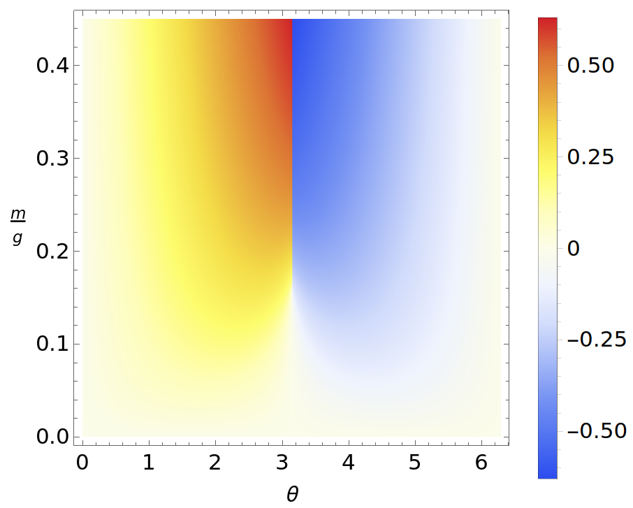
Figure 1: Heatmap of the general vacuum solution $\phi_{v}$ at zero temperature solution to (5). For $\theta=\pi$ and $\frac{m}{g}>0.158$, the vacuum solution is degenerate, with a positive and negative solution. Only the positive solution is shown.

For the case $\theta\neq 0,\pi$, the general vacuum solution follows by shifting away the $x$-dependence $\phi_{v}/f\equiv 2\mu x+\varphi_{v}/f$ in (5), with $\varphi_{v}$ solution to

$${\rm sin}\bigg{(}\frac{\varphi_{v}}{f}-\theta\bigg{)}=-\frac{1}{\alpha}\frac{\varphi_{v}}{f}$$ (8)

For small $\alpha$ near the massless limit,

$$\frac{\varphi_{v}}{f}=\alpha\,{\rm sin}\theta+{\cal O}(\alpha^{2})$$ (9)

with no effect on the fermionic density (6). However, the underlying chiral wave (II) threading the Fermi surface from the Overhauser pairing, is modified

$$\langle\overline{\psi}\psi(x)\rangle(\mu,\theta) \sim \langle\overline{\psi}\psi\rangle_{0}\,{\rm cos}\big{(}2\mu x+\alpha\,{\rm sin}\theta\big{)}$$

$$\langle\overline{\psi}i\gamma^{5}\psi(x)\rangle(\mu,\theta) \sim \langle\overline{\psi}\psi\rangle_{0}\,{\rm sin}\big{(}2\mu x+\alpha\,{\rm sin}\theta\big{)}$$

In general, there are multiple vacua. For $\theta=\pi$ the vacuum is doubly degenerate. The general vacua solutions to (8) for finite $\theta$ are shown in Fig. 1. The sign of the vacuum solution changes around the phase transition line at $\theta=\pi$. In the weak coupling phase with $\frac{m}{g}\gg 1$, the QED2 vacuum breaks C-symmetry or $\varphi_{v}\rightarrow-\varphi_{v}$ symmetry. In the strong coupling phase with $\frac{m}{g}\ll 1$, the QED2 vacuum is C-symmetric with $\varphi_{v}=0$.

III Entropic function

We now consider space to be of length $L$ with a single cut of $l<L$, and study the spatial entanglement of $l$ with $L-l$. The space $L$ can be either periodic (close chain) or open (open chain). For a single cut of length $l$, the spatial entanglement entropy can be analyzed using the replica construction Calabrese and Cardy (2004). The UV insensitive entropic function is given by

$$C(l)=\frac{d{S_{EE}}}{d{\rm ln}l}.$$ (11)

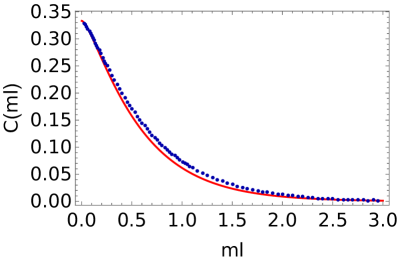
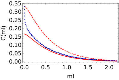
Figure 2: Left: entropic function for a massive fermion for periodic boundary conditions. Right: entropic function for a massive boson for periodic boundary conditions. See text.

III.1 Weak coupling regime: $\frac{m}{g}\gg 1$

In the weak coupling regime, the pseudo-scalar mass is tachyonic, $m_{\theta}^{2}\sim m_{S}^{2}-m_{\pi}^{2}<0$. The normal ordering with respect to the pseudo-scalar mass $m_{S}\ll m$ is no longer justified for heavy fermions. In this regime, we revert to the case of free massive fermions in a screened phase, and use the newly developed field theoretical approach to the entanglement in Liu et al. (2023) using replicated fermions.

In the absence of gauge interactions or screening, the entropic function is given in closed form by that of free massive fermions Liu et al. (2023)

$$C(ml)=\frac{ml}{3}\int_{0}^{1}dx\frac{\,K_{1}\bigg{(}\frac{ml}{\sqrt{x(1-x)}}\bigg{)}}{\sqrt{x(1-x)}}$$ (12)

which is seen to reduce to $C(ml\ll 1)\sim\frac{1}{3}$ in the conformal limit, and asymptote

$$C(ml\gg 1) \sim \sqrt{\frac{\pi ml}{6}}\int_{0}^{1}dx\,\frac{e^{-\frac{ml}{\sqrt{x(1-x)}}}}{(x(1-x))^{\frac{1}{4}}}$$ (13)

$$\sim \sqrt{\frac{\pi ml}{3}}\,e^{-2ml}.$$

(13) is consistent with the asymptotic form derived in Casini and Huerta (2005) using a Painleve V equation for the Renyi entropy, following from the bosonization of free massive fermions and also Goykhman (2015). In Fig. 2 (left) we compare the central charge for the closed chain (12) (solid-red curve) to the exact numerical solution to the Painleve V analysis of the free massive fermion in Casini and Huerta (2005) (dotted-blue curve). The agreement for the fermionic case is remarkable.

In the presence of gauge interactions, the Renyi entropy and the ensuing entropic functions can be organized using standard Feynman graphs with $n$ replicated massive fermions. In the planar approximation, the resummed rainbow diagrams amounts to a shift in the massive free fermion mass for QCD2 Liu et al. (2023).

A rerun of these arguments for QED2 shows that the dressing of the free massive fermion lines with rainbow diagrams yields also a shift

$$m\rightarrow\tilde{m}=\sqrt{m^{2}-m_{S}^{2}}$$ (14)

although the planar approximation is only valid for large replicas in QED2. The ensuing entropic function is still given by (12), but with $m\rightarrow\tilde{m}$. In particular, it reduces to the CFT value of $\frac{1}{3}$ for small intervals. For larger intervals, it asymptotes $e^{-2\tilde{m}l}$ with a range

$$l\approx\frac{1}{2\tilde{m}}<l_{S}\approx\frac{1}{m_{S}}$$

smaller than the screening range at weak coupling, thereby resolving the fermionic structure!

For $m<m_{S}$ the shifted mass is tachyonic, a signal that the weakly interacting phase undergoes a transition to a strongly interacting phase with bound fermions, with a critical value $\frac{m_{*}}{g}=\frac{1}{\sqrt{\pi}}>\frac{1}{\pi}$ in the rainbow approximation.

In general, the effects of temperature in QED2 on a heavy fermion have been analyzed using the invariant fermion propagator in Steele et al. (1995a). For time-like propagation, the bare fermion mass is shifted by the Coulomb self-energy $m\rightarrow m+\frac{\pi m_{S}}{4}$. The temperature correction drops out in the large time limit. For space-like propagation, the fermion is screened with a screening mass $\frac{\pi T}{2}$. We conclude that for a heavy fermion, the result for the entropic function at finite temperature remains (12) after the substitution $m\rightarrow m+\frac{\pi T}{2}$ (space-like cut) and $m\rightarrow m+\frac{\pi m_{S}}{4}$ (time-like cut).

III.2 Strong coupling regime: $\frac{m}{g}\ll 1$

III.2.1 No matter: $\mu=0$, $T=0$

At strong coupling, the vacuum is C-even and the screening is best captured in the bosonized form of QED2. The case of a free massive bosons of mass $m_{B}$ was addressed using the Painleve V analysis, with an entropic function that asymptotes Casini et al. (2005)

$$C(m_{B}l)\sim\frac{m_{B}l}{4}\,K_{1}(2m_{B}l),\qquad m_{B}l\gg 1.$$ (15)

For small intervals, the entropic function converges to the CFT value of $\frac{1}{3}$, in support of the boson-fermion duality in 2-dimensions.

In Fig. 2 (right) we compare the central charge for a closed chain as given by half of (12) (solid-red curve), to the exact numerical solution to the Painleve V analysis for the free massive boson in Casini et al. (2005) (dotted-blue curve). The full-Dirac result (12) (dashed-red curve) is shown for comparison. The overall agreement of the $\frac{1}{2}$-Dirac fermion with the boson is also remarkable, except near the origin, where the massless bosonic fluctuations become dramatically large for small intervals.

A transition between the weak coupling regime with resolved fermions within the screening cloud, and the unresolved screened fermion as a boson in the strong coupling regime, can be differentiated by the entropic function.

III.2.2 Finite density

Using the decomposition $\phi=\phi_{v}+\xi$ around the vacuum solution (5) in the bosonized form (2), we can infer the pertinent bosonic mass for the entropic function. More specifically, the small pseudo-scalar and axion fluctuations of (4) with fixed boundary variations $\delta_{B}\xi=\delta_{B}\vartheta=0$, are coupled both in vacuum and matter,

$$\big{(}\Box+m_{S}^{2}\big{)}\frac{\xi}{f}+m_{\pi}^{2}(T){\rm cos}\bigg{(}\frac{\phi_{v}}{f}+\theta\bigg{)}\bigg{(}\frac{\xi}{f}+\vartheta\bigg{)} = 0,$$

$$\Box\,\vartheta+m_{\pi}^{2}(T){\rm cos}\bigg{(}\frac{\phi_{v}}{f}+\theta\bigg{)}\bigg{(}\frac{\xi}{f}+\vartheta\bigg{)} = 0.$$ (16)

For $\alpha\ll 1$, the pseudo-scalar field carries a squared mass

$$m^{2}_{\theta}\sim m_{S}^{2}+m_{\pi}^{2}{\rm cos}\theta$$ (17)

that is independent of $\mu$. The pseudo-scalar meson disperses relativistically, despite the underlying inhomogeneous chiral wave! The Fermi surface consists only of two points $\pm k_{F}$ in phase space, with minor distortions in the vacuum pairing in the pseudo-scalar channel. This is also manifest from the sizeless light front wavefunction of the pseudo-scalar meson given in appendix B. With this in mind, the asymptotic of the entropic function follows from (15) with $m_{B}\rightarrow m_{\theta}$ or $C(m_{\theta}l)$.

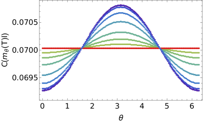
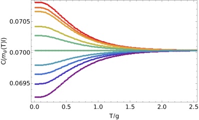
Figure 3: Entropic function in QED2 at strong coupling. Left: as a function of the vacuum angle $\theta$, with increasing temperatures from bottom-purple to top-red; Right: as a function of temperature, with increasing vacuum angle $\theta=\frac{\pi}{20}$ bottom-purple, to $\theta=\pi$ top-red. We have set $m/g=0.0589$ with $l=1$ in units $g=1$.

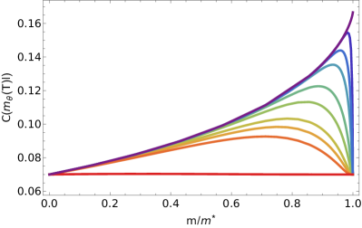
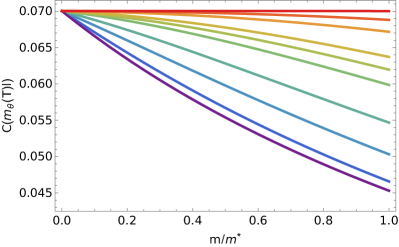
Figure 4: Entropic function versus the current quark mass $\frac{m}{m^{*}}$ for increasing temperatures in the strong coupling phase of QED2: top-purple to bottom-red with $\theta=\pi$ (left), and bottom-purple to top-red with $\theta=0$ (right). The interval length is $l=1$ in units with $g=1$.

III.2.3 Finite temperature

The net effect of the temperature in the massive Schwinger model can be captured by an overall shift of the boson mass through the chiral condensate. Near the massless limit, the boson mass is temperature-dependent, through the chiral condensate

$$m^{2}_{\theta}\rightarrow m_{\theta}^{2}(T)\sim m_{S}^{2}+m_{\pi}^{2}(T){\rm cos}\theta$$ (18)

with the thermal chiral condensate Sachs and Wipf (1992); Smilga (1992); Fayyazuddin et al. (1994); Steele et al. (1995a, b); Durr and Wipf (1997)

$$\langle\overline{\psi}\psi\rangle_{T}=\langle\overline{\psi}\psi\rangle_{0}e^{-2\pi\tilde{\Delta}_{T}(x=0)}$$ (19)

The vacuum-subtracted thermal massive boson propagator is

$$\tilde{\Delta}(x)=\int\frac{d^{2}k}{(2\pi)^{2}}e^{-ikx}\bigg{(}\frac{2\pi\delta(k^{2}-m_{\theta}^{2})}{e^{\frac{|k_{0}|}{T}}-1}\bigg{)}.$$ (20)

Note that (19) can also be regarded as the resummed finite temperature tadpole contribution to the fermionic condensate, stemming from the subsumed normal ordering of the cosine in the bosonized form in (2).

From (19), we conclude that the entropic function for QED2 in dense matter both at finite temperature and density is

$$\frac{lm_{\theta}(T)}{4}\,K_{1}(2lm_{\theta}(T))\qquad lm_{\theta}(T)\gg 1$$ (21)

with the low temperature $T/m_{\theta}\ll 1$ behavior

$$m_{\theta}^{2}(T)\sim m_{S}^{2}+m_{\pi}^{2}{\rm cos}\theta\bigg{(}1-\sqrt{\frac{2\pi T}{m_{\theta}}}e^{-\frac{m_{\theta}}{T}}\bigg{)}$$

and the high temperature $T\gg g^{2}/\pi$ behavior

$$m_{\theta}^{2}(T)\sim m_{S}^{2}-\frac{m}{f^{2}}{\rm cos}\theta\,2Te^{-\frac{\pi T}{m_{\theta}}}.$$ (23)

Note that the chiral condensate has melted.

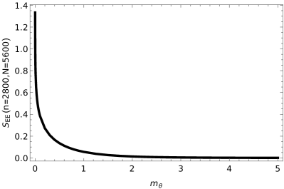
Figure 5: Entanglement entropy for the open chain versus the boson mass $m_{\theta}$ in units of $g=1$.

In Fig. 3 (left) we show the entropic function for a boson as $\frac{1}{2}$-Dirac fermion (12), as a function of the vacuum angle $\theta$, for increasing temperatures from bottom-purple to top-red. The dependence on the vacuum angle disappears at high temperature, following the vanishingly small chiral condensate. The interval size is set to $l=1$ in units where $g=1$, in the strong coupling regime $\frac{m}{g}=0.0589$. The high temperature limit $C(m_{S}l)\sim 0.070$ corresponds to a ’large interval’ as per the right panel of Fig. 2. Fig. 3 (right) is an enlargement in the high temperature limit, where the dependence on the vacuum angle disappears following the vanishing of the vacuum chiral condensate at high temperature. For $\theta=\frac{\pi}{2},\frac{3\pi}{2}$, there is no dependence on the vacuum angle, as the thermal chiral condensate drops out (the ’pion mass’ contribution vanishes).

In the right panel of Fig. 3 we show the same entropic function versus temperature, with the vacuum angle increasing from $\theta=\frac{\pi}{20}$ (bottom-purple) to $\theta=\pi$ (top-red). For $\theta=\frac{\pi}{2}$ the entropic function is independent of the temperature since the vacuum chiral condensate vanishes.

In Fig. 4 we show again the entropic function versus the current quark mass $\frac{m}{m^{*}}$ with fixed vacuum angle $\theta=\pi$ (left) and $\theta=0$ (right), for increasing temperatures from $T=0$ (upper-purple) to high temperature (bottom-red). The critical mass $m^{*}$ is set by the tachyon condition or vanishing of the $\eta^{\prime}$ mass at $\theta=\pi$

$$m_{S}^{2}+m^{*}|\langle\overline{\psi}\psi\rangle|{\rm cos}\pi=0.$$

At $\theta=0$, the entropic function dependence on the current mass ratio $\frac{m}{m^{*}}$ drops out as the ’pion mass’ vanishes exponentially. At $\theta=\pi$ and zero temperature, the entropic function reaches the CFT limit of $\frac{1}{6}$ at $m=m^{*}$. With increasing temperature, the CFT limit is never reached at $m=m^{*}$, which is a high temperature point whatever $T$ since the pseudoscalar mass $m_{\theta}$ ($\eta^{\prime}$ mass) vanishes. The entanglement entropy is maximal at the quantum critical point with $\theta=\pi$ and $\frac{m_{*}}{g}$ as shown in Fig. 5 (CFT point with a massless boson), as noted initially in Ikeda et al. (2023a).

IV Entanglement density matrix at finite temperature

The entropic function indicates that in the regime of large $lm_{\theta}\gg 1$, massive QED2 in matter behaves like that of a free massive boson, while in the regime of small $lm_{\theta}\ll 1$, it resembles a CFT. To characterize the spectral properties of the entangled density it is then sufficient to analyze the quadratic Hamiltonian from bosonized QED2.

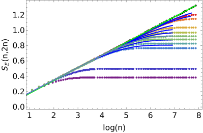
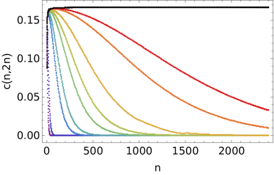
Figure 6: Left: entanglement entropy $S_{E}(n,N=2n)$ for the open chain with different masses; Right: central charge for different masses, with the massless CFT limit $\frac{1}{6}$ shown in solid-black. See text.

IV.1 Chain Hamiltonian

The small fluctuation Hamiltonian following from (4) is given by

$$\mathbb{H}=\int dx\frac{1}{2}\big{(}\Pi^{2}+{\xi^{\prime 2}}+{m_{\theta}^{2}(T)}\xi^{2}\big{)}.$$ (24)

The boson mass is temperature and vacuum angle dependent from QED2. The discretized form of (24) is

$$\mathbb{H}\rightarrow\frac{1}{2}\sum_{i=1}^{N}\big{(}\Pi_{i}^{2}+(\xi_{i+1}-\xi_{i})^{2}+a^{2}m_{\theta}^{2}(T)\xi_{i}^{2}\big{)}$$ (25)

with the chain spacing $a$ for large $l=na\,,L=Na$ but fixed ratio $l/L$. (25) describes a discrete chain of coupled oscillators with nearest neighbor couplings, with either open ($\xi_{N+1}=\xi_{1}=0$) or closed ($\xi_{N+1}=\xi_{1}$) boundary conditions. (25) can be recast as

$$\frac{1}{2}\sum_{i=1}^{N}\Pi_{i}^{2}+\frac{1}{2}\sum^{N}_{i,j=1}\xi_{i}\mathbb{K}_{ij}\xi_{j}$$ (26)

with the real, symmetric and banded matrix

$$\mathbb{K}_{ij}=(2+a^{2}m_{\theta}^{2}(T))\delta_{ij}-\delta_{i,j+1}-\delta_{i,j-1}.$$ (27)

The ground state of the chain (25-26) is

$$\Psi[\xi]=\bigg{(}\frac{|{\Omega}|}{\pi^{N}}\bigg{)}^{\frac{1}{4}}e^{-\frac{1}{2}\sum_{i,j=1}^{N}\xi_{i}\Omega_{ij}\xi_{j}}$$ (28)

with energy $E=\frac{1}{2}{\rm Tr}\,\Omega$. The covariance matrix $\Omega$ can be regarded as the square root of $\mathbb{K}$ under orthogonal rotations. The details of the diagonalization of $\Omega$ are given in Appendix C.

$m_{\theta}$ (eq. (24))	Parameters eq. (62)
	$m^{c}_{\theta}$	shift $\Lambda^{\prime}$
$7\cdot 10^{-4}$	0.00020	0.013
$10^{-3}$	0.00031	0.014
$2\cdot 10^{-3}$	0.00063	0.015
$3\cdot 10^{-3}$	0.001	0.0165
$4\cdot 10^{-3}$	0.00139	0.0174
$5\cdot 10^{-3}$	0.00175	0.0185
$7\cdot 10^{-3}$	0.00245	0.019
$10^{-2}$	0.0037	0.021

Table 1: Relation of mass (24) used in numerics to continuum formula (62) in units of $a=1$.

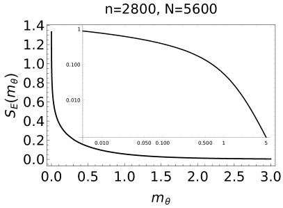
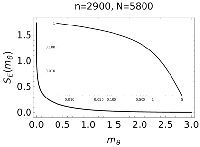
Figure 7: Left: EE for an open chain of size $n$ versus $m_{\theta}$. Right: EE for a closed chain of size $n$ versus $m_{\theta}$. Both insets are double logarithmic plots.

IV.2 Entanglement density matrix

The pure density matrix of the ground state of the open chain is given by

$$\rho[\xi,\xi^{\prime}]=\Psi[\xi]\Psi^{T}[\xi^{\prime}].$$ (29)

The entanglement density matrix can be obtained by subdividing the chain $[\xi]\rightarrow[\underline{\xi},\bar{\xi}]$

$$\rho_{E}[\bar{\xi},{\bar{\xi}}^{\prime}]=\sum_{\underline{\xi}}\Psi[\underline{\xi},{\bar{\xi}}]\Psi^{T}[\underline{\xi},{\bar{x}}^{\prime}].$$ (30)

The positive eigenvalues follow by diagonalizing (30)

$$\sum_{{\bar{\xi}}^{\prime}}\rho_{E}[\bar{\xi},{\bar{\xi}}^{\prime}]\psi_{l}[{\bar{\xi}}^{\prime}]=p_{l}\psi_{l}[\bar{\xi}]$$ (31)

with the entanglement entropy

$$S_{E}=-\sum_{l=0}^{\infty}p_{l}\,{\rm ln}\,p_{l}.$$ (32)

The implicit form of $p_{l}$ from the blocking of the covariance matrix $\Omega$ for the open and closed chains are given in Appendix C.

IV.3 Entanglement Spectrum

We consider the Gram–Schmidt orthonormalization of the ground state

$$\Psi[\xi]=\sum_{i=1}c_{i}\Psi^{A}_{i}[\xi]\Psi^{B}_{i}[\xi],$$ (33)

where $A$ and $B$ denote the non-empty disjoint subspaces such that $A\cup B=\{1,\cdots,N\}$. The entanglement spectrum is defined by the set of the coefficients $\{c_{i}\}$. In our previous paper Ikeda et al. (2023a), we showed numerically that the gaps in the entanglement spectrum close around the critical point.

IV.4 Numerical results

For the blocked chain Hamiltonian, the explicit eigenvalues are given by (57), hence

$$S_{E}(n,N)=-\sum_{i=1}^{n}\sum_{l=0}^{\infty}p_{l}[N,n,i]\,{\rm ln}\,p_{l}[N,n,i]=-\sum_{i=1}^{n}\bigg{(}{\rm ln}(1-\lambda_{N,n,i})+\frac{\lambda_{N,n,i}}{1-\lambda_{N,n,i}}\,{\rm ln}\,\lambda_{N,n,i}\bigg{)}$$ (34)

In Fig. 6-left, we show the entanglement entropy results for the massless and open chain in $m_{\theta}=0$ (black). The green dashed line is (62) with $m_{\theta}\to 0$ shifted by $+0.01(1)$. The curve can also be fitted with

$$0.0108+0.1666\log(n)$$

with the slope converging to the continuum limit of $\frac{1}{6}$.

The rainbow colored lines are for a massive open chain with fixed $a=1$ and increasing masses $m_{\theta}=\{7\cdot 10^{-4},10^{-3},2\cdot 10^{-3},3\cdot 10^{-3},4\cdot 10^{-3},5\cdot 10^{-3},7\cdot 10^{-3},10^{-2},5\cdot 10^{-2},10^{-1}\}$ (rainbow from red-top to purple-bottom). They may be fitted by the continuum result (62) by choosing the parameters indicated in table 1. The masses are approximately related by $m^{c}_{\theta}\sim m_{\theta}^{1.2}$ and the shift scales approximately like $0.0044\log(12.20+9810\,m_{\theta})$.

In Fig. 6-right, we show the numerical results for the corresponding central charge versus the interval length $na\equiv n$ for the open chain at different temperatures, following from Fig. 6 (left) according to Eq. (11) (the color coding of the curves corresponding to varying the mass is identical to Fig. 6-left). For small intervals, the central charge is $\frac{1}{6}$ as expected from CFT, whatever the temperature. For large intervals, the central charges is seen to increase from low temperature (solid-purple) to high temperature (solid-red) as the $\eta^{\prime}$ mass becomes lighter. The black-solid curve is the CFT limit.

In Figs. 7, we show the EE for an open chain (left) and a closed chain (right) with fixed interval size $n$, in QED2 at strong coupling, as a function of the mass $m_{\theta}$. The inset is a double logarithmic plot. The large logarithmic enhancement at small $m_{\theta}$, reflects on the CFT limit. In the large mass limit, the fall off is exponential.

V Conclusions

We have used the bosonized form of QED2 with a finite vacuum angle, to understand quantitatively the nature and aspects of quantum entanglement in space. At weak coupling the QED2 vacuum breaks C-symmetry and chiral symmetry, with C-symmetry restored at strong coupling.

When matter is added, a spatially inhomogeneous chiral density wave threading the Fermi-surface by Overhauser (particle-hole) pairing forms. The chiral condensate is depleted by thermal effects. The massive boson of the interacting theory carries a thermal mass that is only sensitive to the chiral condensate.

To quantify the spatial entanglement in QED2, we have traced out a spatial interval. The spatial entanglement entropy is a function of the length of this spatial interval, the temperature and the vacuum angle. For fixed temperature, the central charge increases with vacuum angle. At high temperature, the central charge is insensitive to the vacuum angle, as the chiral condensate becomes exponentially suppressed.

To check our mean field results numerically in the strong coupling regime, we have made use of the bosonized Hamiltonian for QED2. The discretized Hamiltonian is a massive chain of coupled oscillators, with the mass encoding the combined effects of temperature and vacuum angle. For open chains, the spatially entangled density matrix is characterized by an eigenspectrum, which is dominated by a large collective eigenvalue. The entanglement entropy asymptotes its CFT limit for small intervals whatever the mass. For large intervals, the entanglement entropy flattens out with increasing mass. The corresponding central charge for short intervals is independent of the mass. For large intervals, it falls exponentially fast with the mass. This behavior is supported by our analytical analysis.

QED2 is characterized by an axial anomaly and a chiral condensate, and could be regarded as a model for understanding the interplay of the chiral breaking and the axial-anomaly in QCD4 in vacuum and at finite temperature. Our analysis of the central charge in QED2 at finite temperature and density shows that for large intervals, the central charge is very sensitive to the temperature and vacuum angle. At high temperature, the central charge is totally controlled by the anomalous mass contribution to the $\eta^{\prime}$ mass in the strong coupling regime. This observation may be used to disentangle the chiral and U_A(1) restoration in QCD4.

One natural extension of our results is to discuss the case of multiple flavors along the lines of Bañuls et al. (2016); Funcke et al. (2023); Dempsey et al. (2023a, b); we will report on it in a forthcoming publication.

Acknowledgments

This work is supported by the Office of Science, U.S. Department of Energy under Contract No. DE-FG88ER40388 (SG, DK, IZ) and DE-SC0012704 (DK), and the U.S. Department of Energy, Office of Science, National Quantum Information Science Research Centers, Co-design Center for Quantum Advantage (C2QA) under Contract No.DE-SC0012704 (KI, DK).

Appendix A Bosonization relations

Our conventions for the bosonizations are those in Coleman (1975)

$$\overline{\psi}\gamma^{\mu}\psi = \frac{1}{\sqrt{\pi}}\epsilon^{\mu\nu}\partial_{\nu}\phi$$

$$\overline{\psi}\gamma^{5}\gamma^{\mu}\psi = \frac{1}{\sqrt{\pi}}\partial^{\mu}\phi$$

$$\overline{\psi}\psi = \langle\overline{\psi}\psi\rangle_{0}\,\mathbb{N}_{g}{\rm cos}(\phi/f)$$

$$\overline{\psi}i\gamma^{5}\psi = \langle\overline{\psi}\psi\rangle_{0}\,\mathbb{N}_{g}{\rm sin}(\phi/f)$$ (35)

with $f=\frac{1}{\sqrt{4\pi}}$ the analog of the meson decay constant, $\langle\overline{\psi}\psi\rangle_{0}$ the chiral condensate following from the normal ordering $\mathbb{N}_{g}$ with respect to the mass $m_{S}$.

Appendix B Mass shift on the light-front

The mass contribution in (17) is expected, but with a naive ’mass dependent condensate’ on the light-front. Indeed, in the massless limit QED2 bosonizes to a massive boson of mass $m_{S}$. Its normalized partonic light-front wavefunction $\psi_{0}(x)={\theta(x)}$ defines the normalized Fock state

$$|B(p)\rangle=\int_{0}^{1}\frac{dx}{\sqrt{2x\bar{x}}}\psi_{0}(x)a^{+}(k)b^{\dagger}(p-k)|0\rangle$$ (36)

with $x$ referring to parton-x here. The mass term shifts the boson mass $\frac{g^{2}}{\pi}$ in first order perturbation theory by

$$\frac{\langle B(p)|H_{m}|B(p)\rangle}{\langle B(p)|B(p)\rangle}=\int_{0}^{1}dx\frac{m^{2}{\rm cos}\theta}{x\bar{x}}|\psi_{0}(x)|^{2}$$ (37)

Now we note that the vacuum fermion condensate on the light-front is

$$\langle\overline{\psi}\psi\rangle_{0}=-m\int\frac{dk^{+}}{2\pi}\frac{\epsilon(k^{+})}{k^{+}}=-\frac{m}{4\pi}\int_{0}^{1}\frac{dx}{x\bar{x}}$$ (38)

Inserting (38) into (37) yields

$$\frac{\langle B(p)|H_{m}|B(p)\rangle}{\langle B(p)|B(p)\rangle}=-\frac{m\langle\overline{\psi}\psi\rangle_{0}}{f^{2}}\,{\rm cos}\theta$$ (39)

in agreement with (17). Note that both (37) and (38) are IR sensitive and only defined modulo an IR regulator. However, the identity (39) is independent of the regulator. This observation implies that the fermion condensate after proper IR regulator is m-independent, as per the IR regulated QED2 on the light front Liu et al. (2023), and the invariant torus regularization in Sachs and Wipf (1992); Steele et al. (1995a).

Appendix C Block diagonalization

The covariance matrix $\Omega=U^{T}\sqrt{K_{D}}U$ is the square root of $\mathbb{K}=U^{T}K_{D}U$, which is real symmetric, with $K_{D}$ referring to its diagonalized form. The eigenvalues and eigenvectors of $\mathbb{K}$ follow from Bloch’s theorem

$$\lambda_{k}(\theta,T) = 2+a^{2}m_{\theta}^{2}(T)-2{\rm cos}\bigg{(}\frac{\pi k}{2p+1}\bigg{)}$$

$$\alpha_{k}^{l} = \sqrt{\frac{2}{2p+1}}\,{\rm sin}\bigg{(}\frac{\pi kl}{2p+1}\bigg{)}$$ (40)

The eigenvalues are labeled by $k$, and the eigenvectors by $k,l=1,2,...,2p=N$ for a chain with even links for simplicity. In particular for an open chain, the orthogonal matrix $U$ and the covariance matrix $\Omega$ are respectively $U_{ml}=\alpha_{m}^{l}$ and

$$\Omega_{ml}=\bigg{(}\frac{2}{2p+1}\bigg{)}\sum_{k=1}^{2p}{\rm sin}\bigg{(}\frac{\pi mk}{2p+1}\bigg{)}\bigg{(}2+a^{2}m_{\theta}^{2}(T)-2{\rm cos}\bigg{(}\frac{\pi k}{2p+1}\bigg{)}\bigg{)}^{\frac{1}{2}}{\rm sin}\bigg{(}\frac{\pi kl}{2p+1}\bigg{)}$$ (41)

For a periodic or closed chain with $N=2p$

$$\alpha_{k}^{l}=\frac{1}{\sqrt{N}}{e^{-i\frac{2\pi kl}{N}}}$$ (42)

and

$$\Omega_{ml}=\frac{1}{N}\sum_{k=1}^{N}{e^{i\frac{2\pi mk}{N}}}\bigg{(}2+a^{2}m_{\theta}^{2}(T)-2{\rm cos}\bigg{(}\frac{2\pi k}{N}\bigg{)}\bigg{)}^{\frac{1}{2}}{e^{-i\frac{2\pi kl}{N}}}$$ (43)

For $m_{\theta}=0$ the sum can be unwound, with the result at large $N$

$$\Omega_{ml}\rightarrow\frac{1}{N}\frac{{\rm sin}\frac{\pi}{N}}{{\rm cos}\frac{2\pi}{N}(m-l)-{\rm cos}\frac{\pi}{N}}$$ (44)

To construct the entangled density matrix and ensuing entanglement entropy we follow the original construction in Srednicki (1993) with the recent application in Liu and Zahed (2019). For an open chain, we fix the end points to $\xi_{N+1}=\xi_{1}=0$. Without loss of generality, we set $N=2p$ and subdivide the chain by using the labels

$$[N]=[n]\cup[N-n]$$ (45)

The entanglement between the split chain of size $[n]$ and the one with size $[N-n]$, can be calculated by blocking the covariance matrix $\Omega$ in (41)

$$\Omega=\begin{pmatrix}A&B\\ B^{T}&C\end{pmatrix}$$ (46)

with the rectangular matrix

$$B_{N,n}=\Omega_{m\bar{m}},\qquad m\in(1,...n),\qquad\bar{m}\notin(1,...n)$$

C.1 Case $n=1$

We now consider the simplest case of a periodic chain with $n=1$. The ground state wavefunction is

$$e^{-\frac{1}{2}x^{T}\Omega_{N-1}x-x_{1}\beta^{T}x-x_{1}^{2}\frac{1}{2N}{\rm cotan}\frac{\pi}{2N}}$$ (48)

with the vector entries $x_{a=1,..,N-1}$ and $\beta_{m=2,..,N}$

$$\beta_{m}=\frac{1}{N}\frac{{\rm sin}\frac{\pi}{N}}{{\rm cos}\frac{2\pi}{N}(m-1)-{\rm cos}\frac{\pi}{N}}$$ (49)

The bi-variate density matrix is then

$$\rho[x_{a},x_{b}]=$$

$$e^{-\frac{1}{2}x_{a}^{T}\Omega_{N-1}x_{a}-\frac{1}{2}x_{b}^{T}\Omega_{N-1}x_{b}-\frac{N}{4}\tan\frac{\pi}{2N}(\beta^{T}x_{a}+\beta^{T}x_{b})^{2}}$$

or in terms of $x=\Omega_{N-1}^{-1/2}z$,

$$\rho(z_{a},z_{b})=e^{-\frac{1}{2}|z_{a}|^{2}-\frac{1}{2}|z_{b}|^{2}-\frac{1}{4}(z_{a}+z_{b})^{T}\beta_{1}(z_{a}+z_{b})}$$

(51)

with

$$\beta_{1}=\bigg{(}N\,\tan\frac{\pi}{2N}\bigg{)}\bigg{(}\Omega_{N-1}^{-\frac{1}{2}}\beta\beta^{T}\Omega_{N-1}^{-\frac{1}{2}}\bigg{)}$$ (52)

To obtain the entanglement entropy for this simple case, we need to diagonalize $\beta_{1}$. The result is one finite eigenvalue $\chi_{1}=N\,\tan\frac{\pi}{2N}\times\beta^{T}\Omega_{N-1}^{-1}\beta$ and $N-2$ zero eigenvalues. Since

$$\beta^{T}\Omega_{N-1}^{-1}\beta=-\frac{1}{N}\sum_{m=2}^{N}\beta_{m}=\frac{1}{N}\beta_{1}=\frac{1}{N}\cot\frac{\pi}{2N}$$

it follows that $\chi_{1}=1$. Therefore, the density matrix (51) simplifies

$$e^{-\frac{y_{1}^{2}}{2}-\frac{y_{2}^{2}}{2}-\frac{\chi_{1}^{2}(y_{1}+y_{2})^{2}}{4}}\rightarrow e^{-\frac{1}{2}(y_{1}-y_{2})^{2}}$$ (54)

as expected from translational invariance. This case should therefore subtracted, with the (subtracted) entanglement entropy ${\cal S}_{E}(n=1,N)=0$, whatever $N$.

C.2 General case

For general $n>1$, we define the square matrix $\tilde{\beta}$ associated to (C)

$$\Omega_{N,n}^{-\frac{1}{2}}\tilde{\beta}_{N,n}\Omega_{Nn}^{\frac{1}{2}}\equiv\Omega_{N,n}^{-\frac{1}{2}}B_{N,n}\Omega^{-1}_{N,N-n}B^{T}_{Nn}\Omega_{N,n}^{-\frac{1}{2}}$$ (55)

with the formal eigenvalue spectrum

$$\tilde{\beta}_{N,n}V_{N,n}^{i}=\chi_{N,n,i}V^{i}_{N,n}$$ (56)

and $i=1,..,n$. In terms of (56) the eigenvalues of the entangled density matrix (55) are

$$p_{l}[N,n,i]=(1-\lambda_{N,n,i})\lambda^{l}_{N,n,i}$$ (57)

with

$$\lambda_{N,n,i}=\frac{\chi_{N,n,i}/2}{1-\chi_{N,n,i}/2+\sqrt{1-\chi_{N,n,i}}}$$ (58)

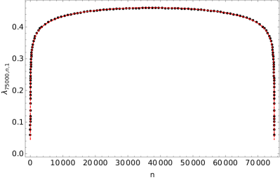
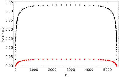
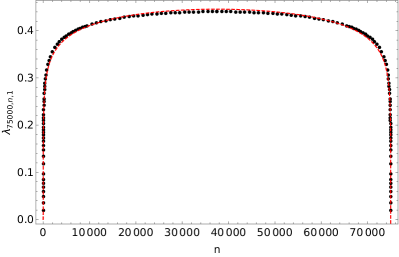
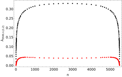
Figure 8: Lowest eigenvalue versus the blocked length $n$, for a massless open chain (top-left), a massive open chain (top-right), a massless closed chain (bottom left) and a massive closed chain (bottom right). See text.

C.3 Spectral flow of the largest eigenvalue

Most of the eigenvalues of the entangled density matrix except one $\lambda_{N,n,1}$, are exponentially small and randomly distributed following a Poisson distribution. This observation is consistent with the results in Liu and Zahed (2019) for the massless case. The exception is a large and collective eigenvalue,

$$\lambda_{N,n,1}\approx\bigg{(}1-e^{-S(am_{\theta}(T),n)}\bigg{)}$$ (59)

or equivalently

$$p_{l}[N,n,1]\approx e^{-S(am_{\theta}(T),n)}\bigg{(}1-e^{-S(am_{\theta}(T),n)}\bigg{)}^{l}$$

To derive (C.3), we retained the largest eigenvalue in (34) only, and assumed that $S_{E}$ is large, i.e.

$$\bigg{(}{\rm ln}(1-\lambda_{N,n,1})+\frac{\lambda_{N,n,1}}{1-\lambda_{N,n,1}}\,{\rm ln}\,\lambda_{N,n,1}\bigg{)}$$

$$=S_{E}+(e^{S_{E}}-1)\log(1-e^{-S_{E}})\approx S_{E}.$$

The largest eigenvalue (C.3) obeys the cascade equation

$$\frac{dp_{l}}{d{\rm ln}n}=\frac{1}{2}C(m_{\theta}(T)na)(-p_{l}+lp_{l-1})$$ (61)

with a rate fixed by the entropic function of $\frac{1}{2}$-Dirac massive fermion in (12).

The exact form of the bosonic entropy $S(am_{\theta}(T))$ in the continuum is not known analytically, although its entropic derivative (15) for large or small cuts is. It is also UV sensitive. As we suggested earlier, the central charge for free massive bosons, is to a good approximation analogous to the central charge of $\frac{1}{2}$-Dirac (Majorana) massive fermions as derived in Liu et al. (2023). Modulo a shift $\Lambda^{\prime}$, we have

$$S(am_{\theta}(T),n)\approx\frac{1}{6}\int_{0}^{1}dx\bigg{(}K_{0}\bigg{(}\frac{am_{\theta}(T)}{\sqrt{x(1-x)}}\bigg{)}-K_{0}\bigg{(}\frac{nam_{\theta}(T)}{\sqrt{x(1-x)}}\bigg{)}\bigg{)}\$$ (62)

In Fig. 8 top-left, we show the results for the lowest eigenvalue of the open and massless chain, with $N=75000$. The red dashed line is a fit to

$$\lambda_{N,n,1}=c_{1}\!\left(\!1-\exp\!\left(\!-c_{2}\log\!\left(\frac{N\sin\left(\frac{\pi n}{N}\right)}{\pi}\right)\!\right)\right.$$ (63)

with $c_{1}=0.829$ and $c_{2}=0.081$. Even though the result converges toward $c_{2}=1/6$, $N$ is still not large enough to be in the asymptotic regime, see Fig. 6. In Fig. 8 top-right, we show the results for the lowest two eigenvalues of an open and massive chain, with $N=5500$ and $m_{\theta}=0.001$.

In Fig. 8 bottom-left, we show the results for the massless and closed chain, with $N=75000$. The red dashed line is a fit to (63) with $N=50000$, $c_{1}=1.819$ and $c_{2}=0.02786$. In Fig. 8 bottom-right, we show the two lowest eigenvalues for a closed and massive chain with $N=5500$ and $m_{\theta}=0.001$. The spurious translational eigenvalue detailed in Appendix C, has been removed.

References

- Srednicki (1993) Mark Srednicki, “Entropy and area,” Phys. Rev. Lett. 71, 666–669 (1993), arXiv:hep-th/9303048 .
- Calabrese and Cardy (2004) Pasquale Calabrese and John L. Cardy, “Entanglement entropy and quantum field theory,” J. Stat. Mech. 0406, P06002 (2004), arXiv:hep-th/0405152 .
- Calabrese and Cardy (2009) Pasquale Calabrese and John Cardy, “Entanglement entropy and conformal field theory,” J. Phys. A 42, 504005 (2009), arXiv:0905.4013 [cond-mat.stat-mech] .
- Hastings (2007) M. B. Hastings, “An area law for one-dimensional quantum systems,” J. Stat. Mech. 0708, P08024 (2007), arXiv:0705.2024 [quant-ph] .
- Bauer et al. (2023) Christian W. Bauer et al., “Quantum Simulation for High-Energy Physics,” PRX Quantum 4, 027001 (2023), arXiv:2204.03381 [quant-ph] .
- Bekenstein (1981) Jacob D. Bekenstein, “Energy Cost of Information Transfer,” Phys. Rev. Lett. 46, 623–626 (1981).
- Stoffers and Zahed (2013) Alexander Stoffers and Ismail Zahed, “Holographic Pomeron and Entropy,” Phys. Rev. D 88, 025038 (2013), arXiv:1211.3077 [nucl-th] .
- Kharzeev and Levin (2017) Dmitri E. Kharzeev and Eugene M. Levin, “Deep inelastic scattering as a probe of entanglement,” Phys. Rev. D 95, 114008 (2017), arXiv:1702.03489 [hep-ph] .
- Ikeda et al. (2023a) Kazuki Ikeda, Dmitri E. Kharzeev, René Meyer, and Shuzhe Shi, “Detecting the critical point through entanglement in the schwinger model,” Phys. Rev. D 108, L091501 (2023a).
- ’t Hooft (1974) G. ’t Hooft, “A two-dimensional model for mesons,” Nuclear Physics B 75, 461–470 (1974).
- Schwinger (1962) Julian S. Schwinger, “Gauge Invariance and Mass. 2.” Phys. Rev. 128, 2425–2429 (1962).
- Ikeda et al. (2023b) Kazuki Ikeda, Dmitri E. Kharzeev, and Shuzhe Shi, “Non-linear chiral magnetic waves,” Phys. Rev. D 108, 074001 (2023b), arXiv:2305.05685 [hep-ph] .
- Florio et al. (2023) Adrien Florio, David Frenklakh, Kazuki Ikeda, Dmitri Kharzeev, Vladimir Korepin, Shuzhe Shi, and Kwangmin Yu, “Real-time nonperturbative dynamics of jet production in schwinger model: Quantum entanglement and vacuum modification,” Phys. Rev. Lett. 131, 021902 (2023).
- Ikeda et al. (2021) Kazuki Ikeda, Dmitri E. Kharzeev, and Yuta Kikuchi, “Real-time dynamics of Chern-Simons fluctuations near a critical point,” Phys. Rev. D 103, L071502 (2021), arXiv:2012.02926 [hep-ph] .
- Klco et al. (2018) N. Klco, E. F. Dumitrescu, A. J. McCaskey, T. D. Morris, R. C. Pooser, M. Sanz, E. Solano, P. Lougovski, and M. J. Savage, “Quantum-classical computation of schwinger model dynamics using quantum computers,” Phys. Rev. A 98, 032331 (2018).
- Sachs and Wipf (1992) Ivo Sachs and Andreas Wipf, “Finite temperature Schwinger model,” Helv. Phys. Acta 65, 652–678 (1992), arXiv:1005.1822 [hep-th] .
- Steele et al. (1995a) James V. Steele, J. J. M. Verbaarschot, and I. Zahed, “The Invariant fermion correlator in the Schwinger model on the torus,” Phys. Rev. D 51, 5915–5923 (1995a), arXiv:hep-th/9407125 .
- Byrnes et al. (2002) T. Byrnes, P. Sriganesh, R. J. Bursill, and C. J. Hamer, “Density matrix renormalization group approach to the massive Schwinger model,” Phys. Rev. D 66, 013002 (2002), arXiv:hep-lat/0202014 .
- Ohata (2023) Hiroki Ohata, “Phase diagram near the quantum critical point in Schwinger model at : analogy with quantum Ising chain,” (2023), arXiv:2311.04738 [hep-lat] .
- Hamer et al. (1982) C. J. Hamer, John B. Kogut, D. P. Crewther, and M. M. Mazzolini, “The Massive Schwinger Model on a Lattice: Background Field, Chiral Symmetry and the String Tension,” Nucl. Phys. B 208, 413–438 (1982).
- Schon and Thies (2000) Verena Schon and Michael Thies, “Emergence of Skyrme crystal in Gross-Neveu and ’t Hooft models at finite density,” Phys. Rev. D 62, 096002 (2000), arXiv:hep-th/0003195 .
- Park et al. (2000) Byung-Yoon Park, Mannque Rho, Andreas Wirzba, and Ismail Zahed, “Dense QCD: Overhauser or BCS pairing?” Phys. Rev. D 62, 034015 (2000), arXiv:hep-ph/9910347 .
- Rapp et al. (2001) Ralf Rapp, Edward V. Shuryak, and Ismail Zahed, “A Chiral crystal in cold QCD matter at intermediate densities?” Phys. Rev. D 63, 034008 (2001), arXiv:hep-ph/0008207 .
- Liu et al. (2023) Yizhuang Liu, Maciej A. Nowak, and Ismail Zahed, “Spatial entanglement in two-dimensional QCD: Renyi and Ryu-Takayanagi entropies,” Phys. Rev. D 107, 054010 (2023), arXiv:2205.06724 [hep-ph] .
- Casini and Huerta (2005) H. Casini and M. Huerta, “Entanglement and alpha entropies for a massive scalar field in two dimensions,” J. Stat. Mech. 0512, P12012 (2005), arXiv:cond-mat/0511014 .
- Goykhman (2015) Mikhail Goykhman, “Entanglement entropy in ’t Hooft model,” Phys. Rev. D 92, 025048 (2015), arXiv:1501.07590 [hep-th] .
- Casini et al. (2005) H. Casini, C. D. Fosco, and M. Huerta, “Entanglement and alpha entropies for a massive Dirac field in two dimensions,” J. Stat. Mech. 0507, P07007 (2005), arXiv:cond-mat/0505563 .
- Smilga (1992) Andrei V. Smilga, “On the fermion condensate in Schwinger model,” Phys. Lett. B 278, 371–376 (1992).
- Fayyazuddin et al. (1994) A. Fayyazuddin, T. H. Hansson, Maciej A. Nowak, J. J. M. Verbaarschot, and I. Zahed, “Finite temperature correlators in the Schwinger model,” Nucl. Phys. B 425, 553–578 (1994), arXiv:hep-ph/9312362 .
- Steele et al. (1995b) James V. Steele, Ajay Subramanian, and Ismail Zahed, “General correlation functions in the Schwinger model at zero and finite temperature,” Nucl. Phys. B 452, 545–562 (1995b), arXiv:hep-th/9503220 .
- Durr and Wipf (1997) S. Durr and A. Wipf, “Finite temperature Schwinger model with chirality breaking boundary conditions,” Annals Phys. 255, 333–361 (1997), arXiv:hep-th/9610241 .
- Bañuls et al. (2016) Mari Carmen Bañuls, Krzysztof Cichy, J. Ignacio Cirac, Karl Jansen, Stefan Kühn, and Hana Saito, “The multi-flavor Schwinger model with chemical potential - Overcoming the sign problem with Matrix Product States,” PoS LATTICE2016, 316 (2016), arXiv:1611.01458 [hep-lat] .
- Funcke et al. (2023) Lena Funcke, Tobias Hartung, Karl Jansen, Stefan Kühn, Marc-Oliver Pleinert, Stephan Schuster, and Joachim von Zanthier, “Exploring the phase structure of the multi-flavor Schwinger model with quantum computing,” PoS LATTICE2022, 020 (2023), arXiv:2211.13020 [quant-ph] .
- Dempsey et al. (2023a) Ross Dempsey, Igor R. Klebanov, Silviu S. Pufu, Benjamin T. Søgaard, and Bernardo Zan, “Phase Diagram of the Two-Flavor Schwinger Model at Zero Temperature,” (2023a), arXiv:2305.04437 [hep-th] .
- Dempsey et al. (2023b) Ross Dempsey, Igor R. Klebanov, Silviu S. Pufu, and Benjamin T. Søgaard, “Lattice Hamiltonian for Adjoint QCD2,” (2023b), arXiv:2311.09334 [hep-th] .
- Coleman (1975) Sidney R. Coleman, “The Quantum Sine-Gordon Equation as the Massive Thirring Model,” Phys. Rev. D 11, 2088 (1975).
- Liu and Zahed (2019) Yizhuang Liu and Ismail Zahed, “Entanglement in Regge scattering using the AdS/CFT correspondence,” Phys. Rev. D 100, 046005 (2019), arXiv:1803.09157 [hep-ph] .