Lattice aggregations of boxes and symmetric functions

Abstract.

We introduce two lattice growth models: aggregation of $l$-dimensional boxes and aggregation of partitions with $l$ parts. We describe properties of the models: the parameter set of aggregations, the moments of the random variable of the number of growth directions, asymptotical behavior of proportions of the most frequent transitions of two- and three-dimensional self-aggregations.

1. Introduction

Growth processes, and, in particular, aggregations of randomly moving particles and clusters are studied by a wide variety of theoretical models, experiments, and numerical simulations (see [5, 9, 10, 11, 16, 15] for examples related to the discussion here). Advances in computer technology and fractal geometry allowed researchers to describe many important growth parameters, such as fractal dimension, shapes, kinetics of formation. These studies show that with all the simplicity of the growth rules, the result is “a devilishly difficult model to solve, even approximately”, as it is emotionally expressed in [11].

For this reason, computational and experimental methods remain as the main investigation instruments of aggregation processes, while theoretical studies are restricted to significant simplifications and assumptions on the parameters. Yet, simplified analytical models give valuable insight into core characteristics of growth process.

In this note we introduce and study analytically a simplified growth model that is inspired by diffusion limited cluster aggregation (DLCA) models. In such models, once two randomly moving in a medium clusters attach to each other, they form a new cluster that continues to move and eventually finds other clusters to aggregate [11, 15].

In our simplified model the $n$-dimensional clusters are represented by $n$-dimensional rectangular boxes. Substitution of an object by an axis-aligned minimal bounding box is commonly used in approximation theory, since it leads to a less expensive, quick and sufficient evaluation of desired properties of the object. Two boxes produce on attachment a new bigger box by the procedure described in Section 3. The focus of this study is on the local statistical properties of the aggregates shapes, while the fractal nature of aggregates is “forgotten” in this model. This is not a conventional approach to the DLCA investigation, since, as it is pointed out in [11], the large-scale fractal structures of a cluster is dominated by non-local effects. Yet, we advocate here for the study of local growth properties, since, as we will see below, they provide interesting combinatorics.

The paper is organized as follows. A particular inspiration for our considerations comes from the observations in [7, 12], where DLCA numerical simulations describe the shapes of aggregates by inscribing them in the minimal bounding boxes and measuring the ratios of the side lengths of these boxes. In Section 2 we recall the interesting phenomena on the proportions of clusters that was observed in these papers.

In Section 3 from the definition of aggregation of boxes we deduce the basic properties of the process and describe the parameter set of possible attachments.

In Section 4 we describe the random variable of the number of directions in which an $n$-dimensional box grows under aggregation. We compute probabilities and the generating function of the moments in terms of elementary symmetric functions. In Section 5 we apply the results of the previous section to the aggregation of a box with a “particle” represented by a unit box.

In Section 6 we introduce the second model of aggregations of boxes up to equivalence of rotations, which defines families of transitional probabilities on the set of partitions of $l$ parts.

In Section 7 we come back to the observations outlined in Section 2 and describe the process of self-aggregation of partitions of the highest transitional probabilities. It turns out, that in two-dimensional case such transitions stabilize to a Fibonacci type sequence, which immediately implies the asymptotical limit on the ratios of side lengths of the boxes. In three-dimensional case a stabilizing sequence does not exist in general.

1.1. Acknowledgement

The author is very grateful to Prof. C. M. Sorensen for sharing valuable insights and providing detailed explanations on DLCA and RHA models. She would like to thank Prof. A. Chakrabarti for helpful discussions on the project. She also thanks Jasmine Hunt, for her undergraduate research project findings that made essential contribution to calculations of Table 3, and to Abhinav Chand and James Hyun, for writing a code that the author used to check her calculations in Table 10 and Figures 10-12. The research is supported by the the Simons Foundation Travel Support for Mathematicians grant MP-TSM-00002544.

2. Motivations: interpretations of peak values DLCA and RHM proportion distributions

From the vast variety of DLA and DLCA studies, we would like to recall the observations in [7, 12] that served as a special motivation for introduced here models, and, in particular, for the study of self-aggregations with the highest transitional probabilities in Section 7.

In [7] two computer simulation models are investigated: the diffusion limited cluster-cluster aggregation model (DLCA), and the restricted hierarchical model (RHM). The later one admits more theoretical analysis and is used to support an interesting interpretation of the maximal value point of certain probability distributions of the first model. Both models measure proportions of rectangular boxes circumscribed about aggregated clusters.

The DLCA simulation starts with $10^{6}$ monomers placed in a box. At each step, after the number of clusters is counted, a random cluster is chosen and moved in a random direction at a distance of one monomer diameter. Probability of this movement depends on the number of clusters and the size of the chosen cluster. On the collision, clusters irreversibly stick together, and the number of clusters goes down by one. In addition to calculation of fractal dimensions, the authors provide distributions of shapes of the $l$-dimensional aggregates ($l=2,3$) by comparing their “lengths” in $l$ perpendicular directions.

In two-dimensional case, let $L_{1}\geq L_{2}$ be the side lengths of a minimal bounding box of a cluster. In [7] the distribution of ratios $L_{1}/L_{2}$ for the set of the results of the DLCA simulation is computed. The computations show that the maximal value of this distribution is achieved at $L_{1}/L_{2}=1.63\pm 0.34$. Similarly, in three-dimensional case, let $L_{1}\geq L_{2}\geq L_{3}$ be the side lengths of the minimal bounding box of a cluster. According to [7], distributions of ratios $L_{i}/L_{j}$ ($i<j$) peaked at the values $L_{1}/L_{2}=1.46\pm 0.27$, $L_{2}/L_{3}=1.35\pm 0.24$ and $L_{1}/L_{3}=2.14\pm 0.27$.

The authors suggest a very interesting interpretation of these experimental values as approximations of irrational constants, $\varphi$, $\psi$ and $\psi^{2}$, where $\varphi\simeq 1.618$. is a root of $\varphi^{2}=\varphi+1$, and $\psi\simeq 1.465$ is a cubic root of $\psi^{3}=\psi^{2}+1$. This is a remarkable suggestion, since a natural presence of an irrational number would indicate that the peak value point of the distribution depends not so much on a physical input, but rather on mathematical properties of the model. In the support of this conjecture, a restricted hierarchical model (RHM) was studied in [12]. This model is more analytical and has a significantly smaller number of possible aggregation results. It is based on the aggregation of cloned clusters under the “side-to-end’ condition: the longest side of the original cluster should be necessarily linked with the shortest side of its clone. The side-to-end aggregations similarly appear as T-model in [14], where aggregating clusters are modeled by ellipses always sticking together to create a T-shape, along with the averaged model, where non-zero probabilities are limited only to three types of attachments. In Section 7 we relate interpretations of the peak value points of distributions of proportions of clusters [7, 12] to the most frequent transitions of self-aggregations of partitions.

3. Aggregations of boxes: definitions and properties

3.1. Two growth models

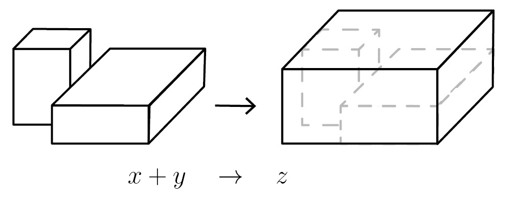
Figure 1. Aggregation of three-dimensional boxes.

In the growth models of this note an $l$-dimensional cluster is represented by an $l$-dimensional rectangular box those movements are aligned with an integer lattice ${\mathbb{Z}}^{l}$. Two boxes attach to each other along the lattice to produce a new box (Figure 1). For the purpose of counting, there are two possible variations (Figure 2):

1. Different orientations of a box are declared to represent different clusters. In this case each cluster is identified with an array of the side lengths of the box $x=(x_{1},\dots,x_{l})\in{\mathbb{Z}}^{l}_{>0}$ written in a particular order. We refer to this growth model as aggregation of boxes.

2. Alternatively, one can identify all rotations of a box to be the same cluster. As it is explained in Section 6, in this case each cluster is identified with a partition $\lambda=(\lambda_{1}\geq\dots\geq\lambda_{l}>0)$, $\lambda_{i}\in{\mathbb{Z}}_{>0}$. This model is called aggregation of partitions.

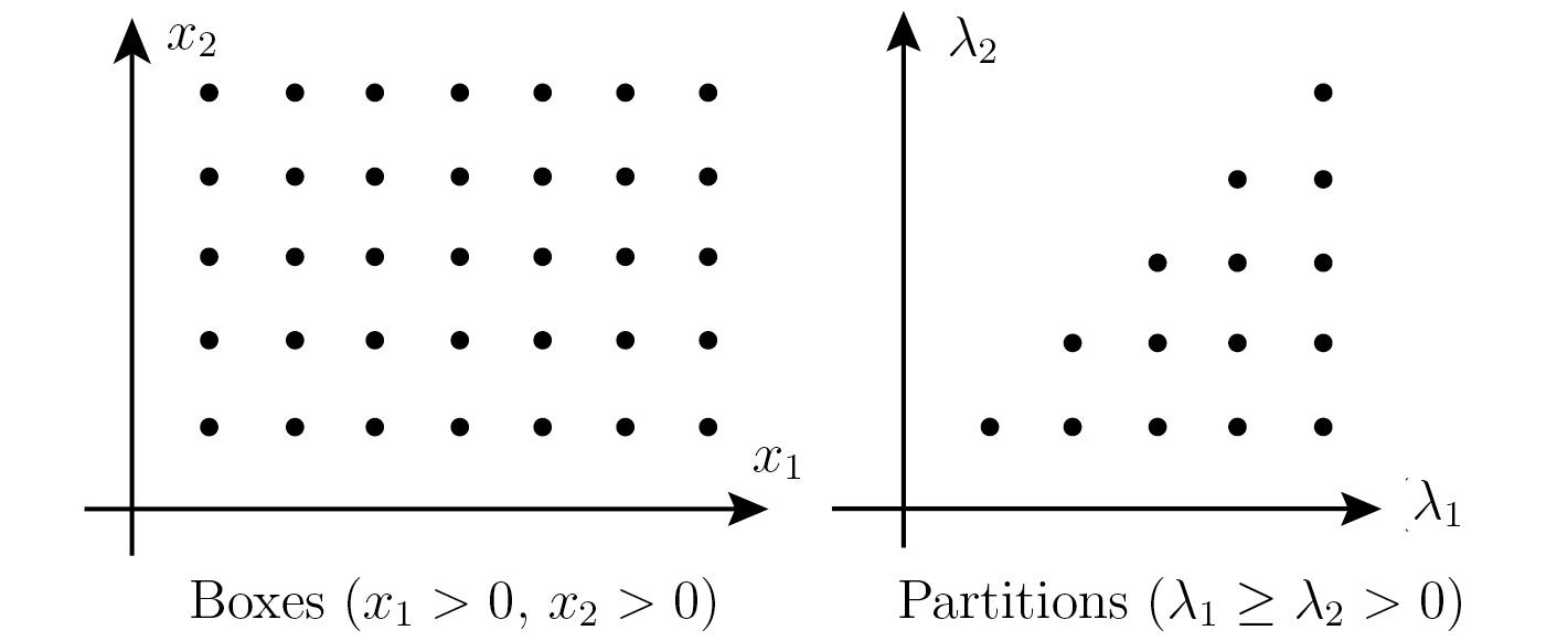
Figure 2. Enumeration of boxes and partitions in two-dimensional models.

In many applications the assumption that all rotations represent the same shape seem to be natural. Combinatorics of aggregations of partitions is more involved than combinatorics of aggregation of boxes, but still it is based on counting of contributing aggregations of rotated boxes. Hence, we aim to study both aggregation models. Our goal is to describe properties of these two models and to compare with studies of DLA models in [7], [12].

3.2. Aggregation of boxes

We fix an integer lattice ${\mathbb{Z}}^{l}\subset{\mathbb{R}}^{l}$ aligned with a Cartesian coordinate system. Let the origin of the coordinate system coincide with one of the vertices of the lattice.

Definition 3.1.

An $l$-dimensional box $x$ is a Cartesian product of $l$ parallel to the coordinate axes intervals with the integer lengths represented by the array $x=(x_{1},\dots,x_{l})\in{\mathbb{Z}}_{>0}^{l}$. Below we always assume that the endpoints of these intervals are placed at the vertices of the lattice.

Thus, we identify an $l$-dimensional box with a point of ${\mathbb{Z}}_{>0}^{l}$. For example, a rectangle of size $3$ by $5$ corresponds to a point $(3,5)$, and a rectangle of size $5$ by $3$ is a different point with coordinates $(5,3)$.

Let $x$ and $y$ be two $l$-dimensional boxes. The box $y$ is translated without rotations, moving around $x$, and producing a collection of new boxes by the following attachment procedure (Figure 1).

• Boxes $x$ and $y$ are placed next to each other, so that all their sides are aligned with the coordinate axes of the $l$-dimensional space, and vertices of both boxes are situated on the lattice ${\mathbb{Z}}^{l}$.

• The boxes must be in the attachment: their boundaries must contain at least one common lattice point.

• The union of the two attached boxes $x$ and $y$ is inscribed in a minimal bounding box $z$ aligned with the coordinate axes, as in Figure 1.

Definition 3.2.

We say that the box $z$ is a result of aggregation of two boxes $x$ and $y$, and write ‘$x+y\to z$’.

Various attachments of two boxes produce a number of possible results, and the sizes of resulting boxes may repeat for different attachments. Assuming that all attachments are equally likely, we introduce the probability distribution on all possible results $P^{z}_{xy}=P(x+y\to z)$ as the number of occurrences of a box $z$, divided by the total number of ways for $x$ and $y$ to aggregate.

Example 3.1.

There are 14 possible attachments of $x=(1,3)$ and $y=(1,2)$, and there are 14 possible attachments of $x=(1,3)$ and $y=(2,1)$. The probability distributions of aggregation results are given in Tables 1, 2.

$z$	$(2,5)$	$(2,4)$	$(2,3)$	$(1,5)$	otherwise
$P^{z}_{(1,3),(1,2)}$	$\frac{2}{7}$	$\frac{2}{7}$	$\frac{2}{7}$	$\frac{1}{7}$	$0$

Table 1. Results of aggregation $(1,3)+(1,2)$

$z$	$(3,4)$	$(3,3)$	$(2,4)$	otherwise
$P^{z}_{(1,3),(2,1)}$	$\frac{2}{7}$	$\frac{3}{7}$	$\frac{2}{7}$	0

Table 2. Results of aggregation $(1,3)+(2,1)$

3.3. Two-dimensional case: aggregation of rectangles

It is not difficult to compute frequencies of results of aggregation of any $2$-dimensional boxes $x=(x_{1},x_{2})$ and $y=(y_{1},y_{2})$. The total number of possible attachments of these rectangles is $|T|=2(x_{1}+x_{2}+y_{1}+y_{2})$ (see Proposition 3.2 for general formula). Probability distribution $P^{z}_{x,y}$ is provided in Table 3.

Result of aggregation $z=(z_{1},z_{2})$	Probability $P^{z}_{x,y}$
$(x_{1}+y_{1},x_{2}+y_{2}),$	$\frac{4}{|T|}$
$(x_{1}+y_{1}-s,y_{2}+x_{2}),\quad s=1,\dots,\min(x_{1},y_{1})-1$,	$\frac{4}{|T|}$
$(x_{1}+y_{1},x_{2}+y_{2}-s),\quad s=1,\dots,\min(x_{2},y_{2})-1$,	$\frac{4}{|T|}$
$(x_{1}+y_{1},\max(x_{2},y_{2}))$	$\frac{2|y_{2}-x_{2}|+2}{|T|}$
$(\max(x_{1},y_{1})\,,x_{2}+y_{2})$	$\frac{2|y_{1}-x_{1}|+2}{|T|}$
otherwise	0

Table 3. Probability distribution of aggregation of rectangles.

3.4. Basic properties of aggregation of boxes

The following properties of probability distributions immediately follow from the definition.

Proposition 3.1.

Let $x=(x_{1},\dots,x_{i},\dots,x_{l})$ and $y=(y_{1},\dots,y_{i},\dots y_{l})$ be two $l$-dimensional boxes.

1. $\sum_{z\in{\mathbb{Z}}^{l}_{>0}}P^{z}_{x,y}=1$.

2. $P^{z}_{x,y}=P^{z}_{y,x}$ for any $z\in{\mathbb{Z}}^{l}_{>0}$.

3. Let $x^{\prime}=(x_{1},\dots,y_{i},\dots,x_{l})$ and $y^{\prime}=(y_{1},\dots,x_{i},\dots y_{l})$ be a pair of boxes obtained from the original pair $x$ and $y$ by the swap of sides $x_{i}\leftrightarrow y_{i}$. Then both pairs of aggregating boxes have the same sets of results with the same probabilities:

   $$P^{z}_{x,y}=P^{z}_{x^{\prime},y^{\prime}}\quad\text{for any $z\in{\mathbb{Z}}^{l}_{>0}$.}$$

4. $P^{z}_{xy}\neq 0$ if and only if $z=(z_{1},\dots,z_{l})$ is within the range $max(x_{i},y_{i})\leq z_{i}\leq x_{i}+y_{i}$ for all $i\in\{1,\dots,l\}$.

3.5. Parameter set of aggregations

In this section we describe the parameter set of possible attachments of two $l$-dimensional boxes. This allows us to to compute the total number of aggregations for two boxes and compute some interesting probabilities.

Proposition 3.2.

1. Let $x=(x_{1},\dots,x_{l})$ and $y=(y_{1},\dots,y_{l})$ be two $l$-dimensional boxes.

2. Let $R_{x+y}$ be an $l$-dimensional box of size $(x_{1}+y_{1})\times\dots\times(x_{l}+y_{l})$ fixed in the position with one vertex in the origin:

   $$R_{x+y}=\{(s_{1},\dots s_{l})|0\leq s_{i}\leq x_{i}+y_{i}\}.$$

   The set of possible attachments of boxes $x$ and $y$ in the process of their aggregation is in one-to-one correspondence with the set $T$ of all integer points of the boundary of $R_{x+y}$:

   $$T={\mathbb{Z}}^{l}\cap\partial R_{x+y}$$

3. Thus, number $|T|=|\{z|x+y\to z\}|$ of all possible results of aggregations $x+y\to z$ counted with multiplicities is given by

   $$|T|=\prod_{i=1}^{l}(x_{i}+y_{i}+1)-\prod_{i=1}^{l}(x_{i}+y_{i}-1).$$

4. Let $s=(s_{1},s_{2},\dots,s_{l})\in T$ be one of the points of the parameter set producing the result of aggregation $z(s)$. Then $z(s)=(z_{x_{1},y_{1}}(s_{1}),\dots z_{x_{l},y_{l}}(s_{l}))$, where

   (3.1) $$z_{x_{i},y_{i}}(s_{i})=\max(x_{i},y_{i},x_{i}+y_{i}-s_{i},s_{i}),$$

   illustrated in Figure 3.

   

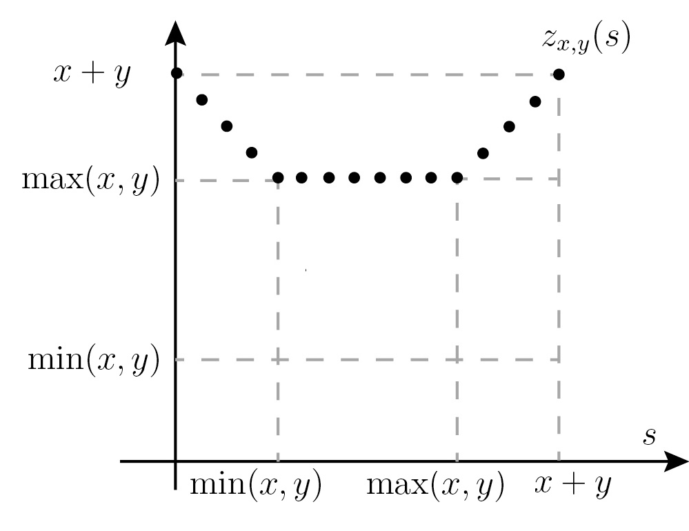
   Figure 3. Graph of $z_{xy}(s)$ of side lengths of results of aggregations.

Proof.

1. Recall that aggregations $x+y\to z$ are produced by moving $y$ around $x$ in an attachment. Each position of $y$ defines an aggregation result $z$, and at the same time, each position of $y$ is completely defined by a position of any vertex of $y$. Mark a vertex of $y$ and follow its movement during the aggregation procedure. It is clear that the position of this vertex runs through all integer boundary points of an $(x_{1}+y_{1})\times\dots\times(x_{l}+y_{l})$ box. Thus the set of attachments of $x$ and $y$ is parametrized by integer boundary points of such box. We denote this parameter box as $R_{x+y}$ and place it in the origin for the convenience of formulas and proofs below.

2. The number $|T|$ of the integer boundary points equals the difference between the number of all integer points of this box $\prod_{i=1}^{l}(x_{i}+y_{i}+1)$ and the number of interior integer points of this box $\prod_{i=1}^{l}(x_{i}+y_{i}-1)$.

3. Let $x_{i}$ and $y_{i}$ be the $i$-th sizes of aggregating boxes. From Proposition 3.1 we can assume that $y_{i}\geq x_{i}$. Let $A$ be a marked vertex of the box as in the proof of (1). Possible values of coordinates $(s_{1},\dots,s_{l})$ of $A$ parametrize all possible attachments of $x$ and $y$. Since $y$ moves along each non-attaching coordinate independently, it is sufficient to prove (3) just for the projection on one coordinate, see Figure 4. As the box $y$ moves, the coordinate $s_{i}$ runs through the values between $0$ and $x_{i}+y_{i}$. The corresponding size $z_{i}(s_{i})$ of the aggregation result starts with the maximal possible value $x_{i}+y_{i}$ then linearly drops down to the value of $y_{i}$, remains on the same level until $s_{i}=y_{i}$, after that it again grows linearly until reaches the value $z_{i}(x_{i}+y_{i})=x_{i}+y_{i}$. The resulting function for $z_{i}(s_{i})$ is exactly of the form (3.1).

   

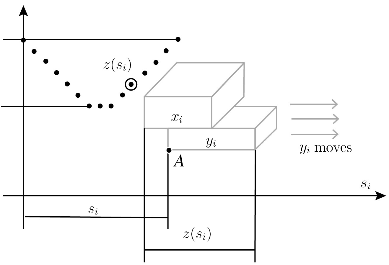
   Figure 4. Varying $s_{i}$ by moving edge $y_{i}$ along the edge $x_{i}$ and measuring the combined size $z(s_{i})$.

∎

Example 3.2.

Figure 5 gives an example of the parameter set for the aggregations $(1,1,4)+(5,2,3)$.

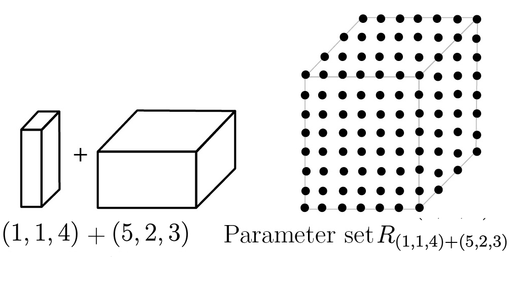
Figure 5. Possible attachments of $(1,1,4)$ and $(5,2,3)$ is parametrized by integer points on the boundary of a box $R_{(1,1,4)+(5,2,3)}=(6,3,7)$.

Example 3.3.

If $l=2$, then the total number of aggregations with multiplicities is

$$|T|=2(x_{1}+x_{2}+y_{1}+y_{2})$$

If $l=3$, then

$$|T|=2+2(x_{1}+y_{1})(x_{2}+y_{2})+2(x_{1}+y_{1})(x_{3}+y_{3})+2(x_{2}+y_{2})(x_{3}+y_{3}).$$

4. The number of growth directions

4.1. Growth of a box in $k$ particular directions

For the simplicity of notations, by Proposition 3.1, we assume in this section that all $x_{i}\geq y_{i}$, $(i=1,\dots,l)$. Then a side length $z_{i}$ of a result of aggregation $x+y\to z$ either stays the same $z_{i}=x_{i}$ or grows $z_{i}=x_{i}+t_{i}$,  $0<t_{i}\leq y_{i}$. Our goal is to describe the random variable that assigns to each result of aggregation $z$ the number of sides that have changed their lengths from the side lengths of $x$.

Proposition 4.1.

Let $z$ be a result of aggregation of $x+y\to z$, where $x_{i}\geq y_{i}$ for all $i=1,\dots,l$. Let $1\leq i_{1}<\dots<i_{k}\leq l$, $1\leq k\leq l$. Denote as $P(i_{1},\dots i_{k})$ the probability that $z$ grows from $x$ in the directions $\{i_{1},\dots,i_{k}\}$:

$$P(i_{1},\dots,i_{k})=P(z_{j}>x_{j}\,\text{if and only if }\,j\in\{i_{1},\dots,i_{k}\}).$$

Then

(4.1) $$P(i_{1},\dots,i_{k})=\frac{2^{k}}{|T|}\left(\prod_{j\in\{i_{1},\dots,i_{k}\}}y_{j}-\prod_{j\in\{i_{1},\dots,i_{k}\}}(y_{j}-1)\right)\prod_{j\notin\{i_{1},\dots,i_{k}\}}(x_{j}-y_{j}+1).$$

Proof.

Without loss of generality we can assume that $\{i_{1},\dots,i_{k}\}=\{1,\dots,k\}$. Each result $z(s)$ that is different from $x$ in the first $k$ places is generated by attachments that correspond to parameters $s_{j}\in[0,y_{j}-1]\cup[x_{j}+1,x_{j}+y_{j}]$ for $j=1,\dots,k$ and $s_{j}\in[y_{j},x_{j}]$ for $j=k+1,\dots,l$, under the condition that there is an attachment in at least one coordinate: for at least one $j\in\{1,\dots k\}$, $s_{j}=0$ or $s_{j}=x_{j}+y_{j}$.

Assume for a moment that for all $j\in\{1,\dots,k\}$, $s_{j}\in[0,y_{j}-1]$. Using the condition that at least one of $s_{j}=0$ among these $j\in\{1,\dots k\}$, and that $s_{j}\in[y_{j},x_{j}]$ for $j=k+1,\dots,l$, we conclude that this set of parameters is identified with a set of integer points of “the exterior” part of the boundary the $l$-dimensional box $[0,y_{1}-1]\times\dots\times[0,y_{k}-1]\times[y_{k+1},x_{k+1}]\dots\times[y_{l},x_{l}]$. Figure 6 illustrates this statement in three-dimensional case. The integer points of the boundary of the box $[0,x_{1}+y_{1}]\times[0,x_{2}+y_{2}]\times[0,x_{3}+y_{3}]$ represent the set $T$ of all parameters of attachments. The shaded parts of the boundary represent parameters $s$ that correspond to:

• $k=3$, $0\leq s_{j}<y_{j}$ for $j\in\{1,2,3\}$, and either $s_{1}=0$, or $s_{2}=0$, or $s_{3}=0$.

• $k=2$, $0\leq s_{j}<y_{j}$ for $j\in\{1,2\}$, and either $s_{1}=0$, or $s_{2}=0$, and $y_{3}\leq s_{3}\leq x_{3}$.

• $k=1$, $s_{1}=0$, and for $j\in\{2,3\}$ $y_{j}\leq s_{j}\leq x_{j}$.

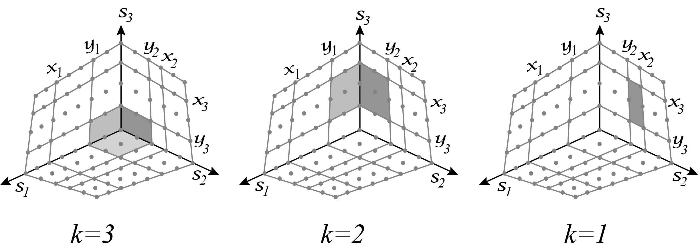
Figure 6. Parameters for changes in $k=3,2,1$ directions.

The cardinality of the described subset of parameters is given by the difference of the number of integer points in the box $[0,y_{1}-1]\times\dots\times[0,y_{k}-1]\times[y_{k+1},x_{k+1}]\dots\times[y_{l},x_{l}]$ and the box $[1,y_{1}-1]\times\dots\times[1,y_{k}-1]\times[y_{k+1},x_{k+1}]\dots\times[y_{l},x_{l}]$, which is

$$\prod_{j=k+1}^{l}(x_{j}-y_{j}+1)\left(\prod_{j=1}^{k}y_{j}-\prod_{j=1}^{k}(y_{j}-1)\right).$$

Allowing each $s_{j}$, $j=1,\dots,k$ to vary through two options of intervals, $[0,y_{j}-1]$, or $[x_{j}+1,x_{j}+y_{j}]$, we get $2^{k}$ copies of the same subset to conclude that

$$P(1,\dots,k)=\frac{2^{k}}{|T|}\prod_{j=k+1}^{l}(x_{j}-y_{j}+1)\left(\prod_{j=1}^{k}y_{j}-\prod_{j=1}^{k}(y_{j}-1)\right).$$

Statement (4.1) follows by permuting the indices $\{1,\dots,k\}$ to get $\{i_{1},\dots,i_{k}\}$.

∎

4.2. Elementary symmetric functions

Further combinatorics of this random variable is effectively described in the language of symmetric polynomials [8].

Definition 4.1.

For $k=1,2,\dots$ the elementary symmetric polynomial $E_{k}(a_{1},\dots,a_{n})$ in $n$ variables $(a_{1},\dots,a_{n})$, $n\geq k$, is defined by

$$E_{k}(a_{1},\dots,a_{n})=\sum_{1\leq i_{1}<\dots<i_{k}\leq n}a_{i_{1}}\dots a_{i_{k}},$$

and $E_{0}=1$.

A well-known identity relates elementary symmetric functions and expansion of a polynomial with roots $a_{1},\dots,a_{n}$:

$$\prod_{{j=1}}^{n}(u-a_{j})=\sum_{k=0}^{n}(-1)^{n-k}E_{n-k}(a_{1},\dots,a_{n})u^{k}.$$

For $1\leq i_{1}<\dots<i_{k}\leq l$, $1\leq k\leq l$, $a,b\in{\mathbb{R}}^{l}$, let

$$r_{i_{1},\dots,i_{k}}(a,b)=\prod_{j\notin\{i_{1},\dots,i_{k}\}}a_{j}\prod_{j\in\{i_{1},\dots,i_{k}\}}b_{j},$$

$$R_{k}(a,b)=\sum_{1\leq i_{1}<\dots<i_{k}\leq l}r_{i_{1},\dots,i_{k}}(a,b),\quad\mathcal{R}(a,b)[u]=\sum_{k=1}^{l}u^{k}R_{k}(a,b).$$

Lemma 4.1.

1. $$\mathcal{R}(a,b)[u]=\prod_{i=1}^{l}(a_{i}+ub_{i})$$

2. $R_{k}(a,b)$ can be expressed through elementary symmetric functions:

   $$R_{k}(a,b)=b_{1}\dots b_{l}E_{l-k}\left(\frac{a_{1}}{b_{1}},\dots,\frac{a_{l}}{b_{l}}\right)=a_{1}\dots a_{l}E_{k}\left(\frac{b_{1}}{a_{1}},\dots,\frac{b_{l}}{a_{l}}\right).$$

Proof.

1. Observe that $u^{k}r_{i_{1},\dots,i_{k}}(a,b)=r_{i_{1},\dots,i_{k}}(a,ub)$, hence $u^{k}R_{k}(a,b)=R_{k}(a,ub)$, and it is enough to show that

   $$\mathcal{R}(a,b)[1]=\sum_{k=0}^{l}\sum_{1\leq i_{1}<\dots<i_{k}\leq l}r_{i_{1},\dots,i_{k}}(a,b)=\prod_{i=1}^{l}(a_{i}+b_{i}).$$

   Consider an $l$-dimensional box of sizes $(a_{1}+b_{1},\dots,a_{l}+b_{l})$. Clearly, its volume is $\prod_{i=1}^{l}(a_{i}+b_{i})$. Divide each edge of this box into two parts, of lengths $a_{i}$ and $b_{i}$, and cut the box into smaller boxes, as illustrated in the Figure 7 for $l=3$. Then the total volume is the sum of volumes of smaller boxes, which are exactly of the form $r_{i_{1},\dots,i_{k}}(a,b)$.

   

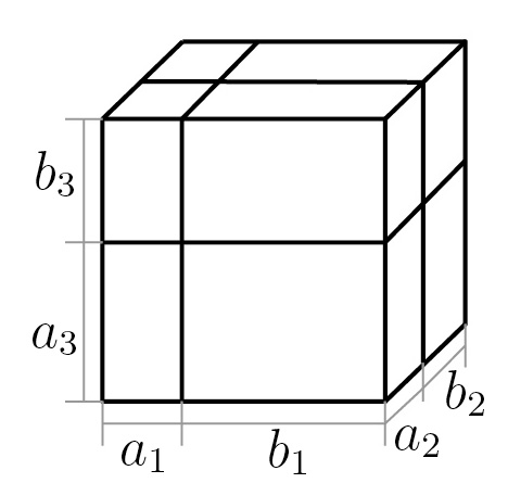
   Figure 7. Cutting the box by division of edges into sum of lengths $a_{i}$ and $b_{i}$,

∎

4.3. Random variable of the number of directions growth

Through this section we again assume that $x_{i}\geq y_{i}$ for all $i=1,\dots,l$. Let $X$ be the random variable that assigns to a result of aggregation $x+y\to z$, the number of side lengths of $z$ that are different from $x$. Then

$$P(X=k)=\sum_{1\leq i_{1}<\dots<i_{k}\leq l}P(i_{1},\dots,i_{k}),$$

where in the introduced above notations

$$P(i_{1},\dots,i_{k})=\frac{2^{k}}{|T|}\left(r_{i_{1},\dots,i_{k}}(x-y+1^{l},y)-r_{i_{1},\dots,i_{k}}(x-y+1^{l},y-1^{l})\right)$$

with $1^{l}=(1,\dots,1)\in{\mathbb{Z}}^{l}$. Then we get

Proposition 4.2.

Let $x_{i}\geq y_{i}$ for all $i=1,\dots,l$. Then the probability that a result of aggregation of $x$ and $y$ is longer than original box $x$ in $k$ directions is given by

$$P(X=k) =\frac{2^{k}}{|T|}\left(R_{k}(x-y+1^{l},y)-R_{k}(x-y+1^{l},y-1^{l})\right)$$

$$=\frac{2^{k}\prod_{i=1}^{l}(x_{i}-y_{i}+1)}{|T|}\left(E_{k}\left(\frac{y}{x-y+1^{l}}\right)-E_{k}\left(\frac{y-1^{l}}{x-y+1^{l}}\right)\right),$$

where we used short notations

$$E_{k}\left(\frac{y}{x-y+1^{l}}\right)=E_{k}\left(\frac{y_{1}}{x_{1}-y_{1}+1},\dots,\frac{y_{l}}{x_{l}-y_{l}+1}\right)$$

and

$$E_{k}\left(\frac{y-1^{l}}{x-y+1^{l}}\right)=E_{k}\left(\frac{y_{1}-1}{x_{1}-y_{1}+1},\dots,\frac{y_{l}-1}{x_{l}-y_{l}+1}\right).$$

The moments of the random variable $X$ are defined in a standard way:

$$M^{p}=\sum_{k=1}^{l}k^{p}\,P(X=k).$$

Proposition 4.3.

The moments $M^{p}$ of $X$ can be computed by the formula

$$M^{p} =\frac{(u\,\partial_{u})^{p}\mathcal{M}(u))}{\mathcal{M}(u)}|_{u=2},$$

where

(4.2) $$\mathcal{M}(u) =\prod_{i=1}^{l}\left(1+\frac{y_{i}u}{x_{i}-y_{i}+1}\right)-\prod_{i=1}^{l}\left(1+\frac{(y_{i}-1)u}{x_{i}-y_{i}+1}\right).$$

Proof.

From the definition of moments we deduce:

$$M^{p} =\frac{1}{|T|}\sum_{k=1}^{l}k^{p}\,{2^{k}}R_{k}(x-y+1^{l},y)-\frac{1}{|T|}\sum_{k=1}^{l}k^{p}\,{2^{k}}R_{k}(x-y+1^{l},y-1^{l})$$

$$=\frac{1}{|T|}\left(\sum_{k=1}^{l}k^{p}\,{u^{k}}R_{k}(a,b)|_{a=x-y+1^{l},b=y,u=2}-\sum_{k=1}^{l}k^{p}\,{u^{k}}R_{k}(a,b)|_{a=x-y+1^{l},b=y-1^{l},u=2}\right).$$

Let $(k)_{r}=k(k-1)\dots(k-r+1)$. Recall that $\partial_{u}^{r}(u^{k})=(k)_{r}u^{k-r}$, $u^{r}\partial_{u}^{r}=(u\partial_{u})_{r}$, and that $\quad k^{p}=\sum_{r=0}^{p}S(p,r)(k)_{r}$, where $S(p,r)$ are Stirling numbers of the second kind. We get

$$\sum_{k=1}^{l}{k^{p}\,u^{k}R_{k}(a,b)} =\sum_{k=1}^{l}\sum_{r=0}^{p}S(p,r)(k)_{r}\,u^{k}R_{k}(a,b)$$

$$=\sum_{r=0}^{p}S(p,r)u^{r}\sum_{k=1}^{l}(k)_{r}\,u^{k-r}R_{k}(a,b)$$

$$=\sum_{r=0}^{p}S(p,r)u^{r}\partial_{u}^{r}\left(\sum_{k=1}^{l}u^{k}R_{k}(a,b)\right)$$

$$=(u\,\partial_{u})^{p}\left(\sum_{k=1}^{l}u^{k}R_{k}(a,b))\right)=(u\,\partial_{u})^{p}\mathcal{R}(a,b)[u].$$

Then

(4.3) $$M^{p} =\frac{1}{|T|}(u\,\partial_{u})^{p}\left(\mathcal{R}(x-y+1^{l},y)[u]-\mathcal{R}(x-y+1^{l},y-1^{l})[u]\right)|_{u=2}.$$

Note that

$$|T|={\prod_{i}(x_{i}+y_{i}+1)-\prod_{i}(x_{i}+y_{i}-1)}=\left(\mathcal{R}(x-y+1^{l},y)[u]-\mathcal{R}(x-y+1^{l},y-1^{l})[u]\right)|_{u=2}.$$

To compete the proof express everything in (4.3) through

$$\mathcal{M}(u) =\frac{1}{\prod(x_{i}-y_{i}+1)}\left(\mathcal{R}(x-y+1^{l},y)[u]-\mathcal{R}(x-y+1^{l},y-1^{l})[u]\right)$$

$$=\prod_{i=1}^{l}\left(1+\frac{uy_{i}}{x_{i}-y_{i}+1}\right)-\prod_{i=1}^{l}\left(1+\frac{u(y_{i}-1)}{x_{i}-y_{i}+1}\right).$$

∎

Corollary 4.1.

Let $x_{i}\geq y_{i}$ for all $i=1,\dots,l$. On average a result of aggregation of $x$ and $y$ is longer than $x$ in $M$ directions, where

$$M=2\ln(\mathcal{M}(u))^{\prime}|_{u=2}$$

and $\mathcal{M}(u)$ is given by (4.2).

5. Aggregation with a unit box

5.1. Properties of aggregation with a unit box.

In case of aggregation with a “particle”, that is with a unit box $y=(1^{l})=(1,\dots,1)$, formulas of Section 4 simplify to nice expressions. We summarize them in Proposition 5.1. Clearly, each result $z$ of aggregation $x+(1^{l})\to z$ is an $l$-dimensional box $z=(z_{1},\dots,z_{l})$ those side lengths either remain the same $z_{i}=x_{i}$, or grow by one, $z_{i}=x_{i}+1$.

Proposition 5.1.

In the $l$-dimensional space consider the process of the aggregation of boxes $x+1^{l}\to z$. Then

1. The total number of ways for a particle $1^{l}$ to attach to the box $x$ is

   $$|T|=\prod_{i=1}^{l}(x_{i}+2)-\prod_{i=1}^{l}x_{i}$$

2. Each result of aggregation $x+1^{l}\to z$ is of the form $z=x+e_{i_{1}}+\dots+e_{i_{k}}$, where $e_{i}=(0,\dots,\underset{i}{1}\dots,0)$, $1\leq i_{1}<\dots<i_{k}\leq l$, and $1\leq k\leq l$. Transitional probabilities are given by

   (5.1) $$P_{x,1^{l}}^{x+e_{i_{1}}+\dots+e_{i_{k}}}=P(i_{1},\dots,i_{k})=\frac{2^{k}\,x_{1}\dots x_{l}}{x_{i_{1}}\dots x_{i_{k}}|T|}.$$

3. Probability that the resulting box will grow in size by $1$ in $k$ directions ($k=1,2,\dots,l$) is given by the formula

   (5.2) $$P(X=k)=\frac{2^{k}E_{l-k}(x_{1},\dots,x_{l})}{|T|},$$

   where $E_{s}(x_{1},\dots,x_{l})=\sum_{1\leq i_{1}<\dots<\i_{s}\leq l}x_{i_{1}}\dots x_{i_{s}}$ is the $s$-th elementary symmetric polynomial.

4. On average through the aggregation with a particle a box $x$ grows in size in $M$ directions, where

   $$M=\frac{\sum_{i=1}^{l}\frac{2}{2+x_{i}}}{1-\prod_{i=1}^{l}\frac{x_{i}}{x_{i}+2}},$$

Proof.

The statements follow by substitution $y=(1^{l})$ in Propositions 3.2 nd 4.1. For the last statement, we compute the average number of directions as the first moment of variable $X$ using Corollary 4.1:

$$M =\frac{u\partial_{u}\left(\prod_{i=1}^{l}(1+\frac{u}{x_{i}})-1\right)}{\prod_{i=1}^{l}(1+\frac{u}{x_{i}})-1}|_{u=2}=\frac{\sum_{i=1}^{l}\frac{u}{u+x_{i}}\prod_{i=1}^{l}\left(1+\frac{u}{x_{i}}\right)}{\prod_{i=1}^{l}(1+\frac{u}{x_{i}})-1}|_{u=2}$$

$$=\frac{\sum_{i=1}^{l}\frac{u}{u+x_{i}}}{1-\prod_{i=1}^{l}\frac{x_{i}}{x_{i}+u}}|_{u=2}=\frac{\sum_{i=1}^{l}\frac{2}{2+x_{i}}}{1-\prod_{i=1}^{l}\frac{x_{i}}{x_{i}+2}},$$

where we used ([8] I, (2.10^′)):

$$u\partial_{u}\prod_{i=1}^{l}\left(1+\frac{u}{a_{i}}\right)=\sum_{i=1}^{l}\frac{u}{u+a_{i}}\prod_{i=1}^{l}\left(1+\frac{u}{a_{i}}\right).$$

∎

Example 5.1.

$l=2$

$$M=\frac{x_{1}+x_{2}+4}{x_{1}+x_{2}+2}=1+\frac{2}{x_{1}+x_{2}+2}.$$

Note that in this case the average number of directions depends on the perimeter of $x$, but does not depend on individual lengths. As the perimeter grows to infinity, on average the rectangle will will grow in one direction at each transition. Note also that $M<2$ for any rectangle $x$.

Example 5.2.

$l=3$

$$M =\frac{x_{1}x_{2}+x_{1}x_{3}+x_{2}x_{3}+4(x_{1}+x_{2}+x_{3})+12}{x_{1}x_{2}+x_{1}x_{3}+x_{2}x_{3}+2(x_{1}+x_{2}+x_{3})+4}$$

$$=1+\frac{2(x_{1}+x_{2}+x_{3})+8}{x_{1}x_{2}+x_{1}x_{3}+x_{2}x_{3}+2(x_{1}+x_{2}+x_{3})+4}.$$

If $x$ is not a unit cube$(1,1,1)$, then $x_{1}x_{2}+x_{1}x_{3}+x_{2}x_{3}>4$, and again we get $M<2$.

Corollary 5.1.

Assume that $x_{i}=O(N)$ as $N\to\infty$ for all $i=1,\dots,l$.Then asymptotically on average the size of the box $x$ grows in just in 1 direction by the aggregation with a unit box.

Proof.

With $x_{i}=O(N)$ as $N\to\infty$ for all $i=1,\dots,l$ we can write that

$$M=\frac{2\sum_{i=1}^{l}\prod_{j\neq i}{(x_{j}+2)}}{\prod_{i=1}^{l}{(x_{i}+2)}-\prod_{i=1}^{l}{x_{i}}}\to 1\quad\text{ when $N\to\infty$.}$$

∎

5.2. Markov chain

Repeating aggregation with a unit box $y=(1^{l})$ one defines a Markov chain on the space of $l$-dimensional boxes with transition probabilities $\{p_{xz}=P_{x,(1^{l})}^{z}\}$, given by (5.1). Within standard definitions [4], the $n$-th step transition probabilities $\{p_{xz}^{(n)}\}$ are given by recursion rule:

$$p_{xz}^{(0)}=\delta_{x,z},\quad p_{xz}^{(1)}=p_{xz}=P_{x,(1^{l})}^{z},\quad p_{xz}^{(n)}=\sum_{t}p_{xt}^{(n-1)}p_{tz}.$$

Example 5.3.

Let $l=2$. Then $x+(1,1)\to z$ produces three different results of aggregation $\{x+e_{1}+e_{2}=(x_{1}+1,x_{2}+1),x+e_{1}=(x_{1}+1,x_{2}),x+e_{2}=(x_{1},x_{2}+1)\}$. By (5.1) transition probabilities are

$$p_{x,x+e_{1}+e_{2}}=\frac{2}{x_{1}+x_{2}+2},\quad p_{x,x+e_{1}}=\frac{x_{2}}{x_{1}+x_{2}+2},\quad p_{x,x+e_{2}}=\frac{x_{1}}{x_{1}+x_{2}+2}.$$

One can write recurrence relation fo $n$-th transitional probabilities $p^{(n)}_{xz}$. A box $z=(z_{1},z_{2})$ can be obtained as a result of aggregation from $(z_{1}-1,z_{2}-1)$, or $(z_{1}-1,z_{2})$ or $(z_{1},z_{2}-1)$. Then

$$p^{(n)}_{x,(z_{1},z_{2})}=\frac{2}{z_{1}+z_{2}}p^{(n-1)}_{x,(z_{1}-1,z_{2}-1)}+\frac{z_{2}}{z_{1}+z_{2}+1}p^{(n-1)}_{x,(z_{1}-1,z_{2})}+\frac{z_{1}}{z_{1}+z_{2}+1}p^{(n-1)}_{x,(z_{1},z_{2}-1)}$$

for any starting box $x$.

More generally, one can formulate that in $l$-dimensional process, the $n$-th transitional probabilities satisfy the recurrence relation

(5.3) $$p^{(n)}_{x,z}=\sum_{k=1}^{l}\sum_{1\leq i_{1}<\dots<i_{k}\leq l}A_{i_{1},\dots,i_{k}}p^{(n-1)}_{x,z-e_{i_{1}}-\dots-e_{i_{k}}},$$

where coefficients have a quite involved form:

$$A_{i_{1},\dots,i_{k}}=\frac{2^{k}\prod_{j\notin\{i_{1}\dots i_{k}\}}z_{j}}{\prod_{j\in\{i_{1}\dots i_{k}\}}(z_{j}+1)\prod_{j\notin\{i_{1}\dots i_{k}\}}(z_{j}+2)-\prod_{j\in\{i_{1}\dots i_{k}\}}(z_{j}-1)\prod_{j\notin\{i_{1}\dots i_{k}\}}z_{j}}$$

Note that (5.3) is a multidimensional analogue of Delannoy numbers recurrence relation $D(n,k)=D(n-1,k)+D(n-1,k-1)+D(n,k-1))$ with non-constant weights [2, 3, 6, 13]. It would be interesting to investigate, if methods that are applied to study Delannoy numbers sequence and its analogues could be used to understand the properties of (5.3).

6. Aggregations of partitions

6.1. Two definitions

Let us describe the growth model where all $90$-degree rotations of an $l$-dimensional box around principle axis represent the same cluster.

Definition 6.1.

A partition is a finite sequence $\lambda=(\lambda_{1},\dots,\lambda_{l})$ of positive integers in non-increasing order: $\lambda_{1}\geq\dots\geq\lambda_{l}>0$, [8]. The number $l$ of coordinates is called the length of the partition, and the sum of the coordinates is denoted as $|\lambda|=\lambda_{1}+\dots+\lambda_{l}$.

For any $l$-dimensional box $x$ we associate a partition $\lambda=(\lambda_{1}\geq\dots\geq\lambda_{l})$ by rearranging the sizes of the box $x$ in non-increasing order:

$$\lambda_{1}=x_{\sigma(1)}\quad\geq\quad\dots\geq\lambda_{l}=x_{\sigma(l)}\quad\text{for some}\quad\sigma\in S_{l}.$$

In this case we write $x\in[\lambda]$. Note that any permutation of coordinates of $x$ can be matched with a $90$-degree rotation of the box around a principle axis. Indeed, a composition of rotations of a box $x$ permutes the lengths $(x_{1},\dots,x_{l})$, therefore, any rotation of a box is a box $(x_{\sigma(1)},\dots,x_{\sigma(l)})$ for some permutation $\sigma\in S_{l}$. A ninety-degree rotation around a principle axis acts as a transposition $(x_{1}\dots x_{i},\dots x_{j},\dots x_{l})\mapsto(x_{1},\dots x_{j},\dots x_{i},\dots x_{l})$. Symmetric group is generated by transpositions, hence every possible permutation of components of $x$ can be obtained by a composition of rotations.

Thus, $[\lambda]$ is exactly the collection of all different $90$-degree rotations around principle axis of a box with an array of sizes $(\lambda_{1},\dots,\lambda_{l})$. Equivalence classes of all $l$-dimensional boxes up to their $90$-degree rotations are in one-to-one correspondence with the set of partitions of length $l$.

Example 6.1.

Let $\lambda=(3\geq 1\geq 1)$. Then $[\lambda]$ consists of three different boxes: $[\lambda]=\{(3,1,1),\,(1,3,1),\,(1,1,3)\}.$ Let $\lambda=(a\geq\dots\geq a)$. Then $[\lambda]$ consists of one element, the $l$-dimensional cube: $[\lambda]=\{(a,\dots,a)\}.$

We define aggregation of partitions in two equivalent ways. One of them is based on the aggregation of rotated versions of $l$-dimensional boxes, and the other one is based on permutations of parts of partitions.

Definition 6.2.

We say that a partition $\nu$ is a result of an aggregation of two partitions $\lambda$ and $\mu$, and write $[\lambda]+[\mu]\to[\nu],$ if there exist boxes $x\in[\lambda]$, $y\in[\mu]$, and $z\in[\nu]$, such that $x+y\to z$.

In other words, we fix an orientation of the first box, and consider attachments of all different orientations of the second box. The arrays of lengths of results of aggregations rearranged in non-increasing order represent the results of aggregations of partitions.

Alternatively, the same process of aggregation of partitions can be defined combinatorially.

Definition 6.3.

Let $a,b\in{\mathbb{Z}}_{>0}$. The set of overlaps of $a$ and $b$ is the set of positive integers $\{c=a+b-s|s=0,1,\dots\min(a,b)\}$.

If one thinks of $a$ and $b$ as lengths of two integer strips, the set of overlaps consists of possible lengths covered by these strips where one is placed on the top of the other, Figure 8.

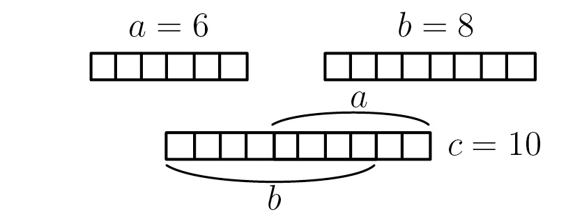
Figure 8. Example of an overlap

We say that the overlap of the maximal length $c=a+b$ is an attachment of $a$ to $b$, and the overlap of the minimal length $c=\max(a,b)$ is an absorption of the smaller number from the pair $a,b$ by the bigger one, Figure 9.

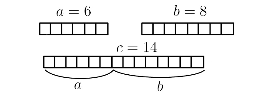
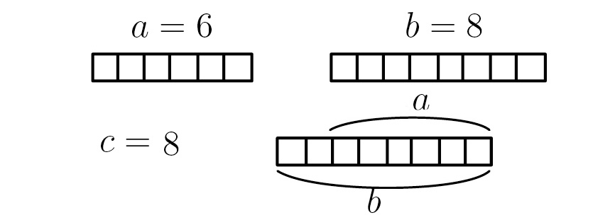
Figure 9. Examples of an attachment and an absorption

Definition 6.4.

Let $\lambda=(\lambda_{1}\geq\dots\geq\lambda_{l})$ and $\mu=(\mu_{1}\geq\dots\geq\mu_{l})$ be two partitions of length $l$. An aggregation of partitions $\lambda$ and $\mu$ is described by the following procedure.

1. Fix a permutation $\sigma$ of the set $\{1,\dots,l\}$.

2. For every $j\in\{1,\dots,l\}$ create an overlap $\tilde{\nu}_{j}$ of parts $\lambda_{j}$ and $\mu_{\sigma(j)}$. One of the overlaps $\tilde{\nu}_{1},\dots,\tilde{\nu}_{l}$ must be necessarily an attachment.

3. Put parts $\tilde{\nu}_{1},\dots,\tilde{\nu}_{l}$ in non-increasing order $\nu_{1},\geq\dots\geq\nu_{l}$. We say that the resulting partition $\nu$ is a result of an aggregation of $\lambda$ and $\mu$ and write
   $[\lambda]+[\mu]\to[\nu]$.

From the discussion of Section 6.1 it is clear that Definitions 6.2 and 6.4 are equivalent.

6.2. Probability distributions of aggregations of partitions.

Transitional probabilities $P_{\lambda,\mu}^{\nu}=P([\lambda]+[\mu]\to[\nu])$ of partitions aggregations can be computed from either definition. Definition 6.2 describes $P_{\lambda,\mu}^{\nu}$ as the number of occurrences of a box $z\in[\nu]$ divided by the total number of all attachments $x$ and $y$ for all $y\in[\mu]$ and a fixed representative $x\in[\lambda]$.

Definition 6.4 equivalently defines $P_{\lambda,\mu}^{\nu}$ as the number of occurrences of partition $\nu$ created by implementing steps (1)-(3) of Definition 6.4 for all permutations of parts of $[\mu]$ and for all overlaps.

Example 6.2.

Tables 4 –7 are examples of probability distributions of partitions aggregations.

$\nu$	[5,2]	[5,1]	[4,3]	[4,2]	[3,3]	[3,2]	otherwise
$P_{[3,1],[2,1]}^{\nu}$	$\frac{2}{14}$	$\frac{1}{14}$	$\frac{2}{14}$	$\frac{4}{14}$	$\frac{3}{14}$	$\frac{2}{14}$	0

Table 4. Results of aggregation $[3,1]+[2,1]$.

$\nu$	[7,3]	[7,2]	[6,3]	[5,5]	[5,4]	[5,3]	[4,3]	otherwise
$P^{\nu}_{[4,2],[3,1]}$	$\frac{1}{10}$	$\frac{1}{10}$	$\frac{1}{10}$	$\frac{1}{10}$	$\frac{3}{10}$	$\frac{2}{10}$	$\frac{1}{10}$	0

Table 5. Results of aggregation $[4,2]+[3,1]$.

$\nu$	[8,3]	[8,2]	[7,3]	[6,5]	[6,4]	[6,3]	[5,5]	[5,4]	[5,3]	[4,3]	otherwise
$P_{[4,2],[4,1]}^{\nu}$	$\frac{2}{22}$	$\frac{2}{22}$	$\frac{2}{22}$	$\frac{2}{22}$	$\frac{4}{22}$	$\frac{2}{22}$	$\frac{2}{22}$	$\frac{3}{22}$	$\frac{2}{22}$	$\frac{1}{22}$	0

Table 6. Results of aggregation $[4,2]+[4,1]$.

$\nu$	[6,2,2]	[6,2,1]	[6,1,1]	[5,2,2]	[5,2,1]	[4,4,2]	[4,4,1]
$P_{[3,1,1],[3,1,1]}^{\nu}$	$\frac{8}{190}$	$\frac{8}{190}$	$\frac{2}{190}$	$\frac{8}{190}$	$\frac{8}{190}$	$\frac{16}{190}$	$\frac{8}{190}$
$\nu$	[4,3,2]	[4,3,1]	[4,2,2]	[4,2,1]	[3,3,2]	[3,2,2]	[3,2,1]	otherwise
$P_{[3,1,1],[3,1,1]}^{\nu}$	$\frac{48}{190}$	$\frac{24}{190}$	$\frac{8}{190}$	$\frac{8}{190}$	$\frac{36}{190}$	$\frac{4}{190}$	$\frac{4}{190}$	0

Table 7. Results of aggregation $[3,1,1]+[3,1,1]$.

6.3. Basic properties of transitional probabilities

Basic properties of probability distribution for aggregation of partitions follow from the definitions.

Proposition 6.1.

1. For any partitions $\lambda,\mu$, $\sum_{\nu}P_{\lambda,\mu}^{\nu}=1$

2. $P_{\lambda,\mu}^{\nu}=P_{\mu,\lambda}^{\nu}$ For any partitions $\lambda,\mu,\nu$,

3. $P^{\lambda,\mu}_{\nu}=0$ if $\nu_{1}\notin[\max(\mu_{1},\lambda_{1}),\mu_{1}+\lambda_{1}]$.

7. Markov chains of self-aggregations

7.1. Repeated self-aggregations

Similarly to Section 5.2, one can consider a Markov chain of repeated aggregations with a fixed partition. In particular, since a unit box $y=(1^{l})$ is invariant under all permutations of coordinates, observations of Section 5.2 can be translated from the model of boxes aggregation to aggregation of partitions in a straightforward way.

In this section we study another class of Markov chains, based on self-aggregations of partitions. This process can be related to monodisperse or hierarchical aggregations, see e.g. [1], [14]. Self-aggregation is an aggregation where a partition aggregates with its own copy. The transition probabilities on the space of partitions of length $l$ are $\{\tilde{p}_{\lambda,\nu}=P_{\lambda,\lambda}^{\nu}\}$. Then the $n$-th step transition probabilities $\{\tilde{p}_{\lambda,\nu}^{(n)}\}$ are defined by recursion rule:

$$\tilde{p}_{\lambda,\nu}^{(0)}=\delta_{\lambda,\nu},\quad\tilde{p}_{\lambda,\nu}^{(1)}=P_{\lambda,\lambda}^{\nu},\quad\tilde{p}_{\lambda,\nu}^{(n)}=\sum_{\mu}\tilde{p}_{\lambda\mu}^{(n-1)}\tilde{p}_{\mu,\nu}^{(1)}.$$

Constructions below are motivated by observations of [7], [12] outlined in Section 2. We aim to trace analytically the presence of mathematical constants $\varphi$ and $\psi$ in two- and three- dimensional growth process (see Section 2). We follow the path of the most frequent transitions of self-aggregations and look at the asymptotical behavior of the proportions of boxes that appear in such sequence. In two-dimensional case our results do involve $\varphi$ in the description of the limiting proportions of the most frequent transitions of self-aggregations. In three-dimensional case our methods do not trace the presence of $\psi$, but further study would be necessary to understand better the behavior of the most frequent transitions in self-aggregation growth.

7.2. The highest probability weight transitions

Definition 7.1.

We say that partition $\nu$ is the aggregation result of two partitions $\lambda$ and $\mu$ with the highest probability weight or is the most frequent transition, if the probability $P_{\lambda,\mu}^{\nu}$ has the maximal value over the set of all possible results of aggregations $[\lambda]+[\mu]\to[\nu]$.

Table 8 provides the highest probability weight aggregation results based on Example 6.2.

Aggregation	The highest probability weight result
$[3,1]+[2,1]$	$[4,2]$
$[4,2]+[4,1]$	$[6,4]$
$[4,2]+[3,1]$	$[5,4]$
$[3,1,1]+[3,1,1]$	$[4,3,2]$
$[\lambda]+[1^{l}]$	$(\lambda_{1}\geq\dots\geq\lambda_{l-1}\geq\lambda_{l}+1>0)$

Table 8. Examples of the highest probability weight results of partitions aggregations

Next we describe the growth along the most frequent transitions in two-dimensional case.

Proposition 7.1.

1. Consider self-aggregation $[\lambda]+[\lambda]\to[\nu]$ of a partition $\lambda=(\lambda_{1},\lambda_{2})$, where $\lambda_{1}>\lambda_{2}+3$. Then the highest probability weight result is $\nu=(\lambda_{1}+\lambda_{2},\lambda_{1})$.

2. Let $\lambda^{(1)}=(\lambda_{1},\lambda_{2})$ with $\lambda_{1}>\lambda_{2}+3$. Consider a sequence of self-aggregations of partitions

   $$[\lambda^{(N)}]+[\lambda^{(N)}]\to[\lambda^{(N+1)}],\quad N=1,2,\dots,\quad$$

   where on each step the highest probability weight result is picked as $\lambda^{(N+1)}$ for the next step of aggregation. Then the shape of the rectangle $\lambda^{(N)}$ tends to the “golden rectangle”:

   $$\lim_{N\to\infty}\frac{\lambda^{(N)}_{1}}{\lambda^{(N)}_{2}}=\varphi=\frac{1+\sqrt{5}}{2}\simeq 1.6180,$$

   and transitional probabilities of the sequence have the limit

   $$\lim_{N\to\infty}P^{\lambda^{(N)}\,\lambda^{(N)}}_{\lambda^{(N+1)}}=\frac{1}{2}-\frac{1}{\varphi+1}\simeq 0.1180,$$

Proof.

1. Let $\nu$ be a result of aggregation $[\lambda]\,+\,[\lambda]\,\to\,[\nu]$. Any rectangle $z\in[\nu]$ is either a result of aggregation $(\lambda_{1},\lambda_{2})+(\lambda_{1},\lambda_{2})\to z$, or $(\lambda_{1},\lambda_{2})+(\lambda_{2},\lambda_{1})\to z$. From Table 3 we get the transitional probabilities for self-aggregation of partitions of two parts, Table 9.

   $\nu$	$P_{\lambda,\lambda}^{\nu}$
   $(2\lambda_{1},2\lambda_{2})$	$\frac{1}{2(\lambda_{1}+\lambda_{2})}$
   $(2\lambda_{1}-s,2\lambda_{2}),\quad s=1,\dots,\lambda_{1}-1$	$\frac{1}{2(\lambda_{1}+\lambda_{2})}$
   $(2\lambda_{1},2\lambda_{2}-s),\quad s=1,\dots,\lambda_{2}-1$	$\frac{1}{2(\lambda_{1}+\lambda_{2})}$
   $(2\lambda_{1},\lambda_{2})$	$\frac{1}{4(\lambda_{1}+\lambda_{2})}$
   $(\lambda_{1},2\lambda_{2})$	$\frac{1}{4(\lambda_{1}+\lambda_{2})}$
   $(\lambda_{1}+\lambda_{2},\lambda_{1}+\lambda_{2})$	$\frac{1}{2(\lambda_{1}+\lambda_{2})}$
   $(\lambda_{1}+\lambda_{2},\lambda_{1}+\lambda_{2}-s),\quad s=1,\dots,\lambda_{2}-1$	$\frac{1}{\lambda_{1}+\lambda_{2}}$
   $(\lambda_{1}+\lambda_{2},\lambda_{1})$	$\frac{\lambda_{1}-\lambda_{2}+1}{2(\lambda_{1}+\lambda_{2})}$
   otherwise	$0$

   Table 9. Probability distribution for self-aggregation of $[\lambda_{1},\lambda_{2}]$.

   It is clear that if $\lambda_{1}-\lambda_{2}>3$, the frequency $P_{\lambda,\lambda}^{(\lambda_{1}+\lambda_{2},\lambda_{1})}=(\lambda_{1}-\lambda_{2}+1)/2(\lambda_{1}+\lambda_{2})$ of the aggregation result $\nu=(\lambda_{1}+\lambda_{2},\lambda_{1})$ is not only the highest value in the table, but it is higher than the sum of frequencies of any other three entries. Hence, even if different values of $s$ produce results of the same sizes, $\nu$ remains to be the most frequent one.

2. Note that ${\lambda^{(N)}_{1}}-{\lambda^{(N)}_{2}}=\lambda^{(N-1)}_{2}>3$ for every $N=2,3,\dots$. Hence, from part (1), by induction on the number of the step, the $N$-th result of the sequence of the most frequent result of self-aggregations has parts

   $${\lambda^{(N)}_{1}}=F_{N}\lambda_{1}+F_{N-1}\lambda_{2},\quad{\lambda^{(N)}_{2}}=F_{N-1}\lambda_{1}+F_{N-2}\lambda_{2},$$

   where $F_{1}=F_{2}=1$, $F_{k+1}=F_{k-1}+F_{k}$ is the Fibonacci sequence. This implies the limit of ratios of sizes and of transitional probabilities:

   $$\lim_{N\to\infty}\frac{\lambda^{(N)}_{1}}{\lambda^{(N)}_{2}}=\lim_{N\to\infty}\frac{F_{N}\lambda_{1}+F_{N-1}\lambda_{2}}{F_{N-1}\lambda_{1}+F_{N-2}\lambda_{2}}=\varphi,$$

   $$\lim_{N\to\infty}P_{\lambda^{(N)}\,\lambda^{(N)}}^{\lambda^{(N+1)}}=\lim_{N\to\infty}\frac{\lambda^{(N)}_{1}/\lambda^{(N)}_{2}-1+1/\lambda^{(N)}_{2}}{2(\lambda^{(N)}_{1}/\lambda^{(N)}_{2}+1)}=\frac{\varphi-1}{2(\varphi+1)}=\frac{1}{2}-\frac{1}{\varphi+1}.$$

∎

Remark 7.1.

From Table 9 observe that $\lim_{N\to\infty}P_{\lambda^{(N)}\,\lambda^{(N)}}^{\nu}=0$ for all other $\nu\neq\lambda^{(N+1)}$.

Example 7.1.

We illustrate Proposition 7.1 with Table 10 of computer-aided calculations of a sequence self-aggregations that starts with $\lambda^{(1)}=[10,6]$ and picks for the next step the highest probability weight result.

$N$	$\lambda^{(N)}$	$\lambda_{1}^{(N)}/\lambda_{2}^{(N)}$	$P_{\lambda^{(N-1)}\,\lambda^{(N-1)}}^{\lambda^{(N)}}$
1	[10, 6]	1.667	$\frac{6}{40}=0.1500$
2	[16, 10]	1.6	$\frac{10}{64}\simeq 0.1563$
3	[26, 16]	1.625	$\frac{14}{104}\simeq 0.1346$
4	[42, 26]	1.6154	$\frac{22}{168}\simeq 0.1310$
5	[68, 42]	1.6190	$\frac{34}{272}=0.1250$
6	[110, 68]	1.6176	$\frac{54}{440}\simeq 0.1227$
7	[178, 110]	1.6182	$\frac{86}{712}\simeq 0.1208$
8	[288, 178]	1.6180	$\frac{138}{1152}\simeq 0.1198$
9	[466, 288]	1.6181	$\frac{222}{1864}\simeq 0.1191$

Table 10. A sequence of highest probability weight self-aggregations.

7.3. The most frequent self-aggregation of three-dimensional partitions

The direct analogy of the results of Section 7.2 in the three-dimensional case that would support interpretations of of [7], [12] would be a stabilization of (almost) any sequence of the most frequent aggregations to a pattern of the form $[\lambda_{1},\lambda_{2},\lambda_{3}]\to[\lambda_{1}+\lambda_{3},\lambda_{1},\lambda_{2}]$. This would lead to natural appearance of $\psi$ in the asymptotical description of proportions of highest probability weight self-aggregations. However, we did not observe such phenomena in general. It seems that in many typical examples after a few steps the process produces not just one, but a family of most frequent results with the same probability weight, as illustrated in Figures  10-12. Moreover, once this process hits a cube $(a,a,a)$ shape, the next step brings a very large number of equally likely most frequent results (Figures  10 and  12).

Thus, tracing the growth of highest probability weight self-aggregations provides an evidence for the proposed in [7, 12] interpretation of the peak of probability distribution of proportions for $l=2$, but does not detect any role of $\psi$ in the description of the peak of probability distribution of proportions for $l=3$. We hope to investigate in more details the typical behavior of the most frequent transitions of self-aggregations for $l\geq 3$ elsewhere.

Figure 10. A sequence of highest probability weight self-aggregation results that starts with $\lambda=[10,3,1]$.

Figure 11. A sequence of highest probability weight self-aggregation results that starts with $\lambda=[3,1,1]$.

Figure 12. A sequence of highest probability weight self-aggregation results that starts with $\lambda=[7,5,3]$.

7.4. Conclusions

We defined two lattice growth models, where clusters are represented by rectangular boxes, that either move without rotations (aggregation of boxes), or can rotate before an attachment (aggregation of partitions). Under assumption of equal probability of attachments at any lattice point of the boundary of the box, we described the set of all possible aggregations and its local statistical characteristics. In particular, we derived the generating function of the moments of the random variable of the number of directions of the growth of an $l$-dimensional box. The combinatorics of these calculations is given by elementary symmetric functions. We also observe that Markov chain of aggregations with a unit box provides a recurrence relation of multidimensional Delannoy numbers with non-constant weights.

In 2-dimensional case we obtained a nice evidence in support of the mathematical interpretation [7, 12] of the peak value point of the distribution of proportions of clusters in DLCA model. We proved that the most frequent transitions in self-aggregations of rectangles stabilize to side-to-end pattern, as in RHM model, and for this reason their proportions grow by Fibonacci-like rule with the limit value $\varphi\simeq 1.618,$. We observed that transitional probability of this sequence tends to $\frac{1}{2}-\frac{1}{\varphi+1}\simeq 0.12$, while transitional probabilities of all other results diminish to zero.

In dimensions $l\geq 3$ the approach of tracing self-aggregations with the highest probability weight does not provide immediate evidence for proposed in [7, 12] interpretation of the peak value of proportions of aggregated clusters. Still, the behavior of sequences of the most frequent transitions of self-aggregations remains an interesting problem that we plan to investigate further.

References

- [1] Botet, R., Jullien, R., and Kolb, M. (1984). Hierarchical Model for Irreversible Kinetic Cluster Formation. J. Phys. A: Math. Gen., 17:L75–L79.
- [2] Caughman, John S.; Dunn, Charles L.; Neudauer, Nancy Ann; Starr, Colin L. Counting lattice chains and Delannoy paths in higher dimensions, Discrete Math. 311 (2011), no.16, 1803–1812.
- [3] Caughman, John S, Haithcock, Clifford R., Veerman, J. J. P. A note on lattice chains and Delannoy numbers Discrete Math.308 (2008), no.12, 2623–2628.
- [4] Chung, Kai Lai Markov chains with stationary transition probabilities Second edition Die Grundlehren der mathematischen Wissenschaften, Band 104 Springer-Verlag New York, Inc., New York, (1967).
- [5] Diaconis, P. Fulton, W. A growth model, a game, an algebra, Lagrange inversion, and characteristic classes. Commutative algebra and algebraic geometry, II (Italian) (Turin, 1990) Rend. Sem. Mat. Univ. Politec. Torino 49 (1991), no.1, 95–119.
- [6] Grau, José María; Oller-Marcén, Antonio M.; Varona, Juan Luis A class of weighted Delannoy numbers, Filomat 36 (2022), no.17, 5985–6007.
- [7] Heinson, W.R., Chakrabarti, A., Sorensen, C.M. Divine proportion shape invariance of diffusion limited cluster-cluster aggregates (2015) Aerosol Science and Technology, 49 (9), pp. 786-792.
- [8] Macdonald, I. G. Symmetric functions and Hall polynomials. Oxf. Class. Texts Phys. Sci. The Clarendon Press, Oxford University Press, New York, (2015).
- [9] Meakiin , P. , Fractals, Scaling, and Growth Far From Equilibrium (Cambridge: Cambridge University Press), (1998).
- [10] Meakin, P. Historical introduction to computer models for fractal aggregates (1999) Journal of Sol-Gel Science and Technology, 15 (2), pp. 97-117.
- [11] Sander, L.M. Diffusion-limited aggregation: A kinetic critical phenomenon? (2000) Contemporary Physics, 41 (4), pp. 203-218.
- [12] Sorensen, C.M., Oh, C. Divine proportion shape preservation and the fractal nature of cluster-cluster aggregates (1998) Physical Review E - Statistical Physics, Plasmas, Fluids, and Related Interdisciplinary Topics, 58 (6), pp. 7545-7548.
- [13] Wang, Yi, Zheng, Sai-Nan, Chen, Xi Analytic aspects of Delannoy numbers, Discrete Math.342 (2019), no.8, 2270–2277.
- [14] Warren, P.B., Ball, R.C. Anisotropy and the approach to scaling in monodisperse reaction-limited cluster-cluster aggregation (1989) J. of Phys A: Math. and Gen., 22 (9), art. no. 027, pp. 1405-1413.
- [15] Witten, T.A., Sander, L.M. Diffusion-limited aggregation, a kinetic critical phenomenon (1981) Physical Review Letters, 47 (19), pp. 1400-1403.
- [16] On Growth and Form Fractal and Non-Fractal Patterns in Physics Editors: H. Eugene Stanley, Nicole Ostrowsky NATO Science Series E: (NSSE, volume 100), (1986).
- [17] Heinson, W.R., Sorensen, C.M., Chakrabarti, A. A three parameter description of the structure of diffusion limited cluster fractal aggregates (2012) Journal of Colloid and Interface Science, 375 (1), pp. 65-69.
- [18] Sorensen, C.M. The Mobility of Fractal Aggregates: A Review, Aerosol Science and Technology, 45:7, 765-779, (2011).