In-Storage Acceleration of Graph-Traversal-Based Approximate Nearest Neighbor Search

Abstract

Approximate nearest neighbor search (ANNS) is a key retrieval technique for vector database and many data center applications, such as person re-identification and recommendation systems. Among all the ANNS algorithms, graph-traversal-based ANNS achieves the highest recall rate. However, as the size of dataset increases, the graph may require hundreds of gigabytes of memory, exceeding the main memory capacity of a single workstation node. Although we can do partitioning and use solid-state drive (SSD) as the backing storage, the limited SSD I/O bandwidth severely degrades the performance of the system. To address this challenge, we present NDSearch, a near-data processing (NDP) solution for ANNS processing. NDSearch consists of a novel in-storage computing architecture, namely, SearSSD, that supports the ANNS kernels and leverages logic unit (LUN)-level parallelism inside the NAND flash chips. NDSearch also includes a processing model that is customized for NDP and cooperates with SearSSD. The processing model enables us to apply a two-level scheduling to improve the data locality and exploit the internal bandwidth in NDSearch, and a speculative searching mechanism to further accelerate the ANNS workload. Our results show that NDSearch improves the throughput by up to 31.7$\times$, 14.6$\times$, 7.4$\times$ 2.9$\times$ over CPU, GPU, a state-of-the-art SmartSSD-only design, and DeepStore, respectively. NDSearch also achieves two orders-of-magnitude higher energy efficiency than CPU and GPU.

I Introduction

Approximate nearest neighbor search (ANNS) is the fundamental retrieval technique of the similarity search in the vector database [1, 2] and an important component in the machine learning (ML) pipeline of many modern data center applications such as recommendation systems [3], image retrieval [4], and person re-identification [5]. In these applications, a query is usually processed by two stages [6, 7]: retrieve/recall stage and rank/identification stage. During the first stage, a fixed number neighbors are retrieved from the database. Then, during the second stage, the retrieved data of the given query is further delicately processed by the specialized models. Instead of getting the exact nearest neighbors, ANNS boosts the search speed by limiting the range of candidates and sacrificing some recall rate. Since the modern vector database and ML applications deal with large-scale data, boosting the performance of ANNS is critical.

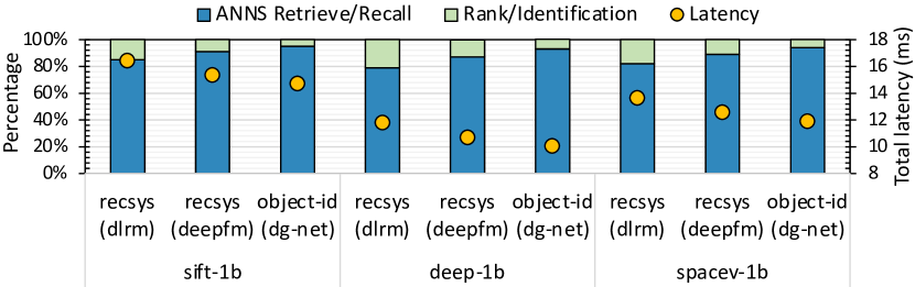
Figure 1: Execution time breakdown and total latency of the two-stage applications: recommendation systems (RecSys) with deep learning recommendation model (DLRM) [8] and deep factorization-machine (DeepFM) [9], and object re-identification (object-reid) with dg-net [7] on Intel Xeon Gold 6245 CPU. 10 candidate vectors are retrieved by ANNS and then processed by respective models. Due to privacy and confidentiality issues, the databases from the industry are not avaliable. This analysis is alternatively conducted on the three public datasets, sift-1 [10], deep-1b[11], and spacev-1b [12]. For RecSys with DLRM, the retrieved vectors are recognized as the embedding vectors in the model while for RecSys with DeepFM and object-reid, the retrieved vectors are recognized as the inputs of the models during the second stage.

As illustrated in Fig. 1, the analysis of the end-to-end execution overhead of the two-stage applications is conducted. Performing ANNS during the retrieve/recall stage averagely takes 87% of the total execution latency, which strongly motivate us to make specialized design to accelerate ANNS workloads.

Among existing methods [13, 14, 15] of ANNS, graph traversal-based methods such as hierarchical navigable small world graphs (HNSW, also the method used in Fig. 1) [16] and DiskANN [17] are the most popular ones for the optimal recall-throughput tradeoff that they achieved [18]. These methods construct a graph based on the distance between the feature vector of each vertex in the dataset. The search is then performed by traversing the neighboring vertices of the visited ones until the predefined condition is met. The graph traversal-based ANNS consists of three steps: graph traversal, distance computation, and bitonic sorting. Graph traversal searches for the potential nearest neighbors of the given queries; distance computation calculates the Euclidean/angular distance between the visited vertices and the queries; and bitonic sorting [19] generates the top-k candidates of each query in a batch.

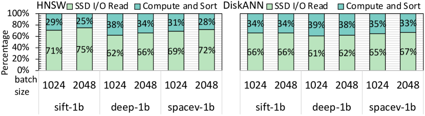
Figure 2: Execution time breakdown of HNSW and DiskANN running on two Intel Xeon Gold 6245 CPUs.

In large-scale real-world applications, a graph can contain up to billions of vertices [20]. Considering the feature vector and the adjacency information associated with each vertex, the workload may consume a significant amount of memory. For example, in HNSW, the memory consumption per vertex ranges from 60 bytes to 450 bytes [21]. Given the large number of vertices, the required memory of ANNS could reach hundreds of gigabytes (GBs) or even several terabytes (TBs), which exceeds the total capacity of the main memory on a single node in the workstation [22].

Existing solutions generally adopt three approaches to fulfill the memory capacity demand: (i) sharding the dataset, storing the shards in the disk, loading a limited number of shards into memory, and only routing the query to these shards to perform the search locally [23]; (ii) developing programs with SSD-based indices to fetch the feature vectors from SSD into the main memory at runtime [22]; (iii) loading the whole dataset from the SSD into multiple nodes’ main memory at the cost of expensive machines and high power consumption, e.g., accelerating ANNS with 8 A100 GPUs [24]. Although these designs can support graph-traversal-based ANNS on very large datasets, their performance is greatly limited by the SSD I/O read (the time taken by data transfer via PCIe) in terms of the end-to-end performance, as shown in Fig.2. The SSD I/O read accounts for up to 75% of the total latency. From Fig.3(a), we can see that the utilization of SSD I/O bandwidth saturates to 83%, after the batch size increases to 1024. Combined with Fig. 2, the saturated SSD I/O bandwidth illustrates that the SSD I/O read latency comes from the limited I/O bandwidth. In the current computer systems, CPU and SSD are usually connected via PCIe links, e.g., PCIe 3.0 $\times$ 16 whose peak bandwidth is about 15.4 GB/s. Fig. 3(b) further shows that the ANNS workloads are located in the SSD I/O bandwidth-constrained region. We conclude that the SSD I/O bandwidth limits the performance of ANNS. To fundamentally address the issue, we envision that a promising solution is to directly process the large-scale ANNS workload within the storage.

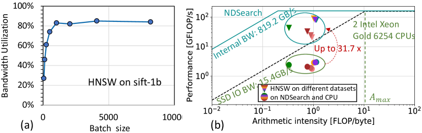
Figure 3: (a) PCIe bandwidth saturates as the batch size increases; (b) Roofline lifting effect and the ANNS workloads speedup enabled by NDSearch (all the page buffers can be read simultaneously). The (color,shape) tuples represent different ANNS workloads, i.e., HNSW on different datasets.

However, it is not straightforward to implement graph traversal-based ANNS within the storage devices. From the hardware side, current in-storage accelerators like DeepStore [25] are unable to fully utilize the internal SSD bandwidth for graph traversal-based ANNS because ANNS’s irregular and sparse data access pattern require more fine-grained level parallelism. From the software side, current processing models of graph traversal [26, 27] lacks the applicability to the in-storage architectures, especially the customized dataflow and scheduling. To tackle the above challenges, we propose NDSearch, an NDP solution for ANNS based on SmartSSD [28]. The operations of the graph traversal and distance computation kernels are offloaded to the SSD. We studied the data access pattern of graph traversal on SSDs and found that the fine-grained and in-place acceleration at the logic unit (LUN) level is the most promising solution for processing the irregular and scattered accesses to feature vectors in graph-traversal-based ANNS. Hence, we develop LUN-level accelerators on flash chips with the modified multi-LUN operations. Meanwhile, the high parallel bitonic sorting is offloaded onto the FPGA like  [29] to allow more power and area budget. To fully exploit the proposed architecture, NDSearch also includes a novel processing model designed for ANNS in NDP scenarios. The processing model is based on GraphMat [26] and incorporates a two-level scheduling scheme, static and dynamic scheduling. Static scheduling reorders and maps the vertices to the physical location with the goal of enabling multi-plane operations and maximizing the spatial locality. Based on a new graph format, LUNCSR, dynamic scheduling aims at maximizing the temporal locality of the data by allocating the queries based on the location of the required data. A speculative searching mechanism is integrated into the dynamic scheduling to prefetch the vertices.

Our contribution can be summarized as follows.

• We conduct a characterization study on graph-traversal-based ANNS and identify the opportunities of offloading the graph traversal and distance computation kernels to SSDs to address the issues of large memory consumption and limited SSD I/O bandwidth.

• We propose an NDP architecture design and a corresponding processing model to support graph-traversal-based ANNS.

• We develop a two-level scheduling scheme to both reorder the vertices in the SSD and dynamically allocate and prefetch queries during the search based on a new graph format, namely, LUNCSR.

The experimental results show up to 14.6$\times$ and 2.9$\times$ speedup over GPU and DeepStore, respectively. NDSearch also achieves up to 30.06 $\times$ and 3.48 $\times$ higher energy efficiency than a state-of-art SmartSSD design [30] and DeepStore [25].

II Background

II-A Graph-traversal-based ANNS

ANNS is an approximation to the original nearest neighbor search (NNS) algorithm [31], which aims to find top-K elements to a given query with minimized distances by scanning the whole dataset. Due to the high search cost of the brute-force search in NNS, ANNS is selected as an alternative and faster approach in scenarios where a lower recall rate is acceptable. Recently, graph-traversal-based ANNS such as HNSW [16] and DiskANN [17] become popular due to their superior performance in the real life applications. Although the details of these two algorithms are different, the common basics can be generally summarized as follows.

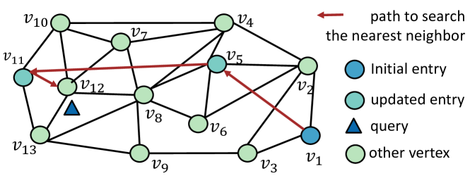
Figure 4: The search phase of graph-traversal-based ANNS.

Graph-traversal-based ANNS consists of two phases, construction and search. In the construction phase, a graph is constructed based on raw feature vectors in the dataset. Firstly, a distance function is defined to characterize the similarity between two vectors. Then, given a distance threshold and the maximum number of neighbors that one vector can have, incoming vectors are consecutively inserted in random entries and bidirectionally connected to their neighbors. Finally, vectors are built as vertices in the constructed graph. Each vertex consists of its feature vector and adjacency information (i.e., which neighbors the vertex is connected to and the distances between the vertex and the neighbors). In the search phase, for a given query, a random entry vertex is firstly selected and put into the candidate list. Then the nearest vertex $C$ to the query is selected as the updated entry vertex from all the candidates and removed from the candidate list. If the distance between $C$ and the query meets a pre-defined condition or is far greater than a marked value in the result list, where the distances between the visited vertices and the query are stored, then the searching is terminated. Otherwise, add the neighbors (which are never visited) of $C$ to the candidate list. After traversing all the vertices in the candidate list and repeating the process above, the final top-K vertices from the results list are selected and sorted according to the distances in ascending order. Fig. 4 shows a naïve example of searching the approximate nearest neighbor of the query. Our work mainly focuses on accelerating the search phase of ANNS, which is directly applied to various applications, and leaves the construction phase to future work.

II-B SSD Preliminary

II-B1 Internal organization

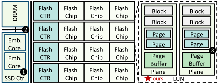
Figure 5: SSD internal organization and architecture changes of prior in-storage computing works and ours.

As illustrated in Fig. 5 modern SSD consists of 2–4 embedded cores as the SSD controller, a few GBs of DRAM, and 16–32 channels of flash chips as the storage [32]. The NAND flash storage elements are hierarchically organized at multiple levels - channels, chips, logic units (LUN), planes, blocks, and pages. Each channel contains a flash controller and 4–8 flash chips, each of which includes 2–8 planes. Each plane is made of a group of blocks and a page buffer. Each block has multiple pages, whose size could be 2/4/8/16 KB. One or more planes are organized as a LUN [33, 34], which is the minimal unit that can independently execute commands. Multi-LUN [35, 34] operations are supported in the flash chip to improve the in-chip parallelism. Multi-plane operations can be supported to maximize the operation parallelism in a LUN. The address of NAND flash consists of two parts: the column address and the row address [36]. The column address is used to access bytes or words within a page, while the row address is used to address pages, blocks, and LUNs.

II-B2 Data refreshing and address translation

The flash transaction layer (FTL) runs on the embedded cores to process data refreshing, address translation, garbage collection and etc [37]. Although the search phase of ANNS on NDSearch does not induce graph updates and only operates in a read-only mode, the NAND flash requires data refreshing and data correction due to retention and read disturbance issues, resulting in the flash addresses being changed. We employ the block-level FTL refreshing mechanism and integrate the logical-to-physical address translation in the design of LUNCSR (see Section IV-B for the details). We use the specialized hardware component to infer the final physical address with the vertex index to eliminate the overhead of executing FTL address translation on the embedded cores. Compared to DeepStore [25] which just considers the change of the starting address of the database, our design is more realistic in terms of data refreshing and address translation.

II-C Related works about in-storage computing

In-storage computing architectures aim to offload the data-intensive workloads to the storage devices like SSD to reduce the expensive data movement from and to storage. Modifying the internal architecture of SSD is required to develop an in-storage accelerator. Three categories of in-storage computing architectures have been proposed (as marked in Fig. 5): ❶ modifying the firmware of the SSD controller (embedded cores) [38, 39]; ❷ adding customized hardware modules inside the SSD without touching the NAND flash chips [40, 41, 25, 42, 43]; ❸ changing the internal architecture of NAND flash chips, e.g., adjusting the latching circuit or adding the digital logic in flash memory [44, 45, 46]. Choosing the way to modify the SSD architecture depends on the requirement of the data access pattern and the arithmetic intensity of the specific workload. According to the characteristics of the ANNS workloads (see Section III), we develop LUN-level accelerators in flash chips. Differing from the prior works which utilize the SSD internal bandwidth through simultaneous accesses to different flash channels, our work further improves the bandwidth of each flash channel by the modified multi-LUN operations that exploit both the temporal and spatial data locality in all the page buffers, as shown in Fig. 3(b). Meanwhile, the data movement from flash channels is also reduced within the SSD.

III Motivation

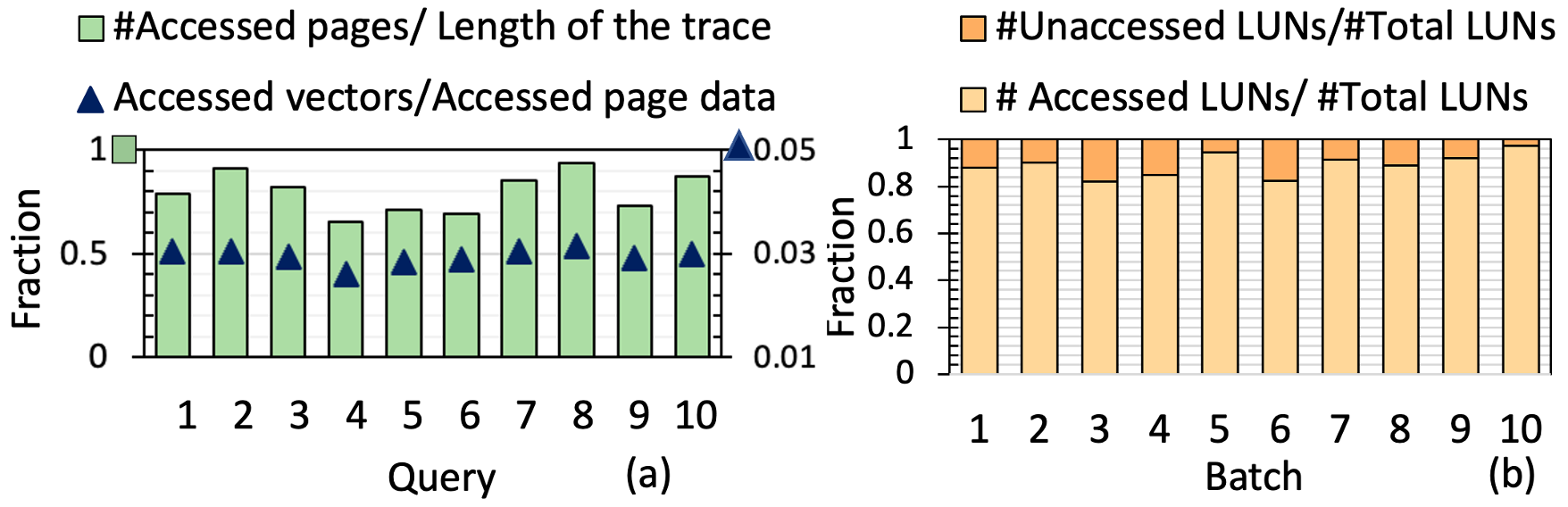
Figure 6: Page and LUN access pattern of the search phase.

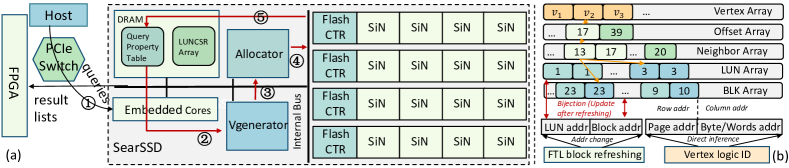
Figure 7: (a) Overview of NDSearch and overall architecture of SearSSD; (b) The new graph format - LUNCSR with LUN and BLK array.

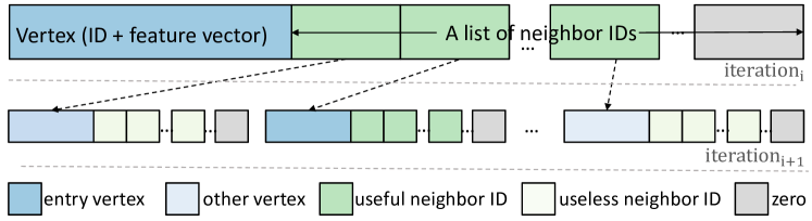
Figure 8: The inefficient data layout in NDP scenarios.

Reordering and remapping vertices to improve spatial data locality in the page buffer. We studied the behavior for the query-wise and batch-wise search of ANNS at different levels of SSD organization. Fig. 6 (a) illustrates the ratio of the number of page accesses to the length of the searching trace (the number of visited vertices that are computed with the given query), and the ratio of the size of accessed feature vectors to the size of accessed page data of 10 random sampled queries in a batch. The high #Accessed pages/#Length of the trace ratio and low Accessed vectors/Accessed page data ratio indicate that the fine-grained accesses to vertices are scattered among different pages, which means that the page buffer locality is very poor and the access pattern is irregular in the search if the vertices were stored in the order the graph was constructed. This motivates us to reorder the graph vertices and then remap the data to improve spatial data locality in the page buffer, and thus reduce the number of accesses to pagesfor each query in the search phase.

Developing LUN-level accelerators and dynamic scheduling to improve temporal data locality within one batch. As shown in Fig. 6 (b), during the search of 10 consecutive batches (with batch size set to 2048) of queries in sift-1b dataset, over 82% of all the LUNs that store the vertices are accessed in each batch (The vertices are stored in the order of graph construction). This indicates that the pattern of access to LUNs is highly scattered, and it is possible to explore the LUN-level parallelism and internal bandwidth to speed up the execution. In addition, according to inclusion-exclusion principle [47], there must be multiple accesses to one LUN when the batch size is larger than the number of total LUNs. In the original SSD architecture, since the data bus is shared by multiple LUNs, only one LUN of one flash chip in a specific channel can be selected to occupy the bus, thus adopting SSD/channel/chip-level accelerators like  [25] hinders the operational parallelism. Moreover, reading data from the page buffer to the accelerators outside the NAND Flash chip induces extra $\sim 30\mu s$ latency. Hence, based on these observations, we (i) develop LUN-level accelerators based on the existing multi-LUN operations to explore the internal operation parallelism of NAND Flash; and (ii) propose a dynamic scheduling mechanism to allocate the queries, whose targeted vertices are in the same LUN, in one batch to the same LUN based on our LUNCSR graph format, to improve the temporal data locality.

IV NDSearch Architecture

IV-A Architecture overview

This section presents NDSearch, a system that accelerates graph-traversal-based ANNS by leveraging the computational storage device based on SmartSSD [28] architecture. Fig. 7(a) illustrates the overview of NDSearch, which consists of an FPGA device and a modified SSD device connected by a private PCIe 3.0$\times$4 link. As aforementioned, we extract three kernels from the workload of graph-traversal-based ANNS, graph traversal, distance computation, and bitonic sorting. We modify the original SSD as SearSSD and offload the graph traversal and distance computation kernels to it. The graph traversal kernel is executed in the embedded cores with additional customized logic (Vgenerator and Allocator) in the SSD. The distance kernel runs on the Search-in-Nand (SiN) engines where LUN-level accelerators are developed. Each SSD channel consists of four SiN engines. SearSSD outputs the result lists of each query to the FPGA. The result list of one query only needs to contain the index of the query, the indices of the query’s candidate neighbors, and the scalar distances between the query and the candidates. The feature vectors of query and targeted vertices are “filtered” by the SearSSD to reduce the PCIe bandwidth consumption, which could be as low as $1/32$ of the data transferred via PCIe link in [30]. The FPGA executes the bitonic sorting kernel and returns the top-k neighbors of each query to the host.

IV-B Data layout – LUNCSR

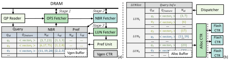
Figure 9: The detailed architecture of (a) Vgenerator and (b) Allocator.

DiskANN [17] and HNSW [16] adopt the same data layout such that for each vertex $i$, the feature vector $v_{i}$ before the IDs of its $\leq R$ (i.e., $R=32$) neighbors and zeros are padded if the degree of a node is smaller than $R$, as shown in Fig. 8. We argue that this data layout is inefficient for NDP solutions for two reasons. First, it wastes space by padding zeros to align the feature vectors and neighbor IDs. Second, it fetches unnecessary neighbor IDs that are not used in the search process. For example, suppose each vertex has a 128-byte feature vector and 32 4-byte neighbor IDs, resulting in a 256-byte slice of data layout. Then, 16 such slices can fit in one page (assume 4KB page size), which is the minimal access granularity in the NAND array. However, during the search, only the neighbor IDs of the closest vertex to the query in each iteration are needed for the next iteration. The rest of the neighbor IDs in the page are irrelevant and cause at least 46.9% storage overhead as shown in Fig. 8. Notice that this data layout is efficient if the graph is stored in DRAM or GPU memory, where the access granularity is the cacheline size - 64 bytes, because the smaller granularity decouples the accesses to the feature vectors and neighbor IDs, i.e., accessing the 128-byte feature vector just requires two memory reads without loading neighbor IDs. In addition, the smaller granularity also induces less access to the irrelevant neighbor IDs. Hence, we found that the compressed sparse row (CSR) is more suitable for the NDP solution since the vertex and neighbor IDs are separately stored. We can avoid accessing data that will not be used by the subsequent process under the same page access.

CSR is widely used as an efficient format to store graphs. The original CSR format consists of three one-dimensional arrays: offset, neighbor, and vertex arrays [48]. The original CSR format does not encode the vertex placement information, which could be critical for NDP. Thus, we propose LUNCSR, which extends the CSR format by adding two additional arrays, LUN array and block (BLK) array. The LUN array stores the physical LUN allocation of the vertices, and the BLK array stores each vertex’s relative physical block allocation within a LUN. Both arrays can be indexed by the vertex IDs or the neighbor IDs and updated by FTL when data refreshing occurs. As discussed in Section II-B2, NDSearch uses block-level refreshing. Fig.7(b) shows how FTL updates the LUN and BLK arrays when the block-level refreshing changes the LUN and block addresses. The LUN and BLK arrays are managed in a similar way that FTL manages the mapping table in the traditional SSDs to guarantee the coherency and consistency of the data. After confirming that no data refreshing happens or the infrequent data refreshing has been done, the specialized Allocator finally generates the physical address of a vertex according to its logical index and the LUNCSR without adopting FTL to do the logical-to-physical address translation. The page/column address can be directly inferred from the logical index of a vertex since it is not affected by the block-level refreshing. Note that there is no additional memory resources for LUNCSR arrays compared to the standard SSD, where there exists a mapping table for the logical-to-physical address translation. We just transform the mapping table to LUNCSR arrays which can be integrated to NDSearch. Fig. 7(b) also demonstrates how the Allocator indexes the neighbors of $v_{2}$ in the LUNCSR. The arrows illustrate the indexing traces. Specifically, the ID (i.e., 2) of $v_{2}$ points to its first neighbor $v_{13}$ with offset 17. The Allocator uses the offset value as the pointer to access the neighbor list of $v_{2}$ (the length of the neighbor list is the difference between $v_{3}$’s offset and $v_{2}$’s offset). Then, using the neighbor IDs, the Allocator can find the neighbors’ corresponding LUN and block IDs. The neighbor IDs (also the vertex logic IDs in Fig. 7(b)) further indicate the page and column addresses so the physical addresses of each neighbor are finally generated.

IV-C SearSSD design

Fig. 7(a) depicts the overall architecture of SearSSD. The Allocator and Vgenerator are physically implemented on the same die and connected to the internal memory bus of the SSD controller (embedded cores). Only the vertex array in LUNCSR is stored in SiNs. The other arrays are buffered in the internal DRAM or stored in normal NAND flash chips in standard SSD channels which are not illustrated in Fig. 7 (a). To support billion-scale ANNS benchmarks, we set the total capacity of SiNs to 512 GB, organized as 32 channels, 4 flash chips per channel, 4 planes per chip, 512 blocks per plane, and 128 pages per block. The page size is 16KB, and we organize two planes as a LUN. Other detailed configurations of NDSearch are shown in Table II.

IV-C1 Dataflow in SearSSD

The dataflow in SearSSD is also shown in Fig. 7(a). A batch of queries is sent from the host to the SSD controller via the PCIe link. The SSD controller then assigns the initial entry vertex for each query. A query property table is created in the internal DRAM to store the property of each query (i.e., current searching status, including the ID of the query, the ID of entry vertex in this iteration, the feature vectors of the query, result list and etc.) and maintained by the SSD controller. Vgenerator manages to read out the graph information of the entry vertex in LUNCSR format, including offset, LUN IDs, and neighbor IDs. The exact neighbor and LUN IDs are generated in Vgenerator and sent to Allocator. According to the neighbor and LUN IDs from Vgenerator, Allocator allocates the queries and neighbor IDs to different LUNs. Allocator sends the queries and physical addresses of the neighbors (candidates) to the corresponding LUN-level accelerators. The SiN engines compute the distance between the queries and the vertices stored in the NAND flash chips. The computed distances are sent back to the SSD controller to update the query property table. A new vertex is selected as the updated entry vertex of the next search iteration. The loop of repeats until the search of the batch of queries terminates.

IV-C2 Vgenerator

The architecture of the Vgenerator is depicted in Fig. 9(a). The Vgen Buffer is partitioned into three portions: Query, neighbor (NBR), and prefetch (Pref) buffers. A batch of queries are written into the query buffer. Then the QP reader reads the IDs of entry vertices in the current search iteration and sends them to OFS Fetcher. OFS Fetcher, NBR Fetcher, and LUN Fetcher work in a three-stage pipeline to fetch the offset values, the neighbor IDs, and the LUN IDs of the neighbors of the entry vertices, respectively, following the indexing process which is described in Section  IV-B. Then the NBR Fetcher writes the neighbor IDs into the “$N_{id}$” fraction of the NBR buffer while LUN Fetcher writes the corresponding LUN IDs into “$L_{id}$” fraction of the NBR buffer. The Pref Unit is used to prefetch the neighbors to do the speculative searching, which will be introduced in detail in Section VI.

IV-C3 Allocator

The architecture of the allocator is illustrated in Fig. 9(b). According to the $L_{id}$ in the Vgen Buffer, the Dispatcher gathers the neighbors with the same LUN IDs and the corresponding queries together in the same fraction of Alloc Buffer, which is horizontally partitioned according to LUN IDs. Then, the Alloc CTR directly generates the physical addresses of all the neighbors using the $N_{id}$s and the corresponding content in LUN/BLK array as described in Section IV-B, avoiding the FTL address translation overhead. Next, the Alloc CTR sends the data and the physical addresses to the corresponding LUN-level accelerator through Flash CTR for distance computation.

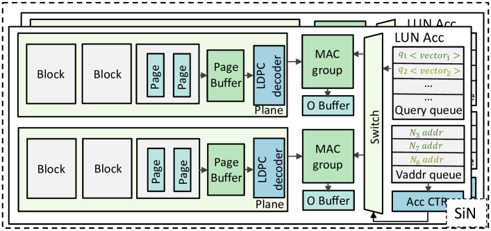
Figure 10: The architecture of SiN including two LUN accelerators.

IV-C4 SiN

Fig. 10 shows the architecture of the SiN engine whose basic unit is an LUN-level accelerator. One SiN is made up of 2 LUN-level accelerators. The Flash CTR sends the modified multi-LUN instructions to the SiN to make the LUN-level accelerators in the same SiN process the queries in parallel. In each LUN-level accelerator, the query queue buffers the feature vectors of queries that are allocated to this LUN, and the Vaddr queue buffers the addresses for the neighbors of each query in the current search iteration. The Acc CTR sends multi-plane instructions to read vertices from different planes and enables the two multiply-and-accumulate (MAC) groups to work in parallel. The queries are sent to the corresponding MAC group via a switch. The computed distances are temporarily stored in the additional output buffer (O Buffer) for readout. Under the premise of 256 LUN-level accelerators in total, we build 2 MACs into each MAC group, whose architecture is based on the adder tree and similar to the design in  [30]. The feasibility of the MAC group and its influence on the storage density is discussed in Section VII-B.

IV-C5 ECC mechanism in SiN

Error correction code (ECC) [49] mechanism is indispensable in SSD, which is used to detect and correct data error induced by the noise and distortion of NAND flash memory cells. We develop the plane-level ECC mechanism in SiN because we should make sure that the accessed feature vectors are corrected before being fed into the MAC group. Hence, as shown in Fig. 10, a hard-decision decoder [50] is put between the page buffer and the MAC group in each plane. We adopt low-density parity-check (LDPC) [51] codes for ECC, which are initially written into NAND flash memory along with feature vectors. Soft-decision [52] LDPC decoding still runs on the FTL layer on the embedded cores and is invoked only if the hard-decision decoding fails. In most cases, implementing hard-decision decoders in SiN is sufficient for the search phase of ANNS. The corresponding evaluation is shown in Section VII-B .

IV-C6 Multi-LUN operation modification

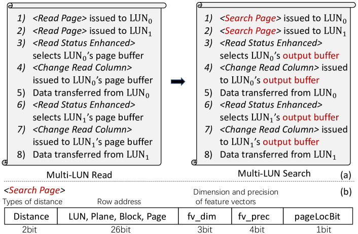
Figure 11: (a) The modified workflow of multi-LUN operation; (b) The instruction of search page.

Our multi-LUN search operation is based on the existing multi-LUN read operation in SSD. The typical workflow of multi-LUN read is shown at the left of Fig. 11(a). We change the $<ReadPage>$ instruction to the specialized $<SearchPage>$ instruction, which is illustrated in Fig. 11(b). The 2-bit “Distance” portion indicates which type of distance to compute, like Euclidean distance, angular distance, inner-product distance, and so on. We use 1-bit “pageLocBit” to illustrate the locality of the page buffer. If “pageLocBit = 1”, there will be two or more queries’ candidates located on the selected page. In addition, we change the objects of $<ReadStatusEnhanced>$ and $<ChangeReadColumn>$ from the page buffer to the output buffer in our design because we only need to transfer the computed distances from each LUN rather than the original feature vectors. The modified workflow of multi-LUN search is shown at the right of Fig. 11(a).

V Processing model

Current graph traversal-based ANNS follows the widely adopted processing model in graph analytic [26], which consists of two phases - Scatter and Apply, with three essential operators - Processing Edge, Reduce and Apply. We found that it is inefficient for NDSearch since it does not consider the dataflow of graph-traversal-based ANNS or the characteristics of the NDP platform. Thus, we propose a new processing model of accelerating graph-traversal-based ANNS on NDSearch as shown in Algorithm 1. To exploit the parallelism of NDSearch, the model iterate over the LUN list which can be executed in parallel. To overlap the latency of the dynamic scheduling of graph traversal kernel and the execution of distance computation kernel, we decouple the Scatter phase into Allocating and Searching stages, which will be further discussed in Section VI-B2. We also decouple the Apply phase into Gathering and Sorting stages.

Algorithm 1 ANNS Near Data Processing Model

1:  for i in range (len(this batch)) do

2:     $q_{i}.Lid\leftarrow$ Vgenerate ($q_{i}.Prop$)

3:  LUNlist $\leftarrow$ Batch-wise dynamic allocating (this batch) 

4:  while  Searching of this batch is not terminated do

5:     for j in range (len($\#LUNlist$)) do

6:        for i in range (len($LUNlist[j].Q_{id}[i]$)) do

7:           for k in range (len($LUNlist[j].q_{i}.Nid$)) do

8:              ProResult $\leftarrow$ Process Edge ($LUNlist[j].q_{i}$, $v_{LUNlist[j].q_{i}.Nid[k]}$)

9:           $q_{i}.tProp$ $\leftarrow$ Reduce ($q_{i}.Prop$, ProResult)

10:     for i in range (len(this batch)) do

11:        $q_{i}.Prop$ $\leftarrow$ Apply ($q_{i}.tProp$)

12:  return  $q_{i}.top-k$ $\leftarrow$ BitonicSort(for i in range (len(this batch)))

Allocating stage in Scatter phase (line 1$\sim$3): According to the property of each query in the batch, an LUN look-up table is generated and the tasks of the search of queries are allocated to the LUN-level accelerators through the batch-wise dynamic allocating method (See Section VI-B).

Searching stage in Scatter phase (line 4$\sim$8): In the Searching stage, separate LUNs work simultaneously with the support of multi-LUN operations. Process Edge operator executes the distance computation. Reduce operator updates the temporary property of each query, e.g., the result list in the current search iteration. The condition of termination of this stage is determined by the setting in the specific ANNS algorithm.

Gathering stage in Apply phase (line 9$\sim$10): After the Searching stage, the properties of each query in the batch are updated in the Query Property Table by the Apply operator. According to the updated results, the queries that do not meet the termination condition will start the next search iteration which consists of the three stages above.

Sorting stage in Apply phase (line 11): When all queries have met the termination condition, a batch of results lists is sent to the FPGA for sorting. Meanwhile, the allocating stage for the next batch can start. The top-K nearest neighbors of each query will be selected and sent back to the host.

VI Two-level Scheduling

The scheduling in NDSearch involves two levels—static scheduling and dynamic scheduling. The static scheduling reorders the vertices offline for a better spatial locality. Dynamic scheduling processes the graph traverse of a batch of queries at runtime.

VI-A Static scheduling

Before reordering the graph, the vertices in the graph are stored according to the constructing order, which is usually random. The random order of storing the vertices induces poor data locality because the topology information is not captured. Prior methods [53] are either inefficient for breadth-first traversal or incur unacceptable overhead to find a relative good vertices order. Moreover, no prior works consider how to delicately map the reordered data onto the storage devices according to their unique characteristics. Considering the breadth-first traversal trace in the graph traversal-based ANNS algorithms, we propose our degree ascending breadth-first reordering method based on  [54], which only requires running once but can achieve near-optimal performance. We would like to store the neighboring vertices in the graph to the same page in the SSD, to ensure the data locality of page access. However, naïvely mapping the reordered vertices to the consecutive physical addresses in NAND flash will sacrifice the multi-plane parallelism. Hence, after reordering, the mapping of the vertices should be coordinated with the restrictions of multi-plane operations of SSD.

VI-A1 Degree ascending breadth-first traversal reordering

Let $\mathcal{V}=\{v_{1},...,v_{n}\}$ be the $n$ vertices of a graph $G=(\mathcal{V,E})$ with $|\mathcal{E}|$ edges, and $f:\mathcal{V}\to\{1,2,...,n\}$ be a reordering function that generate an index for each vertex of the graph. The goal of the reordering is to find an optimal $f$ to minimize a bandwidth function $\beta(G,f)$ defined as:

$$\beta(G,f)=\frac{1}{n}\sum_{v\in\mathcal{V}}\mathop{max}\limits_{(i,j)\in\mathcal{E}(v)}|f(i)-f(j)|.$$ (1)

Here, $v$ is each vertex in the graph, and $\mathcal{E}(v)$ generates the indices of all the neighbors of the vertex $v$. Our objective is to minimize the average vertex bandwidth, $\beta$. A small $\beta$ guarantees that the neighbors of each vertex are stored physically close to each other. Reordering graph vertices to get the minimum $\beta$ has been proved to be an NP-Completeness problem [55]. Although some prior reordering methods are proposed[56], the existing randomness in these methods requires running the methods multiple times to approach the optimal reordering result. For the example shown in Fig. 12, if using the prior method in [54], there are 8 choices to select $v_{0}$ in the original graph. Furthermore, if $v_{d}$ is selected as $v_{0}$, there are $5!=120$ choices to renumber $v_{a},v_{c},v_{e},v_{f},v_{g}$ to $v_{1}-v_{5}$ . As the reordering proceeds, the reordering results increase significantly and we should finally select one whose $\beta$ is the smallest. The overhead of traversing all the possible BFS orders is unacceptable for the huge scale ANNS graphs.

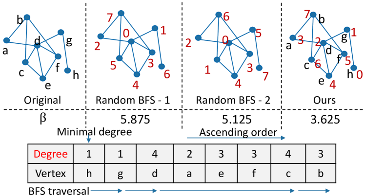
Figure 12: An example of the comparison between random BFS reordering method and our method.

Our reordering method addresses the aforementioned issue of randomness. Specifically, we reorder the vertices based on their degrees in ascending order, which is a deterministic approach rather than a random one. This ordering strategy is motivated by the observation that first randomly labeling the vertices with higher degree (more neighbors) creates difficulty for closely labeling their neighbors (making the indices of the neighbors as close as possible) later, which finally results in a large bandwidth $\beta$. In contrast, if vertices with lower degrees are reordered first, their neighbors with higher degrees may still remain unnumbered and be easy to be closely labeled, resulting in a smaller $\beta$. In addition, by reordering the vertices with higher degrees later in the process, we can reduce $\beta$ further by placing them closer to their already renumbered neighbors. As a result, our method only needs to be run once to obtain a near-optimal vertex reordering, as illustrated in the final reordered graph in Figure 12. Firstly, we select $v_{h}$ which has the minimal degree - 1, as the root vertex $v_{0}$. Then, the BFS traversal would find $v_{g}$, and we renumber it to $v_{1}$. After renumbering $v_{d}$ to $v_{2}$, we reorder its neighbors according to their degree ascending order. In this example, the degrees of $v_{a}$, $v_{c}$, $v_{e}$,$v_{f}$ and $v_{g}$, are 3, 4, 3, 3 and 1, respectively. Because $v_{g}$ has been renumbered, we further renumber $v_{a}$ as $v_{3}$, $v_{e}$ as $v_{4}$, $v_{f}$ as $v_{5}$ and $v_{c}$ as $v_{6}$. The reordering process will continue until all vertices are renumbered. Obviously, there is no randomness existing in our method only if the degrees of some neighbors of a vertex are same. Moreover, this example shows that our method can ensure smaller average bandwidth of each vertex by reducing the opportunities that the neighbors are split far away from each other.

VI-A2 Multi-plane operation

To exploit the parallelism of multi-plane operations, we should map the reordered vertices under the restrictions of multi-plane addressing. There are two restrictions applied to the multi-plane address when executing a multi-plane command sequence on a particular LUN: (i) The plane address bits shall be distinct from any other multi-plane operation in the multi-plane command sequence; (ii) The page/LUN address shall be the same as any other multi-plane operations in the multi-plane command sequence. Hence, our mapping strategy is that we first map the reordered vertices in one page of a plane to one LUN, e.g., $page_{i}$ in $plane_{j}$, to maximize the data locality in one page. Then, we choose the same $page_{i}$ in another $plane_{j+1}$ in the same LUN. Next, we iteratively perform the mapping with the aforementioned process on different LUNs. If we have selected all LUNs, we go back to the first LUN and select a different page number for the subsequent vertices. As illustrated in Fig. 13, the arrow shows the path of mapping.

In addition, we also consider the the influence of data refreshing on our static scheduling. As aforementioned, we adopt block-level data refreshing in SearSSD. Obviously, our degree ascending breadth-first traversal reordering is not affected because we reorder the vertices to improve the page-level data locality. To avoid degrading the parallelism of multi-plane operation, which is achieved by our mapping strategy, we make the block-level data refreshing happen within planes instead of arbitrary locations in the SSD.

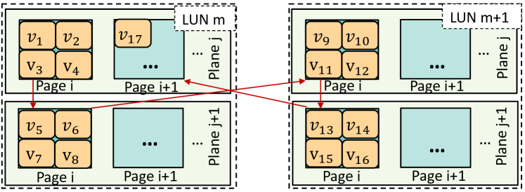
Figure 13: Mapping of vertices restricted by multi-plane addressing.

VI-B Dynamic scheduling

Our dynamic scheduling, which is executed by Vgenerator and Allocator, aims to efficiently allocate queries to the corresponding LUN-level accelerators to improve temporal data locality in each LUN and overlap the latency between search iterations within one batch of queries. It consists of batch-wise dynamic allocating and speculative searching.

VI-B1 Batch-wise dynamic allocating

This technique allocates queries with the same targeted LUNs to the corresponding LUN-level accelerators at once. The implementation of the batch-wise dynamic allocating is suggested in the architecture design of Vgenerator and Allocator in Section IV-C2 and Section IV-C3 An example is illustrated in Fig. 9, where $q_{1}$ is sent to $LUN_{1}$ and $LUN_{3}$, $q_{2}$ is sent to $LUN_{1}$ and $LUN_{2}$, and $q_{3}$ is sent to $LUN_{2}$ and $LUN_{3}$ to be computed distances with the corresponding neighbors. Note that one query can be allocated to different LUN-level accelerators. The allocated queries in each LUN are further assigned to the corresponding planes in a similar way to allocating queries to LUNs. In this way, the pages consisting of the candidate neighbors of different queries only need to be loaded once from the plane and the temporal data locality in each LUN is fully exploited.

VI-B2 Speculative searching

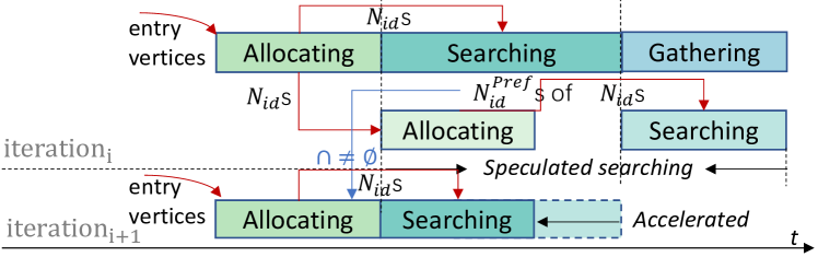
Figure 14: The mechanism of speculative searching.

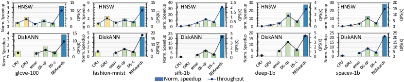
Figure 15: Speedup normalized to CPU (shown in the histogram) and throughput (shown in the line chart) comparison on various platforms. We measure the throughput by processing a batch (2048) of queries with the same memory trace on each benchmark.

As aforementioned in Section V, a common search iteration consists of three sequential stages: Allocating stage, Searching stage, and Gathering stage as illustrated in Fig. 14. The Allocating stage of the next search iteration usually requires the updated results of Gathering stage of the current iteration (iteration_i in Fig. 14) to determine the entry vertices in the next iteration (iteration_i+1 in Fig. 14). The decoupling of the three stages provides the opportunity to overlap the latency of the Allocating stage and Searching stage. As shown in Fig. 14, we develop a speculative searching mechanism underlying the processing model based on the observation that the second-order neighbors of the entry vertex in the current iteration are the potential candidates to access in the next search iteration. Thus, the second-order neighbors are highly likely to be accessed in the next iteration. According to this observation, in the search iteration_i, when the Allocating stage is done, we can get the neighbor IDs - $N_{id}$s - of each entry vertex in the current iteration. When the Searching stage of this iteration begins, we start the speculative searching for the next iteration - iteration_i+1 by launching the speculative Allocating stage in iteration_i. The Pref Unit fetches the neighbors of each entry vertex in iteration_i and generates the corresponding IDs of some second-order neighbors of each vertex- $N^{Pref}_{id}$s for each entry vertex in iteration_i. Considering the number of second-order neighbors is usually larger than that of the first-order neighbors of each entry vertex, the Pref Unit selects the second-order neighbors that have more connections with the first-order neighbors. The $N^{Pref}_{id}$s are stored in the Pref buffer of Vgen Buffer. When the Searching stage of iteration_i ends and the Gathering stage of iteration_i starts, the speculative Searching stage launches to compute the distances between the queries with their prefetched neighbors. Then, for a query, if there is an overlap between its $N_{id}$s in iteration_i+1 and $N^{Pref}_{id}$s in iteration_i ($N^{Pref}_{id}\cap N_{id}\neq\varnothing$), the corresponding speculative searching results can be used. In this way, the Searching stage of iteration_i+1 can be accelerated. Note that if the speculative Allocating stage does not complete when the non-speculative Searching stage ends in iteration_i, the speculative Allocating will be forcibly terminated. Our goal is to utilize the idle hardware in the Allocating - Searching - Gathering pipeline to overlap latency between iterations rather than let speculative searching hinder non-speculative searching.

VII Evaluation

VII-A Experiment methodology

Benchmarks and datasets. We evaluate NDSearch on two typical graph-traversal-based ANNS algorithms: HNSW [21] and DiskANN [17]. For HNSW, we select hnswlib [23] and cuhnsw [57] to compare NDSearch with CPU and GPU platforms, respectively. DiskANN has only one implementation [22] that is designed for the CPU platform, regarding the main memory as the “cache” of the SSD in its algorithm. Each algorithm is customized and evaluated with 5 datasets: glove-100 [58], fashion-mnist [59], sift-1b [10], deep-1b [11] and spacev-1b [12]. We tune the parameters of HNSW and DiskANN with the recall@10 reaching 95%, 95%, 94%, 93%, 90% on glove-100, fashion-mnist, sift-1b, deep-1b, and spacev-1b, respectively, to construct the reasonable graphs.

Experimental setup. For the SSD part - SearSSD, we build an in-house simulator of SearSSD based on SSD-Sim [60, 61], which is a memory trace-based and cycle-level simulator. We model the behavior and set parameters of SSD based on Samsung 983 DCT 1.92T [62]. The SSD internal DRAM is set to 4GB. We model the additional buffers and queues in SearSSD using CACTI 6.5 [63] with 32nm technology. We implement and synthesize the digital logic circuits at the 32nm technology node with 800MHz using Synopsys Design Compiler. For the FPGA part, which is not the focus of this paper, we directly adopt the similar implementation of bitonic sort kernel in  [29]. The SearSSD and FPGA are connected through a PCIe 3.0 $\times$ 4 bus. We use 2 Intel Xeon Gold 6254 CPUs running at 3.1 GHz with 24GB DRAM as the CPU baseline and a NVIDIA Titan RTX with 24GB VRAM as the GPU baseline. As aforementioned, for HNSW, when the size of the dataset exceeds the memory capacity, we split the dataset into several smaller shards through k-means and load a few shards to the memory from storage to run the algorithm on CPU or GPU. To compare NDSearch with previous NDP architectures, We build a DeepStore-like accelerator as a baseline with different levels of accelerators using the same budget with NDSearch and a SmartSSD-only design like  [30] as another baseline.

Simulation method. We firstly run the construction of ANNS graph on CPU and GPU to get the adjacency information of the graph. Then, we reorder the graph using our reordering method and get the LUNCSR. To generate the memory trace during the search phase, we hack the code of HNSW and DiskANN, initialize the entry vertex for each query and run the search phase of the algorithm on CPU or GPU to get the memory traces, which illustrate the index sequences of the accessed vertices for each query. After that, we feed the traces as input to our trace-driven simulator.

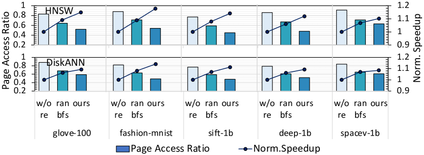
Figure 16: Evaluation of static scheduling of NDSearch. Speedup is normalized to NDSearch without any reordering.

VII-B Results

Performance. Fig. 15 shows the results of throughput (Query Per Second) and the normalized speedup that NDSearch achieves over CPU, GPU, and DeepStore. For DeepStore, we build a channel-level accelerator (DS-c) and chip-level accelerator (DS-cp) as the baselines. The default batch size is set to 2048. Thanks to the high internal parallelism, GPU, DeepStore, and NDSearch can achieve much better performance compared to CPU when processing a large batch of queries. In terms of large datasets, the constructed graph of sift-1b, deep-1b, and spacev-1b could consume more than 500 GBs of memory which exceeds the capacity of VRAM in GPU. Hence, GPU should load a few shards of the data from the SSD several times through the PCIe link. We can observe that DS-c, DS-cp, and NDSearch all outperform the SmartSSD-only design because the SmartSSD-only design does not explore the internal bandwidth and parallelism of the SSD device. Especially, NDSearch achieves up to 7.44$\times$ speedup over the SmartSSD-only design when running DiskANN on sift-1b. It is interesting that DS-cp achieves higher speedup than DS-c on these benchmarks, which differs from the conclusion in  [25]. This is because the workload of graph traversal-based ANNS does not include compute-intensive operations as shown in Fig. 3 like the neural network evaluated in the DeepStore paper. Hence, the limited computing resources will not be the bottleneck of chip-level accelerators. The chip-level accelerators enable DS-cp to process the graph traverse and distance computation locally near the chip and thus DS-cp performs better than DS-c. Compared with DS-cp, NDSearch develops LUN-level accelerators with even higher parallelism. Besides, we utilize and modify the flash chip’s internal multi-LUN and multi-plane operations to support access to vertex vectors and distance computation. The result shows that NDSearch can achieve up to 2.81$\times$ and 2.94$\times$ speedup over DS-cp when running HNSW and DiskANN, respectively. Hence, we can conclude that more fine-grained accelerators at the LUN level are more efficient for ANNS.

It is not difficult to find that NDSearch demonstrates a higher speedup over CPU/GPU when running HNSW/DiskANN on sift-1b/deep-1b are better than those on glove-100/fashion-mnist. This is because the glove-100 and fashion-mnist are much smaller than other datasets. The constructed graphs of these two datasets are able to fit into the main memory of CPU and the memory of the GPU so that CPU/GPU only needs to load the data from the SSD once. Common NDP designs like SmartSSD, DS-c, and DS-cp can hardly outperform CPU/GPU when running ANNS on small datasets because their advantages over CPU/GPU mainly come from reducing SSD I/O read. However, NDSearch further exploits the SSD internal bandwidth with LUN-level accelerators and develops efficient scheduling schemes to increase the searching parallelism. Hence, NDSearch can still achieve up to 5.06$\times$ and 2.12$\times$ speedup over CPU and GPU, respectively.

Statistical significance of improvement. Both the selection of the initial entries on the constructed graphs and the difference amongst the queries affect the performance improvement results. We perform the evaluation by randomly initializing 10 different entry vertices for each of 10 randomly sampled batches of queries. Table I shows the statistical significance of speedup results of NDSearch over CPU in the form of “mean($\pm$standard deviation)”. The mean value of the results are the main results which are illustrated in Fig. 15. From the Table I, we can observe that the standard deviation is at most 11.9% of the mean of the improvement results on different ANNS workloads. Hence, we can conclude that NDSearch achieves stable and robust performance of accelerating ANNS.

TABLE I: Confidential intervals of improvement of NDSearch over CPU

	glove-100	f-mnist	sift-1b
HNSW	$4.28(\pm 0.56)\times$	$5.05(\pm 0.74)\times$	$31.7(\pm 3.78)\times$
DiskANN	$10.96(\pm 1.27)\times$	$12.56(\pm 1.24)\times$	$23.37(\pm 2.28)\times$
	deep-1b	spacev-1b	/
HNSW	$27.49(\pm 2.66)\times$	$28.07(\pm 2.35)\times$	/
DiskANN	$17.86(\pm 1.82)\times$	$21.15(\pm 2.07)\times$	/

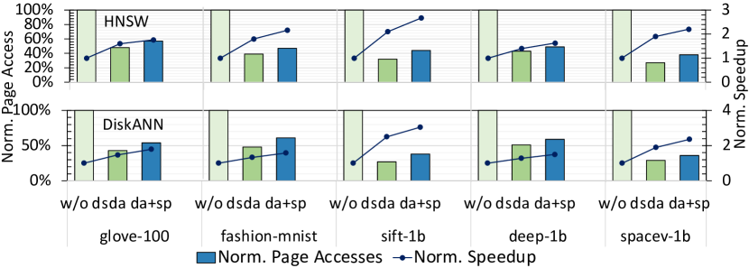
Figure 17: Evaluation of dynamic scheduling. Page access and speedup are normalized to NDSearch without dynamic scheduling.

Scheduling. To evaluate the performance of our reordering method applied to SearSSD, we define a new metric, page access ratio, which equals the ratio of the number of page accesses to the length of the searching trace of a query. A higher page access ratio reflects that each page access returns fewer requested/prefetched vertices, thus indicating poor spatial data locality. We set the page size to 16 KB in this experiment and compute the average page access ratio of a batch (2048) of queries on each benchmark. After applying our reordering method, the bandwidth $\beta$ (defined in Section VI) decreases, which means that the neighbors of each vertex are stored closer to each other. Thus, the neighbors of each vertex are more likely to be stored in the same page, which implicitly reduces the number of page accesses. Fig. 16 shows the comparison of different settings: without reordering (w/o re), with random BFS reordering (ran bfs), and ours. The results indicate that after reordering the vertices and mapping them under the restrictions of multi-plane operation, our method reduces the page access ratio by up to 38% and induces up to 1.17$\times$ speedup over the baseline without reordering.

We also evaluate the contribution of our dynamic scheduling by configuring NDSearch with three different settings: without dynamic scheduling (w/o ds), with dynamic allocating(da) and with dynamic allocating and speculative searching (da+sp). In the setting of NDSearch without dynamic scheduling, each query is just allocated to LUNs sequentially according to the addresses of its targeted vertices that may be flushed and need to be read from the NAND arrays again by another query later. By contrast, with dynamic allocating, different queries that are allocated to the same LUN are potentially able to share the same page access as much as possible. Hence, redundant re-allocating and extra page accesses are avoided. As illustrated in Fig. 17, dynamic allocating can help reduce the page accesses by up to 73% and induce up to 2.67$\times$ speedup. With speculative searching, the page accesses increase because over half of speculated results are not selected, which leads to extra accesses to the second-order neighbors of the queries. However, speculative searching can still further induce up to 1.27$\times$ speedup.

Ablation study.

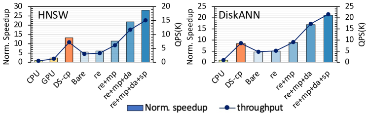
Figure 18: The ablation study of our proposed techniques on NDSearch. The experiments are run on spacev-1b dataset.

We conduct the ablation study of the proposed techniques, including degree ascending BFS reordering (re), multi-plane operation mapping (mp), dynamic allocating (da) and speculative searching (sp) on spacev-1b as shown in Fig. 18. Even without any optimizations, the bare machine of NDSearch (Bare) can still achieve over 4$\times$ speedup over CPU because 1) data transfer via the PCIe is eliminated; and 2) NDSearch does not need frequent access DRAM to fetch the vertices as CPU does to its main memory. Without the dynamic allocating, NDSearch can hardly beat DS-cp though NDSearch achieves larger parallelism and internal bandwidth due to multi-LUN/plane operations. This is because there are redundant operations on the LUN-level accelerators and we actually implement dynamic allocating on DS-cp to maximize its hardware utilization. With all the proposed techniques, NDSearch achieves its optimal performance.

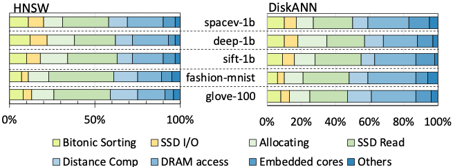
Figure 19: Breakdown of execution time of NDSearch.

Overhead analysis. As illustrated in Fig. 19, NAND read occupies the largest proportion ($24\%-38\%$) of the entire execution time of NDSearch due to the frequent access to feature vectors stored in NAND flash chips. However, compared to the CPU+SSD system, the proportion of SSD I/O read is reduced from $\sim$70% (as shown in Fig. 2) to $\sim$6% thanks to the “filtering” of SearSSD. The latency of the bitonic kernel on FPGA only accounts for at most 12% of the overall latency. We can also observe that running DiskANN requires more DRAM access and execution of embedded cores but fewer SSD reads than HNSW thanks to using the internal DRAM of SSD to cache some hot feature vectors. Generally, DRAM access and execution of embedded cores take 20$\%-35\%$ of the total execution time to maintain the FTL, access LUNCSR, and buffer the temporary results.

ECC and endurance.

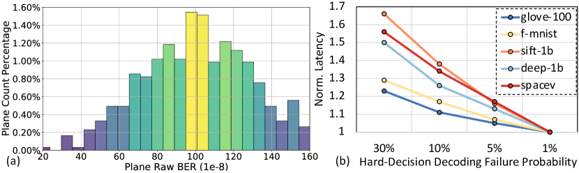
Figure 20: (a) Plane-level distribution of raw bit error rate; (b) Normalized latency of running HNSW workloads with different hard-decision decoding failure probabilities.

We generate the raw bit error rate (BER) statistics of 512 planes in SearSSD following the measured memory BER distribution in  [64] as shown in Fig. 20(a). We set the average BER to $10^{-6}$, which is the typical BER value of current advanced NAND flash. We also consider the fact that the probability of hard-decision LDPC decoding increases since flash memory cell storage reliability gradually degrades. As reported in  [64], even at the mid-late lifetime of flash memory, a hard-decision LDPC decoder can still have a low failure probability ($1\%$, which is also our default case). We evaluate our ECC mechanism in worse scenarios with the hard-decision decoding failure probability set to $30\%$, $10\%$, $5\%$ and $1\%$, respectively. When the hard-decision decoding fails, the soft-decision starts to work on FTL. Following the logistics of fault injection [65], we “inject” the raw BER and the hard-decision decoding failure probability into our simulation environment. As illustrated in Fig. 20(b), In the worst cases where the hard-decision decoding failure probability is 30%, NDSearch is slowed down by between 1.23$\times$ and 1.66$\times$. The slowdown mainly comes from the extra latency of executing soft-decision LDPC ($\sim$ 10 $\mu s$) on FTL and pausing the search iteration. We generally conclude that the plane-level hard-decision LDPC decoder is sufficient in most cases.

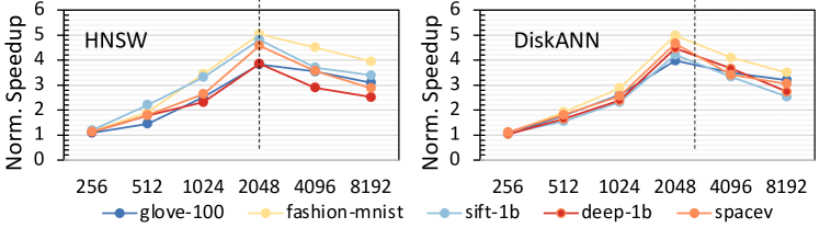
Figure 21: Speedup normalized to DS-cp with different batch sizes.

Batch size. We explore the impact of batch size on performance. As illustrated in Fig. 21, we set the batch size ranging from 256 to 8192 to evaluate NDSearch against DS-cp. We observe that when the batch size is set to 256, NDSearch only has a marginal advantage over DS-cp. The parallelism of relatively fine-grained LUN accelerators cannot be fully exploited when the batch size is small. The irregular access pattern of queries could allocate queries to a few LUN accelerators. In this situation, the advantage of NDSearch is negligible compared to directly processing queries in relatively coarse-grained chip-level accelerators. However, as the batch size increases, NDSearch gains a significant advantage because each LUN has a heavier workload so that the LUN-level parallelism can be fully exploited, and the queries are allocated to most LUNs. The overhead of gathering data from the flash chip to the chip-level accelerators (as aforementioned, only one LUN can be selected when reading data from a flash chip) limited the performance of DS-cp. When the batch size increases to 4196, the speedup of NDSearch begins to decrease because the batch have to be split into two or more sub-batches to process, due to the limited resources setting of our design considering the power budget.

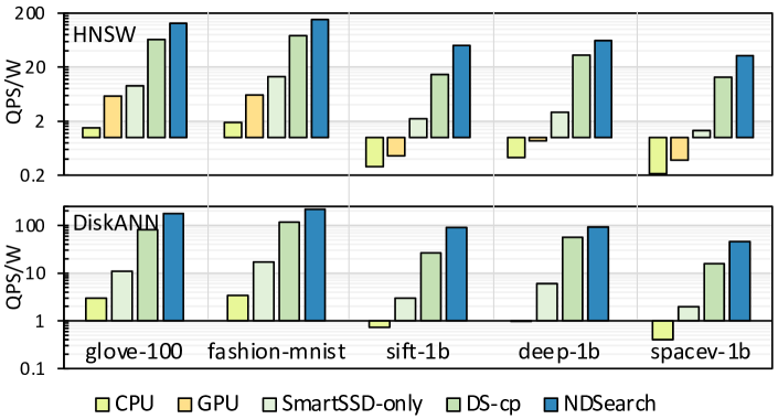
Figure 22: Comparison of energy efficiency over various designs.

TABLE II: Power and Area Breakdown of SearSSD

	Config.	Num.	Power	Area
MAC group	2 MACs	512	1.95 W	15.04 $mm^{2}$
Vgen Buffer	2MB	1	1.71 W	3.18 $mm^{2}$
Alloc Buffer	6MB	1	4.57 W	8.53 $mm^{2}$
Query Queue	24KB	256	5.84 W	9.76 $mm^{2}$
Vaddr Queue	3KB	256	0.87 W	1.47 $mm^{2}$
Output Buffer	1KB	512	0.56W	1.12 $mm^{2}$
ECC Decoder	LDPC	1024	1.18W	2.84 $mm^{2}$
Ctr circuits	-	-	2.14W	1.15 $mm^{2}$
Overall	-	-	18.82W	43.09 $mm^{2}$

Power budget and Energy Efficiency. The power budget of SearSSD is limited by the PCIe interface, which provides $\sim$55W budget  [25] for SearSSD’s design. Table II shows the power breakdown in SearSSD’s design. Overall, the total power of NDSearch is 18.82W, which is within the power budget. Hence, the specialization of NDSearch in the SSD is feasible from the power consumption perspective. Fig.  22 shows the comparison of energy efficiency with various platforms. Basically, the less the data transfer of feature vectors is and the higher internal parallelism the design achieves, the higher energy efficiency is reached. The SmartSSD-only design avoids the data transfer passing through the host CPU. Compared to the SmartSSD-only design, a large amount of data transfer via SSD I/O is avoided in NDSearch, and our NDSearch further reduces the data movement from NAND flash chips by the in-LUN computing. Overall, NDSearch achieves up to 178.68$\times$, 120.87$\times$, 30.06$\times$ and 3.48$\times$ higher energy efficiency than CPU, GPU, the SmartSSD-only design, and DS-cp, respectively.

Area and storage density. Area breakdown of SearSSD is also illustrated in Table II. We estimate the storage density of Samsung 983 DCT [62], which adopts 3-bit V-NAND MLC, as $6Gb/mm^{2}$. After adding the specialized logic inside the SSD, the storage density is reduced to (capacity of SearSSD, 512GB) $\times$ 8b/B / ((capacity of SearSSD, 512GB) $\times$ 8b/B / 6Gb/$mm^{2}$ + 43.9 $mm^{2}$)) = 5.64 Gb/$mm^{2}$, which is acceptable with only 6% density degradation.

VIII Conclusion

In this paper, we present NDSearch, a novel NDP architecture based on SmartSSD, to support the graph-traversal-based ANNS task. We present an in-storage accelerator SearSSD which exploits the LUN-level parallelism inside NAND flash chips to utilize the high internal bandwidth of SSD. We also propose a customized processing model customized for NDP scenarios and implement it on our design to accelerate the graph-traversal-based ANNS. Compared with the previous state-of-the-art NDP designs, NDSearch achieves significant improvements in both throughput and energy efficiency.

References

- [1] “Introduction of vector database,” https://www.pinecone.io/learn/vector-database/.
- [2] “Milvus,” https://milvus.io.
- [3] Y. Park, S. Park, W. Jung, and S.-g. Lee, “Reversed cf: A fast collaborative filtering algorithm using a k-nearest neighbor graph,” Expert Systems with Applications, vol. 42, no. 8, pp. 4022–4028, 2015.
- [4] H. Zhu, M. Long, J. Wang, and Y. Cao, “Deep hashing network for efficient similarity retrieval,” in Proceedings of the AAAI Conference on Artificial Intelligence, vol. 30, no. 1, 2016.
- [5] A. Barman and S. K. Shah, “A graph-based approach for making consensus-based decisions in image search and person re-identification,” IEEE transactions on pattern analysis and machine intelligence, 2019.
- [6] J. Ma, Z. Zhao, X. Yi, J. Yang, M. Chen, J. Tang, L. Hong, and E. H. Chi, “Off-policy learning in two-stage recommender systems,” in Proceedings of The Web Conference 2020, 2020, pp. 463–473.
- [7] Z. Zheng, X. Yang, Z. Yu, L. Zheng, Y. Yang, and J. Kautz, “Joint discriminative and generative learning for person re-identification,” in proceedings of the IEEE/CVF conference on computer vision and pattern recognition, 2019, pp. 2138–2147.
- [8] M. Naumov, D. Mudigere, H.-J. M. Shi, J. Huang, N. Sundaraman, J. Park, X. Wang, U. Gupta, C.-J. Wu, A. G. Azzolini et al., “Deep learning recommendation model for personalization and recommendation systems,” arXiv preprint arXiv:1906.00091, 2019.
- [9] H. Guo, R. Tang, Y. Ye, Z. Li, and X. He, “Deepfm: a factorization-machine based neural network for ctr prediction,” arXiv preprint arXiv:1703.04247, 2017.
- [10] L. Amsaleg and H. Jégou, “Datasets for approximate nearest neighbor search,” http://corpus-texmex.irisa.fr/.
- [11] A. Babenko and V. Lempitsky, “Efficient indexing of billion-scale datasets of deep descriptors,” in Proceedings of the IEEE Conference on Computer Vision and Pattern Recognition, 2016, pp. 2055–2063.
- [12] “Spacev1b: A billion-scale vector dataset for text descriptors,” https://github.com/microsoft/SPTAG/tree/main/datasets/SPACEV1B.
- [13] S. Arya, D. M. Mount, N. S. Netanyahu, R. Silverman, and A. Y. Wu, “An optimal algorithm for approximate nearest neighbor searching fixed dimensions,” Journal of the ACM (JACM), vol. 45, no. 6, pp. 891–923, 1998.
- [14] A. Andoni and P. Indyk, “Near-optimal hashing algorithms for approximate nearest neighbor in high dimensions,” in 2006 47th annual IEEE symposium on foundations of computer science (FOCS’06). IEEE, 2006, pp. 459–468.
- [15] C. Fu, C. Xiang, C. Wang, and D. Cai, “Fast approximate nearest neighbor search with the navigating spreading-out graph,” Proceedings of the VLDB Endowment, vol. 12, no. 5, pp. 461–474, 2019.
- [16] Y. A. Malkov and D. A. Yashunin, “Efficient and robust approximate nearest neighbor search using hierarchical navigable small world graphs,” IEEE transactions on pattern analysis and machine intelligence, vol. 42, no. 4, pp. 824–836, 2018.
- [17] S. J. Subramanya, F. Devvrit, H. Simhadri, R. Krishnawamy, and R. Kadekodi, “Diskann: Fast accurate billion-point nearest neighbor search on a single node,” Advances in Neural Information Processing Systems, vol. 32, pp. 13 771–13 781, 2019.
- [18] Y. Matsui, T. Yamaguchi, and Z. Wang, “Cvpr2020 tutorial on image retrieval in the wild,” https://matsui528.github.io/cvpr2020_tutorial_retrieval/, 2020.
- [19] R. Chen, S. Siriyal, and V. Prasanna, “Energy and memory efficient mapping of bitonic sorting on fpga,” in Proceedings of the 2015 ACM/SIGDA International Symposium on Field-Programmable Gate Arrays, 2015, pp. 240–249.
- [20] “ANN datasets,” https://big-ann-benchmarks.com.
- [21] Y. Malkov, A. Ponomarenko, A. Logvinov, and V. Krylov, “Approximate nearest neighbor algorithm based on navigable small world graphs,” Information Systems, vol. 45, pp. 61–68, 2014.
- [22] “Diskann,” https://github.com/microsoft/DiskANN.
- [23] “Hnswlib - fast approximate nearest neighbor search,” https://github.com/nmslib/hnswlib.
- [24] “Gpuacc,” https://github.com/harsha-simhadri/big-ann-benchmarks/blob/main/t3/LEADERBOARDS_PUBLIC.md.
- [25] V. S. Mailthody, Z. Qureshi, W. Liang, Z. Feng, S. G. De Gonzalo, Y. Li, H. Franke, J. Xiong, J. Huang, and W.-m. Hwu, “Deepstore: In-storage acceleration for intelligent queries,” in Proceedings of the 52nd Annual IEEE/ACM International Symposium on Microarchitecture, 2019, pp. 224–238.
- [26] N. Sundaram, N. Satish, M. M. A. Patwary, S. R. Dulloor, M. J. Anderson, S. G. Vadlamudi, D. Das, and P. Dubey, “Graphmat: high performance graph analytics made productive,” Proceedings of the VLDB Endowment, vol. 8, no. 11, pp. 1214–1225, 2015.
- [27] M. Yan, X. Hu, S. Li, A. Basak, H. Li, X. Ma, I. Akgun, Y. Feng, P. Gu, L. Deng et al., “Alleviating irregularity in graph analytics acceleration: a hardware/software co-design approach,” in Proceedings of the 52nd Annual IEEE/ACM International Symposium on Microarchitecture, 2019, pp. 615–628.
- [28] J. H. Lee, H. Zhang, V. Lagrange, P. Krishnamoorthy, X. Zhao, and Y. S. Ki, “Smartssd: Fpga accelerated near-storage data analytics on ssd,” IEEE Computer architecture letters, vol. 19, no. 2, pp. 110–113, 2020.
- [29] S. Salamat, A. Haj Aboutalebi, B. Khaleghi, J. H. Lee, Y. S. Ki, and T. Rosing, “Nascent: Near-storage acceleration of database sort on smartssd,” in The 2021 ACM/SIGDA International Symposium on Field-Programmable Gate Arrays, 2021, pp. 262–272.
- [30] J.-H. Kim, Y.-R. Park, J. Do, S.-Y. Ji, and J.-Y. Kim, “Accelerating large-scale graph-based nearest neighbor search on a computational storage platform,” IEEE Transactions on Computers, pp. 1–1, 2022.
- [31] K. Fukunaga and P. M. Narendra, “A branch and bound algorithm for computing k-nearest neighbors,” IEEE transactions on computers, vol. 100, no. 7, pp. 750–753, 1975.
- [32] K. Eshghi and R. Micheloni, “Ssd architecture and pci express interface,” in Inside solid state drives (SSDs). Springer, 2013, pp. 19–45.
- [33] “Lunorganization,” https://arxiv.org/pdf/1711.11427.pdf.
- [34] “Lunorganization2,” http://www.onfi.org/-/media/client/onfi/specs/onfi_4_1_gold.pdf?la=en.
- [35] H. Semiconductor et al., “Open nand flash interface specification,” Technical Report ONFI, 2006.
- [36] “Openssd Peer-to-Peer (P2P) - Xilinx XRT.” [Online]. Available: https://media-www.micron.com/-/media/client/onfi/specs/
- [37] T.-S. Chung, D.-J. Park, S. Park, D.-H. Lee, S.-W. Lee, and H.-J. Song, “A survey of flash translation layer,” Journal of Systems Architecture, vol. 55, no. 5-6, pp. 332–343, 2009.
- [38] M. Wilkening, U. Gupta, S. Hsia, C. Trippel, C.-J. Wu, D. Brooks, and G.-Y. Wei, “Recssd: near data processing for solid state drive based recommendation inference,” in Proceedings of the 26th ACM International Conference on Architectural Support for Programming Languages and Operating Systems, 2021, pp. 717–729.
- [39] K. K. Matam, G. Koo, H. Zha, H.-W. Tseng, and M. Annavaram, “Graphssd: Graph semantics aware ssd,” in Proceedings of the 46th International Symposium on Computer Architecture, ser. ISCA ’19. New York, NY, USA: Association for Computing Machinery, 2019, p. 116–128. [Online]. Available: https://doi.org/10.1145/3307650.3322275
- [40] C. Li, Y. Wang, C. Liu, S. Liang, H. Li, and X. Li, “GLIST: Towards In-Storage graph learning,” in 2021 USENIX Annual Technical Conference (USENIX ATC 21). USENIX Association, Jul. 2021, pp. 225–238. [Online]. Available: https://www.usenix.org/conference/atc21/presentation/li-cangyuan
- [41] S.-W. Jun, A. Wright, S. Zhang, S. Xu, and Arvind, “Grafboost: Using accelerated flash storage for external graph analytics,” in Proceedings of the 45th Annual International Symposium on Computer Architecture, ser. ISCA ’18. IEEE Press, 2018, p. 411–424. [Online]. Available: https://doi.org/10.1109/ISCA.2018.00042
- [42] S. Liang, Y. Wang, Y. Lu, Z. Yang, H. Li, and X. Li, “Cognitive SSD: A deep learning engine for In-Storage data retrieval,” in 2019 USENIX Annual Technical Conference (USENIX ATC 19). Renton, WA: USENIX Association, Jul. 2019, pp. 395–410. [Online]. Available: https://www.usenix.org/conference/atc19/presentation/liang
- [43] J. Lin, L. Liang, Z. Qu, I. Ahmad, L. Liu, F. Tu, T. Gupta, Y. Ding, and Y. Xie, “Inspire: In-storage private information retrieval via protocol and architecture co-design,” in Proceedings of the 49th Annual International Symposium on Computer Architecture, ser. ISCA ’22. New York, NY, USA: Association for Computing Machinery, 2022, p. 102–115. [Online]. Available: https://doi.org/10.1145/3470496.3527433
- [44] C. Gao, X. Xin, Y. Lu, Y. Zhang, J. Yang, and J. Shu, “Parabit: Processing parallel bitwise operations in nand flash memory based ssds,” in MICRO-54: 54th Annual IEEE/ACM International Symposium on Microarchitecture, 2021, pp. 59–70.
- [45] W. Niu, J. Guan, X. Shen, Y. Wang, G. Agrawal, and B. Ren, “Gcd2: A globally optimizing compiler for mapping dnns to mobile dsps,” in 2022 55th IEEE/ACM International Symposium on Microarchitecture (MICRO), 2022, pp. 512–529.
- [46] H.-W. Hu, W.-C. Wang, Y.-H. Chang, Y.-C. Lee, B.-R. Lin, H.-M. Wang, Y.-P. Lin, Y.-M. Huang, C.-Y. Lee, T.-H. Su, C.-C. Hsieh, C.-M. Hu, Y.-T. Lai, C.-K. Chen, H.-S. Chen, H.-P. Li, T.-W. Kuo, M.-F. Chang, K.-C. Wang, C.-H. Hung, and C.-Y. Lu, “Ice: An intelligent cognition engine with 3d nand-based in-memory computing for vector similarity search acceleration,” in 2022 55th IEEE/ACM International Symposium on Microarchitecture (MICRO), 2022, pp. 763–783.
- [47] R. P. Stanley, “Enumerative combinatorics, volume 1. wadsworth,” Inc. California, 1986.
- [48] A. George, M. T. Heath, J. Liu, and E. Ng, “Solution of sparse positive definite systems on a shared-memory multiprocessor,” International journal of parallel programming, vol. 15, no. 4, pp. 309–325, 1986.
- [49] K. Zhao, W. Zhao, H. Sun, X. Zhang, N. Zheng, and T. Zhang, “LDPC-in-SSD: Making advanced error correction codes work effectively in solid state drives,” in 11th USENIX Conference on File and Storage Technologies (FAST 13), 2013, pp. 243–256.
- [50] R. Jose and A. Pe, “Analysis of hard decision and soft decision decoding algorithms of ldpc codes in awgn,” in 2015 IEEE International Advance Computing Conference (IACC). IEEE, 2015, pp. 430–435.
- [51] T. Tian, C. R. Jones, J. D. Villasenor, and R. D. Wesel, “Selective avoidance of cycles in irregular ldpc code construction,” IEEE Transactions on Communications, vol. 52, no. 8, pp. 1242–1247, 2004.
- [52] R. Koetter and A. Vardy, “Algebraic soft-decision decoding of reed-solomon codes,” IEEE Transactions on Information Theory, vol. 49, no. 11, pp. 2809–2825, 2003.
- [53] B. Coleman, S. Segarra, A. Shrivastava, and A. Smola, “Graph reordering for cache-efficient near neighbor search,” arXiv preprint arXiv:2104.03221, 2021.
- [54] L. Auroux, M. Burelle, and R. Erra, “Reordering very large graphs for fun & profit,” in International Symposium on Web AlGorithms, 2015.
- [55] H. R. Lewis, “Michael r. garey and david s. johnson. computers and intractability. a guide to the theory of np-completeness. wh freeman and company, san francisco1979, x+ 338 pp.” The Journal of Symbolic Logic, vol. 48, no. 2, pp. 498–500, 1983.
- [56] A. Caprara and J.-J. Salazar-González, “Laying out sparse graphs with provably minimum bandwidth,” INFORMS Journal on Computing, vol. 17, no. 3, pp. 356–373, 2005.
- [57] “Cuhnsw,” https://github.com/js1010/cuhnsw.
- [58] J. Pennington, R. Socher, and C. D. Manning, “Glove: Global vectors for word representation,” in Proceedings of the 2014 conference on empirical methods in natural language processing (EMNLP), 2014, pp. 1532–1543.
- [59] H. Xiao, K. Rasul, and R. Vollgraf, “Fashion-mnist: a novel image dataset for benchmarking machine learning algorithms,” arXiv preprint arXiv:1708.07747, 2017.
- [60] N. Agrawal, V. Prabhakaran, T. Wobber, J. D. Davis, M. Manasse, and R. Panigrahy, “Design tradeoffs for ssd performance,” in USENIX 2008 Annual Technical Conference, ser. ATC’08. USA: USENIX Association, 2008, p. 57–70.
- [61] “huaicheng/ssdsim,” https://github.com/huaicheng/ssdsim.
- [62] “Download - simplessd 2.0,” https://docs.simplessd.org/en/v2.0.12/download.html#nvme-ssd.
- [63] “Cacti 6.5,” http://www.hpl.hp.com/research/cacti.
- [64] K. Zhao, W. Zhao, H. Sun, X. Zhang, N. Zheng, and T. Zhang, “LDPC-in-SSD: Making advanced error correction codes work effectively in solid state drives,” in 11th USENIX Conference on File and Storage Technologies (FAST 13), 2013, pp. 243–256.
- [65] B. Fang, D. Wang, S. Jin, Q. Koziol, Z. Zhang, Q. Guan, S. Byna, S. Krishnamoorthy, and D. Tao, “Characterizing impacts of storage faults on hpc applications: A methodology and insights,” in 2021 IEEE International Conference on Cluster Computing (CLUSTER). IEEE, 2021, pp. 409–420.