Scale-invariant magnetic anisotropy in $\alpha$-RuCl₃: A quantum Monte Carlo study

Abstract

We compute the rotational anisotropy of the free energy of $\alpha$-RuCl₃ in an external magnetic field. This quantity, known as the magnetotropic susceptibility, $k$, relates to the second derivative of the free energy with respect to the angle of rotation. We have used approximation-free, auxiliary-field quantum Monte Carlo simulations for a realistic model of $\alpha$-RuCl₃ and optimized the path integral to alleviate the negative sign problem. This allows us to reach temperatures down to $30~{}\rm{K}$ — an energy scale below the dominant Kitaev coupling. We demonstrate that the magnetotropic susceptibility in this model of $\alpha$-RuCl₃ displays unique scaling, $k=Tf(B/T)$, with distinct scaling functions $f$ at high and low temperatures. In comparison, for the XXZ Heisenberg model, the scaling $k=Tf(B/T)$ breaks down at a temperature scale where the uniform spin susceptibility deviates from the Curie law (i.e. at the energy scale of the exchange interactions) and never recovers at low temperatures. Our findings suggest that correlations in $\alpha$-RuCl₃ lead to degrees of freedom that respond isotropically to a magnetic field. One possible interpretation for the apparent scale-invariance observed in experiments could be fractionalization of the spin degrees of freedom in the extended Kitaev model.

Introduction.— Quantum spin liquids are believed to harbor exotic fractionalized excitations that defy the conventional categories of fermions and bosons. The Kitaev model, originally proposed by Alexei Kitaev in 2006 [1], has served as a paradigm in this context, offering an exact solution for a quantum spin liquid state on the honeycomb lattice.

$\alpha$-RuCl₃ has emerged as a leading candidate for realizing the Kitaev spin liquid  [2, 3, 4]. Numerous experiments have probed its thermodynamic and dynamical properties and have reached the conclusion that there is a dominant Kitaev exchange interaction [5, 6, 7, 8, 9, 10, 11, 12, 13, 14, 15]. One intriguing observation is the emergence of scale-invariance at low temperatures and in high magnetic fields [16]. The aim of this Letter is to bridge this experimental observation in $\alpha$-RuCl₃ with approximation-free quantum Monte Carlo (QMC) simulations.

QMC methods allow for the numerical solution of target models for a given lattice size and temperature without further approximations. Frustrated spin systems, like Kitaev materials, generically suffer from the infamous negative sign problem that leads to an exponential increase in the required computational power as a function of the volume $V$ of the system and inverse temperature $\beta$ [17]. Since the severity of this problem depends on the specific formulations, optimization strategies to alleviate it can be put forward. Indeed, in our recent publication [18], we have developed a fermion QMC approach using the auxiliary-field QMC (AFQMC) algorithm for fermions [19, 20, 21] to tackle frustrated spin models. The generalized Kitaev model, describing materials such as layered iridates and $\alpha$-RuCl₃, benefits from this approach. It mitigates the severity of the negative sign problem and enables QMC simulations at temperatures well below the magnetic exchange scale. This opens up a window of temperatures relevant to experiments. We demonstrate that this method reproduces the experimental magnetotropic susceptibility in $\alpha$-RuCl₃ [16].

Minimal models for Kitaev materials.— We consider first-neighbor, Kitaev $K_{1}$, and off-diagonal symmetric, $\Gamma_{1}$, couplings, as well as first-neighbor (third-neighbor) Heisenberg couplings, $J_{1}$ ($J_{3}$), on the honeycomb lattice:

$$\hat{H}_{s} = \sum_{\boldsymbol{i}\in A,\gamma}\left[K_{1}\hat{S}_{\boldsymbol{i}}^{\gamma}\hat{S}_{\boldsymbol{i}+\boldsymbol{\delta}_{\gamma}}^{\gamma}+\Gamma_{1}\left(\hat{S}_{\boldsymbol{i}}^{\alpha}\hat{S}_{\boldsymbol{i}+\boldsymbol{\delta}_{\gamma}}^{\beta}+\hat{S}_{\boldsymbol{i}}^{\beta}\hat{S}_{\boldsymbol{i}+\boldsymbol{\delta}_{\gamma}}^{\alpha}\right)\right]$$ (1)

$$+\sum_{\boldsymbol{i}\in A,\boldsymbol{\delta}_{\gamma}}J_{1}\hat{\boldsymbol{S}}_{\boldsymbol{i}}\cdot\hat{\boldsymbol{S}}_{\boldsymbol{i}+\boldsymbol{\delta}_{\gamma}}+\sum_{\boldsymbol{i}\in A,\boldsymbol{\delta}^{\prime}_{\gamma}}J_{3}\hat{\boldsymbol{S}}_{\boldsymbol{i}}\cdot\hat{\boldsymbol{S}}_{\boldsymbol{i}+\boldsymbol{\delta}^{\prime}_{\gamma}}.$$

Here $\boldsymbol{i}$ runs over the $A$ sublattice and $\boldsymbol{i}+\boldsymbol{\delta}_{\gamma}$ ($\boldsymbol{i}+\boldsymbol{\delta}^{\prime}_{\gamma}$) over the first (third) neighbors. For the first term $(\gamma,\alpha,\beta)=(1,2,3)$ for the $X$ bonds, $(\gamma,\alpha,\beta)=(2,3,1)$ for the $Y$ bonds, and $(\gamma,\alpha,\beta)=(3,1,2)$ for the $Z$ bonds on each lattice site [see Fig. 1 (a)].

To study the magnetotropic susceptibility of $\alpha$-RuCl₃ under high magnetic fields reported in Ref. [16], we add a Zeeman term to produce the total Hamiltonian

$$\hat{H}=\hat{H}_{s}-\mu_{B}\sum_{\boldsymbol{i}}\boldsymbol{B}\cdot\hat{g}\cdot\hat{\boldsymbol{S}}_{\boldsymbol{i}},$$ (2)

where the direction of the magnetic field in the cubic spin basis corresponds to $\boldsymbol{B}||[xyz]$ (see Fig. 1 (a)). In Kitaev materials such as $\alpha$-RuCl₃, the $[111]$ axis aligns with the $\boldsymbol{c}$ axis, perpendicular to the honeycomb lattice, whereas the $[11\bar{2}]$ and $[\bar{1}10]$ axes correspond to the in-plane $\boldsymbol{a}$ and $\boldsymbol{b}$ axes, respectively (see Fig. 1(a)). We adopt the parametrization $\boldsymbol{B}=B\left[\sin(\varphi)\sin(\theta)\boldsymbol{e}_{a}+\cos(\varphi)\sin(\theta)\boldsymbol{e}_{b}+\cos(\theta)\boldsymbol{e}_{c}\right]$, where the unit vectors $\boldsymbol{e}_{a}$, $\boldsymbol{e}_{b}$, and $\boldsymbol{e}_{c}$ point along the $[11\bar{2}]$, $[\bar{1}10]$, and $[111]$ directions, respectively. $\hat{g}=g^{\alpha,\alpha^{\prime}}$ represents the anisotropic $g$ factor, which contains only diagonal entries in the aforementioned directions, specifically $(g_{a},g_{b},g_{c})=(2.3,2.3,1.3)$ [22, 23].

Hamiltonian (1) was simulated using the AFQMC method of Ref. [18]. Here we adopt an Abrikosov fermion representation of the spin-1/2 degree of freedom: $\hat{\boldsymbol{S}}=\frac{1}{2}\hat{\boldsymbol{f}}^{\dagger}\hat{\boldsymbol{\sigma}}\hat{\boldsymbol{f}}^{\phantom{\dagger}}$ with $\hat{\boldsymbol{f}}^{\dagger}\equiv(\hat{f}^{\dagger}_{\uparrow},\hat{f}^{\dagger}_{\downarrow})$, $\boldsymbol{\sigma}$ the vector of Pauli matrices, and with the constraint $\hat{\boldsymbol{f}}^{\dagger}\hat{\boldsymbol{f}}^{\phantom{\dagger}}=1$. The key point is to consider a space of path integral formulations and to maximize the average sign over this space. As we will see, this optimization process allows us to reach temperatures down to $30~{}\rm{K}$ . We use a Trotter discretization in the range $\Delta\tau\in[0.01,0.05]$ depending upon the temperature. For this range of $\Delta\tau$, the systematic error is contained within our error bars. We simulated lattices with $L\times L$ unit cells (each containing two spins, i.e., $V=2L^{2}$ lattice sites on the honeycomb lattice) and periodic boundary conditions.

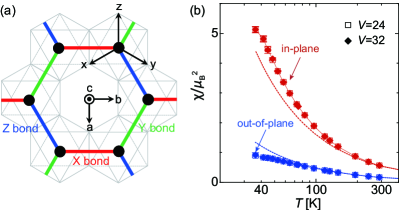
Figure 1: (a) Schematic of our model for $\alpha$-RuCl₃. Spin-1/2 degrees of freedom, $\hat{\boldsymbol{S}}_{\boldsymbol{i}}$, are situated on the honeycomb lattice and are subject to first-neighbor Kitaev $K_{1}$, and off-diagonal symmetric $\Gamma_{1}$, exchange interactions, as well as first-neighbor ($J_{1}$) and third-neighbor ($J_{3}$) Heisenberg couplings. The RuCl₆ octahedra within the honeycomb lattice, along with the definition of the cubic spin-space axes $[x,y,z]$ as indicated in the octahedron’s top view, are illustrated. (b) $T$ dependence of the in-plane and out-of-plane uniform spin susceptibilities $\chi$. The dashed line is a fit to Curie’s law at high temperatures.

Uniform spin susceptibilities.— A key question is whether our QMC approach allows one to reach temperature scales that are relevant to experiments for Kitaev materials. To determine the lowest accessible temperature, we measure the spin susceptibility tensor $\hat{\chi}=\chi^{\alpha,\alpha^{\prime}}$,

$$\chi^{\alpha,\alpha^{\prime}}(\boldsymbol{q})=\int_{0}^{\beta}\text{d}\tau\Big{[}\langle\hat{\boldsymbol{O}}^{\alpha}_{\boldsymbol{q}}(\tau)\hat{\boldsymbol{O}}^{\alpha^{\prime}}_{-\boldsymbol{q}}(0)\rangle-\langle\hat{\boldsymbol{O}}^{\alpha}_{\boldsymbol{q}}\rangle\langle\hat{\boldsymbol{O}}^{\alpha^{\prime}}_{-\boldsymbol{q}}\rangle\Big{]}$$ (3)

where $\hat{\boldsymbol{O}}^{\alpha}_{\boldsymbol{q}}=\frac{\mu_{B}g^{\alpha,\alpha}}{\sqrt{V}}\sum_{\boldsymbol{r}}e^{i\boldsymbol{q}\cdot\boldsymbol{r}}\left(\hat{S}_{\boldsymbol{r},A}^{\alpha}+\hat{S}_{\boldsymbol{r},B}^{\alpha}e^{i\boldsymbol{q}\boldsymbol{R}}\right)$. Here $\boldsymbol{r}$ runs over the $A$ sublattice (or unit cell) and $\boldsymbol{R}=2/3(\boldsymbol{A}_{2}-\boldsymbol{A}_{1}/2)$ with the primitive lattice vectors $\boldsymbol{A}_{1}=(1,0)$ and $\boldsymbol{A}_{2}=(\frac{1}{2},\frac{\sqrt{3}}{2})$. Projecting $\chi^{\alpha,\alpha^{\prime}}(\boldsymbol{q=\Gamma})$ onto the in-plane (out-of-plane) direction yields the in-plane (out-of-plane) uniform spin susceptibility $\chi_{\parallel}=\boldsymbol{e}_{ab}^{\text{T}}\hat{\chi}\boldsymbol{e}_{ab}$ ($\chi_{\perp}=\boldsymbol{e}_{c}^{\text{T}}\hat{\chi}\boldsymbol{e}_{c}$).

Figure 1 (b) plots the results down to the lowest accessible temperature. For model parameters proposed to describe $\alpha$-RuCl₃ [24], $(J_{1},J_{3},K_{1},\Gamma_{1})=(-5.8,5.8,-58,29)~{}{\rm K}$, we can reach temperatures down to $T\sim 30~{}\rm{K}$ on the relatively large lattice size $V=32$, which is beyond the accessible lattice sizes in exact diagonalization calculations at finite temperature (i.e., $V=24$ sites [25]). On the experimental front, $\alpha$-RuCl₃ exhibits zigzag spin order at low temperatures, but proximity to the Kitaev spin liquid suggests that high energy features of this material are described by Majorana fermions [8, 9]. These fermions will hence only show up in finite-temperature properties in an intermediate temperature range bounded by the ordering temperature from below and the coherence scale of the Majorana fermions from above. Experimentally, this temperature range corresponds to $T\in[10,100]~{}\rm{K}$ [8, 9], and it is remarkable to observe that the QMC simulations can access this regime before the negative sign problem becomes too severe. Our numerical results, as a function of decreasing temperature, not only confirm the deviation from a Curie law at high temperatures but also demonstrate a clear trend in $\chi_{\parallel}>\chi_{\perp}$, which exhibits similar behavior as experiments in $\alpha$-RuCl₃ reported in Refs. [5, 6, 7, 13].

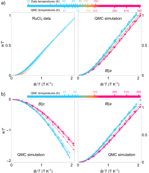
Figure 2: (a) The magnetotropic susceptibility per Ru atom of $\alpha$-RuCl₃ normalized by temperature $k/T$ versus magnetic field normalized by temperature $B/T$. Both $k$ and $T$ are given in energy units for the vertical axis, making $k/T$ a dimensionless quantity. $T$ is in kelvin for the lower axis. Left panel a shows the experimental data from [16] and right panel shows our QMC calculations using the model parameters described in the text. The applied magnetic field is oriented close to the $\boldsymbol{a}$-$\boldsymbol{b}$ plane. The collapse of blue curves in both the experimental data and the calculated magnetotropic susceptibility represent scaling behavior in the temperature range $T\in[20,70]~{}\rm{K}$. Above this temperature, the experimental data deviates toward the paramagnetic scaling (red curves) observed at high temperatures in the QMC calculations. Limited field range at these temperatures prevents experimental access to the high-temperature scaling regime. (b) Same as (a) for varying magnetic field directions in the QMC calculations.

Magnetotropic susceptibility.— We now focus our attention on recent measurements for $\alpha$-RuCl₃ concerning the so-called magnetotropic susceptibility over a wide range of temperatures and magnetic fields [16]. This quantity is defined as the second derivative of the free energy with respect to the rotation angle of the magnetic field and is the thermodynamic coefficient associated with the magnetic anisotropy. In our QMC simulations, and as detailed in the Supplemental Material, the magnetotropic susceptibility in the rotation plane perpendicular to the unit vector $\boldsymbol{e}$ is computed using [26]

$$k = \frac{1}{V}\Big{[}\mu_{B}\boldsymbol{e}\times\left(\boldsymbol{e}\times\boldsymbol{B}\right)\cdot\hat{g}\cdot\langle\hat{\boldsymbol{S}}_{tot}\rangle$$ (4)

$$- \mu_{B}^{2}\int_{0}^{\beta}d\tau\,\ \Big{[}\langle\left(\boldsymbol{e}\times\boldsymbol{B}\right)\cdot\hat{g}\cdot\hat{\boldsymbol{S}}_{tot}(\tau)\left(\boldsymbol{e}\times\boldsymbol{B}\right)\cdot\hat{g}\cdot\hat{\boldsymbol{S}}_{tot}(0)\rangle$$

$$~{}~{}~{}~{}-\langle\left(\boldsymbol{e}\times\boldsymbol{B}\right)\cdot\hat{g}\cdot\hat{\boldsymbol{S}}_{tot}\rangle^{2}\Big{)}\Big{]}$$

with $\hat{\boldsymbol{S}}_{tot}=\sum_{\boldsymbol{i},\alpha}\hat{S}_{\boldsymbol{i}}^{\alpha}$ and an imaginary time $\tau$. Figure 2 presents the results for the magnetotropic susceptibility $k$, with respect to temperature and magnetic field in the $\boldsymbol{a}$-$\boldsymbol{b}$ plane, and compares them to experiments for $\alpha$-RuCl₃ [16]. The magnetotropic susceptibility measurements have shown temperature and magnetic field scaling behavior of the form $k=Tf(B/T)$ over the temperature range bounded by the spin ordering temperature and the coherence scale of Majorana fermions, $T\approx[10,100]~{}\rm{K}$ (see the left panel of Fig. 2 (a)). Our QMC data shown in the right panel of Fig. 2 (a) quantitatively reproduces this scaling behavior below the magnetic exchange scale. Furthermore, our numerical results reveal that as the temperature increases, there is a departure from the low-temperature scaling, and we then observe a distinct scaling behavior at high temperatures. The experimental data shows the departure from the low-temperature scaling, but higher magnetic fields are required to reach the high-temperature, paramagnetic scaling. Moreover, for the other magnetic field directions in the QMC data, for instance, along the $\boldsymbol{c}$ direction (the left panel of Fig. 2 (b)) and the $\boldsymbol{b}$ direction (the right panel of Fig. 2 (b)), the scaling behavior remains observable and consistent at both high and low temperatures.

Scaling behavior of the form $k=Tf(B/T)$ is satisfied for independent local moments for any anisotropic $g$-factor (see Supplemental Material). This is expected for any spin system when the temperature exceeds the magnetic exchange energy and the scaling is expected to break down below this energy scale. However, the case of $\alpha$-RuCl₃ reveals a more complex scenario. Our QMC data show two distinct scaling behaviors: scaling that is characteristic of a free spin at high temperatures, as well as a new emergent scaling at low temperatures.

To underline the uniqueness of the low-temperature scaling behavior observed in $\alpha$-RuCl₃, we now compare our previous findings with those from a non-frustrated spin model, where no fractionalization occurs. We consider the XXZ model on the honeycomb lattice, $\hat{H}_{s}=\sum_{\langle\boldsymbol{i},\boldsymbol{j}\rangle}J\left[\hat{S}^{x}_{\boldsymbol{i}}\cdot\hat{S}^{x}_{\boldsymbol{j}}+\hat{S}^{y}_{\boldsymbol{i}}\cdot\hat{S}^{y}_{\boldsymbol{j}}\right]+\left[J+J_{z}\right]\hat{S}_{\boldsymbol{i}}^{z}\hat{S}_{\boldsymbol{j}}^{z}$, and present QMC results for $J_{z}/J=-0.5$ in Fig. 3.

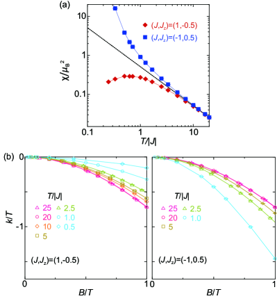
Figure 3: (a) $T$ dependence of the uniform spin susceptibilities $\chi$ in the non-frustrated spin model on the honeycomb lattice with $V=72$ (see the main text). The dashed line represents a fit to Curie’s law at high temperatures. (b) The magnetotropic susceptibility normalized by temperature $k/T$ versus magnetic field normalized by temperature $B/T$. The magnetic field is considered in the out-of-plane direction of the honeycomb lattice.

As the temperature decreases, the uniform spin susceptibility $\chi$ deviates from the high-temperature Curie law (see Fig. 3 (a)). In the ferromagnetic case, $J=-1$, $\chi$ grows and ultimately diverges at low temperatures, whereas in the antiferromagnetic case, $J=1$, local antiferromagnetic correlations lead to a suppression of $\chi$ with respect to the high-temperature Curie law. At low temperatures $\chi$ will scale to a constant value, reflecting the presence of Goldstone modes. As is apparent from the data in Fig. 3 (b), our numerical results for the magnetotropic susceptibility confirm the high-temperature scaling behavior: all curves for $T/|J|\geq 5$ collapse when scaled in this way. The breakdown of the data collapse $k=Tf(B/T)$ agrees with the temperature scale where the deviation from the Curie law behavior is observed in the susceptibility. Unlike in Fig. 2 for the extended Kitaev model, where the low temperature data collapses into a new scaling form, the XXZ model exhibits no such re-collapse at low temperatures.

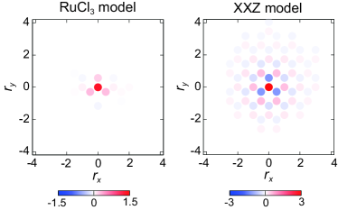
Figure 4: Real-space torque correlations $\langle t_{\boldsymbol{r}}t_{\boldsymbol{0}}\rangle$ for the RuCl₃ model ($T=41.4~{}\rm{K}$ and $B=5~{}\rm{T}$) and the XXZ model with $(J,J_{z})=(1,-0.5)$ ($T/|J|=0.5$ and $\mu_{B}B/|J|=0.1$). Here, the magnetic field is considered in the out-of-plane direction.

Summary and interpretation.— We have investigated the behavior of the magnetotropic susceptibility, $k$, in a realistic magnetic model of $\alpha$-RuCl₃ in an external magnetic field. Employing approximation-free, auxiliary-field quantum Monte Carlo simulations, we have explored the rotational anisotropy of the free energy, highlighting the intricate relationship between temperature $T$, magnetic field $B$, and the unique scaling behavior of $k$. Our results show high- and low-temperature scaling behavior, $k=Tf(B/T)$, with distinct high- and low-temperature scaling functions, $f$. The low-temperature scaling is in quantitative agreement with the experimental data [16] (Fig. 2). The high-temperature scaling, which is inaccessible to experiments, is generic to all spin systems: when the thermal energy exceeds the magnetic exchange, spin systems behave as independent local moments. The low-temperature scaling, on the other hand, is unique to our model of $\alpha$-RuCl₃ and is not present for the un-frustrated XXZ model.

The magnetotropic susceptibility relates to the fluctuations of the torque $\frac{\partial F}{\partial\theta}=\mu_{B}\sum_{\boldsymbol{i}}\hat{t}_{\boldsymbol{i}}$ with $\hat{t}_{\boldsymbol{i}}=(\boldsymbol{e}\times\boldsymbol{B})\cdot\hat{g}\cdot\hat{\boldsymbol{S}}_{\boldsymbol{i}}$. A naive explanation for the emergence of scaling at low temperature would be proximity to a critical point at which long wave length fluctuations of the torque, $\hat{t}_{\boldsymbol{i}}$, become critical and dominate the value of $k$. In Fig. 4 we plot the real space fluctuations of $\hat{t}_{\boldsymbol{i}}$ both for the model of RuCl₃ at our lowest temperature and for the XXZ model. While torque fluctuations build up for XXZ model, they remain very short ranged for RuCl₃. As a consequence, the low-temperature data collapse cannot be understood within a renormalization group approach in which scaling behavior stems from a low-energy effective theory in the vicinity of a critical point.

Instead of being the signature of long-ranged critical torque fluctuations, the observed scaling can be interpreted in terms of the absence of such fluctuations beyond the length scale set by the lattice constant and down to temperature scales $T=20~{}{\rm K}$ corresponding to a third of the dominant Kitaev coupling. As a consequence, the adequate model to understand the observed scaling is that of a renormalized local moment, satisfying $k=Tf(B/T)$. Corrections to this model can not be argued away with e.g. a renormalization group argument, and we understand that the scaling has to be approximate.

This point of view places strong constraints on low lying excitations of Kitaev materials: torque fluctuations beyond the lattice scale are strongly suppressed. The absence of magnetic anisotropy cannot uniquely define the nature of the low lying excitations. Nevertheless one appealing way of understanding the result is through fractionalization. In the supplemental material we show that one can formulate, for the Kitaev model, a mean-field theory in which the low lying excitations have no magnetic anisotropy and hence have vanishing torque fluctuations.

I Supplemental Material

I.1 magnetotropic susceptibility

The magnetotropic coefficient quantifies how the free energy of a system changes as the direction of the magnetic field varies, especially under small rotations. This quantity, denoted as $k$, is defined as the second derivative of the free energy with respect to the rotation angle $\lambda$ of the magnetic field

$$k=\frac{\partial^{2}F}{\partial\lambda^{2}}\bigg{|}_{\lambda=0}.$$ (5)

Now consider an arbitrary vector $\boldsymbol{B}$ representing the magnetic field. Assume that the direction of this vector fluctuates within a plane. This plane is defined by its normal vector $\boldsymbol{e}$. The fluctuations or oscillations occur around the direction of $\boldsymbol{B}$, within the defined plane. To describe these rotations, we employ the generators of SO(3) symmetry, specifically $e^{i\hat{\boldsymbol{K}}\cdot\boldsymbol{e}\lambda}$. Here, $\hat{\boldsymbol{K}}$ consists of purely imaginary entities

$$\hat{K}_{1} = \left[\begin{array}[]{ccc}0&0&0\\ 0&0&-i\\ 0&i&0\end{array}\right]~{}~{},~{}~{}\hat{K}_{2}=\left[\begin{array}[]{ccc}0&0&i\\ 0&0&0\\ -i&0&0\end{array}\right]$$ (12)

$$\hat{K}_{3} = \left[\begin{array}[]{ccc}0&-i&0\\ i&0&0\\ 0&0&0\end{array}\right]$$ (16)

which satisfy the commutation relations $[\hat{K}_{\alpha},\hat{K}_{\beta}]=i\epsilon_{\alpha,\beta,\gamma}\hat{K}_{\gamma}$. Within this, when the magnetic field is rotated by small angle $\lambda$, the Hamiltonian of Eq. (2) from the main text is described as

$$\hat{H}(\lambda)=\hat{H}_{s}-\mu_{B}e^{i\hat{\boldsymbol{K}}\cdot\boldsymbol{e}\lambda}\boldsymbol{B}\cdot\hat{g}\cdot\hat{\boldsymbol{S}}_{tot}$$ (17)

with $\hat{\boldsymbol{S}}_{tot}=\sum_{\boldsymbol{i},\alpha}\hat{S}_{\boldsymbol{i}}^{\alpha}$. $\hat{g}$ represents the anisotropic $g$ factor.

The free energy, in relation to the Hamiltonian (17), is given by $F(\lambda)=-\frac{1}{\beta}\log\text{Tr}\left[e^{-\beta\hat{H}(\lambda)}\right]$ with the inverse temperature $\beta$. We can now expand the Hamiltonian (17) in terms of small $\lambda$, giving

$$\hat{H}(\lambda)=\hat{H}_{s}+\hat{H}_{1}(\lambda)+O(\lambda^{2}).$$ (18)

Here, the term $\hat{H}_{1}$ captures the second-order effects of the rotation, and is given by

$$\hat{H}_{1}=-\mu_{B}\Big{[}i\hat{\boldsymbol{K}}\cdot\boldsymbol{e}\lambda+\frac{(i\hat{\boldsymbol{K}}\cdot\boldsymbol{e})^{2}}{2}\lambda^{2}\Big{]}\boldsymbol{B}\cdot\hat{g}\cdot\hat{\boldsymbol{S}}_{tot}.$$

This expansion allows to express the second derivative of the free energy with respect to the rotation angle $\lambda$ in terms of $\hat{H}_{1}$

$$\frac{\partial^{2}F}{\partial\lambda^{2}}\bigg{|}_{\lambda=0} = \langle\frac{\partial^{2}\hat{H}_{1}}{\partial\lambda^{2}}\rangle$$

$$- \int_{0}^{\beta}d\tau\,\ \Big{[}\langle\frac{\partial\hat{H}_{1}(\tau)}{\partial\lambda}\frac{\partial\hat{H}_{1}(0)}{\partial\lambda}\rangle-\langle\frac{\partial\hat{H}_{1}}{\partial\lambda}\rangle\langle\frac{\partial\hat{H}_{1}}{\partial\lambda}\rangle\Big{]}.$$

The integration runs over an imaginary time $\tau$. Taking the first and second derivatives of $\hat{H}_{1}$ in Eq. (I.1), we obtain

$$\frac{\partial\hat{H}_{1}}{\partial\lambda}\bigg{|}_{\lambda=0} = -\mu_{B}(i\hat{\boldsymbol{K}}\cdot\boldsymbol{e})\cdot\boldsymbol{B}\cdot\hat{g}\cdot\hat{\boldsymbol{S}}_{tot}$$

$$= \mu_{B}(\boldsymbol{e}\times\boldsymbol{B})\cdot\hat{g}\cdot\hat{\boldsymbol{S}}_{tot},$$

$$\frac{\partial^{2}\hat{H}_{1}}{\partial\lambda^{2}}\bigg{|}_{\lambda=0} = \mu_{B}(i\hat{\boldsymbol{K}}\cdot\boldsymbol{e})^{2}\cdot\boldsymbol{B}\cdot\hat{g}\cdot\hat{\boldsymbol{S}}_{tot}$$ (21)

$$= \mu_{B}\boldsymbol{e}\times(\boldsymbol{e}\times\boldsymbol{B})\cdot\hat{g}\cdot\hat{\boldsymbol{S}}_{tot}.$$

Synthesizing Eqs. (I.1) and (I.1), the expression for the magnetotropic coefficient $k$ is

$$k = \mu_{B}\boldsymbol{e}\times\left(\boldsymbol{e}\times\boldsymbol{B}\right)\cdot\hat{g}\cdot\langle\hat{\boldsymbol{S}}_{tot}\rangle$$ (22)

$$- \mu_{B}^{2}\int_{0}^{\beta}d\tau\,\ \Big{[}\langle\left(\boldsymbol{e}\times\boldsymbol{B}\right)\cdot\hat{g}\cdot\hat{\boldsymbol{S}}_{tot}(\tau)\left(\boldsymbol{e}\times\boldsymbol{B}\right)\cdot\hat{g}\cdot\hat{\boldsymbol{S}}_{tot}(0)\rangle$$

$$~{}~{}~{}~{}-\langle\left(\boldsymbol{e}\times\boldsymbol{B}\right)\cdot\hat{g}\cdot\hat{\boldsymbol{S}}_{tot}\rangle^{2}\Big{]}.$$

Within our QMC simulations, this form is employed to compute the magnetotropic coefficient.

I.2 Properties of the magnetotropic susceptibility in free spin systems

The main text references the temperature-magnetic field scaling behavior of the form $\beta k=f(\beta B)$ for free spins. Now consider $\hat{H}_{s}=0$ in the Hamiltonian of Eq. (17). In this case, the system is dominated solely by the external magnetic field and temperature. The corresponding free energy is then described by

$$F(\lambda) = -\frac{1}{\beta}\log\text{Tr}\left[e^{\beta B\mu_{B}R(\boldsymbol{e},\lambda)\boldsymbol{n}\cdot\hat{g}\cdot\hat{\boldsymbol{S}}_{tot}}\right]$$ (23)

$$= -\frac{1}{\beta}g(\beta B,\lambda).$$

Here, $R(\boldsymbol{e},\lambda)=e^{i\hat{\boldsymbol{K}}\cdot\boldsymbol{e}\lambda}$ represents the rotation matrix in the presence of the magnetic field, and $\boldsymbol{B}=B\boldsymbol{n}$ with $\boldsymbol{n}$ being the unit vector pointing in the direction of the magnetic field. This simplified expression for the free energy provides an explicit link between the rotation angle and the behavior of the system under a magnetic field. Taking this forward, the magnetotropic coefficient $k$ in this context is given by

$$k = \frac{\partial^{2}F(\lambda)}{\partial\lambda^{2}}\bigg{|}_{\lambda=0}$$ (24)

$$= -\frac{1}{\beta}\frac{\partial^{2}g(\beta B,\lambda)}{\partial\lambda^{2}}\bigg{|}_{\lambda=0}.$$

Upon further simplification, we arrive at the key relationship:

$$\beta k=f(\beta B).$$ (25)

This equation accentuates the intricate relationship between the temperature and magnetic field strength.

I.3 Abrikosov fermion representation and mean-field ansatz for the Kitaev model

The Kitaev model consists of $S=1/2$ spins on a honeycomb lattice with Hamiltonian

$$\hat{H}=K_{1}\sum_{\boldsymbol{i}\in A,\alpha}\hat{S}_{\boldsymbol{i}}^{\alpha}\hat{S}_{\boldsymbol{i}+\boldsymbol{\delta}_{\alpha}}^{\alpha}.$$ (26)

Here $\boldsymbol{i}$ runs over the A sublattice and $\boldsymbol{i}+\boldsymbol{\delta}_{\alpha}$ with $\alpha=(1,2,3)$ over the first neighbors. Now we represent the spin-1/2 degree of freedom $\hat{S}_{\boldsymbol{i}}^{\alpha}$ in terms of Abrikosov fermions

$$\hat{S}_{\boldsymbol{i}}^{\alpha}=\frac{1}{2}\sum_{s,s^{\prime}}\hat{f}^{\dagger}_{\boldsymbol{i},s}\sigma^{\alpha}_{s,s^{\prime}}\hat{f}^{\phantom{\dagger}}_{\boldsymbol{i},s^{\prime}}$$ (27)

with the local constraint $\sum_{s}\hat{f}^{\dagger}_{\boldsymbol{i},s}\hat{f}^{\phantom{\dagger}}_{\boldsymbol{i},s}=1$. $s$- corresponds to a spin index and $\boldsymbol{\sigma}$ corresponds to the vector of Pauli spin-1/2 matrices.

Figure 5: Abrikosov fermionic mean-field results in the Kitaev model. Here, $\chi_{1}=\langle\hat{D}^{\dagger}_{\boldsymbol{i},\boldsymbol{i}+\boldsymbol{\delta}_{\gamma}}\rangle$ and $i\chi_{2}=\langle\hat{D}^{\gamma\dagger}_{\boldsymbol{i},\boldsymbol{i}+\boldsymbol{\delta}_{\gamma}}\rangle$ (see the main text).

Using a Fierz transformation an exact rewriting of the Kitaev model reads:

$$\hat{H}_{\text{Kitaev}}= -\frac{K_{1}}{8}\sum_{\boldsymbol{i}\in A,\gamma}\left(\hat{D}_{\boldsymbol{i},\boldsymbol{i}+\delta_{\gamma}}^{\phantom{\dagger}}\hat{D}_{\boldsymbol{i},\boldsymbol{i}+\boldsymbol{\delta}_{\gamma}}^{\dagger}+\hat{D}_{\boldsymbol{i},\boldsymbol{i}+\delta_{\gamma}}^{\dagger}\hat{D}_{\boldsymbol{i},\boldsymbol{i}+\boldsymbol{\delta}_{\gamma}}^{\phantom{\dagger}}\right)$$ (28)

$$-\frac{K_{1}}{8}\sum_{\boldsymbol{i}\in A,\gamma}\left(\hat{D}_{\boldsymbol{i},\boldsymbol{i}+\boldsymbol{\delta}_{\gamma}}^{\gamma}\hat{D}_{\boldsymbol{i},\boldsymbol{i}+\boldsymbol{\delta}_{\gamma}}^{\gamma\dagger}+\hat{D}_{\boldsymbol{i},\boldsymbol{i}+\boldsymbol{\delta}_{\gamma}}^{\gamma\dagger}\hat{D}_{\boldsymbol{i},\boldsymbol{i}+\boldsymbol{\delta}_{\gamma}}^{\gamma}\right)$$ (29)

with $\hat{D}_{\boldsymbol{i},\boldsymbol{i}+\boldsymbol{\delta}_{\gamma}}=\sum_{s}\hat{f}^{\dagger}_{\boldsymbol{i},s}\hat{f}^{\phantom{\dagger}}_{\boldsymbol{i}+\boldsymbol{\delta}_{\gamma},s}$ and $\hat{D}_{\boldsymbol{i},\boldsymbol{i}+\boldsymbol{\delta}_{\gamma}}^{\gamma}=\sum_{s,s^{\prime}}\hat{f}^{\dagger}_{\boldsymbol{i},s}\sigma^{\gamma}_{s,s^{\prime}}\hat{f}^{\phantom{\dagger}}_{\boldsymbol{i}+\boldsymbol{\delta}_{\gamma},s^{\prime}}$. $\hat{D}_{\boldsymbol{i},\boldsymbol{j}}$ accounts for a spin-independent hopping between sites $\boldsymbol{i},\boldsymbol{j}$ such that $\hat{D}_{\boldsymbol{i},\boldsymbol{j}}\hat{D}^{\dagger}_{\boldsymbol{i},\boldsymbol{j}}$ corresponds to an spin independent or SU(2) invariant exchange process. $\hat{D}^{\gamma}_{\boldsymbol{i},\boldsymbol{j}}$ accounts for spin-flip processes and encodes the magnetic anisotropy of the Kitaev model. A mean field Ansatz that does not break any symmetries of the original Hamiltonian and leads to a mean field description of a spin liquid reads: $\chi_{1}=\langle\hat{D}^{\dagger}_{\boldsymbol{i},\boldsymbol{i}+\boldsymbol{\delta}_{\gamma}}\rangle$, and $i\chi_{2}=\langle\hat{D}^{\gamma\dagger}_{\boldsymbol{i},\boldsymbol{i}+\boldsymbol{\delta}_{1}}\rangle$, where both $\chi_{1}$ and $\chi_{2}$ are real. The result of the mean-field self-consistent equations are shown in Fig. 5. At high temperatures, both mean-field order parameters vanish accounting for the high temperature independent local moment regime. At low temperatures, $\chi_{1}$ and $\chi_{2}$ develop finite expectation values, but with $\chi_{1}\gg\chi_{2}$.