Real-time correlators in 3+1D thermal lattice gauge theory

Abstract

Real-time quantities like spectral functions and transport coefficients are crucial for a proper understanding of the quark-gluon plasma created in relativistic heavy-ion collisions. Their numerical computation is plagued by a severe sign problem inherent in the real-time formulation of lattice field theories. In this letter, we present the first direct ab-initio computation of unequal-time correlation functions in non-Abelian lattice gauge theory, which are necessary to extract real-time quantities. We demonstrate non-trivial consistency relations among correlators, time-translation invariance, and agreement with Monte-Carlo results for thermal equilibrium in 3+1 dimensions by employing our stabilized complex Langevin method. Our work sets the stage to extract real-time observables in lattice gauge theory in a first-principles real-time framework.

Introduction – The real-time dynamics of quantum fields in and out of equilibrium describe some of the most interesting and important phenomena of our universe ranging from cosmological to subatomic scales. Theoretical predictions for real-time quantum dynamics are imperative for testing our understanding of such phenomena. However, a description from first principles is typically either absent or poses great computational challenges for sufficiently complex systems.

Of special interest to high-energy particle physics is the evolution of the strongly interacting medium consisting of quarks and gluons. Known as the quark-gluon plasma (QGP), it has likely existed in the earliest instants of our universe. On Earth, it is formed in relativistic heavy-ion collision experiments at large accelerator facilities such as RHIC and the LHC Busza et al. (2018). Our primary motivation in this work is to study the real-time dynamics of the QGP. It is described by quantum chromodynamics (QCD), one of the fundamental building blocks of the Standard Model of particle physics. The most successful method for making non-perturbative predictions for this theory is lattice QCD, which is usually restricted to real-time-independent observables Aoki et al. (2022). In the absence of an ab-initio approach for real-time QCD, one must rely on effective and phenomenological models. A particularly successful description of the QGP is provided by relativistic hydrodynamics Romatschke and Romatschke (2019). However, hydrodynamics requires input from the underlying theory in terms of viscosities. Moreover, effective descriptions of experimental probes like jets and heavy quarks also rely on the knowledge of QCD transport coefficients Apolinário et al. (2022).

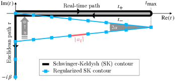
Figure 1: Schwinger-Keldysh (SK) contour (black) in the complex time plane and a regularized SK contour (blue) with tilt angle $\alpha$ and complex time step $a_{t}$. Both contours include a (tilted) real-time path and a Euclidean path.

All of these real-time observables can be extracted from unequal-time correlation functions. In practical simulations, such quantities suffer from a numerical sign problem Gattringer and Langfeld (2016), as we exemplify by the correlation of an arbitrary time-dependent observable $O(t)$. Expressed as a path integral over all realizations of the field $A$,

$$\langle O(t)O(t^{\prime})\rangle=\frac{1}{Z}\int\mathcal{D}A\,e^{iS[A]}O(t)O(t^{\prime}),$$ (1)

the correlator involves a complex-valued weight $\exp(iS)$. The highly oscillatory nature of this integral impedes the numerical application of standard Monte Carlo techniques. This becomes particularly hard in Minkowski space-time since the action $S[A]$ is real-valued.

Even though the sign problem has evaded a general and efficient solution due to its NP-hardness Troyer and Wiese (2005), progress on extracting observables can be made for individual systems nonetheless. Numerical simulations of real-time scalar fields have been carried out recently using the functional renormalization group Pawlowski and Strodthoff (2015); Huelsmann et al. (2020); Roth and von Smekal (2023) and contour deformation Alexandru et al. (2016, 2017). For QCD, transport coefficients and spectral functions have been computed using spectral reconstruction and analytic continuation in Euclidean lattice gauge theory Asakawa et al. (2001); Meyer (2008); Burnier et al. (2015); Altenkort et al. (2023a); Rothkopf (2022); Altenkort et al. (2023b), which forms an ill-posed inverse problem. Consequently, extracting accurate results becomes computationally challenging. Interesting alternative approaches employ analog and digital quantum simulators of gauge theories Zohar et al. (2016); Martinez et al. (2016); Bañuls et al. (2020), which are currently limited in their complexity and lattice size.

In this letter, we employ instead a stabilized version of the complex Langevin method to evade the sign problem. We achieve the first stable ab-initio computation of gauge-invariant real-time correlation functions in thermal SU(2) lattice gauge theory in 3+1 dimensions. This represents a breakthrough paving the way to extract transport coefficients and spectral functions directly.

Complex Langevin (CL) method – The CL approach is based on stochastic quantization Parisi and Wu (1981). In this method, the path integral expression in Eq. (1) is substituted by an average over a stochastic process for the fields. Although stochastic quantization was originally proposed for real-valued weights $\exp(-S)$, it was soon extended to the complex case, which is known as the complex Langevin (CL) method Parisi (1983). For Eq. (1), the stochastic process of gauge fields is described by

$$\frac{\partial}{\partial\theta}A^{a}_{\mu}(x,\theta)=\left.i\frac{\delta S}{\delta A^{a}_{\mu}(x)}\right\rvert_{\theta}+\eta^{a}_{\mu}(x,\theta),$$ (2)

where $x$ denotes the space-time point, $\theta$ the fictitious Langevin time and $\eta^{a}_{\mu}(x,\theta)$ is a real-valued Gaussian random field. The stationary limit $\theta\rightarrow\infty$ of the process $A^{a}_{\mu}(x,\theta)$ can be used to approximate the path integral. While issues with stability and wrong convergence can occur, important conceptual improvements including convergence criteria Aarts et al. (2010a); Nagata et al. (2016a); Kades et al. (2022) and numerical achievements have reinvigorated the field more recently. Adaptive Aarts et al. (2010b); Flower et al. (1986) and implicit Alvestad et al. (2021) solvers for the CL equation have been shown to lessen problems associated with unstable runaway trajectories. For gauge theories, convergence properties have been improved by gauge cooling Seiler et al. (2013), which exploits the gauge freedom of the CL process. In the realm of QCD at finite chemical potential, gauge cooling partially in combination with dynamical stabilization Attanasio and Jäger (2019) has led to advances in the computation of the equation of state Bongiovanni et al. (2014); Sexty (2014); Mollgaard and Splittorff (2013); Fodor et al. (2015); Nagata et al. (2016b); Aarts et al. (2016); Kogut and Sinclair (2019); Attanasio et al. (2020, 2022). Recently, there has been renewed interest in kernels Okamoto et al. (1989); Okano et al. (1991). Machine-learning-based kernels have been successfully applied to real-time scalar fields in up to 1+1 dimensions Alvestad et al. (2022); Lampl and Sexty (2023); Alvestad et al. (2023), which builds on previous results Berges and Stamatescu (2005); Berges et al. (2007); Alexandru et al. (2022). Further successful applications of the CL method include quantum many-body, cold atom, and spin systems Aarts and James (2012); Rammelmüller et al. (2018); Berger et al. (2021); Heinen and Gasenzer (2023).

However, the application of the real-time CL method to non-Abelian gauge theories had been elusive Berges et al. (2007); Berges and Sexty (2008); Aarts et al. (2018). This has changed with our recent revision of the CL equation for non-Abelian gauge theories Boguslavski et al. (2023); Hotzy et al. (2023), which enables unprecedentedly stable simulations on complex time contours. Here we use this new approach to extract real-time correlation functions in Yang-Mills theory.

Theory and method – We consider real-time SU($N_{c}$) Yang-Mills theory in 3+1 dimensions in thermal equilibrium. Formally, this system can be described within the Schwinger-Keldysh (SK) formalism Schwinger (1961); Keldysh (1964), which puts the theory on a complex time contour $\mathscr{C}$ shown as the black curve in Fig. 1. The real part of the contour (real-time path) describes the extent up to $t_{\mathrm{max}}$ in physical Minkowski time with a forward ($t_{+}$) and backward ($t_{-}$) time path. In contrast, the Euclidean path follows the imaginary time axis ($\tau$) whose extent corresponds to the inverse temperature $\beta=1/T$. The SK contour enters the action,

$$S[A]=-\frac{1}{2g^{2}}\int_{\mathscr{C}}\mathrm{d}t\int\mathrm{d}^{3}x\,\mathrm{Tr}[F^{\mu\nu}F_{\mu\nu}],$$ (3)

with the field-strength tensor $F^{\mu\nu}$ and the coupling constant $g$. The SK contour is closed, which implies periodic boundary conditions for the field $A(t{=}-i\beta)=A(t{=}0)$.

To simulate this system, we use a standard lattice gauge theory formulation that guarantees gauge invariance by construction Wilson (1974): we discretize the gauge fields on a lattice of size $N_{t}\times N_{s}^{3}$ and introduce unitary link variables $U_{\mu}(x)\simeq\exp{\left[ia^{\mu}t^{a}A^{a}_{\mu}(x+\hat{\mu}/2\big{)}\right]}$ (no sum over $\mu$), where $\hat{\mu}$ is a unit vector, $a^{\mu}$ are the lattice spacings and $t^{a}$ are the generators of SU($N_{c}$). The lattice analogue of Eq. (3) is given by the Wilson action

$$S_{\mathrm{w}}=\frac{1}{g^{2}}\sum_{x,\mu\neq\nu}\rho_{\mu\nu}(x)\mathrm{Tr}\left[U_{\mu\nu}(x)-\mathbbm{1}\right],$$ (4)

with $U_{\mu\nu}(x)=U_{\mu}(x)\,U_{\nu}(x+\hat{\mu})\,U^{-1}_{\mu}(x+\hat{\nu})\,U^{-1}_{\nu}(x)$ and prefactors $\rho_{0i}(x)=-a_{s}/a_{t}(x)$, $\rho_{ij}(x)=a_{t}(x)/a_{s}$. The SK contour enters through the time-dependent temporal spacings $a_{t}(x)$, whereas the spatial lattice spacing $a_{s}$ is constant. Dimensionful results are given in units of $a_{s}$.

The discretized CL equation corresponding to (2) reads

$$U_{\mu}(x,\!\theta\!+\!\epsilon)=e^{it^{a}\!\left[i\epsilon\Gamma_{\!\mu}\!(x)\left.\frac{\delta S_{\mathrm{w}}}{\delta A^{a}_{\!\mu}\!(x)}\right|_{\theta}+\sqrt{\epsilon\Gamma_{\!\mu}\!(x)}\,\eta^{a}_{\mu}\!(x,\theta)\right]}U_{\mu}(x,\!\theta),$$ (5)

where $\epsilon$ represents the Langevin time step. The Gaussian noise field satisfies

$$\langle\eta^{a}_{\mu}(x,\theta)\rangle=0,~{}\,\langle\eta^{a}_{\mu}(x,\theta)\eta^{b}_{\nu}(y,\theta^{\prime})\rangle=2\delta_{\theta\theta^{\prime}}\delta_{xy}\delta^{ab}\delta_{\mu\nu}.$$ (6)

Note that the real-time part of the SK contour leads to a complex-valued drift term $i\delta S_{\mathrm{w}}/\delta A^{a}_{\mu}(x)$. This necessitates the generalization of gauge links from SU($N_{c}$) to SL($N_{c}$, $\mathbb{C}$) and the analytical continuation of the action.

In the CL approach, we have the freedom to introduce a kernel $\Gamma_{\mu}$ Okamoto et al. (1989); Okano et al. (1991). Such a modification of the CL equation leaves the stationary solution unchanged. In our simulation we employ

$$\Gamma_{0}(x)=a_{t}^{2}(x)/a_{s}^{2},\quad\Gamma_{i}(x)=1.$$ (7)

This is motivated by a time-contour parametrization applied to the CL equation and originally introduced by us in Boguslavski et al. (2023). We have demonstrated that in combination with gauge cooling, this kernel enhances the stability and convergence of our simulations systematically as the lattice anisotropy $a_{s}/|a_{t}|$ increases. An improved update step Ukawa and Fukugita (1985) is employed to mitigate systematic errors (see the Supplemental Material).

In our simulations, we iteratively solve the discretized CL equation. At sufficiently late Langevin times, the gauge links are distributed according to the desired stationary probability density. We ensure this by computing observables such as Wilson loops and comparing them to Euclidean results where applicable. Expectation values $\langle{O}\rangle$ are calculated by sampling uncorrelated gauge configurations $\{U^{(i)}\}$

$$\langle{O}\rangle\approx\frac{1}{N_{\mathrm{cfgs}}}\sum_{i}^{N_{\mathrm{cfgs}}}{O}\big{[}U^{(i)}\big{]}.$$ (8)

To further validate our simulations, we calculate the unitarity norm in the Supplemental Material. We find that it assumes small, stable values, which have been empirically associated with the correct convergence of CL Seiler et al. (2013).

We regulate the path integral (1) by introducing a tilt angle $\alpha>0$ for the real-time part of the contour, as depicted in Fig. 1. This angle additionally softens the sign problem. While the discretized path integral for $\alpha=0$ is ill-defined Matsumoto (2022), the SK contour is reached in the limit $\alpha\rightarrow 0^{+}$. In our approach, we generate configurations for multiple tilt angles, compute expectation values $\langle O\rangle_{\alpha}$ and obtain real-time observables in the $\alpha\rightarrow 0$ limit,

$$\langle O\rangle=\lim_{\alpha\rightarrow 0^{+}}\langle O\rangle_{\alpha}.$$ (9)

We illustrate this extrapolation in Fig. 1. The grey arrow symbolizes the convergence of the tilted regularized contour (blue) toward the SK contour (black).

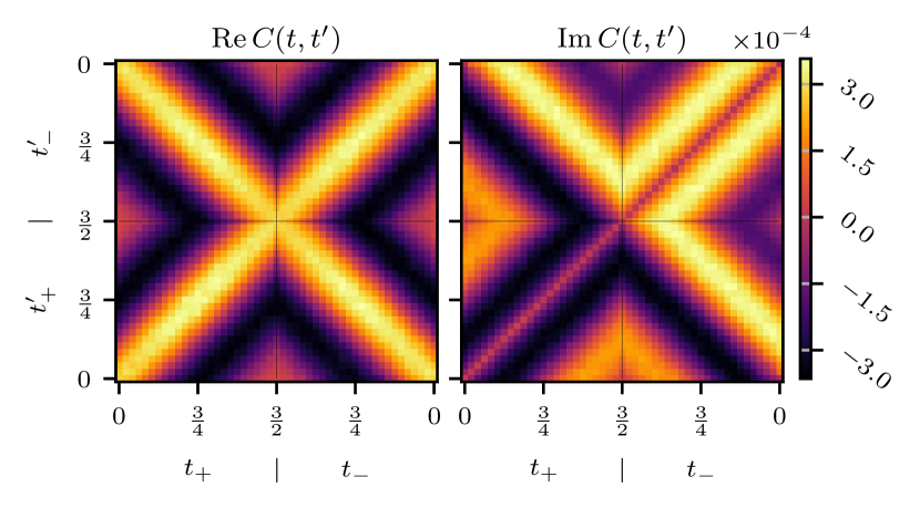
Figure 2: Real part (left) and imaginary part (right) of the unequal-time correlation function $C(t,t^{\prime})$ extrapolated onto the Schwinger-Keldysh contour using a cubic polynomial in $\alpha$. Forward and backward paths are indicated by $t_{\pm}$.

Correlations – An important class of observables accessible in real-time simulations of lattice gauge theory are unequal time correlation functions of the energy-momentum tensor

$$C_{\mu\nu;\rho\sigma}(t,\mathbf{x};t^{\prime},\mathbf{x}^{\prime})=\langle T_{\mu\nu}(t,\mathbf{x})T_{\rho\sigma}(t^{\prime},\mathbf{x}^{\prime})\rangle,$$ (10)

with $T_{\mu\nu}=2\mathrm{Tr}[F_{\mu}{}^{\alpha}F_{\alpha\nu}+\frac{1}{4}g_{\mu\nu}F_{\alpha\beta}F^{\alpha\beta}]$. The spectral function associated with Eq. (10) contains information about the transport properties of the system. In particular, $C_{\mu\mu;\nu\nu}$ and $C_{xy;xy}$ encode the bulk and shear viscosities $\eta$ and $\zeta$ entering hydrodynamic equations Romatschke and Romatschke (2019).

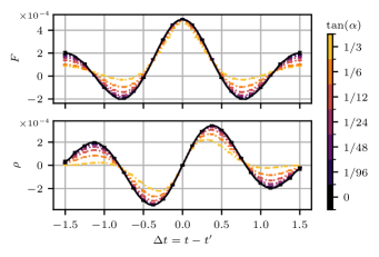
Figure 3: Statistical correlation function $F$ and spectral function $\rho$ as functions of the real-time difference $\Delta t=t-t^{\prime}$ for varying tilt angles $\alpha$. For finite $\alpha$, the real times $t,t^{\prime}$ are obtained by projecting the tilted time contour onto the real-time axis. The data extrapolates toward $\alpha\to 0$, indicating a clear convergence to finite real-time observables.

In this work, we focus on the magnetic contribution to the energy density calculated in terms of cloverleaves (see Supplemental Material)

$$O(t,\mathbf{x})=\frac{1}{2}\mathrm{Tr}[F_{ij}(t,\mathbf{x})F^{ij}(t,\mathbf{x})],$$ (11)

and the corresponding unequal-time correlator (cf., (1))

$$\!\!\!C(t,\!\mathbf{x};t^{\prime},\!\mathbf{x}^{\prime})\! =\!\langle O(t,\!\mathbf{x})O(t^{\prime},\!\mathbf{x}^{\prime})\rangle\!-\!\langle O(t,\!\mathbf{x})\rangle\langle O(t^{\prime},\!\mathbf{x}^{\prime})\rangle,$$ (12)

$$C(t,t^{\prime}) =\frac{1}{N_{s}^{3}}\sum_{\mathbf{x}}C(t,\mathbf{x};t^{\prime},\mathbf{x}).$$ (13)

The main advantage of studying $C(t,t^{\prime})$ is its close relation to the correlator of the energy-momentum tensor (10), while requiring fewer configurations due to the average over the spatial lattice sites $\mathbf{x}$. Nonetheless, $C(t,t^{\prime})$ has many non-trivial features that are common to such correlators in the SK limit $\alpha\rightarrow 0^{+}$, many of which we will explicitly check numerically.

Numerical setup – We simulate SU(2) gauge theory in thermal equilibrium on a lattice with $N_{s}^{3}=16^{3}$ spatial lattice points. The number of temporal lattice points $N_{t}$ is chosen to maintain a constant anisotropy $a_{s}/|a_{t}|\approx 16$ along the entire regularized complex time contour (Fig. 1), while decreasing the tilt angle $\tan(\alpha)=1/3\rightarrow 1/96$. We employ the bare coupling $g=0.5$, the inverse temperature $\beta=1/T=1$, and a maximal real-time extent of $t_{\mathrm{max}}=1.5\beta$. Following indications of our previous study on complex time contours Boguslavski et al. (2023), we note that both $t_{\mathrm{max}}$ and $g$ can be in principle increased systematically by using a finer temporal discretization, albeit at a higher computational cost.

In addition to the kernel in Eq. (7), we apply gauge cooling Seiler et al. (2013) with one cooling step after each update, using a step size $\alpha_{\mathrm{GC}}=0.05$, to stabilize our simulations (see Boguslavski et al. (2023) for details). The simulations start cold with unit matrices $U_{x,\mu}(\theta\!=\!0)=\mathbbm{1}$ and evolve with a constant Langevin time step $\epsilon=10^{-4}$. Field configurations for the measurement of observables are extracted within $10\leq\theta\leq 20$ after thermalization at Langevin times separated by $\Delta\theta=0.1$, which is well above the auto-correlation time of $O$. We also average over configurations generated from 100 to 1000 independent simulations. Error bars in the presented figures are determined using a bias-corrected jackknife method.

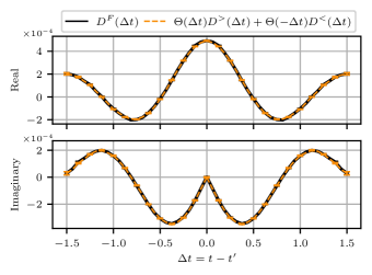
Figure 4: Relation between Feynman propagator and Wightman functions extracted independently from different quadrants of $C(t,t^{\prime})$ in Fig. 2. The top and bottom panels show real and imaginary parts of Eq. (17), respectively. Our simulations demonstrate that this consistency relation is satisfied with remarkable accuracy.

Extrapolated unequal-time correlator – We present our main result in Fig. 2, which shows the correlation function $C(t,t^{\prime})$ extrapolated to $\alpha\rightarrow 0^{+}$ and restricted to the real-time forward and backward paths. A striking feature of Fig. 2 is that $C(t,t^{\prime})$ splits into four distinct quadrants, where each quadrant represents a propagator,

$$D^{<}(t,t^{\prime})=C(t_{+},t_{-}^{\prime}), D^{\bar{F}}(t,t^{\prime})=C(t_{-},t_{-}^{\prime}),$$ (14)

$$D^{F}(t,t^{\prime})=C(t_{+},t_{+}^{\prime}), D^{>}(t,t^{\prime})=C(t_{-},t_{+}^{\prime}),$$

and $t$ is either $t_{+}$ or $t_{-}$, and similarly for $t^{\prime}$. Here $D^{F}$ and $D^{\bar{F}}$ are known as (anti-)Feynman propagators, and $D^{>}$ and $D^{<}$ are Wightman functions. Additionally, we see that $C(t,t^{\prime})$ exhibits a symmetry: in each quadrant, we find that the propagators become independent of the central time coordinate $\bar{t}=(t+t^{\prime})/2$:

$$D(t,t^{\prime})=D(t-t^{\prime})\equiv D(\Delta t).$$ (15)

This symmetric structure of $C(t,t^{\prime})$ is a direct consequence of time translation invariance in thermal equilibrium and only appears in the SK limit $\alpha\rightarrow 0^{+}$ (see our Supplemental Material for more details).

In Fig. 3, we present results for the statistical correlation function and the spectral function

$$F=\mathrm{Re}\,D^{F},~{}~{}\rho=-\mathrm{sgn}(\Delta t)\,\mathrm{Im}\,D^{F},$$ (16)

at various tilt angles of the discretized time contour, with signum function $\mathrm{sgn}(\Delta t)$. As the tilt angle decreases, both $F$ and $\rho$ approach the $\alpha\to 0^{+}$ extrapolated correlations (black curves). Consequently, we obtain finite values for these magnetic energy density correlators.

Consistency among propagators – There are well-established relations in field theory for different correlation functions. Analytically, the Feynman propagator can be expressed in terms of Wightman functions Ghiglieri et al. (2020)

$$D^{F}(t,t^{\prime})=\Theta(t\!-\!t^{\prime})D^{>}(t,t^{\prime})\!+\!\Theta(t^{\prime}\!-\!t)D^{<}(t,t^{\prime}),$$ (17)

where $\Theta(t{-}t^{\prime})$ is the Heaviside step function. With our approach, we can reproduce this correspondence numerically. In Fig. 4 we show that in the limit $\alpha\to 0^{+}$, Equation (17) is indeed satisfied. Furthermore, we emphasize that similarly to the emergence of the time translation invariance, Eq. (17) is not satisfied for finite tilt angles, but only after the extrapolation. This is shown in the Supplemental Material. Hence, the numerical consistency among different correlation functions turns out to be a non-trivial property manifest in the real-time evolution.

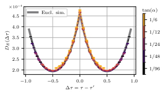
Figure 5: Euclidean correlator $D_{E}$ at different tilt angles. Remarkably, for the tilt angles $\alpha\leq\arctan(1/12)$, the Euclidean correlation aligns well with the Euclidean simulation result denoted by “Eucl. sim.”. The small deviations stem from statistical errors and minor differences in the lattice spacing.

Euclidean correlator – Since our system is formulated on the SK contour, our simulations also give us access to the Euclidean correlator

$$D_{E}(\tau,\tau^{\prime})=C(\tau,\tau^{\prime}),$$ (18)

where $\tau$ and $\tau^{\prime}$ are restricted to the imaginary Euclidean path of the contour (Fig. 1). Our results are shown in Fig. 5, where we present $D_{E}$ for various values of the tilt angle $\alpha$ and compare these correlators to the result of a Euclidean simulation, where no sign problem is present. We find remarkable agreement for a wide range of $\alpha$, showing the consistency of our simulations on the SK contour. We emphasize that due to the non-locality in Euclidean time, this result is significantly more robust to indicate correct convergence than the comparisons conducted in Berges et al. (2007); Boguslavski et al. (2023) where only time-translation invariant one-point functions have been used.

Conclusion – We have performed the first direct computation of unequal-time correlation functions in 3+1 dimensional real-time Yang-Mills theory in thermal equilibrium. These results are achieved by utilizing the complex Langevin method that we revised for complex time contours in Boguslavski et al. (2023) and applied here to the Schwinger-Keldysh (SK) contour using a polynomial extrapolation.

We have found that our new setup allows us to reliably extract real-time observables, as demonstrated by the correlation function of the magnetic contribution to the energy density. An important result is that the extracted correlators on the SK contour satisfy numerically non-trivial consistency relations that connect Wightman and Feynman propagators and are time-translation invariant. In contrast, such properties are violated on other complex time contours. Moreover, we have verified that our Euclidean correlator along the thermal path of the SK contour agrees with independent simulations using a traditional Monte Carlo method.

These results give a strong indication that our method can be extended to other gauge-invariant observables such as correlations of the energy-momentum tensor $T_{\mu\nu}$ or other transport coefficients for heavy quarks and jets. The generalization to SU(3) is straightforward, while simulations at larger couplings $g$ may be computationally more involved. More generally, our method can provide the means to access the spectral functions of various operators. So far, their direct non-perturbative real-time computation in gauge theories can be performed in classical-statistical lattice simulations Boguslavski et al. (2018, 2020, 2021, 2022); Ipp et al. (2020a, b); Avramescu et al. (2023), which are justified far from equilibrium at weak couplings and large occupancies. To avoid these underlying approximations, another exciting prospect of our framework is the simulation of gauge theories outside of thermal equilibrium. This would improve our understanding of the thermalization process of gauge theories, which has significant phenomenological consequences, particularly in the context of the pre-equilibrium phase of heavy-ion collisions.

In this Supplemental Material, we provide additional technical details on the improved Langevin step and the cloverleaf formulation of the magnetic energy density employed in our simulations. We further conduct numerical checks, including the unitarity norm, an emerging time-translation invariance, and consistency checks among propagators.

Improved Langevin step

In our Complex Langevin (CL) simulations, we utilize an improved update scheme that replaces Eq. (5) of the main text. This improves the convergence of the algorithm and alleviates systematic errors stemming from a finite Langevin step size Ukawa and Fukugita (1985); Fukugita et al. (1987). The update step reads

$$U_{\mu}(x,\theta+\epsilon)=e^{i\gamma t^{a}\left[i\epsilon\Gamma_{\mu}\widetilde{\frac{\delta S_{\mathrm{w}}}{\delta A^{a}_{\mu}}}+\sqrt{\epsilon\Gamma_{\mu}}\,\eta^{a}_{\mu}(x,\theta)\right]}U_{\mu}(x,\theta),$$ (19)

with $\gamma=1+\epsilon\,C_{A}/6$ and the quadratic Casimir $C_{A}=2$ for $\mathrm{SU}(2)$. The effective drift term is given by

$$\widetilde{\frac{\delta S_{\mathrm{w}}}{\delta A^{a}_{\mu}}}=\frac{1}{2}\left(\frac{\delta S_{\mathrm{w}}}{\delta A^{a}_{\mu}}\Big{[}U\Big{]}+\frac{\delta S_{\mathrm{w}}}{\delta A^{a}_{\mu}}\Big{[}\widetilde{U}\Big{]}\right),$$ (20)

and averages the usual drift at Langevin time $\theta$ (denoted by links $U$) with an auxiliary drift with links

$$\widetilde{U}_{\mu}(x,\theta\!+\!\epsilon)=e^{it^{a}\left[i\epsilon\Gamma_{\mu}\frac{\delta S_{\mathrm{w}}}{\delta A^{a}_{\mu}}[U]+\sqrt{\epsilon\Gamma_{\mu}}\,\eta^{a}_{\mu}(x,\theta)\right]}U_{\mu}(x,\theta).$$ (21)

The noise correlator is altered to

$$\langle\eta^{a}_{\mu}(x,\theta)\eta^{b}_{\nu}(y,\theta^{\prime})\rangle=2(1-\epsilon\,C_{A}/2)\,\delta_{\theta\theta^{\prime}}\delta_{xy}\delta^{ab}\delta_{\mu\nu}.$$ (22)

This procedure may be understood as a second-order Runge-Kutta-Munthe-Kaas solver for differentiable Lie groups Munthe-Kaas (1998), adapted for stochastic differential equations.

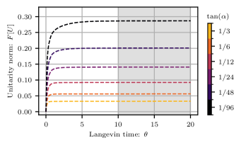
Figure 6: Unitarity norm $F[U]$ in (23) as a function of the Langevin time $\theta$ for different tilt angles of the simulated tilted time contour. As the tilt angle decreases, higher levels of non-unitarity are observed. Crucially, after a quick initial growth, all simulations lead to a plateau of the unitarity norm. The area highlighted by the grey background indicates where observables are measured.

Unitarity norm

Empirical observations have shown that the stability of the CL evolution is closely associated with the “non-unitarity” of the field configuration Seiler et al. (2013). This property is typically quantified by the unitarity norm

$$F[U]=\frac{1}{4N_{t}N_{s}^{3}}\sum_{x,\mu}\mathrm{Tr}\left[(U_{\mu}(x)U_{\mu}^{\dagger}(x)-\mathbbm{1})^{2}\right],$$ (23)

where $U_{\mu}(x)\in\mathrm{SL(N_{c},\mathbb{C})}$ denote the link variables. Unitary link configurations have a vanishing unitarity norm $F[U]=0$.

In all simulations, we initialize the field with identity matrices $U_{\mu}(x,\theta{=}0)=\mathbbm{1}$, thereby starting at $F[U]=0$. Figure 6 shows the unitarity with respect to Langevin time, averaged over all runs that we used to evaluate the correlation function. We observe that reducing the tilt angle leads to an increase in $F[U]$, indicating a more challenging sign problem. Crucially, however, the unitarity norm reaches a plateau after the thermalization of the complex Langevin process for all tilt angles. This suggests that the application of the anisotropic kernel in conjunction with the gauge cooling procedure successfully stabilizes the simulations. Observables are measured when the plateau is reached, and thermalization can be assumed. This region, $10\leq\theta\leq 20$, is highlighted by the grey band in Fig. 6.

Cloverleaf definition of the magnetic energy density

On the lattice, we obtain the field-strength tensor by relating it to the plaquette variable

$$U_{\mu\nu}(x)=\exp\left[ia_{\mu}a_{\nu}F_{\mu\nu}(x)+\mathcal{O}(a^{3})\right].$$ (24)

This allows us to determine the magnetic contribution to the energy density as

$$O(t,\mathbf{x}) =\frac{1}{2}\,\mathrm{Tr}[F_{ij}(t,\mathbf{x})F^{ij}(t,\mathbf{x})]$$

$$\approx-\sum_{i<j}\frac{1}{a_{i}^{2}a_{j}^{2}}\,\mathrm{Tr}\left\{\mathcal{P}_{A}(C_{ij}(x))^{2}\right\},$$ (25)

with

$$\mathcal{P}_{A}(C)\equiv\frac{1}{2}\left(C-C^{-1}-\frac{1}{N_{c}}\mathrm{Tr}\left(C-C^{-1}\right)\right).$$ (26)

For an $\mathrm{SU}(N_{c})$ matrix, this expression reduces to the anti-hermitian trace-zero part of $C$. The cloverleaf $C_{\mu\nu}(x)$ is given by

$$\begin{split}C_{\mu\nu}(x)=\frac{1}{4}[&U_{\mu\nu}(x)+U_{\nu(-\mu)}(x)+\\ &U_{(-\mu)(-\nu)}(x)+U_{(-\nu)\mu}(x)]\end{split}$$ (27)

and forms an average of four neighboring plaquettes. In contrast to using the plaquettes themselves, this results in a quantity that is defined on the lattice site $x$ and reduces lattice artifacts Bilson-Thompson et al. (2003).

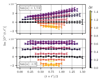
Figure 7: The imaginary part of the Wightman function $D^{>}$ is shown as a function of central time $(t+t^{\prime})/2$ for different fixed $\Delta t=t-t^{\prime}$ slices, indicated by different colors. The figure shows the correlation for a finite tilt angle $\tan(\alpha)=1/12$ (top) and the extrapolated correlation for $\tan(\alpha)\to 0$ (bottom). We stress that the time translation invariance is broken for finite tilt angles while it is satisfied for the extrapolated data.

Emergent time translation invariance

In thermal equilibrium, observables are time translation invariant. For one-point functions, this implies $\langle{O}(t)\rangle=\mathrm{const.}$ while two-point functions $\langle{O}(t){O}(t^{\prime})\rangle$ are independent of the central time $(t+t^{\prime})/2$ and only depend on the time difference $\Delta t\equiv t-t^{\prime}$. However, to obtain finite results in the lattice formulation, the real-time part of the path integral of the Schwinger-Keldysh contour requires regularization. As discussed in the main text, we introduce a tilt angle $\alpha$ to regularize the real-time part of the time contour. The time values are then extracted by projecting $t$ and $t^{\prime}$ onto the real-time axis. The tilt angle pulls apart different points on the forward and backward branches of the Schwinger-Keldysh contour for the same real times. This can effectively introduce an unphysical dependence on the central time for correlation functions, hence violating time translation invariance.

In Figure 7, we numerically confirm our expectations for the imaginary part of the Wightman function $D^{>}$. It shows the correlation function as a function of the central time $(t+t^{\prime})/2$ for varying time differences $\Delta t$, each represented by a different color. Horizontal lines in this representation indicate that the time translation invariance is intact. We observe that this feature is not present at the finite tilt angle $\tan(\alpha)=1/12$ shown in the top panel. When we extrapolate this correlator to the Schwinger-Keldysh contour $\alpha\to 0$, we find that the independence of the central time becomes well-preserved, as depicted in the bottom panel. A similar assertion holds for other correlation functions that we have calculated in this study; however, it is most pronounced in the case of the Wightman functions as they reflect correlations between forward and backward real-time branches. Additionally, we emphasize that not only the time independence is violated but also the values of the correlations are systematically distorted with respect to the central time.

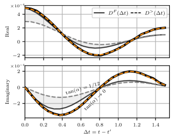
Figure 8: Comparison between Feynman propagator $D^{F}$ (continuous) and Wightman function $D^{>}$ (dashed) extracted independently from different sectors of the unequal-time correlator $C(t,t^{\prime})$. Data for the finite tilt angle $\tan(\alpha)=1/12$ is shown in grey and extrapolated data $\alpha\to 0$ in black and orange. The top and bottom panels show their real and imaginary parts, respectively. One observes that the non-trivial correspondence (28) between these correlations only emerges for $\alpha\to 0$.

Emergent consistency among propagators

We ensure the consistency and correctness of our results by explicitly checking well-established analytic relations of the correlators extracted from different real-time sectors of $C(t,t^{\prime})$. For $t>t^{\prime}$, the Feynman propagator in the $(t_{+},t_{+}^{\prime})$-sector should agree with the Wightman function $D^{>}$ extracted from the neighboring $(t_{-},t_{+}^{\prime})$-sector according to

$$D^{F}(t,t^{\prime})=\Theta(t\!-\!t^{\prime})D^{>}(t,t^{\prime})\!+\!\Theta(t^{\prime}\!-\!t)D^{<}(t,t^{\prime}).$$ (28)

In Fig. 8, we show the real and imaginary parts of this equation for $t>t^{\prime}$ for the extrapolated data with $\alpha\to 0$ and at finite, yet small, tilt angle $\tan(\alpha)=1/12$. For $\tan\alpha>0$ we also average over central times $(t+t^{\prime})/2$. Strikingly, the relation (28) is not satisfied for the latter, as indicated by the grey-shaded region that highlights the deviation between both correlators. It rather emerges in the limit $\alpha\to 0$, where the relation is satisfied to high accuracy. This underpins the necessity for the extrapolation procedure of our simulation strategy.