Resonant Spin-Flavor Precession of Sterile Neutrinos

Abstract

We analyze the impact of resonant conversions mediated by non-vanishing magnetic moments between active neutrinos and a heavy sterile neutrino on the supernova neutrino flux. We present the level-crossing scheme for such a scenario and derive the neutrino fluxes after conversion, paying particular attention to the order in which the resonances occur. We then compute the expected event rates from the neutronization burst of a future supernova at DUNE and Hyper-Kamiokande to derive new constraints on the neutrino magnetic moment. With this, we find a sensitivity down to a few ${10}^{-15}\text{\,}\mu_{\mathrm{B}}$ for a sterile neutrino in the $O($\text{\,}\mathrm{e}\mathrm{V}$)$ mass range.

Introduction

Shortly after the neutrino was first hypothesized by Pauli in 1930 [1], the first studies on the magnetic moment of the neutrino were already conducted, with a first experimental constraint established already in 1935 [2]. In recent years, the possibility of probing heavy sterile neutrinos through the magnetic moment has been intensely explored, with measurable effects ranging from terrestrial experiments, astrophysical phenomena, and cosmology [3, 4, 5].

In the present work, we revisit the resonant magnetic conversion, often called resonant spin-flavor precession (RSFP), of active neutrinos into sterile neutrinos inside a supernova, first investigated in ref. [6]. The mechanism is similar to magnetic transitions between active neutrinos [7, 8, 9, 10], and Mikheev-Smirnov-Wolfenstein (MSW) conversions between active and sterile neutrinos [11, 12, 13, 14], which have been studied extensively in the literature. These transitions can either convert part of the active neutrino flux into sterile neutrinos or, through successive transitions, change the flavors of the neutrinos as they propagate inside a supernova.

The structure of this paper is the following: in section 2 we formulate the basic ingredients for describing the magnetic conversion of active and sterile neutrinos. In section 3 we apply this formalism to a supernova environment and detail how the transitions at resonances affect the final fluxes. We then compare the expected rates of events with and without a magnetic moment at the future neutrino detectors DUNE and Hyper-Kamiokande in section 4. We summarize and discuss our results in section 5.

Neutrino Magnetic Moments

We consider a scenario where the Standard Model is extended by a right-handed singlet fermion $N$ of mass $M_{N}$, often called sterile neutrino or heavy neutral lepton, which couples to active neutrinos via a magnetic moment. These magnetic moment interactions are described by the effective operator

$$\mathcal{L}\supset\frac{\hat{\mu}_{\nu}^{\alpha N}}{2}F_{\mu\nu}\bar{\nu}_{\alpha}\sigma^{\mu\nu}N+\text{h.c.},$$ (1)

where $\nu^{\alpha}$ is the left-handed neutrino field of flavour $\alpha$, and $F_{\mu\nu}$ is the electromagnetic field strength tensor. In this work, we make no distinction between $N$ being a Majorana or a Dirac fermion. In principle, an important difference between the Dirac and Majorana cases is that, if $N$ were Majorana, one could have transitions $\nu_{L}\to N_{R}\to N_{R}^{c}\to\nu_{L}^{c}$, however the $N_{R}\to N_{R}^{c}$ oscillation is suppressed by a factor of $M_{N}^{2}/p^{2}$ [15, 16, 17, 18, 19], where $p$ is the momentum of $N$. Given that we only consider $M_{N}$ up to $\sim$10\text{\,}\mathrm{k}\mathrm{e}\mathrm{V}$$, and typical energies of supernova neutrinos are in the MeV range, this effect is negligible for the present work. The neutrino flavour eigenstate fields $\nu_{L}^{\alpha}$ are related to their mass eigenstates, $\nu^{i}$ as to

$$\nu_{\alpha}=U_{\alpha i}\nu_{i}\,,$$ (2)

where

$$U=\begin{pmatrix}1&&\\ &c_{23}&s_{23}\\ &-s_{23}&c_{23}\end{pmatrix}\!\!\!\begin{pmatrix}c_{13}&&s_{13}e^{i\delta}\\ &1&\\ -s_{13}e^{i\delta}&&c_{13}\end{pmatrix}\!\!\!\begin{pmatrix}c_{12}&s_{12}&\\ -s_{12}&c_{12}&\\ &&1\end{pmatrix}$$

is the Pontecorvo–Maki–Nakagawa–Sakata (PMNS) matrix, with $s_{ij}\equiv\sin\theta_{ij}$, $c_{ij}\equiv\cos\theta_{ij}$, and the CP-violating phase $\delta$.

The flavor evolution of a neutrino is governed by the Schrödinger equation

$$i\frac{\text{d}}{\text{d}t}\psi(t)=\hat{H}\psi(t)\,,$$ (3)

where $\psi$ is a unit vector in flavor space whose components describe the admixture of each flavor to the neutrino state. In the flavor basis, $\psi$ is given by $\psi=(\nu_{e},\nu_{\mu},\nu_{\tau},N)$ and we can write the Hamiltonian in block diagonal form as

$$\hat{H} =\frac{1}{2p}\begin{pmatrix}U&\\ &1\end{pmatrix}\begin{pmatrix}\hat{M}_{\nu}^{2}&\\ &M_{N}^{2}\end{pmatrix}\begin{pmatrix}U^{\dagger}&\\ &1\end{pmatrix}$$

$$+\begin{pmatrix}\hat{H}_{\text{MSW}}&\\ &0\end{pmatrix}+\frac{B_{\perp}}{2}\begin{pmatrix}0&\hat{\mu}_{\nu}\\ \hat{\mu}_{\nu}^{\dagger}&0\end{pmatrix}\,.$$ (4)

with the neutrino momentum $p$, the diagonal mass matrix

$$\hat{M}_{\nu}=\text{diag}(m_{\nu_{1}},m_{\nu_{2}},m_{\nu_{3}})\,,$$ (5)

the MSW potential

$$\hat{H}_{\text{MSW}}=\begin{pmatrix}V_{\nu_{e}}&&\\ &V_{\nu_{\mu}}&\\ &&V_{\nu_{\tau}}\end{pmatrix}\,,$$ (6)

and the magnetic moment vector

$$\hat{\mu}_{\nu}=\begin{pmatrix}\mu_{\nu}^{eN}\\ \mu_{\nu}^{\mu N}\\ \mu_{\nu}^{\tau N}\end{pmatrix}\,.$$ (7)

In principle, the perpendicular magnetic field $B_{\perp}$ also contains a geometric phase $\phi$ defined by $B_{x}+iB_{y}=B_{\perp}e^{i\phi}$, assuming $z$ is the propagation axis of the neutrinos. Variations of this geometric phase can alter the resonant behavior or give rise to new resonances [20, 21, 22]. The primary impact of this in our scenario would be a shift by $\dot{\phi}$ in the resonance condition [23], which in our case can be compensated by a shift in $M_{N}$ (s. section 3). Additionally, if $\ddot{\phi}$ is large, it can also decrease the adiabaticity parameter, leading to a weaker sensitivity. In the absence of precise estimates of both $\dot{\phi}$ and $\ddot{\phi}$, we don’t consider this effect in the present work.

We also note that the large mass gap between the active and the sterile neutrinos suppresses spin-flavor oscillations in vacuum, unlike in the Dirac case [24, 25, 26, 27, 28]. We further neglect mass mixing between the active neutrinos and $N$.

Assuming equal number densities of electrons and protons and defining the electron number fraction $Y_{e}=n_{e}/(n_{e}+n_{p})$, the MSW potentials can be written as

$$V_{\nu_{e}}= \frac{\sqrt{2}}{2}G_{F}\frac{\rho}{m_{N}}(3\,Y_{e}-1),$$ (8)

$$V_{\nu_{\mu,\tau}}= \frac{\sqrt{2}}{2}G_{F}\frac{\rho}{m_{N}}(Y_{e}-1),$$ (9)

where $G_{F}$ is the Fermi constant, $\rho$ is the matter density and $m_{N}$ the nucleon mass.

Neutrino Conversion inside the Supernova

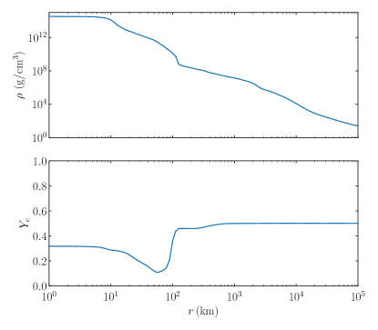
Figure 1: Density and electron fraction profiles for a $10.8M_{\astrosun}$ progenitor supernova at $t=$30\text{\,}\mathrm{m}\mathrm{s}$$ after core bounce, taken from ref. [29].

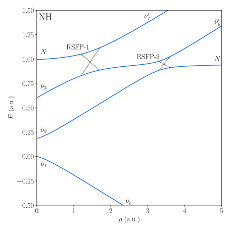
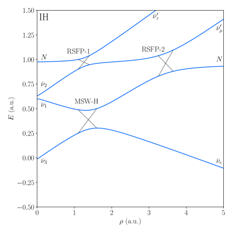
Figure 2: Level-crossing scheme for normal (left) and inverted (right) hierarchy, assuming $Y_{e}>1/3$.

In the current work, we analyze the neutrino flux during the neutronization burst, in which a large number of neutrinos are emitted in a short period of time. The predictions of the neutrino flux during this phase are consistent up to $O(10\%)$ among different simulations; in this work we use the initial flux from ref. [30] for a supernova with a $8.8\,M_{\astrosun}$ progenitor. We use the results from ref. [29] for a $10.8\,M_{\astrosun}$ progenitor at $30\text{\,}\mathrm{m}\mathrm{s}$ after bounce for the mass density and electron fraction profiles. In addition to this, we model the magnetic field within the supernova as a dipole $B(r)=2B_{0}r_{0}^{3}/(r^{3}+r_{0}^{3})$ [31], where $B_{0}$ is the magnetic field at the iron surface, and $r_{0}=$1671\text{\,}\mathrm{k}\mathrm{m}$$ is the radius of the iron core. Throughout this work we set $B_{0}=${10}^{12}\text{\,}\mathrm{G}$.$

There has been significant interest in magnetic fields of core-collapse supernovae in recent years, both due to their potential impact on the explosion mechanism and to explain the formation of highly magnetized neutron stars, so-called magnetars. In particular, recent magnetohydrodynamic simulations have found that initial magnetic fields of the order of ${10}^{12}\text{\,}\mathrm{G}$ can be amplified by up to three orders of magnitude via magnetorotational instabilities [32] as well as standing accretion shock instabilities [33] a few milliseconds after bounce.

As can be seen in fig. 1, $Y_{e}$ undergoes a significant change at $r\approx$100\text{\,}\mathrm{k}\mathrm{m}$$, going from initially $Y_{e}<1/3$ to $Y_{e}\approx 1/2$. This means that the electron and anti-electron neutrino mass potentials undergo a sign change at this point.

Since large potential differences damp transitions mediated by the magnetic moment, we only need to consider transitions at resonances, where energy differences are small. We find that, apart from the usual MSW resonances, in this scenario we have additional $\nu\leftrightarrow N$ resonances due to the magnetic moment, which can be computed in a two-flavor approximation.

The resonances occur when the instantaneous eigenvalues of the Hamiltonian are closest to one another; alternatively, for RSFP transitions, they occur where the eigenvalues cross when we turn the magnetic interactions off. In general, the precise resonance point depends on the masses and mixings of the neutrinos as well as the matter potentials; however, given that we generally assume $M_{N}\gg m_{\nu}$, the mass contributions to the Hamiltonian become negligible, and the resonance condition can be approximated as

$$V_{\nu_{e,\mu,\tau}}=\pm\frac{M_{N}^{2}}{2p}.$$ (10)

We define the adiabaticity parameter

$$\gamma_{\text{res}}=\left|\frac{8\mu_{\nu}^{2}B_{\perp}^{2}}{dV_{\nu}/dr}\right|,$$ (11)

with which we can estimate the transition probability at a resonance in the Landau-Zener approximation as

$$P_{\text{res}}\approx e^{-\frac{\pi}{2}\gamma_{\text{res}}},$$ (12)

where $\gamma_{\text{res}}$ is computed at the resonance point.

It is important to note that the conversions occur between instantaneous mass eigenstates and not flavor eigenstates. Therefore, in order to obtain the correct magnetic moments to be inserted into eq. 11, one needs to rotate the magnetic moment vector (7) into the appropriate basis. In doing so, we find that, even when assuming all neutrino flavors to have the same magnetic moment, the magnetic moments involved in each resonance can deviate by up to an order of magnitude from one another.

The level-crossing scheme for this scenario is shown in fig. 2. We order the resonances involving anti-neutrinos according to the densities at which they occur as RSFP-1, RSFP-2, and RSFP-3, while there is a single resonance involving neutrinos, which we call RSFP-E.

Assuming the MSW resonances are adiabatic, the fluxes in the mass eigenbasis for normal hierarchy upon leaving the supernova are

$$F_{\nu_{3}}= P_{E}F_{\nu_{e}}^{0},$$ (13a)

$$F_{\bar{\nu}_{1}}= P_{3}F_{\bar{\nu}_{e}}^{0},$$ (13b)

$$F_{\bar{\nu}_{2}}= P_{2}F_{\bar{\nu}^{\prime}_{\mu}}^{0}+(1-P_{3})(1-P_{2})F_{\bar{\nu}_{e}}^{0},$$ (13c)

$$F_{\bar{\nu}_{3}}= P_{1}F_{\bar{\nu}^{\prime}_{\tau}}^{0}+(1-P_{2})(1-P_{1})F_{\bar{\nu}^{\prime}_{\mu}}^{0}$$

$$+(1-P_{3})P_{2}(1-P_{1})F_{\bar{\nu}_{e}}^{0},$$ (13d)

while for inverted hierarchy, we find

$$F_{\nu_{2}}= P_{E}F_{\nu_{e}}^{0},$$ (14a)

$$F_{\bar{\nu}_{3}}= P_{3}F_{\bar{\nu}_{e}}^{0},$$ (14b)

$$F_{\bar{\nu}_{1}}= P_{2}F_{\bar{\nu}^{\prime}_{\tau}}^{0}+(1-P_{3}(1-P_{2})F_{\bar{\nu}_{e}}^{0},$$ (14c)

$$F_{\bar{\nu}_{2}}= P_{1}F_{\bar{\nu}^{\prime}_{\mu}}^{0}+(1-P_{2})(1-P_{1})F_{\bar{\nu}^{\prime}_{\tau}}^{0}$$

$$+(1-P_{3})P_{2}(1-P_{1})F_{\bar{\nu}_{e}}.$$ (14d)

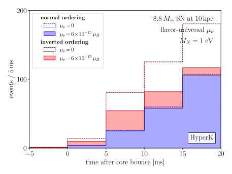
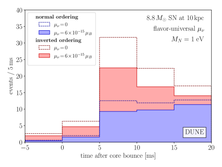
Figure 3: Comparison of rates at Hyper-K (left) and DUNE (right) for $\mu_{\nu}=0,$6\text{\times}{10}^{-15}\text{\,}\mu_{\mathrm{B}}$$, $B_{0}=${10}^{12}\text{\,}\mathrm{G}$$ and $M_{N}=$1\text{\,}\mathrm{e}\mathrm{V}$$ for normal and inverted orderings.

Sensitivity in Future Experiments

The transitions described in section 3 would alter the neutrino fluxes arriving at Earth and would therefore leave an imprint in neutrino detectors at Earth. In the present work, we consider the signal from the neutronisation burst of a supernova in two future detectors: Hyper-Kamiokande (HK) [34, 35], a $374\text{\,}\mathrm{k}\mathrm{t}$ water Cherenkov detector, and DUNE [36, 37], a $40\text{\,}\mathrm{k}\mathrm{t}$ liquid argon time projection chamber. HK mainly detects electron anti-neutrinos via inverse beta decay ($\bar{\nu}_{e}+p\to e^{+}+n$), while DUNE is most sensitive to $\nu_{e}$ via charged current scattering on argon ($\nu_{e}+{}^{40}\text{Ar}\to e^{-}+{}^{40}\text{K}^{*}$). Other detection channels considered are charged current scattering on oxygen ($\nu_{e}(\bar{\nu}_{e})+{}^{16}\text{O}\to e^{\pm}+X$) for HK, as well as neutral current elastic scattering on electrons ($\nu_{x}+e^{-}\to\nu_{x}+e^{-}$) for both. The cross-sections for these processes have been computed in refs. [38, 39, 40, 41, 42].

The fluxes of neutrinos of flavor $\alpha$ arriving at Earth are then given by

$$F_{\nu_{\alpha}}(E_{\nu})=\sum_{i}|U_{\alpha i}|^{2}F_{\nu_{i}}(E_{\nu}),$$ (15)

where $F_{\nu_{i}}$ is the flux of neutrinos in the mass eigenstate $i$ after conversion inside the supernova, following eqs. 13 and 14.

We split the signal into five equidistant time bins from $t=-$5\text{\,}\mathrm{m}\mathrm{s}$$ to $20\text{\,}\mathrm{m}\mathrm{s}$ with respect to the core bounce and perform a $\chi^{2}$ analysis comparing the hypotheses of zero versus finite neutrino magnetic moments. To do this, we define

$$\chi^{2}=\underset{a}{\text{min}}\sum_{i}\frac{n_{i}(\mu_{\nu},M_{N})-(1+a)n_{i}(0)}{(1+a)n_{i}(0)}+\frac{a^{2}}{\sigma_{a}^{2}},$$ (16)

where $n_{i}(\mu_{\nu},M_{N})$ is the expected number of events in bin $i$ for a magnetic moment $\mu_{\nu}$, while $n_{i}(0)$ is the number events for vanishing magnetic moment. We further introduce a nuisance parameter $a$ to parametrize the uncertainty in the normalization of the initial neutrino flux. We estimate the uncertainty as $\sigma_{a}=0.1$. Values of $\mu_{\nu}$ and $M_{N}$ for which $\chi^{2}$ is larger than $4.605$ can be excluded at the $90\%$ C.L. A comparison of the expected number of events both with and without a magnetic moment for $M_{N}=$1\text{\,}\mathrm{e}\mathrm{V}$$ and $\mu_{\nu}=$6\text{\times}{10}^{-15}\text{\,}\mu_{\mathrm{B}}$$ is shown in fig. 3.

Discussion and Conclusion

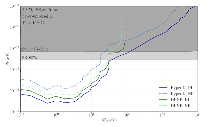
Figure 4: Projected sensitivities at $90\%$ confidence level. Limits for Hyper-Kamiokande are shown in shades of blue, while the ones for DUNE are in shades of green. We assume flavor-universal couplings, a distance of $10\text{\,}\mathrm{k}\mathrm{p}\mathrm{c}$ to the supernova, and set $B_{0}=${10}^{12}\text{\,}\mathrm{G}$$ at the iron surface of the progenitor star. Constraints from stellar cooling as well as from SN1987a (from [3] and [43] respectively) are shown in grey.

In the present work, we have revisited the impact of resonant magnetic transitions of active neutrinos into a heavy sterile state on supernova measurements. We have found that this method is sensitive to magnetic moments down to a few ${10}^{-15}\text{\,}\mu_{\mathrm{B}}$ for a sterile neutrino mass in the $O($\text{\,}\mathrm{e}\mathrm{V}$)$ range. The contours at $90\%$ confidence level assuming $B_{0}=${10}^{12}\text{\,}\mathrm{G}$$ at the iron surface for a supernova at $10\text{\,}\mathrm{k}\mathrm{p}\mathrm{c}$ are summarized in fig. 4. In principle, the constraints extend to $M_{N}$ below ${10}^{-1}\text{\,}\mathrm{e}\mathrm{V}$, but, in this region, $M_{N}$ and the active neutrino masses become comparable in size, and a more precise knowledge of the absolute neutrino masses as well as a careful treatment of the level-crossing scheme becomes necessary, which goes beyond the scope of this work.

Also shown in fig. 4 are constraints stemming from stellar cooling [43] as well as from SN1987a [3]. The idea behind them is that sterile neutrinos can be produced via the magnetic moment interaction from the hot plasma inside the stars and escape the star unhindered, increasing its cooling rate and altering its evolution.

A similar analysis to the one presented in this paper using SN1987a data was attempted by applying the same methods to the time-integrated flux. Since, however, the main effect of resonant magnetic conversion on supernova neutrino measurements is an overall deficit of the flux, and the total luminosity is a free parameter of the fit, we were unable to derive new constraints from it. We have not analyzed the time-dependent flux, but we don’t expect it to yield much better results.

We expect the strongest constraints to be found for $M_{N}$ at around $1\text{\,}\mathrm{e}\mathrm{V}$. In this case, the resonances happen at $r\approx r_{0}$, where the magnetic field is close to its maximum, and $dV/dr$ has already decreased considerably. It should be noted, however, that our constraints depend on the precise magnetic field of the supernova. Since the adiabaticity parameter depends on the product $\mu_{\nu}B$, the sensitivity in $\mu_{\nu}$ is inversely proportional to the magnetic field strength. In addition to this, while the first derivative of the geometric phase $\dot{\phi}$ only affects the resonance point and therefore shifts our curves in the $M_{N}$ axis, a large turbulent component to the magnetic field may compromise adiabatic conversion altogether if the second derivative of the geometric phase $\ddot{\phi}$ is much larger than $dV/dr$ [20].

While modeling the magnetic field of supernovae is still challenging, this field has been rapidly evolving, with studies investigating the emission of the SN1987a remnant to infer properties of its progenitor [44, 45, 46]. We believe that, by the time the next galactic supernova occurs, we will be able to better understand its magnetic field profile and, from this, derive concrete constraints on (or discover) large neutrino magnetic moments.

References

- Pauli [1978] W. Pauli, Dear radioactive ladies and gentlemen, Phys. Today 31N9, 27 (1978).
- Nahmias [1935] M. E. Nahmias, An Attempt to Detect the Neutrino, Math. Proc. Cambridge Phil. Soc. 31, 99 (1935).
- Magill et al. [2018] G. Magill, R. Plestid, M. Pospelov, and Y.-D. Tsai, Dipole Portal to Heavy Neutral Leptons, Phys. Rev. D 98, 115015 (2018), arXiv:1803.03262 [hep-ph] .
- Brdar et al. [2021] V. Brdar, A. Greljo, J. Kopp, and T. Opferkuch, The Neutrino Magnetic Moment Portal: Cosmology, Astrophysics, and Direct Detection, JCAP 01, 039, arXiv:2007.15563 [hep-ph] .
- Brdar et al. [2023] V. Brdar, A. de Gouvêa, Y.-Y. Li, and P. A. N. Machado, Neutrino magnetic moment portal and supernovae: New constraints and multimessenger opportunities, Phys. Rev. D 107, 073005 (2023), arXiv:2302.10965 [hep-ph] .
- Nunokawa et al. [1999] H. Nunokawa, R. Tomas, and J. W. F. Valle, Type II supernovae and neutrino magnetic moments, Astropart. Phys. 11, 317 (1999), arXiv:astro-ph/9811181 .
- Akhmedov [1988a] E. K. Akhmedov, Resonance enhancement of the neutrino spin precession in matter and the solar neutrino problem, Sov. J. Nucl. Phys. 48, 382 (1988a).
- Lim and Marciano [1988] C.-S. Lim and W. J. Marciano, Resonant Spin - Flavor Precession of Solar and Supernova Neutrinos, Phys. Rev. D 37, 1368 (1988).
- Akhmedov [1988b] E. K. Akhmedov, Resonant Amplification of Neutrino Spin Rotation in Matter and the Solar Neutrino Problem, Phys. Lett. B 213, 64 (1988b).
- Jana et al. [2022] S. Jana, Y. P. Porto-Silva, and M. Sen, Exploiting a future galactic supernova to probe neutrino magnetic moments, JCAP 09, 079, arXiv:2203.01950 [hep-ph] .
- Kainulainen et al. [1991] K. Kainulainen, J. Maalampi, and J. T. Peltoniemi, Inert neutrinos in supernovae, Nucl. Phys. B 358, 435 (1991).
- Raffelt and Sigl [1993] G. Raffelt and G. Sigl, Neutrino flavor conversion in a supernova core, Astropart. Phys. 1, 165 (1993), arXiv:astro-ph/9209005 .
- Shi and Sigl [1994] X. Shi and G. Sigl, A Type II supernovae constraint on electron-neutrino - sterile-neutrino mixing, Phys. Lett. B 323, 360 (1994), [Erratum: Phys.Lett.B 324, 516–516 (1994)], arXiv:hep-ph/9312247 .
- Argüelles et al. [2019] C. A. Argüelles, V. Brdar, and J. Kopp, Production of keV Sterile Neutrinos in Supernovae: New Constraints and Gamma Ray Observables, Phys. Rev. D 99, 043012 (2019), arXiv:1605.00654 [hep-ph] .
- Bahcall and Primakoff [1978] J. N. Bahcall and H. Primakoff, Neutrino-anti-neutrinos Oscillations, Phys. Rev. D 18, 3463 (1978).
- Schechter and Valle [1981] J. Schechter and J. W. F. Valle, Neutrino Oscillation Thought Experiment, Phys. Rev. D 23, 1666 (1981).
- Li and Wilczek [1982] L. F. Li and F. Wilczek, PHYSICAL PROCESSES INVOLVING MAJORANA NEUTRINOS, Phys. Rev. D 25, 143 (1982).
- Bernabeu and Pascual [1983] J. Bernabeu and P. Pascual, CP Properties of the Leptonic Sector for Majorana Neutrinos, Nucl. Phys. B 228, 21 (1983).
- Kimura and Takamura [2021] K. Kimura and A. Takamura, Unification of Neutrino-Neutrino and Neutrino-Antineutrino Oscillations (2021), arXiv:2101.04509 [hep-ph] .
- Smirnov [1991] A. Y. Smirnov, The Geometrical phase in neutrino spin precession and the solar neutrino problem, Phys. Lett. B 260, 161 (1991).
- Akhmedov et al. [1991] E. K. Akhmedov, A. Y. Smirnov, and P. I. Krastev, Resonant neutrino spin flip transitions in twisting magnetic fields, Z. Phys. C 52, 701 (1991).
- Balantekin and Loreti [1993] A. B. Balantekin and F. Loreti, Consequences of twisting solar magnetic fields in solar neutrino experiments, Phys. Rev. D 48, 5496 (1993).
- Jana and Porto [2023] S. Jana and Y. Porto, New Resonances of Supernova Neutrinos in Twisting Magnetic Fields (2023), arXiv:2303.13572 [hep-ph] .
- Kurashvili et al. [2017] P. Kurashvili, K. A. Kouzakov, L. Chotorlishvili, and A. I. Studenikin, Spin-flavor oscillations of ultrahigh-energy cosmic neutrinos in interstellar space: The role of neutrino magnetic moments, Phys. Rev. D 96, 103017 (2017), arXiv:1711.04303 [hep-ph] .
- Lichkunov et al. [2022] A. Lichkunov, A. Popov, and A. Studenikin, Three-flavour neutrino oscillations in a magnetic field (2022), arXiv:2207.12285 [hep-ph] .
- Alok et al. [2023a] A. K. Alok, N. R. Singh Chundawat, and A. Mandal, Cosmic neutrino flux and spin flavor oscillations in intergalactic medium, Phys. Lett. B 839, 137791 (2023a), arXiv:2207.13034 [hep-ph] .
- Kopp et al. [2022] J. Kopp, T. Opferkuch, and E. Wang, Magnetic Moments of Astrophysical Neutrinos (2022), arXiv:2212.11287 [hep-ph] .
- Alok et al. [2023b] A. K. Alok, T. J. Chall, N. R. S. Chundawat, and A. Mandal, Spin-Flavor Oscillations of Relic Neutrinos in Primordial Magnetic Field (2023b), arXiv:2311.04087 [hep-ph] .
- Fischer et al. [2010] T. Fischer, S. C. Whitehouse, A. Mezzacappa, F. K. Thielemann, and M. Liebendorfer, Protoneutron star evolution and the neutrino driven wind in general relativistic neutrino radiation hydrodynamics simulations, Astron. Astrophys. 517, A80 (2010), arXiv:0908.1871 [astro-ph.HE] .
- Hudepohl et al. [2010] L. Hudepohl, B. Muller, H. T. Janka, A. Marek, and G. G. Raffelt, Neutrino Signal of Electron-Capture Supernovae from Core Collapse to Cooling, Phys. Rev. Lett. 104, 251101 (2010), [Erratum: Phys.Rev.Lett. 105, 249901 (2010)], arXiv:0912.0260 [astro-ph.SR] .
- Suwa et al. [2007] Y. Suwa, T. Takiwaki, K. Kotake, and K. Sato, Magnetorotational Collapse of Population III Stars, Publ. Astron. Soc. Jap. 59, 771 (2007), arXiv:0704.1945 [astro-ph] .
- Rembiasz et al. [2016] T. Rembiasz, J. Guilet, M. Obergaulinger, P. Cerdá-Durán, M. A. Aloy, and E. Müller, On the maximum magnetic field amplification by the magnetorotational instability in core-collapse supernovae, Monthly Notices of the Royal Astronomical Society 460, 3316–3334 (2016).
- Varma et al. [2022] V. Varma, B. Mueller, and F. R. N. Schneider, 3D simulations of strongly magnetized non-rotating supernovae: explosion dynamics and remnant properties, Mon. Not. Roy. Astron. Soc. 518, 3622 (2022), arXiv:2204.11009 [astro-ph.HE] .
- Lagoda [2017] J. Lagoda, The Hyper-Kamiokande Project, PoS FPCP2017, 024 (2017), slides available from https://indico.cern.ch/event/586719/contributions/2531379/.
- Abe et al. [2018] K. Abe et al. (Hyper-Kamiokande), Hyper-Kamiokande Design Report (2018), arXiv:1805.04163 [physics.ins-det] .
- Abi et al. [2020a] B. Abi et al. (DUNE), Deep Underground Neutrino Experiment (DUNE), Far Detector Technical Design Report, Volume II DUNE Physics (2020a), arXiv:2002.03005 [hep-ex] .
- Abi et al. [2020b] B. Abi et al. (DUNE), Supernova Neutrino Burst Detection with the Deep Underground Neutrino Experiment (2020b), arXiv:2008.06647 [hep-ex] .
- Gil Botella and Rubbia [2003] I. Gil Botella and A. Rubbia, Oscillation effects on supernova neutrino rates and spectra and detection of the shock breakout in a liquid argon TPC, JCAP 10, 009, arXiv:hep-ph/0307244 .
- Strumia and Vissani [2003] A. Strumia and F. Vissani, Precise quasielastic neutrino/nucleon cross-section, Phys. Lett. B 564, 42 (2003), arXiv:astro-ph/0302055 .
- Nakazato et al. [2018] K. Nakazato, T. Suzuki, and M. Sakuda, Charged-current scattering off 16O nucleus as a detection channel for supernova neutrinos, PTEP 2018, 123E02 (2018), arXiv:1809.08398 [astro-ph.HE] .
- Bahcall et al. [1995] J. N. Bahcall, M. Kamionkowski, and A. Sirlin, Solar neutrinos: Radiative corrections in neutrino - electron scattering experiments, Phys. Rev. D 51, 6146 (1995), arXiv:astro-ph/9502003 .
- Ricciardi et al. [2022] G. Ricciardi, N. Vignaroli, and F. Vissani, An accurate evaluation of electron (anti-)neutrino scattering on nucleons, JHEP 08, 212, arXiv:2206.05567 [hep-ph] .
- Capozzi and Raffelt [2020] F. Capozzi and G. Raffelt, Axion and neutrino bounds improved with new calibrations of the tip of the red-giant branch using geometric distance determinations, Phys. Rev. D 102, 083007 (2020), arXiv:2007.03694 [astro-ph.SR] .
- Orlando et al. [2015] S. Orlando, M. Miceli, M. L. Pumo, and F. Bocchino, Supernova 1987A: a Template to Link Supernovae to their Remnants, Astrophys. J. 810, 168 (2015), arXiv:1508.02275 [astro-ph.HE] .
- Orlando et al. [2019] S. Orlando et al., 3D MHD modeling of the expanding remnant of SN 1987A. Role of magnetic field and non-thermal radio emission, Astron. Astrophys. 622, A73 (2019), arXiv:1812.00021 [astro-ph.HE] .
- Petruk et al. [2022] O. Petruk, V. Beshley, S. Orlando, F. Bocchino, M. Miceli, S. Nagataki, M. Ono, S. Loru, A. Pellizzoni, and E. Egron, Polarized radio emission unveils the structure of the pre-supernova circumstellar magnetic field and the radio emission in SN1987A, Mon. Not. Roy. Astron. Soc. 518, 6377 (2022), arXiv:2212.00656 [astro-ph.HE] .