Modelling molecular clouds and CO excitation in AGN-host galaxies

Abstract

We present a new physically-motivated model for estimating the molecular line emission in active galaxies. The model takes into account (i) the internal density structure of giant molecular clouds (GMCs), (ii) the heating associated both to stars and to the active galactic nuclei (AGN), respectively producing photodissociation regions (PDRs) and X-ray dominated regions (XDRs) within the GMCs, and (iii) the mass distribution of GMCs within the galaxy volume. The model needs, as input parameters, the radial profiles of molecular mass, far-UV flux and X-ray flux for a given galaxy, and it has two free parameters: the CO-to-H₂ conversion factor $\alpha_{\text{CO}}$, and the X-ray attenuation column density $N_{\text{H}}$. We test this model on a sample of 24 local ($z\leq 0.06$) AGN-host galaxies, simulating their carbon monoxide spectral line energy distribution (CO SLED). We compare the results with the available observations and calculate, for each galaxy, the best ($\alpha_{\text{CO}}$, $N_{\text{H}}$) with a Markov chain Monte Carlo algorithm, finding values consistent with those present in the literature. We find a median $\alpha_{\text{CO}}=4.8$ M_⊙ (K km s^-1 pc²)^-1 for our sample. In all the modelled galaxies, we find the XDR component of the CO SLED to dominate the CO luminosity from $J_{\text{upp}}\geq 4$. We conclude that, once a detailed distribution of molecular gas density is taken into account, PDR emission at mid-/high-$J$ becomes negligible with respect to XDR.

1 Introduction

The molecular gas in galaxies is the fuel for star formation (SF) and is affected by active galactic nuclei (AGN) feedback processes (Fabian, 2012; Kennicutt & Evans, 2012; Cattaneo, 2019), such as accretion (Combes et al., 2013; Izumi et al., 2016; Farrah et al., 2022b) and/or outflows (the review by Veilleux et al. 2020, and more recently García-Bernete et al. 2021; Ramos Almeida et al. 2022; Alonso Herrero et al. 2023). Most of the molecular gas resides in Giant Molecular Clouds (GMCs) that are the birthplaces of stars and, for this reason, influence the overall chemical and dynamical evolution of a galaxy (Hoyle, 1953; Tan, 2000; Ballesteros-Paredes et al., 2020).

From observational and theoretical works (see Elmegreen & Scalo, 2004, for an extensive review), it is well established that GMCs have an internal hierarchical structure constituted by clumps resulting from the supersonic compression produced by the turbulence (McKee & Ostriker, 2007; Hennebelle & Falgarone, 2012). Furthermore, turbulence in GMCs provides global support against the gravitational collapse (Federrath & Klessen, 2013). Several studies have collected catalogues of GMCs through the galaxy structure, finding that their distribution in mass and size is well described by a power-law function (Fukui & Kawamura, 2010; Heyer & Dame, 2015; Brunetti et al., 2021; Rosolowsky et al., 2021).

The molecular gas in GMCs is mainly observed through the carbon monoxide (CO) rotational lines. The CO(1–0) luminosity is the most used proxy for the total molecular gas mass in galaxies, which can be obtained assuming the so-called CO-to-H₂ conversion factor (Solomon & Vanden Bout, 2005; Bolatto et al., 2013, and references therein). Moreover, the CO Spectral Line Energy Distribution (CO SLED), i.e. the luminosity of CO rotational lines as a function of the rotational quantum number $J$, is a very powerful diagnostic for the physical conditions of the molecular interstellar medium (ISM, Narayanan & Krumholz, 2014; Kamenetzky et al., 2018; Vallini et al., 2019; Valentino et al., 2021; Wolfire et al., 2022; Farrah et al., 2022a).

Two radiation sources dominate the molecular gas heating in active galaxies: OB stars, emitting far-ultraviolet (FUV, $6-13.6$ eV) radiation, and the AGN, through hard X-rays ($E>1$ keV) emission. FUV and X-ray photons create the so-called photo-dissociation regions (PDRs, Hollenbach & Tielens, 1997; Wolfire et al., 2022) and X-ray dominated regions (XDRs, Maloney et al., 1996; Wolfire et al., 2022), respectively. Usually, low-$J$ CO lines trace FUV-heated gas within PDRs, while high-$J$ lines are XDR tracers (Wolfire et al., 2022). This is due to the increasing critical density and excitation temperatures of the CO rotational transitions as a function of their quantum number $J$ ($n_{\text{crit}}\propto(J+1)^{3}$) and to the fact that X-rays can penetrate at larger column densities with respect to FUV photons (Maloney et al., 1996; Meijerink & Spaans, 2005), thus keeping the dense gas warmer.

Many works in literature exploit the observed CO SLED of active galaxies (e.g. van der Werf et al., 2010; Pozzi et al., 2017; Mingozzi et al., 2018; Esposito et al., 2022) to infer the global molecular gas properties (e.g. density, temperature) and the heating mechanism acting on the molecular gas (FUV from star formation, and/or X-ray from AGN). This is done by searching for the best-fit PDR and XDR models reproducing the CO SLED. PDR and XDR models are radiative transfer calculations that compute the line emissivity given the incident radiation field, the gas density, the metallicity, and other free parameters set by the user (see Wolfire et al., 2022, for a recent review). This approach is obviously a simplification, because the gas density and the heating mechanism inferred from the CO SLED fitting are global average values over the whole galaxy. In fact, most of the PDR and XDR models do not account for the spatial distribution of GMCs in the galaxy and/or for their internal structure.

In Esposito et al. 2022 (hereafter E22) we used alike single-density models to interpret the CO SLED of a sample of 35 local AGN-host galaxies, for which we gathered a wealth of multiwavelength observations. We found that PDR models could reproduce the high-$J$ CO lines only by using very high density ($n>10^{5}$ cm^-3), while XDR models need more moderate ($n\sim 10^{3}\,\rm cm^{-3}$) densities.

With the aim of improving the characterization of the molecular gas properties in AGN-host galaxies we build a new, physically-motivated, model that couples PDR and XDR radiative transfer (RT) calculation with the internal structure of GMCs, and their observed distribution within the galaxy disc. This is done by integrating single-density single-flux RT predictions, performed with Cloudy (Ferland et al., 2017), into a more complex model able to catch the gas distribution properties of a galaxy, building upon previous analysis by Vallini et al. (2017, 2018); Vallini et al. (2019). We apply the model to the E22 sample, but the general goal is that of providing a flexible modelling tool exploitable for any AGN-host source.

This paper is structured as follows: in Section 2 we describe how we model (i) the internal structure of GMCs, (ii) the RT within the GMCs, and (iii) the mass distribution of GMCs within a galaxy. We test the model on a sample of AGN-host galaxies, described in Section 3, and in Section 4 we present the model results. We discuss them in Section 5 and we draw our conclusions in Section 6. For all the revelant calculations, we assume a $\Lambda$CDM cosmology with $H_{0}=70$ km s^-1 Mpc^-1, $\Omega_{m}=0.3$ and $\Omega_{\Lambda}=0.7$.

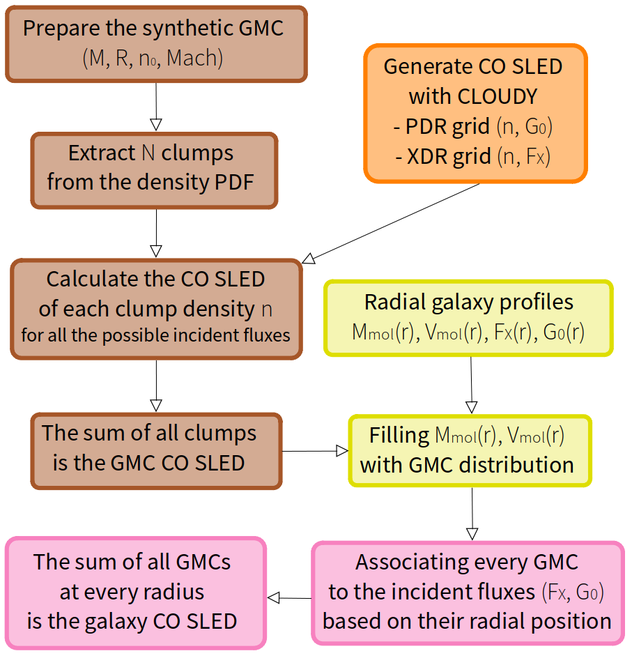
Figure 1: A sketch of the workflow followed in this paper. First, we define a synthetic GMC with four physical variables ($M,R,n_{0},\mathcal{M}$), which define the density distribution of its molecular clumps (as described in Section 2.1). We combine Cloudy results to generate the CO SLED of each clump and of the synthetic GMC (see Section 2.2). Having collected the four radial profiles for a real galaxy ($M_{\text{mol}}(r),V_{\text{mol}}(r),G_{0}(r),F_{\text{X}}(r)$), we filled it with the GMC distribution described in Equation (4), we associate every GMC with the corresponding incident fluxes, and eventually we have the CO SLED of the studied galaxy.

2 Model outline

We build a physically motivated model that decribes the interaction of the radiation from AGN and star formation with the molecular gas in galaxies. This model takes the Vallini et al. (2017, 2018); Vallini et al. (2019) works - focused on the far-infrared (FIR) and molecular line emission from GMCs in high-$z$ galaxies - as starting point. In those works, single GMCs were modelled as collections of clumps in a log-normal density distribution, their CO SLEDs were computed with radiative transfer calculations, and a galaxy was filled with a uniform distribution of identical GMCs. The aim of the present work is to extend such analysis, including different GMCs in single galaxies (following a mass distribution), and illuminating them with a differential radiative flux (following observed radial profiles).

Figure 1 shows a sketch that summarizes its modular structure, which from the sub-pc scales of clumps within GMCs (see Sec. 2.1) progressively zooms-out to the kpc scales of the gas distribution within galaxies (see Sec. 2.3). More precisely, Section 2.1 deals with the analytical description of the internal structure and mass distribution of GMCs, Section 2.2 outlines the RT modelling implemented to compute the CO emission, whereas in Sec. 2.3 we present our assumptions concerning the molecular gas distribution on kpc-scales and the resulting total CO emission from galaxies.

2.1 GMC internal structure and mass distribution

We characterize GMCs with four physical parameters: the total mass ($M$), the GMC radius ($R$), the mean density ($\rho_{0}$) and the Mach number ($\mathcal{M}$). The density structure of GMCs (see e.g. Hennebelle & Falgarone, 2012) is well described by a log-normal distribution (Vazquez-Semadeni, 1994; Padoan & Nordlund, 2011; Federrath et al., 2011; Vallini et al., 2017). The volume-weighted probability distribution function (PDF) of gas density $\rho$, in a supersonically turbulent, isothermal cloud of mean density $\rho_{0}$, is

$$p_{s}\,ds=\frac{1}{\sqrt{(2\pi\sigma_{s}^{2})}}\exp\left[-\frac{1}{2}\left(\frac{s-s_{0}}{\sigma_{s}}\right)^{2}\right]\,ds\;\;,$$ (1)

where $s=\ln(\rho/\rho_{0})$ is the logarithmic density, with mean value $s_{0}=-\sigma_{s}^{2}/2$. The standard deviation of the distribution, $\sigma_{s}$, depends on $\mathcal{M}$ and on the $b$ factor, which parametrizes the kinetic energy injection mechanism (often referred to as forcing) driving the turbulence (Molina et al., 2012):

$$\sigma_{s}^{2}=\ln\left(1+b^{2}\mathcal{M}^{2}\right)\;\;.$$ (2)

We assume $b=0.3$, which is the value for purely solenoidal forcing (Federrath et al., 2008; Molina et al., 2012).

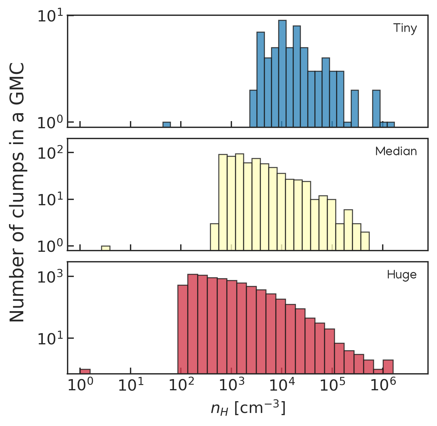
Figure 2: Histograms of clumps density distributions within the three GMCs listed in Table 1. The shapes are set from Equation 1, and mainly depend on each GMC mean number density $n_{0}$.

Name	M [M⊙]	R [pc]	n0 [cm-3]	N${}_{\mbox{clumps}}$
Tiny	$1.3\times 10^{3}$	$1.5$	$2755.6$	$69$
Median	$3.2\times 10^{4}$	$7.7$	$549.8$	$674$
Huge	$7.9\times 10^{5}$	$38.6$	$109.7$	$7644$

Table 1: Main properties of the smallest, median and largest GMCs in the mass distribution described in Section 2.1. The columns are the mass, radius, mean number density and number of extracted clumps.

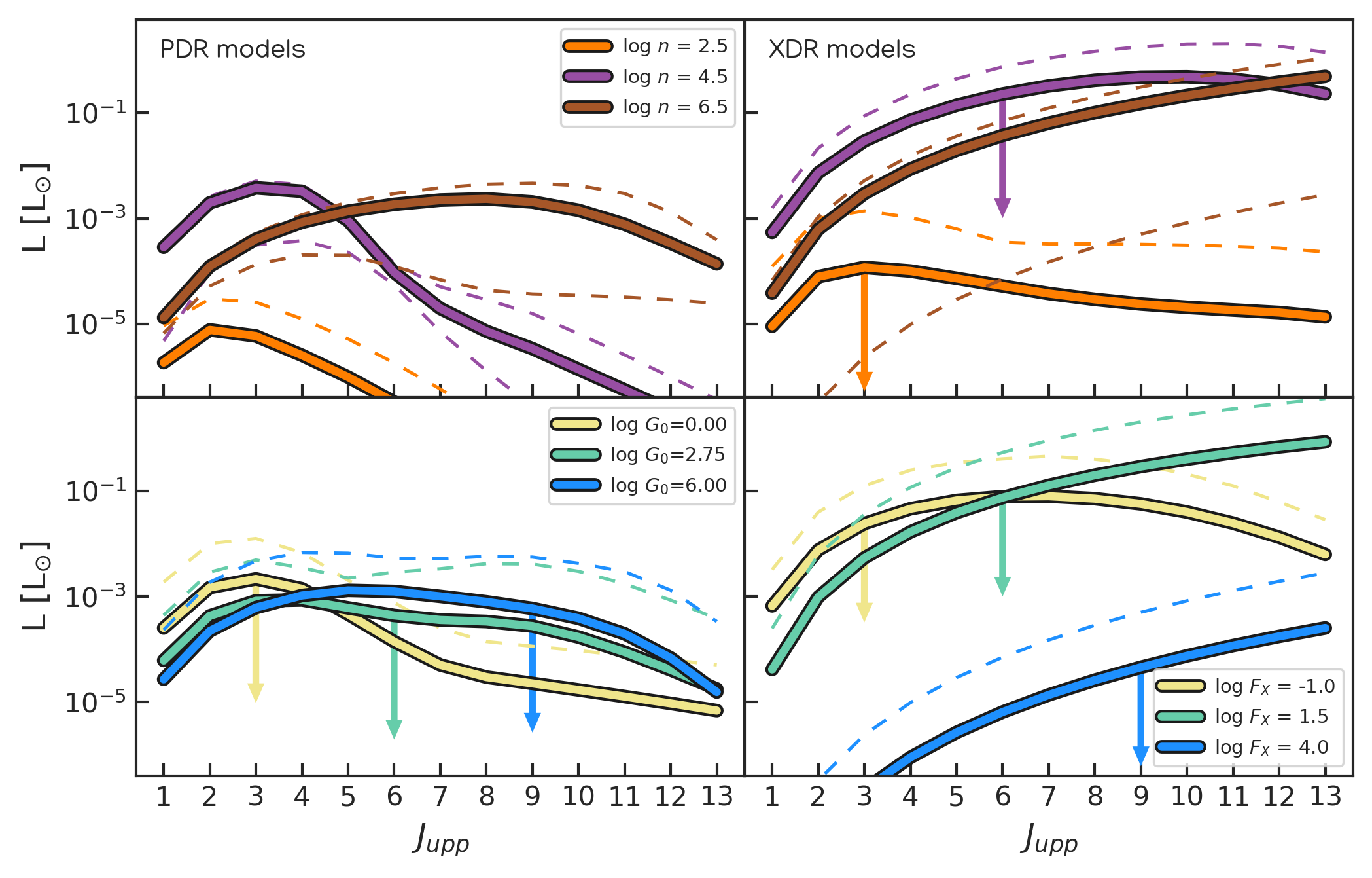
Figure 3: Synthetic CO SLEDs from CO($1-0$) to CO($13-12$) for spherical molecular clumps of radius $R=R_{J}$ (Equation 3). The clump fluxes have been converted to solar units. Left and right panels are PDR and XDR models, respectively. In the upper panels the orange, purple, and brown lines represent the mean CO SLED for $\log n=2.5,\,3.5,\,4.5\,\rm{cm^{-3}}$, respectively, with the incident flux ($G_{0}$ for PDRs, $F_{\text{X}}$ for XDRs) left free to vary over the ranges $10^{0}-10^{6}$ and $10^{-1}-10^{4}$ erg s^-1 cm^-2, respectively. In the lower panels the yellow, green, and blue lines represent the median CO SLED for $\log G_{0}=0.0,\,2.75,\,6.0$ (bottom-left panel) and for $\log F_{\text{X}}=-1.0,\,1.5,\,4.0\,\rm{ergs^{-1}cm^{-2}}$ (bottom-right panel), respectively, while the volume density is left free to vary over the range $10^{0}-10^{6.5}\rm{cm^{-3}}$. In all panels the solid lines represent the mean CO SLED, while the dashed lines with the same colors show the minimum and maximum CO SLEDs at the given density or incident flux. If the minimum luminosity of a given SLED is out of the plot, then the median curve is plotted with a downward arrow to highlight the presence of very low luminosities.

We define a GMC as a spherical collection of clumps, whose densities are distributed following the PDF in Equation (1). Accounting for the presence of clumps within the GMCs is one of the fundamental features of this work, as dense clumps emit the bulk of the CO luminosity ($n_{\text{crit}}>10^{4}$ cm^-3 for $J\geq 2$, Carilli & Walter, 2013). We then randomly extract clumps with $\rho\geq\rho_{0}$ from the PDF and for each of them we calculate its Jeans mass, $M_{J}=(4\pi/3)R_{J}^{3}\mu m_{p}n$, and the Jeans radius:

$$R_{J}(n)=\sqrt{\frac{\pi c_{s}^{2}}{G\rho}}\;\;.$$ (3)

Here $c_{s}=\sqrt{\gamma k_{B}T/(\mu m_{p})}$ is the sound speed, that depends, after we set the adiabatic index to $\gamma=5/3$ and the mean molecular weight to $\mu=1.22$, only on the gas temperature $T$ and the clump number density $n$. We assume a fixed temperature of $T=10$ K for all our clumps, which is the typical value for dense clumps in molecular clouds (Spitzer, 1978; Hughes et al., 2016; Elia et al., 2021). We proceed with the clumps extraction until we fill the entire GMC mass (with a $10\%$ tolerance). Following Vallini et al. (2017), we distribute the leftover mass through the whole GMC, accounting for what we define intraclump medium (ICM).

We consider 15 different GMC models, with masses in the range $M=10^{3}-10^{6}\,\rm M_{\odot}$ (0.2 dex steps), and a fixed surface density $\Sigma=170\,\rm M_{\odot}\,pc^{-2}$ (McKee & Ostriker, 2007). This translates into GMCs radii in the range $R=1-40\,\rm pc$, and mean number densities, $n_{0}=3M/(\mu m_{p}4\pi R^{3})$, in the range $n_{0}=10^{2}-3\times 10^{3}\,\rm cm^{-3}$. The Mach number is set to $\mathcal{M}=10$ for all the GMCs in this work (Krumholz & McKee, 2005). In Figure 2 we plot the distribution in density of the clumps within the three GMCs listed in Table 1: different GMCs (shown with different colors) have a different peak in the clumps density distribution, since they have a different mean density $n_{0}$. The ICM appears, in Figure 2, in single clumps at low-end densities.

The observed GMC mass distribution in galaxies is well approximated by a power-law (see Chevance et al., 2023, for a recent review). In particular, we follow Roman-Duval et al. (2010) and Dutkowska & Kristensen (2022) and we set the mass distribution as follows:

$$\frac{dN}{dM}\propto M^{-1.64}.$$ (4)

Equation (4) has been derived by fitting the observed GMC mass distribution in the Milky Way with a power-law, albeit only in the mass range $M=10^{5}-10^{6}\,\rm M_{\odot}$ due to observational limits that make it hard to sample the distribution towards the low-mass end (Roman-Duval et al., 2010). Dutkowska & Kristensen (2022) extrapolate the relation down to $M=10^{4}\,\rm M_{\odot}$, but in this work we extrapolate Equation (4) down to $M=10^{3}\rm\,M_{\odot}$, because we expect the majority of GMCs in galaxies to be small and with low masses (e.g. Fukui & Kawamura, 2010; Colombo et al., 2014; Rosolowsky et al., 2021).

We verified that the choice of different power-law exponents for Equation (4), namely 1.39, 1.89 and 2.5, corresponding to the lowest and highest values in Roman-Duval et al. (2010) and the highest value from Chevance et al. (2023) does not greatly affect our results. In Table 1, we list the two extremes in mass, labelled as "Tiny" and "Huge", respectively, and the "Median" GMCs, extracted from the distribution.

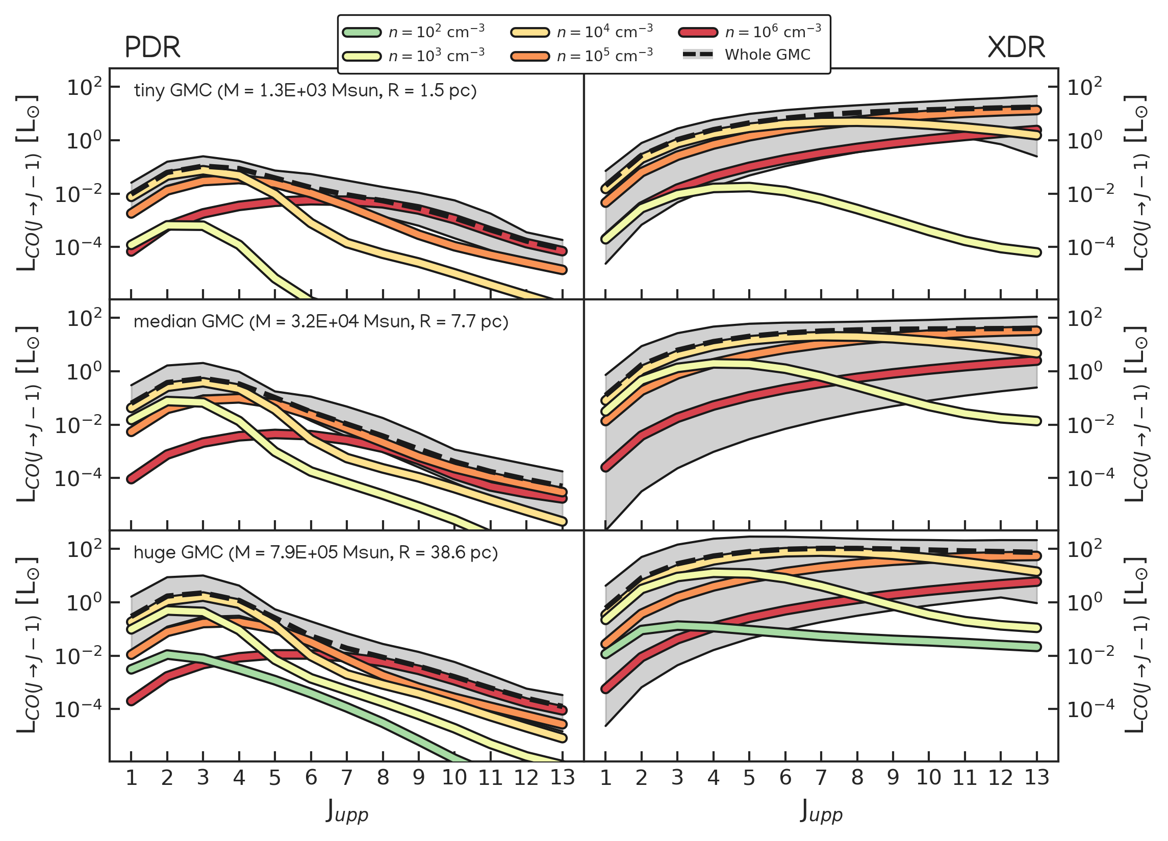
Figure 4: CO SLED of the three GMCs listed in Table 1. The dashed black lines represent the CO SLED of the tiny (upper panels), median (middle panels), huge (lower panels) GMC models, while the grey shaded area highlights the variation in the GMC CO SLED produced by changing the incident flux. Left panels are for PDR models (i.e. the incident flux range is $10^{0}\leq G_{0}\leq 10^{6}$), right panels are for XDR models (i.e. the incident flux range is $10^{-1}\leq F_{\text{X}}/(\rm{erg\,s^{-1}\,cm^{-2}})\leq 10^{4}$). The colored lines highlight the contribution of the clumps within each GMC, as a function of their density $n$.

2.2 Radiative transfer modelling

We use Cloudy (version 17.02, Ferland et al., 2017) to model the CO line emission from a 1-D gas slab with constant density $n$ and irradiated by a stellar or AGN incident flux. In what follows we label a Cloudy run as "PDR-model" if the incident far-ultraviolet (FUV) photons flux is produced by a stellar population. As it is a standard in PDR studies (Wolfire et al., 2022) the FUV flux ($G_{0}$) is parametrized in terms of the Habing field $1.6\times 10^{-3}\,\rm erg\,s^{-1}\,cm^{-2}$ (Habing, 1968), which equates to $G_{0}=1$. Conversely, we label a run as "XDR-model" if the incident flux $F_{\text{X}}$ (in the $1-100\rm\,keV$ range) comes from an AGN.

For PDR models we adopt the Spectral Energy Distribution (SED) of the incident radiation from the stellar population synthesis code Starburst99 (Leitherer et al., 1999), assuming a continuous star formation model with age $t=10\,\rm Myr$ and solar metallicity, and $\log(G_{0})=0-6$. In the XDR models, we use $\log[F_{\text{X}}/(\text{erg s}^{-1}\text{ cm}^{-2})]=-1-4$, and the SED is set with the Cloudy command table xdr, that generates a truncated AGN X-ray SED, $f_{\nu}\propto h\nu^{-0.7}$, in the 1–100 keV range (see Maloney et al., 1996, for details).

The second free parameter in the PDR and XDR models is the gas density $n$. To cover the density range of clumps and ICM in GMCs (see Section 2.1), we consider a grid of Cloudy runs spanning $\log(n/\text{cm}^{-3})=0-6.5$. The ranges of $n$, $G_{0}$ and $F_{\text{X}}$ have logarithmic steps of 0.25 dex. All our Cloudy runs assume solar metallicity for the gas, and elemental abundances from Grevesse et al. (2010). Moreover, we account for the Cosmic Microwave Background ($T_{\rm CMB}=2.7$ K), the Milky Way cosmic ray ionization rate, $\zeta=2\times 10^{-16}$ s^-1 (Indriolo et al., 2007), and we set the turbulence velocity $v=1.5\rm\,km\,s^{-1}$ (see Pensabene et al., 2021).

Cloudy solves the RT through the gas slab by dividing it into a large number of thin layers. Starting at the illuminated face of the slab, it computes the cumulative emergent flux at every layer. While in this work we are interested in the CO lines from CO($1-0$) to CO($13-12$), Cloudy also computes other molecular and atomic lines (e.g. HCN, HCO⁺, [CII]) that we store in our database. We compute the emergent line emission up to a total gas column density of $\log(N_{\text{H}}/\rm cm^{-2})=24.5$: this choice allows us to fully sample the molecular part of the irradiated gas clouds, typically located at $N_{\text{H}}>2\times 10^{22}$ cm^-2 (McKee & Ostriker, 2007). The CO emission from a GMC is obtained by interpolating the Cloudy outputs at the density $n_{i}$ and radius $R_{i}$ for each $i$-th clump and then summing up all the clumps luminosities.

2.2.1 The CO SLED of single clumps and GMCs

In what follows, we first discuss the resulting CO SLED from clumps of different densities within a given GMC, noting that the luminosity of each $i$-th clump is $L=4\pi R_{i}^{2}F_{CO}(R_{i})$, where $F_{CO}(R_{i})$ is the flux computed by Cloudy. This is shown in Figure 3.

As shown in the upper panel of Figure 3 the CO SLEDs for XDR clump models are overall brighter at a given gas density, with respect to the CO SLEDs of PDR clump models. Leaving the incident flux free to vary (upper panels of Figure 3) has a limited effect in the CO cooling energy output of PDR models (top-left panel). Varying the incident flux seems more important in XDR models (top-right panel), since the derived CO SLED luminosities can decrease by more than four orders of magnitudes (as pointed by the downward arrows in the top-right panel of Figure 3).

Leaving the density free to vary while fixing the incident flux, however, could make the CO SLED luminosity range over several orders of magnitude for any possible value of incident flux, both for PDR and XDR models (bottom panels of Figure 3). The very low-luminosity SLEDs correspond to the lowest densities computed ($\log n/{\rm cm^{-3}}=0$). It is interesting to note that the highest $F_{\text{X}}$ values, which correspond to clumps closer to the AGN, return very faint CO SLEDs: this is because high X-ray photon fluxes lead to the CO dissociation (see Wolfire et al., 2022, for a recent review of XDR processes).

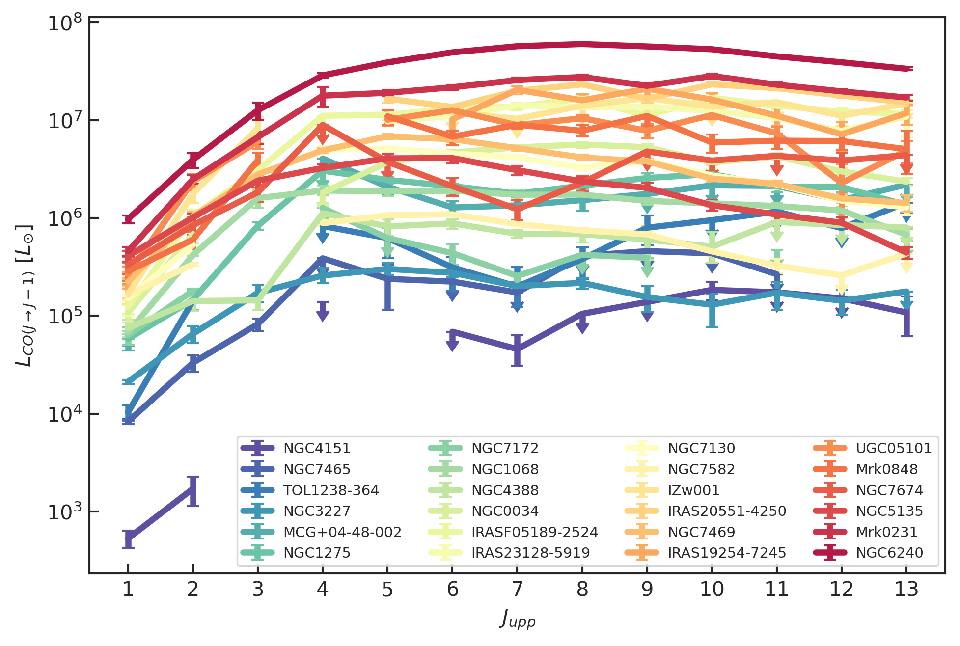
Figure 5: Observed CO SLED of our AGN sample, composed of 24 galaxies. The order of the objects depends on their molecular mass within a radius of $2r_{\text{CO}}$ (blue is low, red is high, with the range being [$5\times 10^{7}-9\times 10^{10}$] M_⊙ when calculated with a Milky-Way $\alpha_{\text{CO}}$). Downward arrows are upper limits.

As detailed in Section 2.1, for a given modelled cloud we have a list of extracted clumps. Once the contribution from the various clumps in the GMC is accounted for, by summing up their CO luminosity, the global CO SLED of a GMC depends on the incident flux only. In Figure 4, we show the CO SLED for the three GMCs listed in Table 1. The variation in the GMC CO SLED introduced by spanning the whole $G_{0}$ and $F_{\text{X}}$ ranges is highlighted by a grey shaded area. We note that varying $G_{0}$ has a limited effect on the predicted CO SLEDs (left panels in Figure 4), as opposed to varying $F_{\text{X}}$ (right panels).

In Figure 4 we plot the contribution of clumps of different densities to the global GMC CO SLED. PDR models (left panels of Figure 4) are dominated by clumps with density $n=10^{4},10^{5},10^{6}\,\rm cm^{-3}$ in the low ($J\leq 4$), medium ($5\leq J\leq 7$) and high-$J$ ($J\geq 8$) transitions, respectively. In the XDR case (right panels of Figure 4), instead, the very high-density clumps ($n\sim 10^{6}$ cm^-3) never dominate the CO SLED: their contribution is always at least one order of magnitude lower than clumps with $n=10^{4}-10^{5}\,\rm cm^{-3}$. However, as can be noticed in Figure 3, the very high-density clumps can sustain a high XDR emission only when a large incident flux ($F_{\text{X}}\sim 10^{4}$ erg s^-1 cm^-2) is present. This is because at high volume and, thus, column densities ($N_{\text{H}}=nR_{J}\propto n^{1/2}$), the molecular gas is efficiently shielded from external radiation, so that only a large incident flux can penetrate the gas. The same argument applies to PDRs.

2.3 Galaxy radial profiles

In this Section we describe how we distribute the GMCs throughout the galaxy volume, and how we associate to each GMC an incident flux ($G_{0}$ or $F_{\text{X}}$) depending on the position within the galaxy. To do so, we need the radial profiles of the molecular mass $M_{\text{mol}}(r)$, the molecular volume $V_{\text{mol}}(r)$, the FUV flux $G_{0}(r)$, and the X-ray flux $F_{\text{X}}(r)$. Spatially resolved observations of nearby galaxies have shown that low-$J$ CO emission is well described by an exponential profile along the galactocentric radius $r$ (Boselli et al., 2014; Casasola et al., 2017, 2020), with scale factor $r_{\text{CO}}=0.17r_{25}$, where $r_{25}$ is the radius of the galaxy at the isophotal level 25 mag arcsec^-2 in the B-band. The CO($1-0$) emission can be converted into the molecular mass by adopting a CO-to-H₂ conversion factor $\alpha_{\text{CO}}$ (e.g. Bolatto et al., 2013, for a review). We adopt the Milky Way value of $\alpha_{\text{CO}}=4.3$ M_⊙ (K km s^-1 pc²)^-1 (which includes the helium contribution) as our initial fiducial value, but we will discuss the effect of relaxing this assumption in Section 5.1. We thus obtain the following cumulative molecular mass radial profile:

$$M_{\text{mol}}(r)=2.08\times 10^{4}\,\alpha_{\text{CO}}\,L_{\text{CO,tot}}\,[1-e^{-r/r_{\text{CO}}}(r/r_{\text{CO}}+1)]$$ (5)

where $L_{\text{CO,tot}}$ is the CO($1-0$) luminosity of the whole galaxy in L_⊙, $M_{\text{mol}}$ is in M_⊙. This molecular gas mass is also confined within a volume radial profile $V(r)$. We approximate the galaxy as a disc, with half-height $z_{\text{CO}}=0.01r_{25}$ (Boselli et al., 2014; Casasola et al., 2020), in its external part, while in its inner part ($r<1.5\,z_{\text{CO}}$) we use the equation for a sphere to model a bulge:

$$V_{\text{mol}}(r)=\begin{cases}(4/3)\pi r^{3}&\text{for $r\leq 1.5\,z_{\text{CO}}$}\\ 2\pi z_{\text{CO}}r^{2}&\text{for $r\geq 1.5\,z_{\text{CO}}$}\end{cases}$$ (6)

The profile $V(r)$ changes at $r=1.5z_{\text{CO}}$ to ensure a smooth transition between the spherical and the disc-like regions. Equations (5) $-$ (6) imply that the molecular gas volume density $\rho_{\text{mol}}(r)$ increases towards small radii. The gas surface density $\Sigma(r)$ is instead roughly constant in the central part (i.e. at $r\lesssim r_{\text{CO}}$), and decreases exponentially as $\Sigma_{\text{mol}}(r)=\Sigma_{\text{mol}}(0)e^{-r/r_{\text{CO}}}$.

In our model the molecular gas – distributed according to Equations (5) $-$ (6) – is irradiated by a FUV or X-ray flux that depend on the galactocentric radius. Following E22, we model $G_{0}(r)$ with a Sersic function (Sérsic, 1963):

$$G_{0}(r)=G_{0}(r_{e})\exp\left\{-b_{n}\left[\left(\frac{r}{r_{e}}\right)^{1/n}-1\right]\right\}$$ (7)

which is characterized by three parameters: the effective radius $r_{e}$, the shape parameter $n$ and the normalization $G_{0}(r_{e})$. We assume a minimum $G_{0}=1$ at every radius, which is equal to the Milky Way interstellar radiation field (ISRF).

The X-ray profile, $F_{\text{X}}(r)$, is derived from the intrinsic X-ray luminosity $L_{\text{X}}$, in the $1-100\,\rm keV$ range. Given the importance of the attenuation of the X-ray flux due to obscuring gas, usually measured in terms of gas column density $N_{\text{H}}(r)$, we use the following formula (Maloney et al., 1996; Galliano et al., 2003):

$$F_{\text{X}}(r)=\frac{L_{\text{X}}}{4\pi r^{2}}N_{22}(r)^{-0.9}$$ (8)

where $N_{22}(r)=N_{\text{H}}(r)/10^{22}\rm\,cm^{-2}$.

From the derived radial profiles of the molecular mass and volume, we can easily compute the column density radial profile as

$$N_{\text{H}}(r)=\int_{0}^{r}n_{\text{H}}(x)\,dx=\int\frac{M_{\text{mol}}(x)}{\mu m_{p}V_{\text{mol}}(x)}\,dx\;\;\;.$$ (9)

Whenever the gas column density $N_{\text{H}}(r)<10^{22}\rm\,cm^{-2}$, due to the marginal impact on the X-rays attenuation (e.g. Hickox & Alexander, 2018), we use the classical definition $F_{\text{X}}(r)=L_{\text{X}}/(4\pi r^{2})$. We term this "Baseline model", as it is also possible to fit the average $N_{\text{H}}$ value from the observed CO SLEDs (see Section 4). We will discuss in detail the effect of $N_{\text{H}}(r)$ in Section 5.2.

3 The dataset

In E22, we gathered a wealth of observational data for a sample of 35 local ($z\leq 0.15$) AGN-host galaxies. For each source we collected: CO line luminosities from CO($1-0$) to CO($13-12$), mostly coming from Herschel observations; the optical radius $r_{25}$ (from the HyperLeda database); the total IR luminosity $L_{\text{IR}}$ ($8-1000$ $\mu$m), mostly from IRAS observations; the intrinsic X-ray luminosity $L_{\text{X}}$ ($2-10\,\rm keV$) and the obscuring column density of the X-ray photons, $N_{\text{H, X-ray}}$, from a variety of X-ray observatories; and the FIR flux (observed by Herschel) from which we derived the FUV field radial profile, $G_{0}(r)$ (i.e. the three parameters of Equation 7: $G_{0}(r_{e})$, $r_{e}$, and $n$). Any change in the data with respect to E22 is reported in Appendix A.

First of all, we select a sub-sample of the 35 galaxies analyzed in E22. We adopt the following selection criteria: (i) the availability of the CO($1-0$) detection, necessary for the derivation of the molecular gas mass of a galaxy; (ii) the availability of both incident flux radial profiles, i.e. $G_{0}(r)$ and $F_{\text{X}}(r)$; (iii) an apparent optical radius $r_{25}\leq 250^{\prime\prime}$, since larger objects would have a $r_{\text{CO}}$ larger than the CO beams; (iv) at least three CO detections (i.e. without counting the upper limits) between CO($1-0$) and CO($13-12$), to ensure we have enough data points to make a meaningful comparison with the model output. These selection criteria reduce our sample to 24 active galaxies. We list, in Table 2, the $r_{\text{CO}}$, the median $G_{0}(r)$, the $L_{\text{X}}$ and the $N_{\text{H, X-ray}}$ of each galaxy in the sample.

The parent sample was selected considering the availability of Herschel data, and being their intrinsic X-ray luminosity $L_{\text{X}}\geq 10^{42}$ erg s^-1 in the $2-10$ keV range. The sample of 24 objects considered in this work is composed by nearby ($z\leq 0.062$) moderately powerful ($L_{\text{X}}\leq 10^{44}$ erg s^-1) AGN-host galaxies, but at the same time they display a wide variety of physical properties. Four galaxies of our sample (IRAS 19254$-$7245, IRAS 23128$-$5919, Mrk 848, and NGC 6240) are clear mergers, while other six (IRAS F05189$-$2524, IRAS 20551$-$4250, Mrk 231, NGC 34, NGC 1275, and UGC 5101) show some signs of interaction as tidal tails. The rest of the sample has a spiral-like morphology. Half of the galaxies (12/24) are luminous infrared galaxies (LIRGs: $10^{11}\leq L_{\text{IR}}<10^{12}$ L_⊙), while 5 are ultra-LIRGs (ULIRGs: $L_{\text{IR}}\geq 10^{12}$ L_⊙). Almost all of the galaxies (22/24) have their nuclear activity classified as Seyfert, with the exceptions of Mrk 848 and IRAS 20551$-$4250 which are classified as low-ionization nuclear emission-line regions (LINERs). NGC 1275 (also known as 3C 84, Perseus A) is the only radio-galaxy of our sample, and it is also the central dominant galaxy in the Perseus Cluster. Two of the furthest galaxies (Mrk 231 and I Zw 1) are also commonly classified as quasi-stellar objects (QSOs). We refer to E22 for further details on the galaxy sample and data collection. The CO SLEDs of all the objects in our sample are shown in Figure 5.

Table 2: Properties and results on the sample of 24 AGN.

	$r_{\text{CO}}$	$\log M_{\text{mol}}$	$\log G_{0}$	$\log L_{\text{X}}$	$\log N_{\text{H,X}}$	$f_{\text{PDR}}^{\text{(1-0)}}$	$f_{\text{XDR}}^{\text{(1-0)}}$	$f_{\text{PDR}}^{\text{(4-3)}}$	$f_{\text{XDR}}^{\text{(4-3)}}$	$\alpha_{\text{CO}}$	$\log N_{\text{H}}$
Name	(kpc)	(M⊙)		(erg s-1)	(cm-2)						(cm-2)
I Zw 1	2.78	10.36	1.64	43.6	$-$	0.76	0.20	0.24	0.80	$6.6^{+1.7}_{-1.7}$	$23.50^{+0.37}_{-0.28}$
IRAS F05189$-$2524	2.15	9.74	3.83	43.2	22.86	0.17	0.02	0.83	0.98	$2.1^{+0.4}_{-0.2}$	$22.09^{+0.12}_{-0.04}$
IRAS 19254$-$7245	3.83	10.55	3.94	42.8	23.58	0.57	0.11	0.43	0.89	$7.3^{+1.5}_{-0.9}$	$22.11^{+0.10}_{-0.05}$
IRAS 20551$-$4250	2.92	10.46	4.22	42.3	23.69	0.64	0.14	0.36	0.86	$7.2^{+0.9}_{-0.6}$	$22.04^{+0.04}_{-0.02}$
IRAS 23128$-$5919	4.18	10.15	3.71	43.2	$-$	0.46	0.07	0.54	0.93	$5.5^{+1.0}_{-0.4}$	$22.08^{+0.10}_{-0.03}$
MCG +04$-$48$-$002	1.45	9.85	2.54	43.1	23.86	0.81	0.27	0.19	0.73	$7.3^{+1.3}_{-1.3}$	$23.96^{+0.10}_{-0.12}$
Mrk 231	5.99	10.95	4.77	42.5	22.85	0.86	0.34	0.14	0.66	$9.4^{+0.5}_{-0.5}$	$22.02^{+0.01}_{-0.02}$
Mrk 848	2.62	10.26	3.72	42.3	23.93	0.66	0.15	0.34	0.85	$3.1^{+0.4}_{-0.3}$	$22.05^{+0.04}_{-0.03}$
NGC 34	2.33	10.20	2.93	42.1	23.72	0.77	0.21	0.23	0.79	$7.1^{+0.5}_{-0.8}$	$22.07^{+0.03}_{-0.04}$
NGC 1068	2.46	9.88	3.69	42.4	24.70	0.80	0.24	0.20	0.76	$5.4^{+0.9}_{-0.5}$	$22.40^{+0.10}_{-0.04}$
NGC 1275	3.89	8.78	3.60	44.0	21.68	0.25	0.02	0.75	0.98	$0.5^{+0.1}_{-0.0}$	$22.11^{+0.17}_{-0.08}$
NGC 3227	1.62	8.94	3.00	42.1	20.95	0.74	0.16	0.26	0.84	$2.0^{+0.2}_{-0.3}$	$22.53^{+0.07}_{-0.09}$
NGC 4151	1.01	7.30	2.28	42.3	22.71	0.66	0.11	0.34	0.89	$1.8^{+0.7}_{-0.5}$	$22.66^{+1.02}_{-0.47}$
NGC 4388	4.74	9.16	2.90	42.6	23.50	0.87	0.30	0.13	0.70	$0.9^{+0.1}_{-0.1}$	$22.02^{+0.01}_{-0.02}$
NGC 5135	3.42	10.27	3.11	42.0	24.47	0.86	0.32	0.14	0.68	$2.2^{+0.2}_{-0.2}$	$22.03^{+0.06}_{-0.03}$
NGC 6240	5.51	10.60	4.10	43.6	24.20	0.54	0.07	0.46	0.93	$2.0^{+0.1}_{-0.1}$	$22.05^{+0.02}_{-0.02}$
NGC 7130	2.60	10.05	3.68	42.3	24.10	0.76	0.19	0.24	0.81	$3.6^{+0.5}_{-0.5}$	$22.08^{+0.08}_{-0.05}$
NGC 7172	2.28	9.75	2.67	42.8	22.91	$-$	$-$	$-$	$-$	$-$	$-$
NGC 7465	0.74	8.91	2.48	42.0	21.46	0.96	0.64	0.04	0.36	$4.7^{+0.7}_{-0.7}$	$23.94^{+0.65}_{-0.48}$
NGC 7469	2.34	10.39	3.30	43.2	20.53	0.83	0.29	0.17	0.71	$5.3^{+0.5}_{-0.7}$	$23.54^{+0.05}_{-0.09}$
NGC 7582	3.82	9.58	3.25	42.5	24.20	0.46	0.06	0.54	0.94	$1.1^{+0.2}_{-0.1}$	$22.29^{+0.10}_{-0.07}$
NGC 7674	3.32	10.27	4.06	43.6	$-$	0.94	0.54	0.06	0.46	$2.7^{+0.4}_{-0.4}$	$24.08^{+0.11}_{-0.12}$
TOL 1238-364	1.44	9.14	3.45	43.4	24.95	0.83	0.28	0.17	0.72	$6.5^{+1.2}_{-1.1}$	$24.09^{+0.14}_{-0.14}$
UGC 5101	4.78	10.58	4.36	43.1	24.08	0.78	0.22	0.22	0.78	$6.9^{+1.3}_{-1.2}$	$22.51^{+0.10}_{-0.11}$

• Notes. The molecular masses $M_{\text{mol}}$ are calculated within a $2\,r_{\text{CO}}$ radius and by using the best-fit $\alpha_{\text{CO}}$ (except for NGC 7172, for which we used $\alpha_{\text{CO}}=4.3$). $G_{0}$ is the median value of the $G_{0}(r)$ profile. $N_{\text{H,X}}$ is the column density derived from the X-ray SED. The best-fit $f_{\text{PDR}}^{\text{(1-0)}}$, $f_{\text{XDR}}^{\text{(1-0)}}$, $f_{\text{PDR}}^{\text{(4-3)}}$, and $f_{\text{XDR}}^{\text{(4-3)}}$ are the fractions to the total CO($1-0$) and CO($4-3$) luminosities, respectively, due to PDR and XDR emission, respectively. Best-fit $\alpha_{\text{CO}}$ is in units of M_⊙ (K km s^-1 pc²)^-1. For both $\alpha_{\text{CO}}$ and $\log N_{\text{H}}$, we report the median values of the marginalized posterior distributions, with $1\sigma$ width as errors.

4 Results

The model takes into account the radial profiles defined in Equations (5) $-$ (9) to spatially distribute the 15 GMCs described in Section 2.1 in a real galaxy. The profiles for all the galaxies in the E22 sample are presented in Figure 13. We divide these profiles into logarithmically-spaced radial bins. Based on some tests, we adopt a 0.05 dex bin size, starting from $r_{\text{min}}=10^{-3}$ kpc, and up to $r_{\text{max}}=2r_{\text{CO}}$. First, since for every bin we know the molecular mass and the molecular volume, we extract random GMCs from the distribution (Equation 4), until we fill up the entire mass and/or volume of the bin. Then, we associate each GMC, in each radial bin, with the matching incident fluxes $G_{0}(r)$, $F_{\text{X}}(r)$, and finally produce the expected CO SLED of each galaxy.

4.1 The different models

The molecular mass of a galaxy is highly dependent on the choice of the CO-to-H₂ conversion factor $\alpha_{\text{CO}}$, while the X-ray flux can be strongly attenuated by gas clouds between the AGN and the GMCs which we parametrize in terms of a hydrogen column density profile $N_{\text{H}}(r)$.

The model discussed in Section 2 assumes a default Milky-Way value of $\alpha_{\text{CO}}=4.3$ M_⊙ (K km s^-1 pc²)^-1, and the intrinsic $N_{\text{H}}(r)$ profile from Equation (9). We label this "Baseline model".

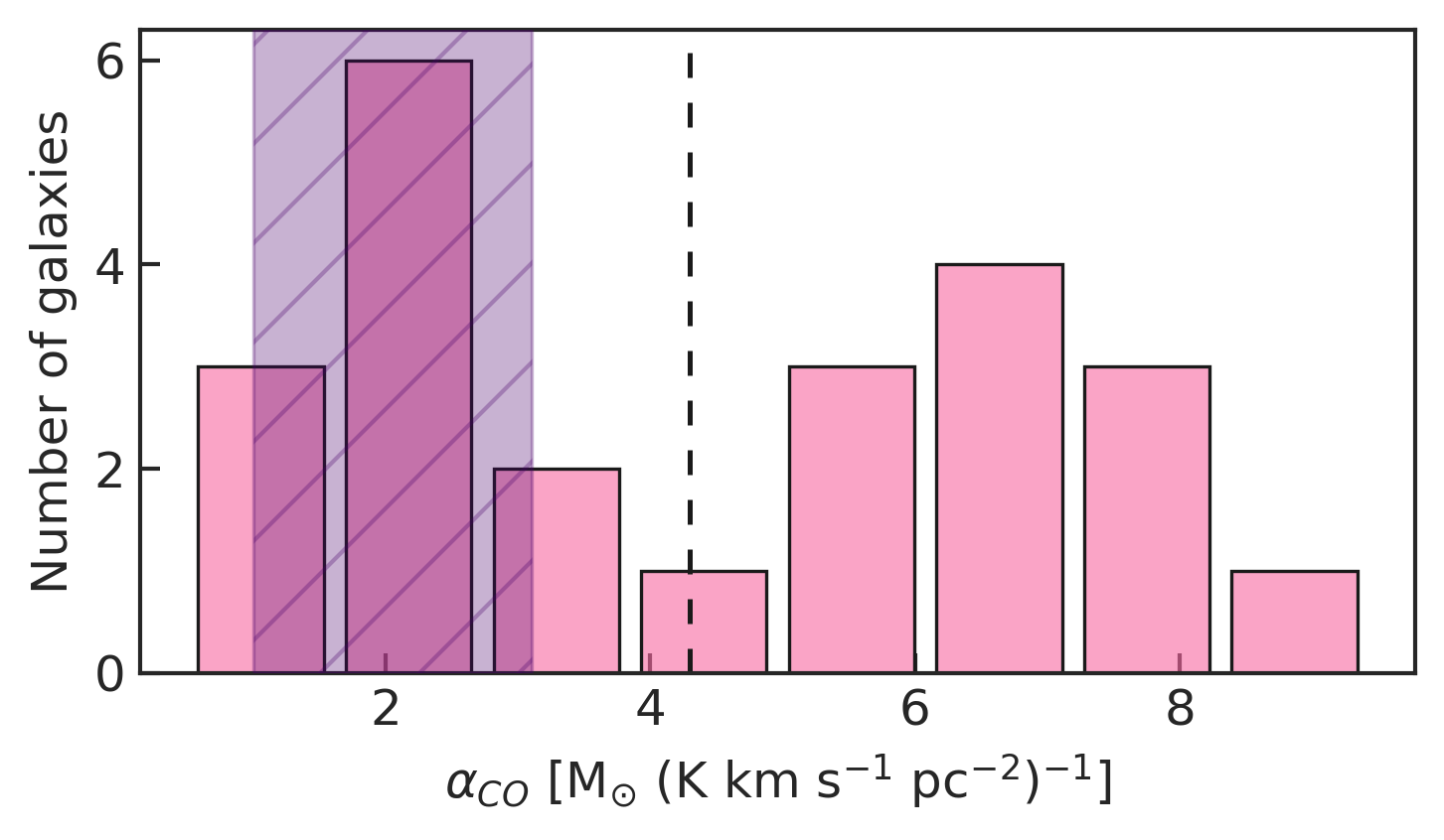
Figure 6: Histogram representing the best-fit CO-to-H₂ conversion factor $\alpha_{\text{CO}}$, selected through the minimization of the $\chi_{\nu}^{2}$, for our sample of 24 galaxies. The dashed line is for the Milky Way value (Bolatto et al., 2013), while the shaded hatched area highlights the values associated to ULIRGs (Pérez-Torres et al., 2021).

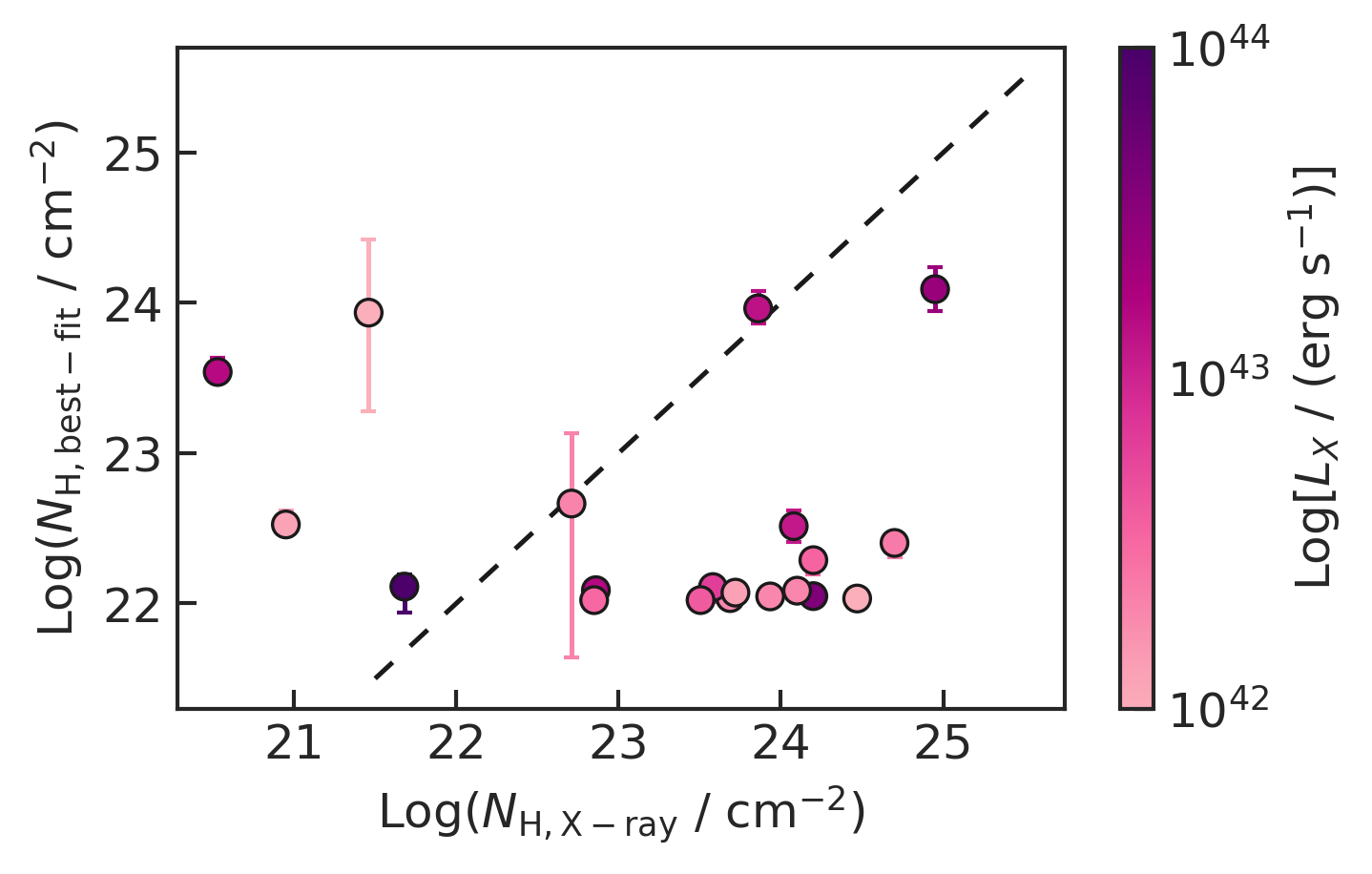
Figure 7: A comparison of the column densities $N_{\text{H}}$ from our fitting procedure (on the $y$-axis) and the $N_{\text{H, X-ray}}$ derived by modelling the absorption of X-rays (on the $x$-axis). The colour of each circle (i.e. of each galaxy) depends on the intrinsic X-ray luminosity $L_{\text{X}}$ ($2-10$ keV). The dashed line is the 1:1 line.

For each galaxy we search also for the "Best-fit model" following the Bayesian Markov chain Monte Carlo (MCMC) method: we use the $\chi^{2}$ likelihood function to fit the observed CO SLED and determine the posterior probability distribution of the model parameters, i.e. $\alpha_{\text{CO}}$ and $N_{\text{H}}$, with uniform prior distributions $\alpha_{\text{CO}}=[0.43,\,43]$ and $N_{\text{H}}=[10^{22}$, $10^{25}$] cm^-2. In this model, $N_{\text{H}}$ has a constant value at every radius, and it acts as an average $N_{\text{H}}$ seen by the GMCs. To run the MCMC algorithm, we use the open-source Python package emcee (Foreman-Mackey et al., 2013), which implements the Goodman and Weare’s Affine Invariant MCMC Ensemble sampler (Goodman & Weare, 2010). In this way we are able to fully characterize any degeneracy between our model parameters, while also providing the 1$\sigma$ spread of the posterior distribution for each of them. To be able to include also upper limits in the likelihood function, we follow the approach described in Sawicki (2012) and Boquien et al. (2019), splitting the $\chi^{2}$ formula in two sums:

$$\chi^{2}=\sum_{j=1}^{13}\left(\frac{f_{j}-m_{j}}{\sigma_{j}}\right)-2\sum_{j=1}^{13}\ln\left\{\frac{1}{2}\left[1+\operatorname{erf}\left(\frac{f_{\text{ul},j}-m_{j}}{\sqrt{2}\sigma_{j}}\right)\right]\right\}$$ (10)

where the first sum contains the detections $f_{j}$ and their errors $\sigma_{j}$ ($j$ covers the first 13 lines of the CO SLED), the second one containing the $3\sigma$ upper limits $f_{\text{ul},j}$ (whereas we used the $1\sigma$ upper limit as the measured error $\sigma_{j}$), and in both sums $m_{j}$ are the model values.

Finally, we produce a third set of synthetic CO SLEDs by keeping the default $\alpha_{\text{CO}}=4.3$ M_⊙ (K km s^-1 pc²)^-1 but using the column density $N_{\text{H, X-ray}}$ derived from the absorption of X-rays along the line of sight (Brightman & Nandra, 2011; Ricci et al., 2017; Marchesi et al., 2019; La Caria et al., 2019, and Salvestrini in prep.). We label these CO SLED predictions "$N_{\text{H, X-ray}}$ model". Also in this case we set $N_{\text{H, X-ray}}$ constant at every radius.

4.2 Best-fit model results

We run emcee with 10 walkers exploring the parameter space for $10^{4}$ chain steps. The chains have been initialized by distributing the walkers around $\alpha_{\text{CO}}=4.3$ M_⊙ (K km s^-1 pc²)^-1 and the median $N_{\text{H}}(r)$ for each galaxy (if larger than $10^{22}$ cm^-2, $10^{22}$ cm^-2 otherwise). For each walker, we first run the algorithm with a burn-in chunk of 5000 steps which we later discard. The procedure gives a mean autocorrelation length $\tau=65$ for both $\alpha_{\text{CO}}$ and $N_{\text{H}}$, and a mean acceptance fraction of 0.59. In the following we report the median values of the marginalized posterior probability distributions for the two parameters, with a 68% confidence interval as errors. The MCMC code did not converge for NGC 7172, due to the dominance of upper limits (7, with only 3 detections): in the subsequent paragraphs and sections, we only consider the remaining 23 galaxies of our sample.

The best-fit procedure returns median values $0.5\leq\alpha_{\text{CO}}<9.5$ M_⊙ (K km s^-1 pc²)^-1, as shown in Figure 6. The median CO-to-H₂ conversion factor for our galaxy sample is $\alpha_{\text{CO}}=4.7^{+2.4}_{-2.8}$, where the lower and upper errors are the $16^{\text{th}}$ and $84^{\text{th}}$ percentiles of the sample distribution, respectively. This value is comparable to that of the Milky Way, and the range agrees well with the available literature (e.g. Bolatto et al., 2013; Leroy et al., 2015; Mashian et al., 2015; Accurso et al., 2017; Seifried et al., 2017; Casasola et al., 2017; Dunne et al., 2022).

The best-fit values of $N_{\text{H}}$ are shown in Figure 7 against $N_{\text{H, X-ray}}$. We find values $10^{22.0}\leq N_{\text{H}}\leq 10^{24.1}$ cm^-2 with a median of $\log(N_{\text{H}}/\rm{cm}^{-2})=22.1^{+1.6}_{-0.1}$. By comparison, the 21/24 galaxies for which we have $N_{\text{H, X-ray}}$ have a median $\log(N_{\text{H, X-ray}}/\rm{cm}^{-2})=23.7^{+0.5}_{-1.8}$.

The maximum fitted obscuration of our sample is in TOL 1238-364 ($N_{\text{H}}=10^{24.1}\text{ cm}^{-2}$), which also has the maximum $N_{\text{H, X-ray}}=10^{25}$ cm^-2. As shown in Figure 7, however, the $N_{\text{H}}$ values, derived from the fit of the CO SLED and from the fit of the X-ray spectrum, do not correlate. This, anyway, does not constitute a critical issue of our modelling, as will be explained in Section 5.2.

We find a degeneracy between the $\alpha_{\text{CO}}$ and $N_{\text{H}}$ sampled values in almost all the galaxies (see e.g. Figure 8 for NGC 3227). This is not unexpected, since it is known that $\alpha_{\text{CO}}$ depends on the optical depth (Bolatto et al., 2013; Teng et al., 2023), which in turn depends on $N_{\text{H}}$. Increasing $\alpha_{\text{CO}}$ in a galaxy means more molecular mass within the same volume, hence $N_{\text{H}}$ has to increase accordingly. The galaxies for which the sampled parameters do not show degeneracy are also among the ones for which our model works worse (e.g. Mrk 231, NGC 4151, NGC 4388, see Appendix C).

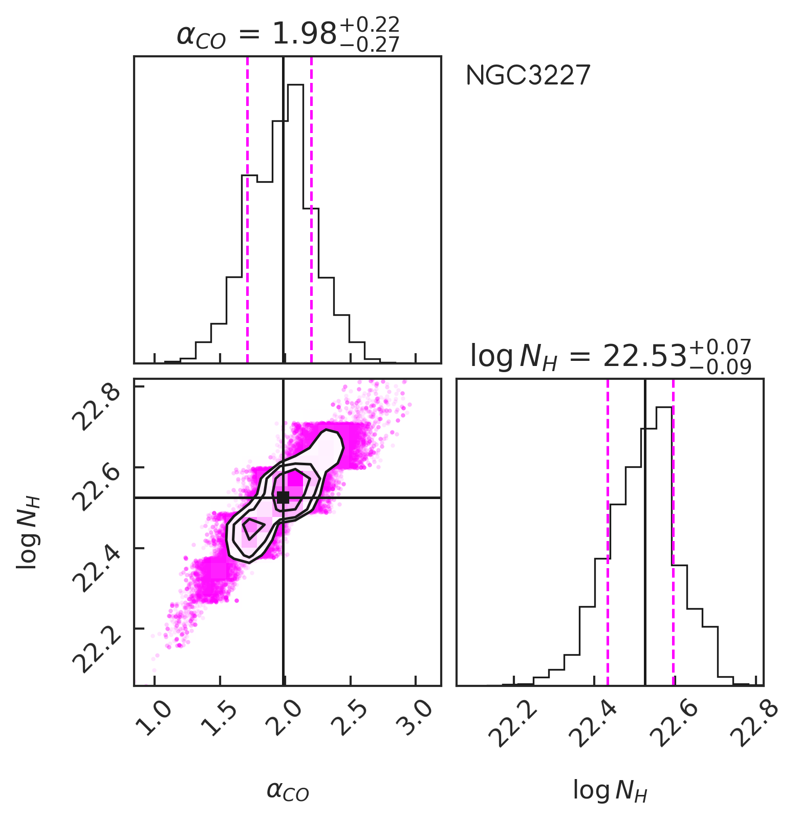
Figure 8: Corner plot showing the marginalized posterior distributions of $\alpha_{\text{CO}}$ (in M_⊙ (K km s^-1 pc²)^-1) and $N_{\text{H}}$ (in cm^-2) for the galaxy NGC 3227. The contours represent $(1,1.5,2)\sigma$ levels for the 2D distribution. The best-fitting parameters and the $16^{\text{th}}$ and $84^{\text{th}}$ percentiles are plotted with solid black lines and square and dashed magenta lines, respectively.

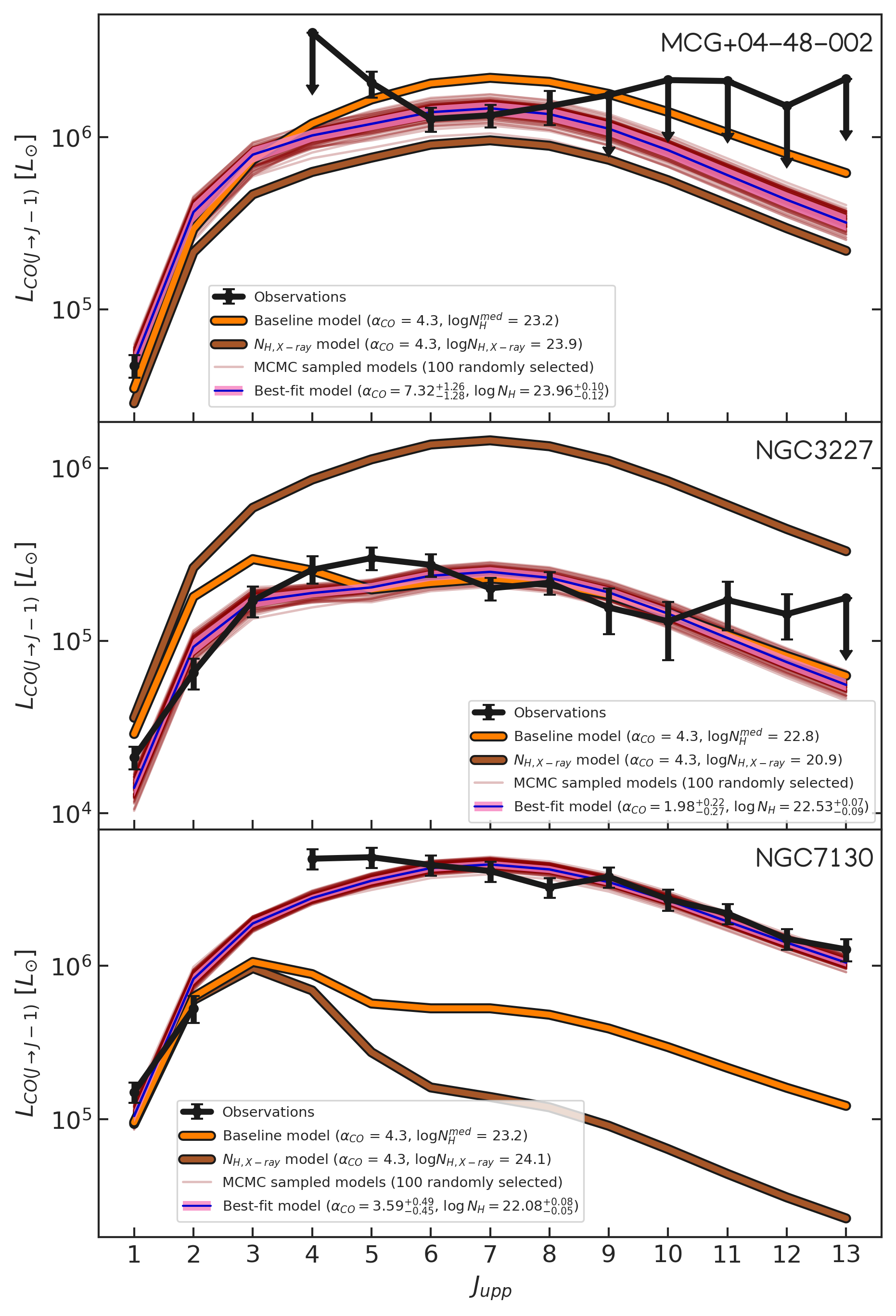
Figure 9: The modelled CO SLEDs of 3 galaxies (from the top to the bottom panel: MCG+04$-$48$-$002, NGC 3227 and NGC 7130) of our sample, in physical units of $L_{\odot}$. For each panel, the black line is the observed CO SLED (with downward arrows indicating censored data points), and the orange, brown, red, and pink lines are the modelled CO SLEDs: our baseline model without fitting any free parameter and with a negligible $N_{\text{H}}(r)$, the baseline model with a constant $N_{\text{H,X-ray}}$ derived by modelling the absorption of X-rays, 100 MCMC modelled SLEDs randomly picked from the parameters posterior distributions, and the best-fit model covering the $1\sigma$ spread of such distributions, respectively. The $x$-axis represents the upper rotational quantum number $J$ of each CO line, from CO($1-0$) to CO($13-12$).

In Appendix C, together with observed and modelled CO SLEDs for all the galaxies, we also plot the relative (i.e. normalized to the best-fit model) residuals between observed data and best-fit model. We find relative residual values $\geq 2$ for at least two detected CO lines in 4 galaxies: IRAS 20551$-$4250, Mrk 231, NGC 4151, and NGC 4388. Apart from NGC 4388, which has a very peculiar CO SLED shape that our model is not able to reproduce, for the other three galaxies our model fails to reach such high luminosities for the high-$J$ lines. This may be due to an additional source of excitation (other than FUV and X-ray flux), as shocks or cosmic rays. In fact, IRAS 20551$-$4250 and Mrk 231 are known to host powerful CO outflows, with velocities up to 500 and 700 km s^-1, respectively (Lutz et al., 2020). NGC 4388 has also a detected CO outflow, reaching 150 km s^-1 (Domínguez-Fernández et al., 2020), while for NGC 4151 we only have a detected H₂ outflow travelling at 300 km s^-1 (May et al., 2020). It is tempting to intepret these results as evidences of AGN mechanical feedback on CO excitation, but this is beyond the purpose of this work.

The best-fit $\alpha_{\text{CO}}$ and $N_{\text{H}}$, together with the $1\sigma$ spread of their posterior distributions, are listed, for each galaxy, in Table 2, together with the molecular mass within a $2r_{\text{CO}}$ radius (recalculated with the best-fit $\alpha_{\text{CO}}$).

4.3 Three examples of modelled galaxies

In Figure 9 we show the comparison between the observed CO SLED and that resulting from the "Baseline", "Best-fit", and "$N_{\text{H, X-ray}}$" modelling, where the "Best-fit" model is calculated with the $\pm 1\sigma$ values of the ($\alpha_{\text{CO}}$, $\log N_{\text{H}}$) posterior distributions. We show three sample galaxies: MCG+04$-$48$-$002, NGC 3227 and NGC 7130, chosen to be representative (due to the spread of their best-fit parameters) of the results obtained by means of our fitting procedure, with best-fit median values $\alpha_{\text{CO}}=[7.32,\,1.98,\,3.59]$ M_⊙ (K km s^-1 pc²)^-1, respectively, and $N_{\text{H}}=[10^{23.96},\,10^{22.53},\,10^{22.08}]$ cm^-2, respectively. In Appendix C we gather the observed and theoretical CO SLEDs for the whole galaxy sample.

MCG+04$-$48$-$002 (top panel of Figure 9) has very similar "$N_{\text{H, X-ray}}$", "Baseline" and "Best-fit" CO SLEDs, due to their similar $N_{\text{H}}$ values. The effect of a high $N_{\text{H}}$ on the CO SLED is visible especially at high $J$. The effect of changing $\alpha_{\text{CO}}$ (by a factor of $\sim 80\%$) is evident by comparing the "$N_{\text{H, X-ray}}$", and "Best-fit" CO SLEDs.

In NGC 3227 (middle panel of Figure 9) we can notice the difference between the "Baseline" and "Best-fit" CO SLEDs due to different $\alpha_{\text{CO}}$ and $N_{\text{H}}$: a higher $\alpha_{\text{CO}}$ would boost the luminosity of all the CO lines, but a higher $N_{\text{H}}$ decreases the high-$J$ lines, exposing a typical PDR bump in the low-$J$s (cfr. Figures 3 and 4). The "$N_{\text{H, X-ray}}$" SLED is very bright due to its low $N_{\text{H, X-ray}}$, which boosts the XDR emission.

NGC 7130 (bottom panel of Figure 9) has instead three very different modelled CO SLEDs. In the "Baseline" and "$N_{\text{H, X-ray}}$" models we can clearly see the PDR bump at low-$J$, due to the high $N_{\text{H}}$ which absorbs the X-rays. The higher $N_{\text{H, X-ray}}$ makes its SLED to dramatically decrease towards the high-$J$ lines, where the XDR emission is dominant. The "Best-fit" CO SLED has instead a lower PDR component due to its low $\alpha_{\text{CO}}=3.59$, which better reproduces the observed CO SLED.

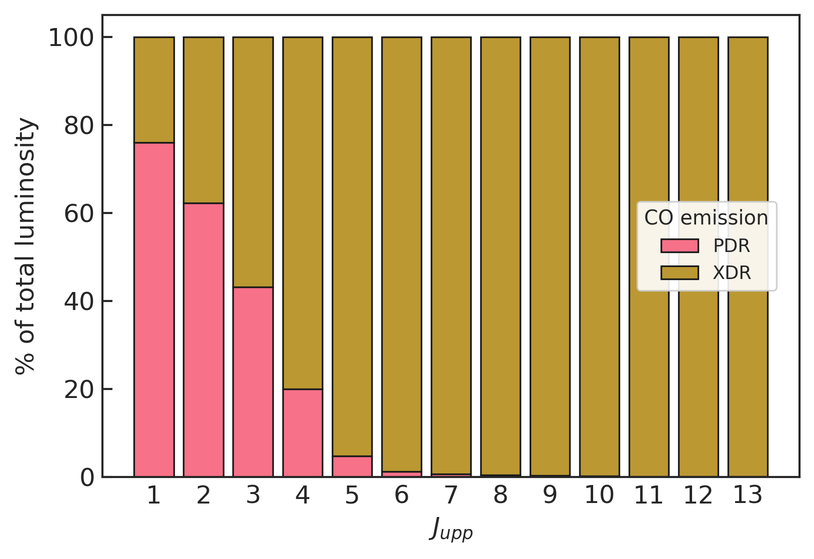
Figure 10: Bar plot showing the relative percentage to the total modelled luminosity of PDR (pink side) and XDR (brown side) emission for each analyzed CO line, from CO($1-0$) to CO($13-12$).

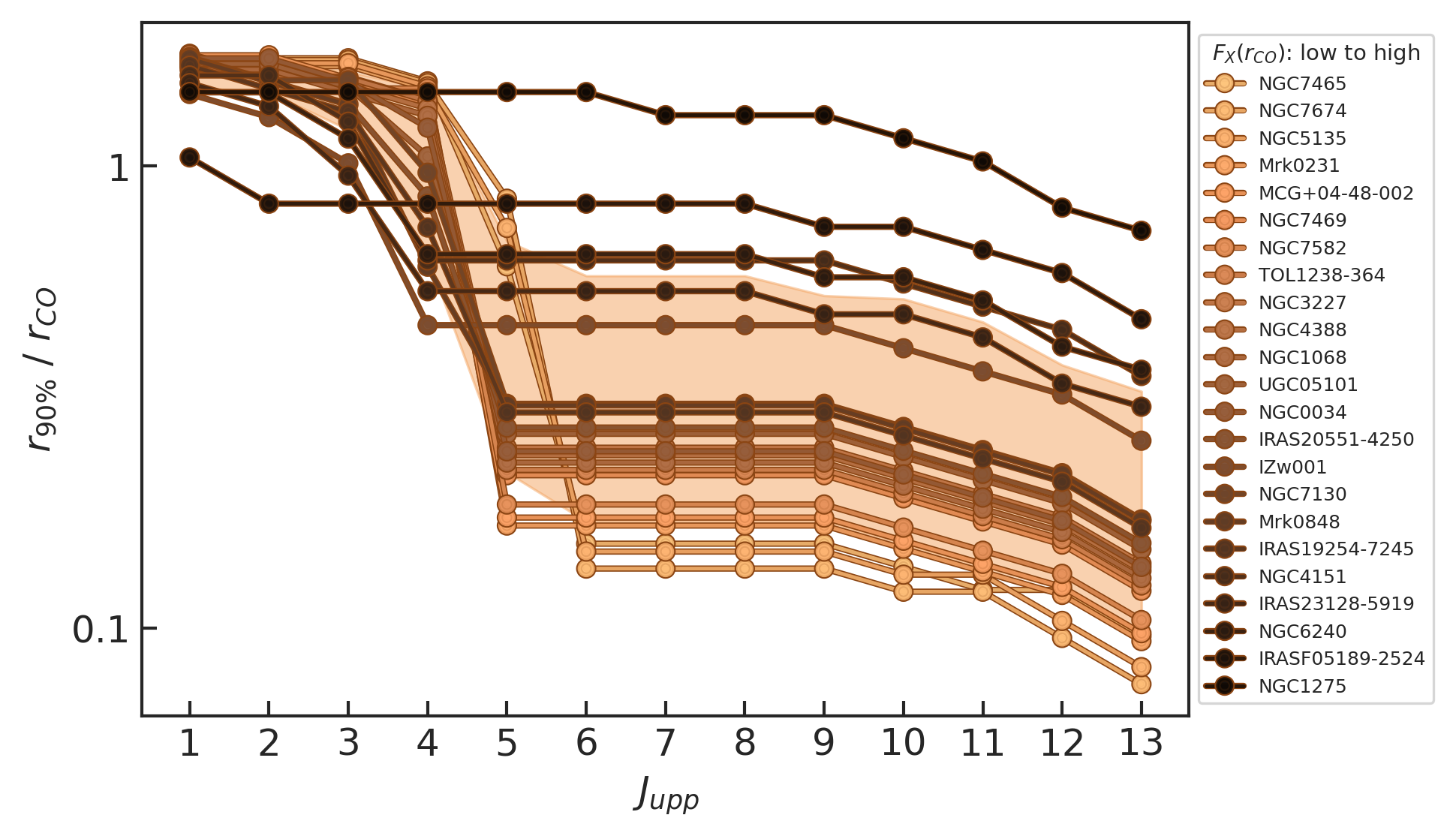
Figure 11: Galactocentric radius at which the luminosity of a given CO transition reaches $90\%$ of the total value for our sample of galaxies, divided by their $r_{\text{CO}}$. The filled circles, linked with solid lines, mark the $r_{90\%}$ for every galaxy, color-coded according to their $F_{\text{X}}(r_{\text{CO}})$, while the brown shaded area represents the values between $16\%$ and $84\%$ of the radii distributions for our sample.

4.4 PDR vs. XDR emission

In Figure 10 we plot the relative importance of PDR and XDR emission as a function of $J$ for our galaxy sample as resulting from the "Best-fit" model. It is remarkable the fact that from CO($4-3$) going upwards the CO luminosity is almost all due to XDR emission, even after taking into account the effect of X-ray flux attenuation with a best-fit $N_{\text{H}}$. This confirms what is shown in Figure 3 for single molecular clumps, and in Figure 4 for single GMCs, i.e. the XDR models dominate the overall CO luminosity, with the exception of the low-$J$ lines. These results are extensively discussed in Section 5.3.

4.5 The CO SLED radial build-up

Since we modelled the GMC distribution and their CO emission as a function of galactocentric radius, we can study the spatial distribution of different CO lines. In Figure 11 we plot the radius at which the luminosity of a given CO transition reaches $90\%$ of the total value for our sample of galaxies, $r_{90\%}$. It is immediate to see that there is a separation between low-$J$ lines, dominated by PDR emission (Figure 10), which emit up to several kpc (i.e. through the whole star-forming galaxy disc), and mid- and high-$J$ lines, dominated by XDR emission, which emit most of their luminosity within $r=1$ kpc. The spread in radii for a given CO line is due to the different sizes of the studied galaxies, but also, at least for the mid-/high-$J$, to the different incident $F_{\text{X}}$: a higher $F_{\text{X}}$ indeed produces a larger XDR emission (as in Meijerink & Spaans, 2005).

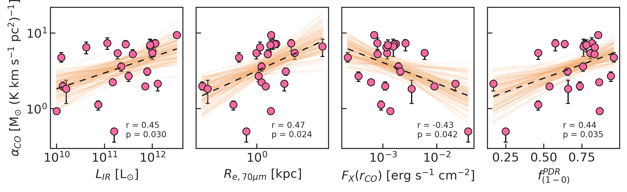
Figure 12: Scatter plot of best-fit $\alpha_{\text{CO}}$ (on the $y$-axis) against, from left to right, the total IR luminosity, the effective radius of the 70 $\mu$m maps, the PDR fraction of the total CO($1-0$) modelled emission, and the X-ray flux at $r_{\text{CO}}$, for the whole galaxy sample. The dashed black line is the regression fit between the quantities on the $x$ and $y$ axes, and the brown lines are 100 bootstrapped fits, which highlight the confidence interval of the regression fit. The Pearson correlation coefficient $r$ and the $p$-value appear on every panel on the bottom right.

5 Discussion

In this section we discuss the implications of the derived values of the CO-to-H₂ conversion factor $\alpha_{\text{CO}}$ and the gas column densities $N_{\text{H}}$ for our galaxy sample. Finally, we discuss about the relative importance of PDRs and XDRs to the CO luminosity.

5.1 The CO-to-H₂ conversion factor $\alpha_{\text{CO}}$

The best-fit procedure returns reasonable values for $\alpha_{\text{CO}}$. We find a median value of $\alpha_{\text{CO}}=4.8^{+2.4}_{-2.8}$ M_⊙ (K km s^-1 pc²)^-1, which is similar to the Milky-Way adopted value. Less than a third (8/24) of our sample has a ULIRG-like $\alpha_{\text{CO}}=1.8^{+1.3}_{-0.8}$ M_⊙ (K km s^-1 pc²)^-1 (Herrero-Illana et al., 2019; Pérez-Torres et al., 2021), even though only one of them (IRAS F05189$-$2524) is a ULIRG, and four (Mrk 848, NGC 5135, NGC 6240, and NGC 7674) are LIRGs.

For some targets we have independent measures of $\alpha_{\text{CO}}$ from the literature to compare with. By modelling the gas dynamics, Fei et al. (2023) found, for I Zw 1, $\alpha_{\text{CO}}=1.6\pm 0.5$ M_⊙ (K km s^-1 pc²)^-1, which is lower than our result ($\alpha_{\text{CO}}=6.6\pm 1.7$ M_⊙ (K km s^-1 pc²)^-1); however, their analysis is limited to the central 1 kpc, whereas our model extends up to $2r_{\text{CO}}$ (i.e. 5.6 kpc for I Zw 1). By comparing gas and dust emission, García-Burillo et al. (2014) found values in the range $0.43-1.43$ M_⊙ (K km s^-1 pc²)^-1 for the central 700 pc of NGC 1068 (whereas we find $\alpha_{\text{CO}}=5.4^{+0.9}_{-0.5}$ M_⊙ (K km s^-1 pc²)^-1 up to a diameter of 4.9 kpc). In NGC 6240, the quiescent gas and the outflowing one have different $\alpha_{\text{CO}}=3.2\pm 1.8$ M_⊙ (K km s^-1 pc²)^-1 and $\alpha_{\text{CO}}=2.1\pm 1.2$ M_⊙ (K km s^-1 pc²)^-1, respectively (Cicone et al., 2018): our value for this galaxy ($\alpha_{\text{CO}}=2.0\pm 0.1$ M_⊙ (K km s^-1 pc²)^-1) is closer to the outflowing gas, which is where the bulk of the molecular mass is, according to Cicone et al. (2018). The circumnuclear region (up to a 175 pc radius) of NGC 7469 has a $\alpha_{\text{CO}}$ between 1.7 and 3.4 M_⊙ (K km s^-1 pc²)^-1 according to Davies et al. (2004). Our model gives a higher result ($\alpha_{\text{CO}}=5.3^{+0.5}_{-0.7}$ M_⊙ (K km s^-1 pc²)^-1) but it is derived for the molecular gas extending up to a 4.7 kpc radius.

Surprisingly, we find a positive, moderate (Pearson coefficient $r=0.45$, $p=0.03$), correlation between $\alpha_{\text{CO}}$ and the total IR luminosity $L_{\text{IR}}$, as shown in the first panel of Figure 12. The value of $\alpha_{\text{CO}}$ is predicted to decrease for higher gas temperatures, hence for starburst galaxies as (U)LIRGs (Bolatto et al., 2013). However, high gas and column densities are expected to increase $\alpha_{\text{CO}}$: for example, Teng et al. (2023) found $\alpha_{\text{CO}}$ to increase in the central region of local barred galaxies due to the high CO optical depth, which they find to be a more dominant driver than the gas temperature. A limit of the present analysis is the fact that we used a single $\alpha_{\text{CO}}$ for every radius, while it is likely to vary with different local conditions, as metallicity, temperature, density and optical depth (Bolatto et al., 2013; Teng et al., 2023). Another important point to make is that our (U)LIRGs (17/24 galaxies have $L_{\text{IR}}\geq 10^{11}$ L_⊙) are AGN, so that a fraction of the IR luminosity is due to AGN activity rather than SF (e.g. Nardini et al., 2010; Alonso-Herrero et al., 2012). For example, the largest value we derive is $\alpha_{\text{CO}}=9.41$ M_⊙ (K km s^-1 pc²)^-1 for Mrk 231, the only quasar of our sample, with $L_{\text{IR}}=10^{12.5}$ L_⊙, the highest of our sample.

We also find $\alpha_{\text{CO}}$ to correlate with the effective radius $R_{e,70\mu m}$ of the 70 $\mu$m emission ($r=0.47$, $p=0.02$, second panel of Figure 12). These radii result from the Sersic fit on the Herschel maps analyzed in E22. No significant correlation ($r=-0.12$, $p=0.58$) shows up instead between $\alpha_{\text{CO}}$ and $r_{\text{CO}}$: this means that the optical and molecular radii ($r_{\text{CO}}=0.17\,r_{25}$) do not affect the CO-to-H₂ conversion factor, while it seems influenced by the size of the star-forming region (traced by the 70 $\mu$m emission in our analysis). We do also find $L_{\text{IR}}$ and $R_{e,70\mu m}$ to strongly correlate between each other ($r=0.72$, $p=8\times 10^{-5}$), so it is possible that only one of the two correlations is actually meaningful. There is no significant correlation ($r=0.13$, $p=0.56$) between $\alpha_{\text{CO}}$ and the median $G_{0}$ listed in Table 2, or the $G_{0}(R_{e,70\mu m})$, so it seems $G_{0}$ is not the main driver of the $\alpha_{\text{CO}}$ variation.

Some clues can come from the way we implemented $\alpha_{\text{CO}}$ in our model, i.e. as a normalization factor of the "Best-fit model". A bright IR galaxy has also bright CO emission at every $J$ (e.g. Kamenetzky et al., 2016). However, there is complex interplay between the combined effects of $\alpha_{\text{CO}}$ and $N_{\text{H}}$ in our model. For example, MCG+04$-$48$-$002 (top panel of Figure 9) has a high $\alpha_{\text{CO}}=7.32$ M_⊙ (K km s^-1 pc²)^-1, even though the "Baseline model", made with a lower $\alpha_{\text{CO}}$, is brighter for some CO lines, and this is due to the high $N_{\text{H}}$ that we derived for this galaxy, which suppresses the XDR emission. We do not find ($r=0.28$, $p=0.20$) a convincing correlation between the two best-fit parameters ($\alpha_{\text{CO}}$, $N_{\text{H}}$), but we do find (third panel of Figure 12) an anti-correlation ($r=-0.43$, $p=0.04$) between $\alpha_{\text{CO}}$ and $F_{\text{X}}$ measured at a distance $r_{\text{CO}}$ from the AGN, and obscured with the best-fit $N_{\text{H}}$: a high $F_{\text{X}}$ is indeed expected to boost the XDR CO emission, hence lowering $\alpha_{\text{CO}}$.

In the last panel of Figure 12, we show a positive, moderate ($r=0.44$, $p=0.04$), correlation between $\alpha_{\text{CO}}$ and the PDR fractions to the total CO($1-0$) modelled emission. For some galaxies (e.g. MCG+04$-$48$-$002, which has a high $f^{(1-0)}_{\text{PDR}}=0.81$ – see Table 2) this is due to the combined effect of $\alpha_{\text{CO}}$ and $N_{\text{H}}$: a high $N_{\text{H}}$ suppresses the XDR emission, so that a high $\alpha_{\text{CO}}$ is needed to boost the otherwise low PDR emission and increase the likelihood.

We stress that the characterization of a class of objects (local AGN as in our study) or even more of individual galaxies by constraining galaxy properties such as $\alpha_{\text{CO}}$, is in line with some recent studies (e.g., Ellison et al., 2021; Casasola et al., 2022; Salvestrini et al., 2022; Thorp et al., 2022). These works highlight the heterogeneity of properties of the local galaxies, in addition to provide observational constraints to theoretical models and for high-redshift studies.

5.2 The X-ray attenuation column density

Taking into account the $1\sigma$ uncertainty, we find non-negligible (i.e. $N_{\text{H}}>10^{22}$ cm^-2, see Equation 8) X-ray attenuation for most (14/23 galaxies) of our sample. The median is $\log(N_{\text{H}}/\text{cm}^{-2})=22.1^{+1.6}_{-0.1}$, and the range [$10^{22},10^{24}$] cm^-2. By comparison the column density derived from the X-ray SED, for 20/23 galaxies, has median $\log(N_{\text{H, X-ray}}/\text{cm}^{-2})$ $=23.7^{+0.5}_{-2.0}$ and range [$10^{20.5},10^{25}$] cm^-2.

Although our best-fit $N_{\text{H}}$ approximately has the same range of $N_{\text{H, X-ray}}$, the two values do not correlate (Figure 7). This uncorrelation can be due to the different locations of the X-ray absorbers: in the case of $N_{\text{H, X-ray}}$, the X-ray flux is attenuated by gas clouds along the line of sight only, while the $N_{\text{H}}$ we derive is due to clouds between the AGN and the GMCs in the whole galaxy volume (i.e. considering multiple lines of sight).

Lately, more complex models of X-ray absorption are leading to different estimates of $N_{\text{H}}$, measuring the obscuration along the line of sight plus a reflective component from the nuclear torus (Yaqoob, 2012; Esparza-Arredondo et al., 2021). Several works targeting local AGNs show that these different $N_{\text{H}}$, both estimated from the X-ray SED, fail to correlate between each other (Torres-Albà et al., 2021; Sengupta et al., 2023).

García-Burillo et al. (2021) compared instead different estimates of $N_{\text{H}}$, from X-ray absorption, and from high-resolution (7-10 pc) ALMA CO observations, for a sample of 19 local Seyferts, finding similar median values but with a large dispersion around the 1:1 line. As our estimates of Figure 7, they also find less absorbed galaxies (with $N_{\text{H,X-ray}}<10^{22}$ cm^-2) to systematically lie above the 1:1 line, and vice versa. This could be expected if, in less absorbed galaxies, $N_{\text{H,X-ray}}$ is dominated by gas clouds smaller than our spatial resolution, which is dictated by the diameter of our smallest modelled GMC (3 pc, see Table 1).

It is believed that, at least in local AGNs, most of the obscuration is due to the nuclear torus rather than gas on galactic scales (see Hickox & Alexander 2018 for a recent review, and Gilli et al. 2022 for high-redshift systems). However, the orientation, filling factor and opening angle of the torus are all important quantities that affect the measurement of $N_{\text{H, X-ray}}$. With our analysis we give a way to measure the attenuation of AGN obscuration on the molecular gas in all the possible directions.

5.3 PDR vs. XDR emission

As shown in Figures 3 and 4, the CO luminosity is dominated, for our modelled clumps and GMCs, by XDR emission, at least at $J>3$. We find the same by fitting the observed CO SLEDs (Figure 10). The fact that high-$J$ lines need X-rays to be radiatively excited is well known and studied (Bradford et al., 2009; van der Werf et al., 2010; Rosenberg et al., 2015; Kamenetzky et al., 2017), however this is the first time a detailed study of CO emission, coming from different gas sizes (clumps, GMCs), produces this same result. The majority of the studies have found, so far, CO excitation to be consistent with PDRs up to CO($6-5$) (van der Werf et al., 2010; Hailey-Dunsheath et al., 2012; Pozzi et al., 2017). One notable exception is the work by Mingozzi et al. (2018), where their fiducial model for the CO SLED of NGC 34 has a XDR component which starts dominating the luminosity at $J_{\text{upp}}=3$.

All these studies used a combination of two or three PDR and XDR components, each with a single density and incident flux. To be able to reproduce PDR emission consistent with observations at mid-/high-$J$, these models need very high gas densities ($n_{\text{H}}\gtrsim 10^{5}$ cm^-3), more typical of high-redshift, turbulent star-forming regions (Calura et al., 2022). The mass fraction of such dense clumps within the modelled GMCs is $\sim 2\%$, being most of the molecular mass in the range $[10^{2},10^{4}]$ cm^-3, where only XDRs are able to emit significant high-$J$ CO emission (see also Figure 4). This also confirms the findings of E22, i.e. that only unlikely extreme gas densities PDR models can reproduce the CO emission.

As a caveat, we note that our model does not include (i) variations in the cosmic ray ionisation rate (CRIR), and (ii) the effect of shocks. It is known that both high cosmic-ray fluxes (Vallini et al., 2019; Bisbas et al., 2023) and shocks (Meijerink et al., 2013; Mingozzi et al., 2018; Bellocchi et al., 2020) influence the CO SLED, especially the high-$J$ lines. Further developments of our model may be able to include a varying CRIR and the treatment of large scale shocks, as in the case of galaxies with winds and outflows (García-Burillo et al., 2014; Morganti et al., 2015; Fiore et al., 2017; Speranza et al., 2022) or mergers (Ueda et al., 2014; Larson et al., 2016; Ellison et al., 2019).

6 Conclusions

We have presented a new physically-motivated model for computing the CO SLED in AGN-host galaxies, which takes into account the internal structure of GMCs, the radiative transfer of external FUV and X-ray flux on the molecular gas, and the mass distribution of GMCs within a galaxy volume. The assumptions are that the molecular clumps in a GMC follow a log-normal density distribution, the clumps size is equal to their Jeans radius, and that the GMC masses, in a galaxy, follow a power-law distribution. The model can predict the CO SLED of a galaxy from the radial profiles of molecular mass $M_{\text{mol}}(r)$, FUV flux $G_{0}(r)$ and X-ray flux $F_{\text{X}}(r)$. We also set two free parameters: the CO-to-H₂ conversion factor $\alpha_{\text{CO}}$, and the X-ray attenuation column density $N_{\text{H}}$. We have used Cloudy to predict the CO lines emission of clumps and GMCs, through a combination of PDR and XDR simulations, and by taking into account the observed radial profiles.

To test the validity of our model, we extracted, from the galaxy sample of E22, a sub-sample of 24 X-ray selected AGN-host galaxies with a well-sampled CO SLED. The sample represents a good variety of local ($z\leq 0.06$) moderately luminous ($10^{42}\leq L_{\text{X}}[\text{erg s}^{-1}]\leq 10^{44}$, $10^{10}\leq L_{\text{IR}}[\text{L}_{\odot}]\leq 10^{12.5}$) AGNs. We compared the CO SLEDs produced by our model with the observed ones, and we selected the best-fit $\alpha_{\text{CO}}$ and $N_{\text{H}}$ with a MCMC analysis for each galaxy. Our main results are here summarized:

• the best-fit procedure returned, for our galaxy sample, median values of $\alpha_{\text{CO}}=4.8^{+2.4}_{-2.8}$ M_⊙ (K km s^-1 pc²)^-1 and $\log(N_{\text{H}}/\text{cm}^{-2})=22.1^{+1.6}_{-0.1}$, where the lower and upper errors are the $16^{\text{th}}$ and $84^{\text{th}}$ percentiles, respectively; we find $\alpha_{\text{CO}}$ consistent with the Galactic value, and $N_{\text{H}}$ that do not correlate with $N_{\text{H, X-ray}}$;

• XDRs are fundamental to reproduce observed CO SLEDs of AGN-host galaxies, particularly for $J_{\text{upp}}\gtrsim 3$.

We argue that the larger importance of X-rays to the CO luminosity, with respect to other works in the literature, is mainly due to the fact that the majority of molecular gas mass in a galaxy is at $n_{\text{H}}\sim 10^{2}-10^{4}$ cm^-3. This conclusion comes from a physically-motivated structure for the molecular gas, rather than from single-density radiative transfer models.

The model predictions can be used to estimate $\alpha_{\text{CO}}$ in AGN-host galaxies, by constraining both the relative and absolute intensity of several CO lines. They can also be useful to estimate the effective attenuation of X-ray photons on the molecular gas in a spatially-resolved way, rather than only on the line-of-sight (i.e., $N_{\text{H, X-ray}}$).

Moving forward, the model is able to predict the emission of other molecular species, as HCN, HCO⁺, H₂, H₂O. These molecules have been increasingly used in detailed studies of local AGN (Butterworth et al., 2022; Eibensteiner et al., 2022; Huang et al., 2022). The model is also built to exploit a wealth of observed galaxy data, and compare different molecular lines spatially resolved by ALMA (as done with NGC 1068 in García-Burillo et al., 2019; Nakajima et al., 2023) with our model predictions.

Data Availability

We publicly release the code, called galaxySLED, on GitHub (https://federicoesposito.github.io/galaxySLED/). The data generated in this research will be shared on reasonable request to the corresponding author.

Appendix A Update of observed fluxes for our sample

Reviewing the data contained in E22, we have found a better source for one CO line luminosity in one galaxy. The CO($2-1$) of NGC 1275 was taken, in E22, from Salomé et al. (2011), which was converted to $303^{+8}_{-8}\times 10^{2}$ L_⊙. Since this flux was observed, in Salomé et al. (2011), from a very small nuclear region of NGC 1275, we wanted to improve the measurement by finding another observation with a larger beam. Lazareff et al. (1989) observed the CO($2-1$) emission with the IRAM-30m telescope, which has a full-width at half maximum (FWHM) of 10$\aas@@fstack{\prime\prime}$5, finding a larger CO($2-1$) luminosity of $15^{+3}_{-3}\times 10^{4}$ L_⊙. Throughout this paper we use this value, since it is the one with the larger beam we can find for this galaxy; in this way the CO($2-1$) beam is almost equal to the projected $r_{\text{CO}}$ of the galaxy: $r_{\text{CO}}=$ 10$\aas@@fstack{\prime\prime}$9.

Appendix B Radial profiles of galaxies

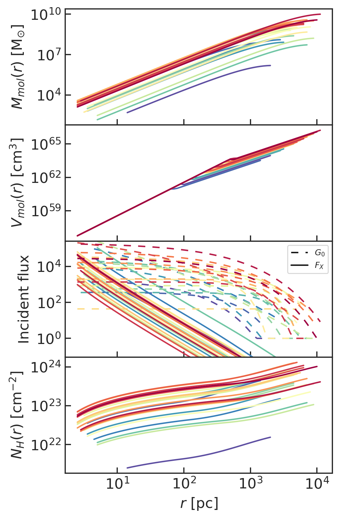
Figure 13: Radial profiles of our sample of 24 galaxies, sorted by their total molecular mass when measured with a Milky Way $\alpha_{\text{CO}}$. The four panels show, from top to bottom, the molecular mass $M_{\text{mol}}(r)$ (recalculated with the best-fit $\alpha_{\text{CO}}$), the molecular volume $V_{\text{mol}}(r)$, the incident fluxes $G_{0}(r)$ and $F_{\text{X}}(r)$, and the "Baseline model" column density $N_{\text{H}}(r)$. $G_{0}(r)$ and $F_{\text{X}}(r)$ are in $G_{0}$ and erg s^-1 cm^-2 units and they are plotted with dashed and solid lines, respectively. Colors are the same as Figure 5.

In Figure 13 we show the radial profiles of the molecular mass $M_{\text{mol}}(r)$, the volume $V_{\text{mol}}(r)$, the incident fluxes $G_{0}(r)$ and $F_{\text{X}}(r)$, and the intrinsic column density $N_{\text{H}}(r)$. $M_{\text{mol}}(r)$ has been recalculated with the best-fit $\alpha_{\text{CO}}$. The radial profiles all follow the Equations (5) $-$ (9).

Appendix C Observed and modelled CO SLEDs for the whole galaxy sample

Figures 14 - 36 show the "Baseline model", and "$N_{\text{H, X-ray}}$ model" for each galaxy of the sample with orange and brown lines, respectively. The observed CO SLED is plotted with a black line, with vertical bars representing measurement errors, and downward arrows indicating censored data points (i.e. upper limits). We randomly select, from the posterior distributions of the model parameters $\alpha_{\text{CO}}$ and $\log N_{\text{H}}$, 100 different modelled CO SLEDs, plotted in red. The blue lines and pink shadings, are the modelled CO SLEDs with the median and $1\sigma$ spread of the model parameters posterior distributions, respectively; we call "Best-fit model" the one with the median values of $\alpha_{\text{CO}}$ and $\log N_{\text{H}}$. For each galaxy, the bottom panels of Figures 14 - 36 show in black the relative residuals, calculated as the difference between observations and best fit model, divided by the latter; the best-fit model is the blue line (fixed at 0), with the $1\sigma$ spread in pink shading.

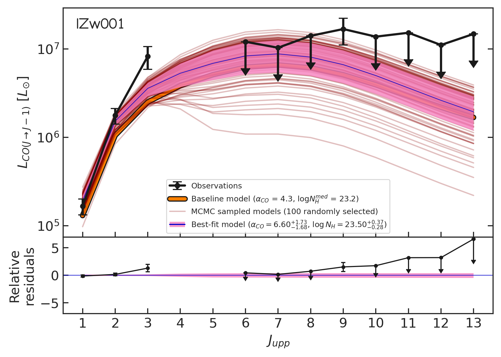
Figure 14: I Zw 1 (UGC 545) CO SLEDs.

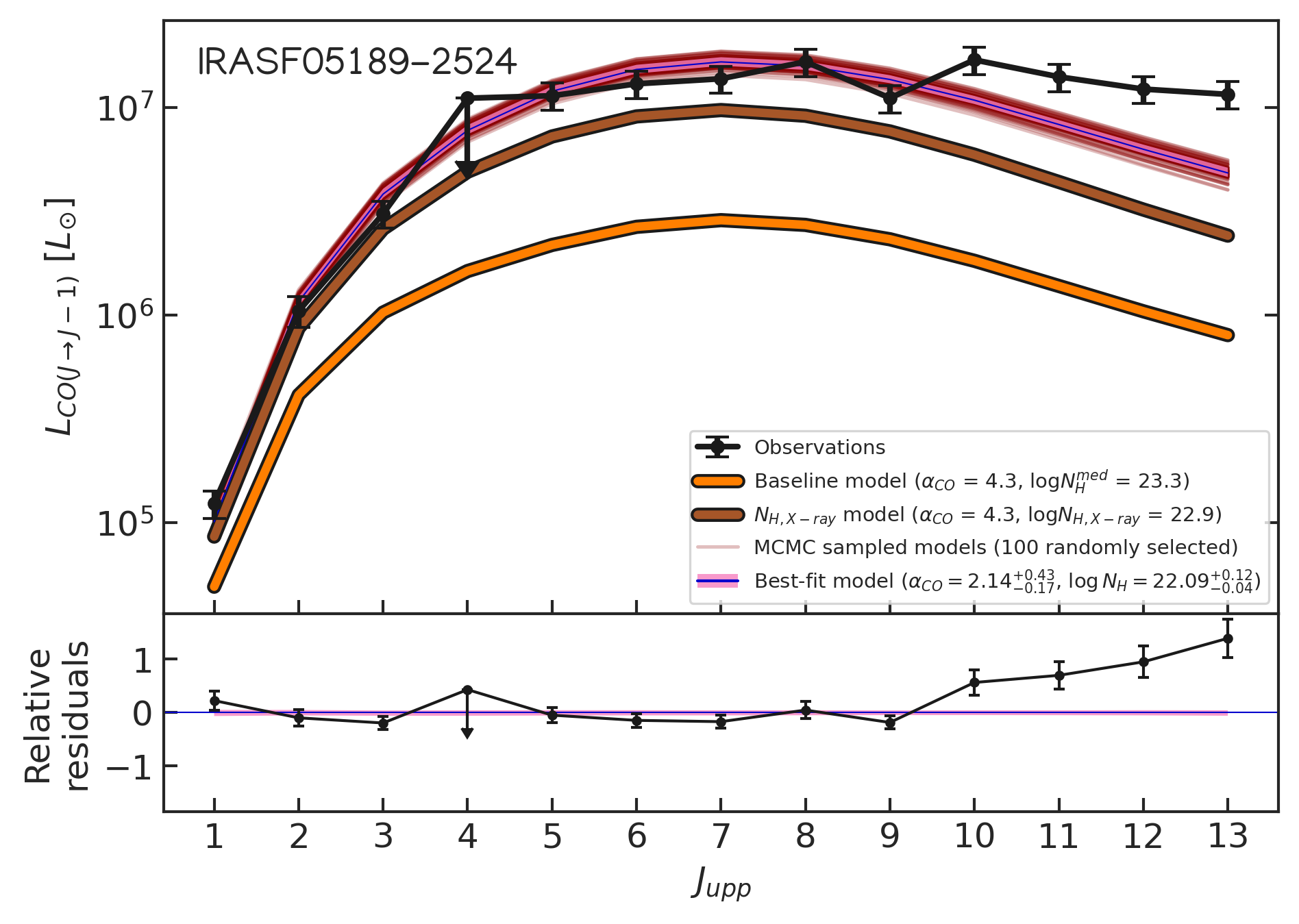
Figure 15: IRAS F05189$-$2524 CO SLEDs.

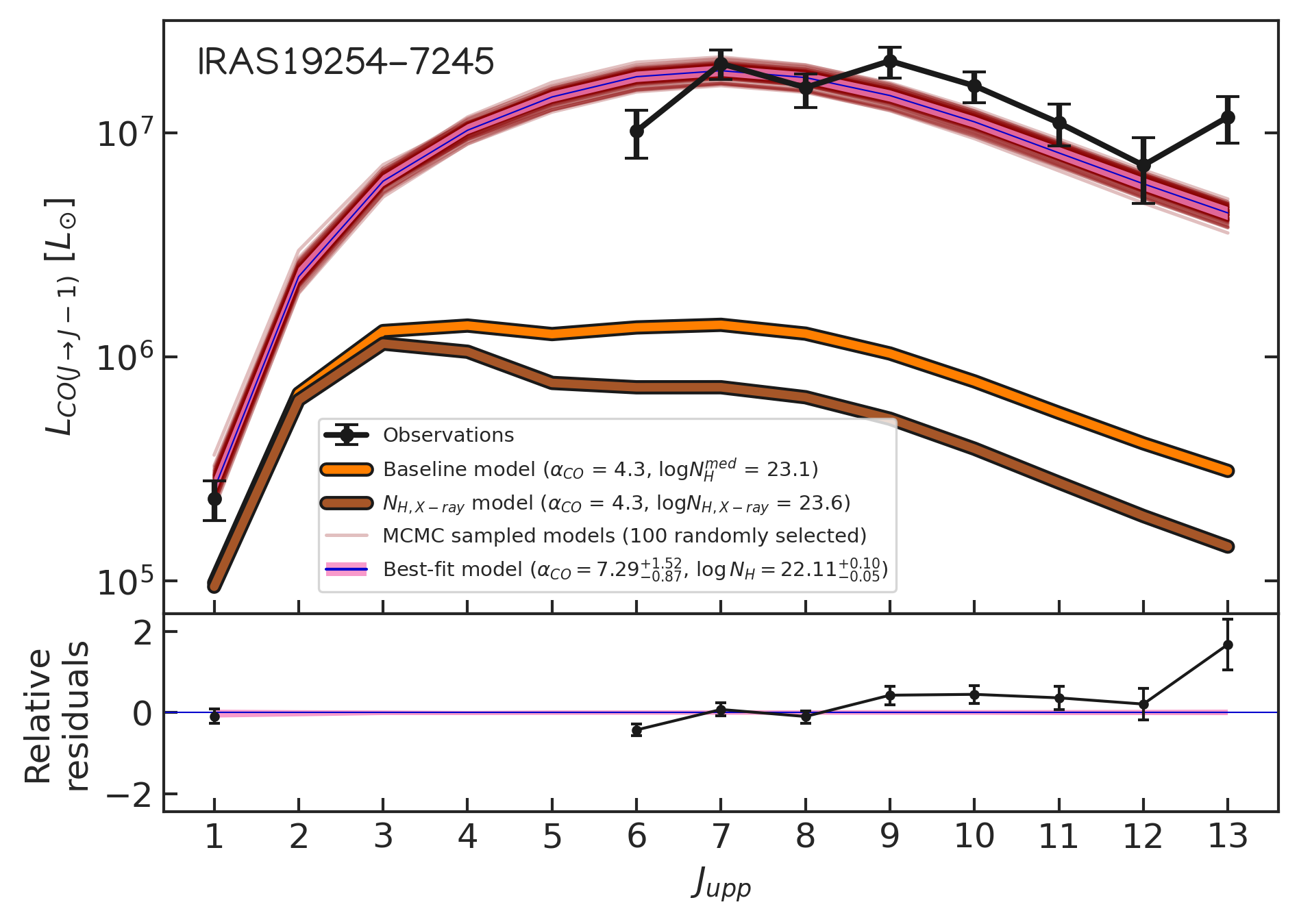
Figure 16: IRAS 19254$-$7245 (Superantennae) CO SLEDs.

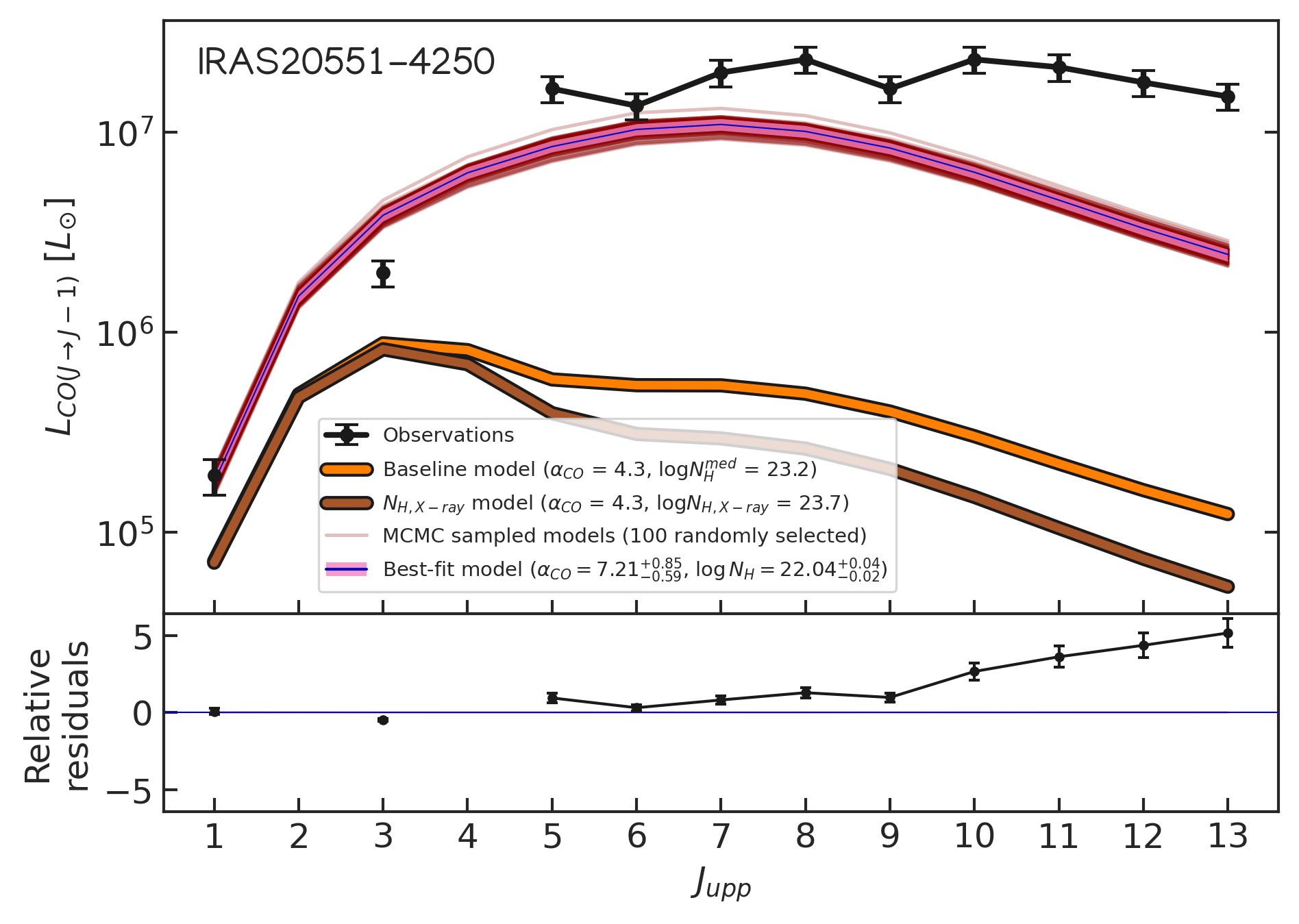
Figure 17: IRAS 20551$-$4250 (ESO 286$-$IG019) CO SLEDs.

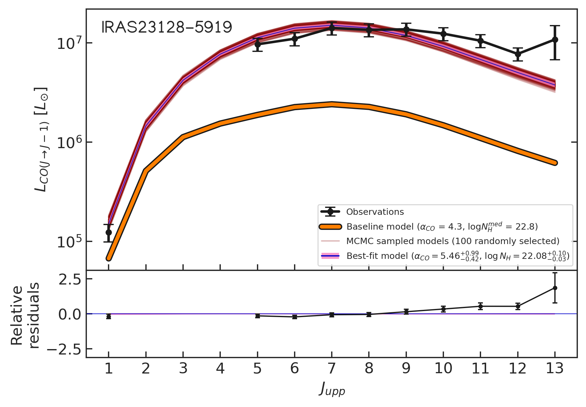
Figure 18: IRAS 23128$-$5919 (ESO 148$-$IG002) CO SLEDs.

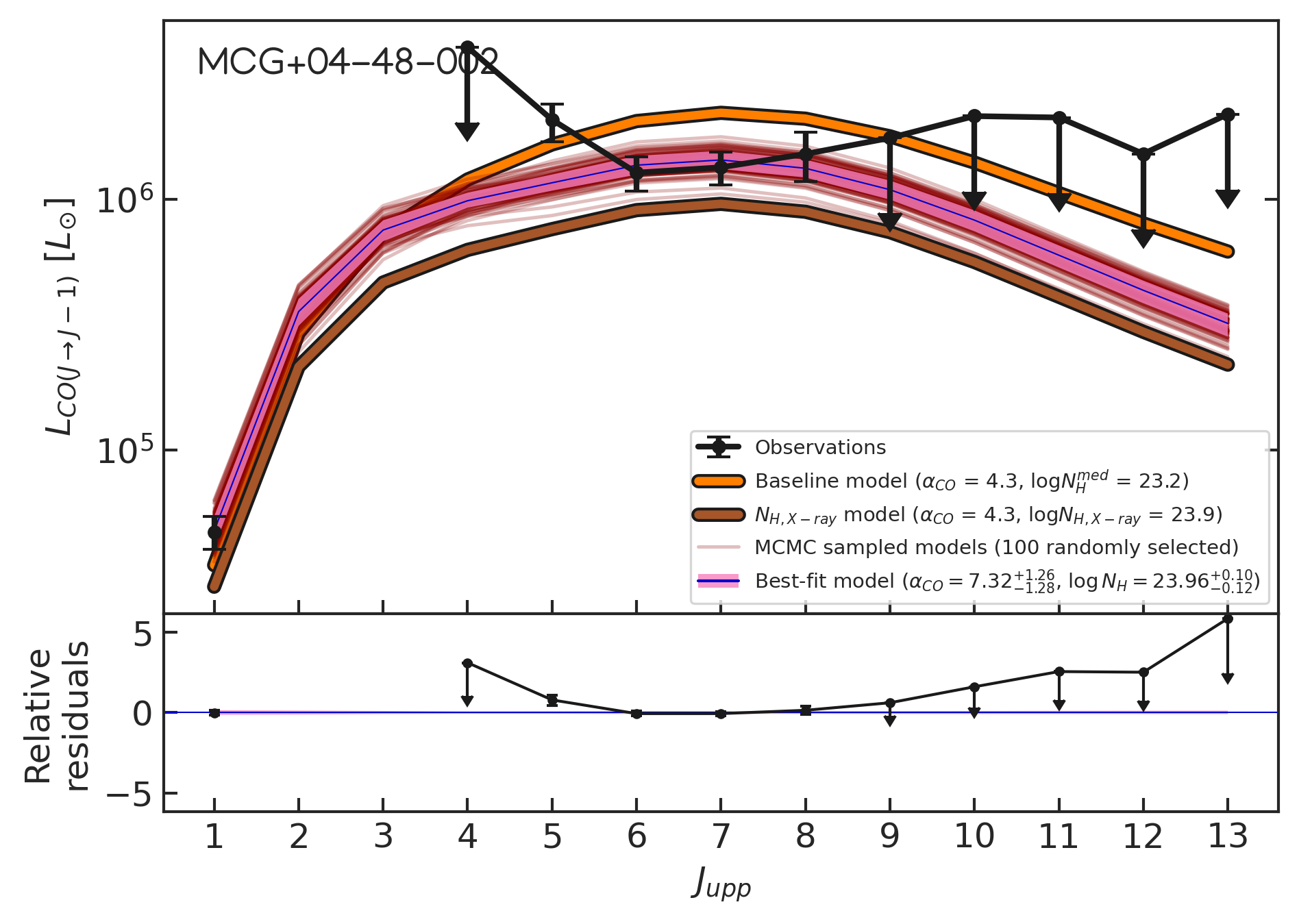
Figure 19: MCG +04$-$48$-$002 CO SLEDs.

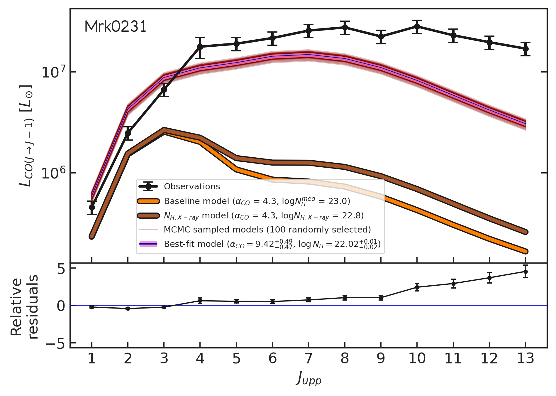
Figure 20: Mrk 231 CO SLEDs.

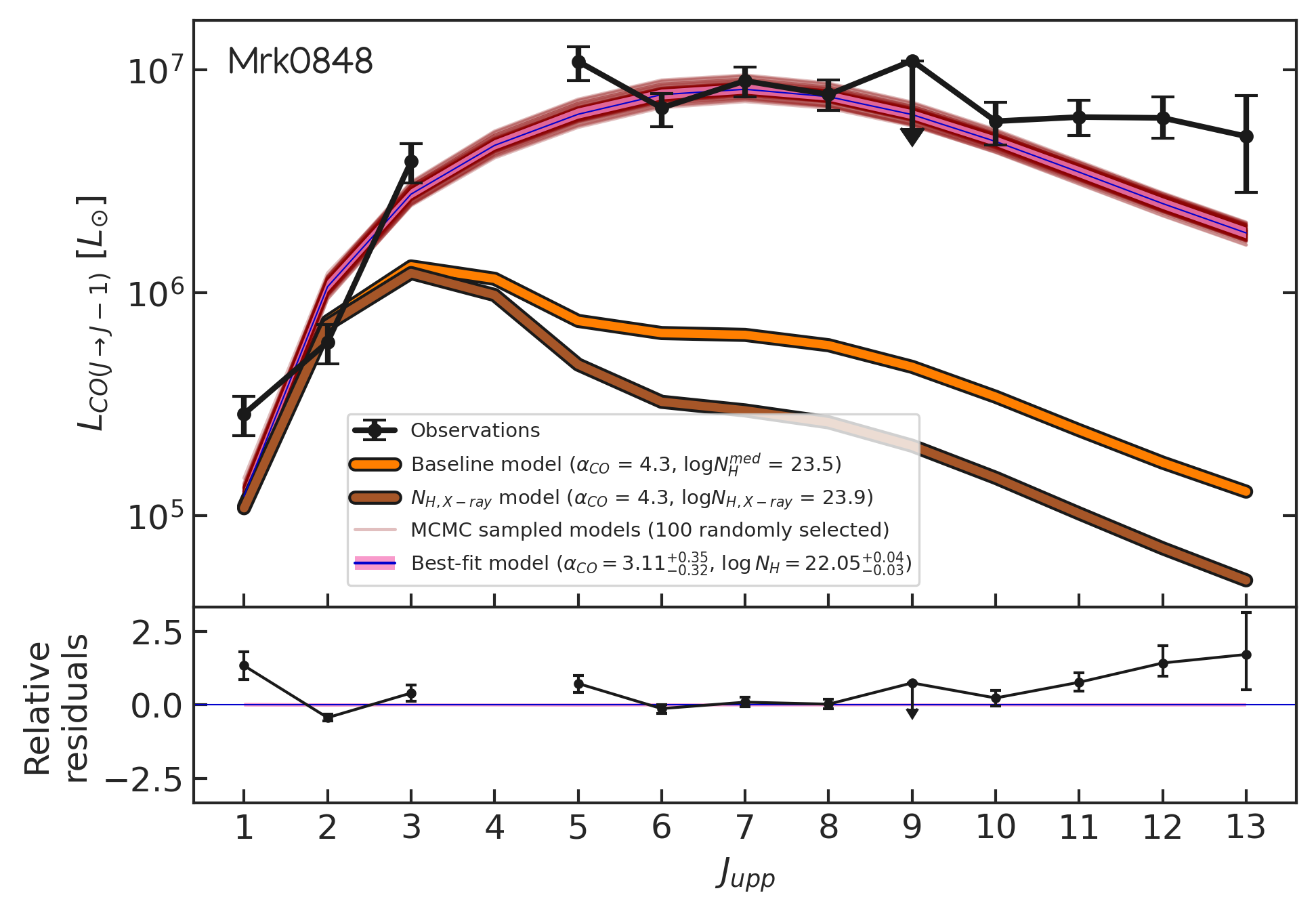
Figure 21: Mrk 848 (VV 705) CO SLEDs.

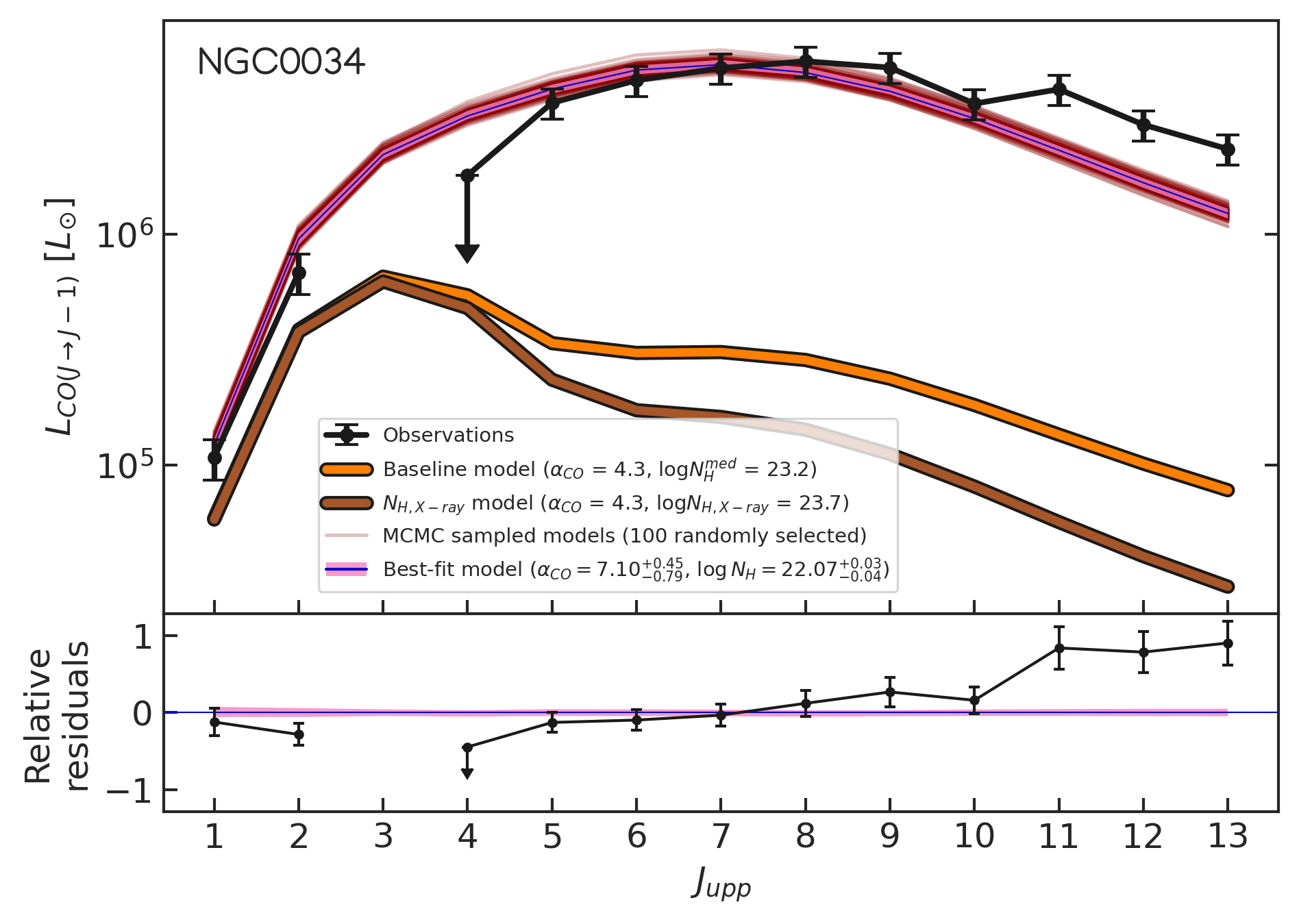
Figure 22: NGC 34 (Mrk 938) CO SLEDs.

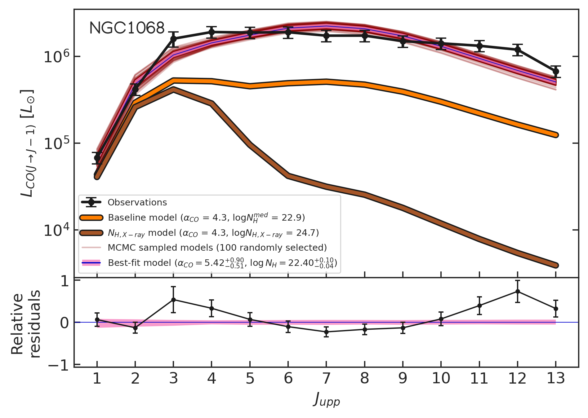
Figure 23: NGC 1068 (M77) CO SLEDs.

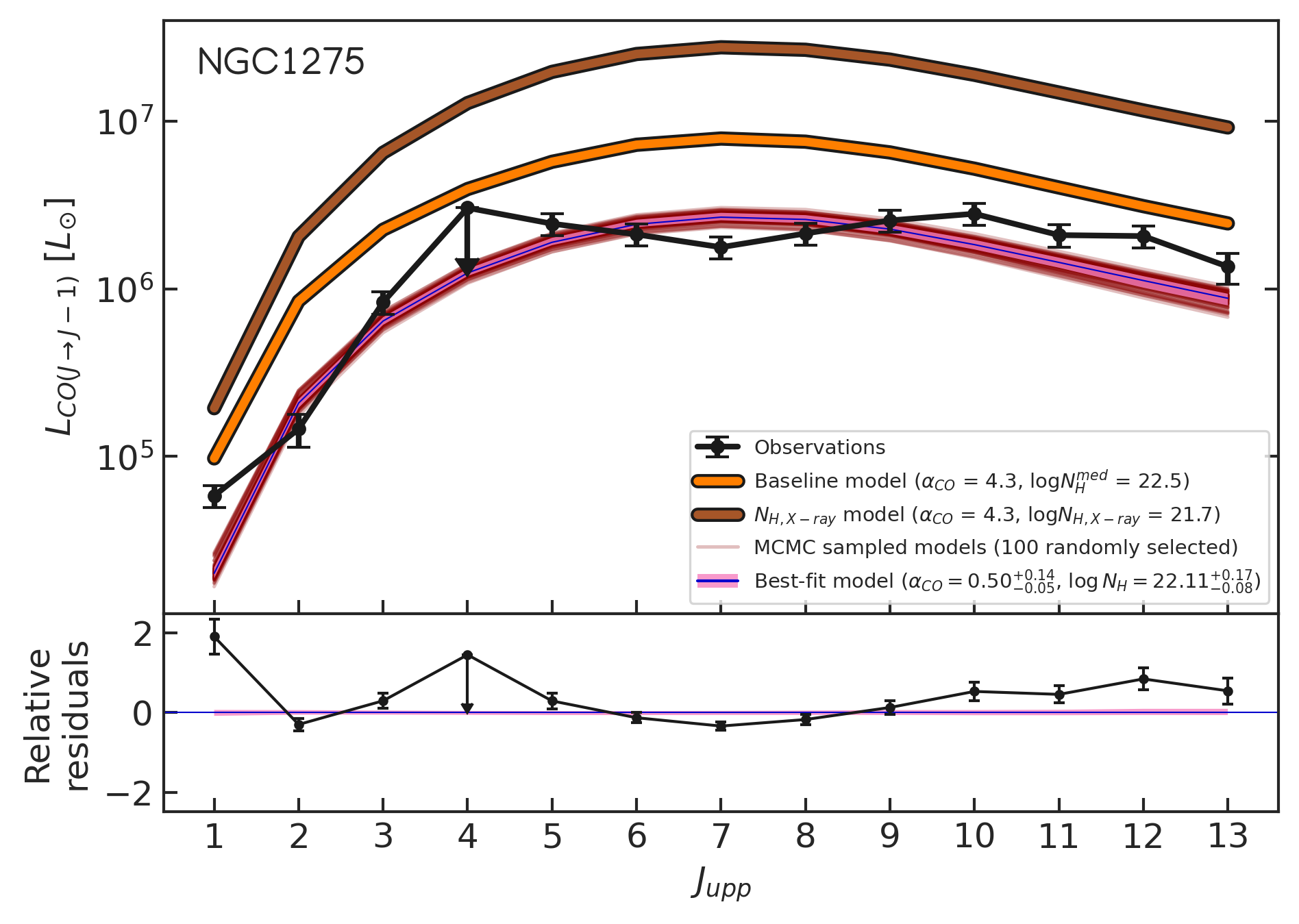
Figure 24: NGC 1275 (3C84, Perseus A) CO SLEDs.

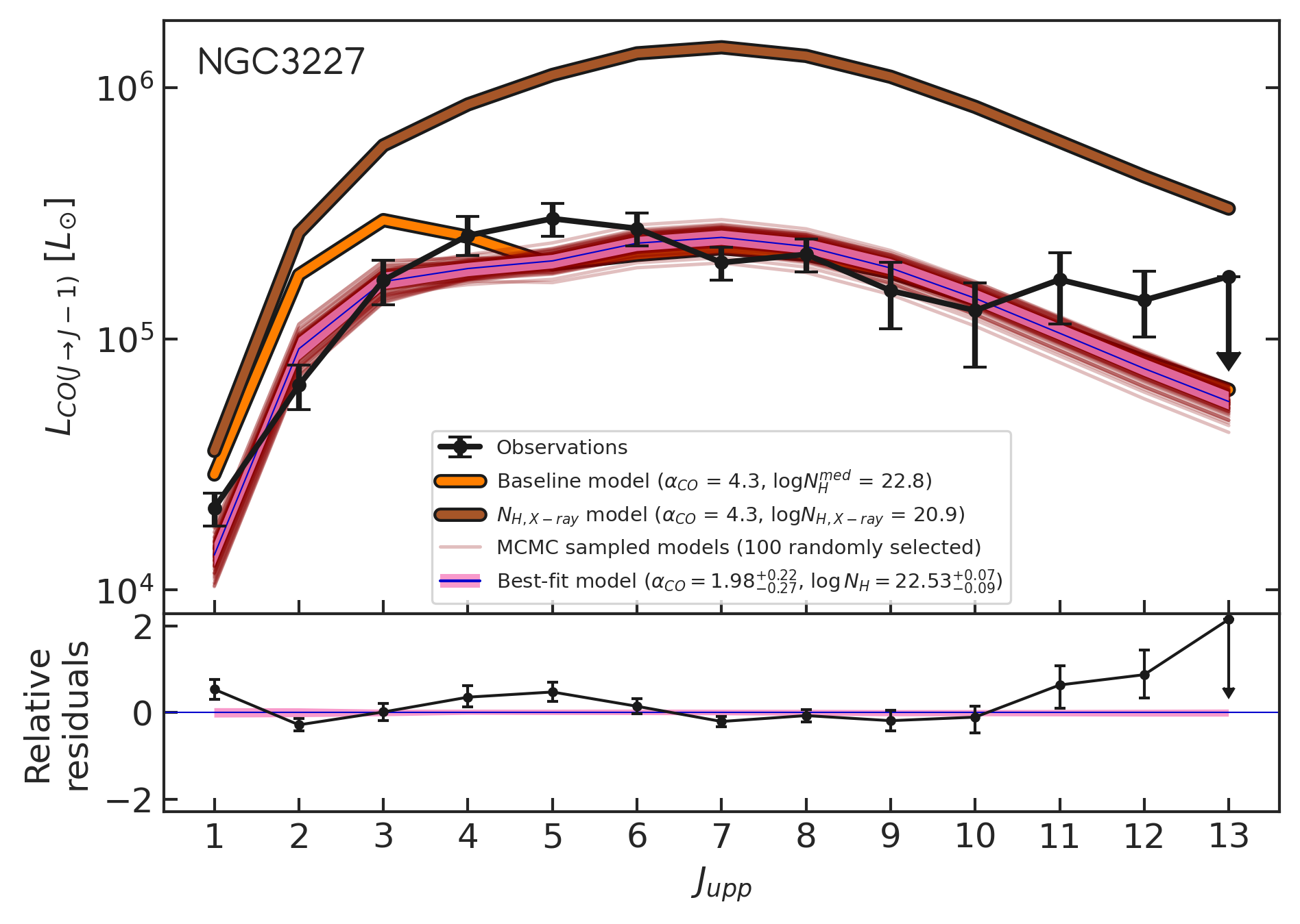
Figure 25: NGC 3227 CO SLEDs.

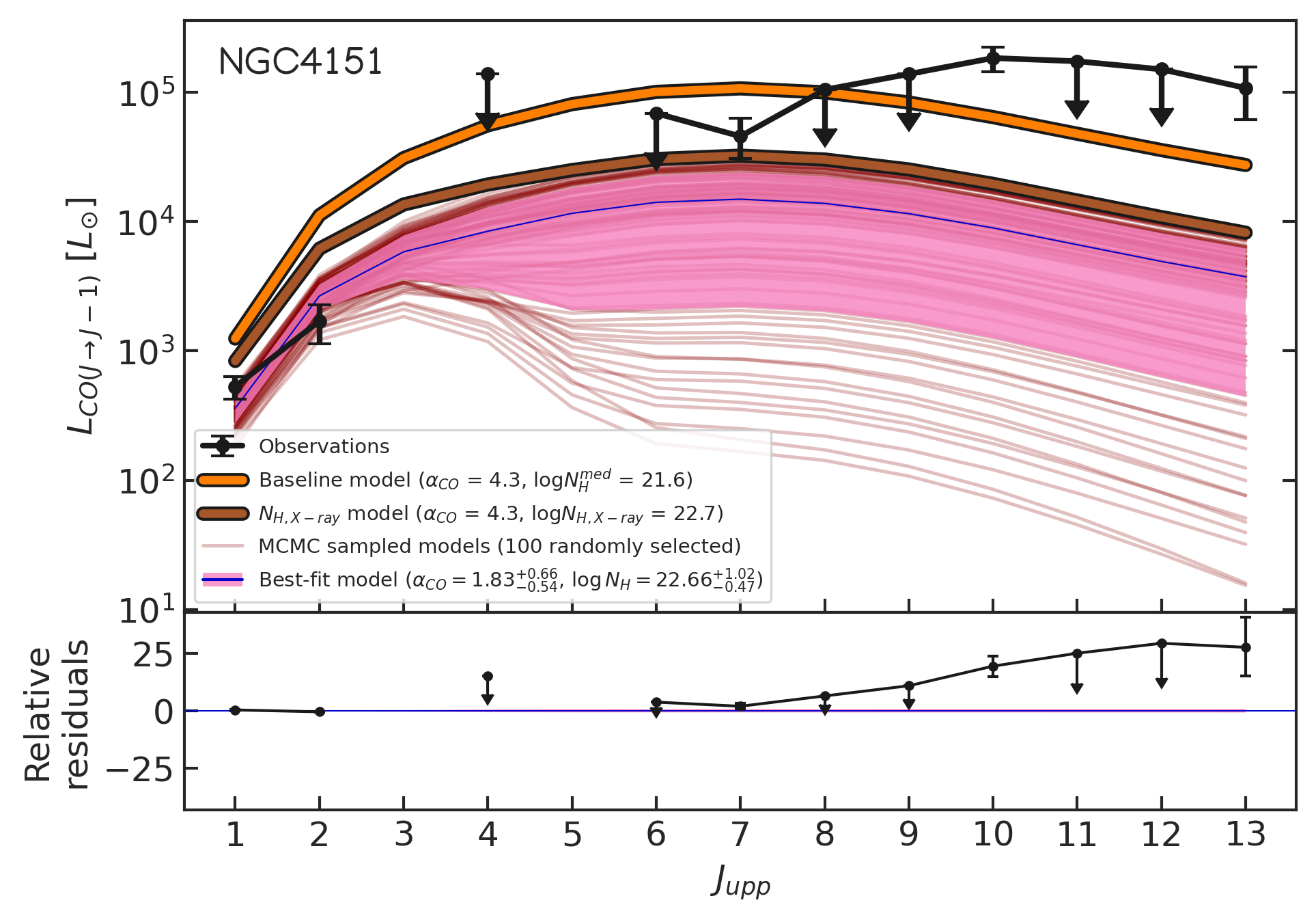
Figure 26: NGC 4151 CO SLEDs.

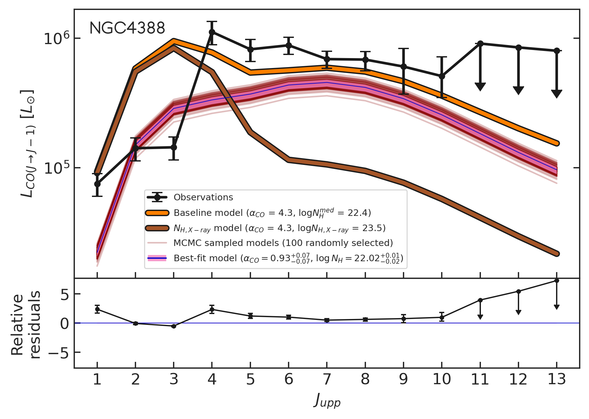
Figure 27: NGC 4388 CO SLEDs.

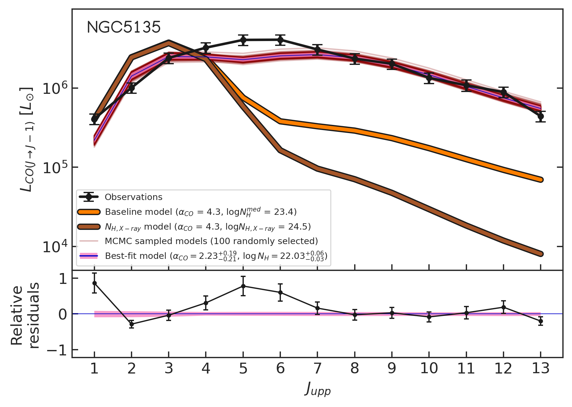
Figure 28: NGC 5135 CO SLEDs.

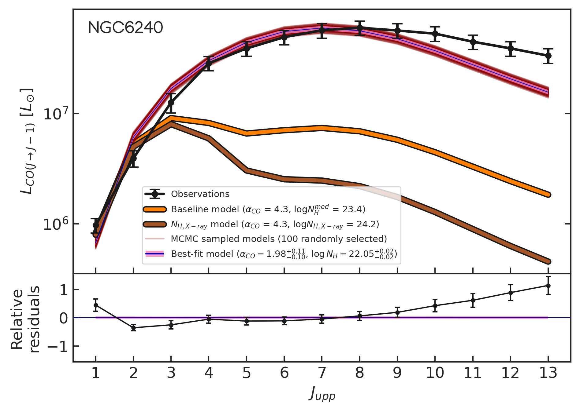
Figure 29: NGC 6240 CO SLEDs.

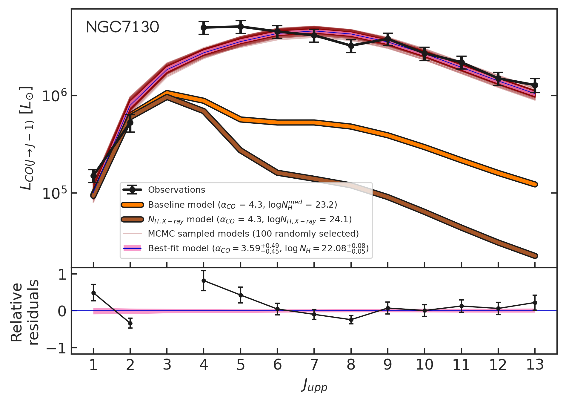
Figure 30: NGC 7130 CO SLEDs.

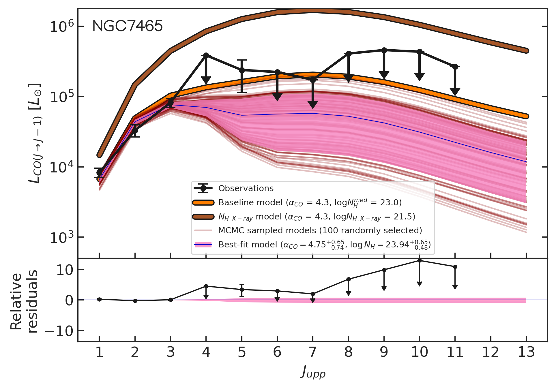
Figure 31: NGC 7465 CO SLEDs.

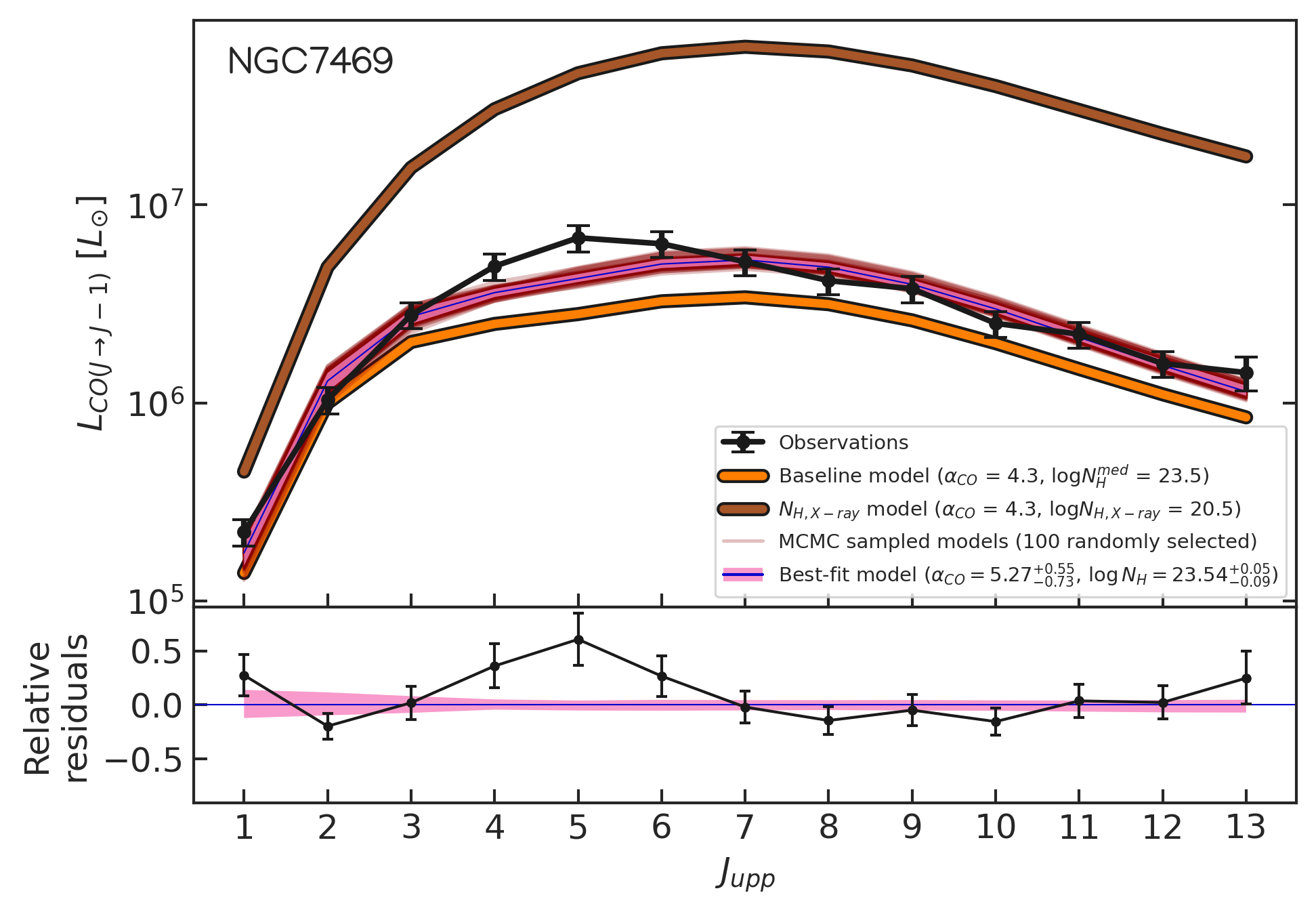
Figure 32: NGC 7469 CO SLEDs.

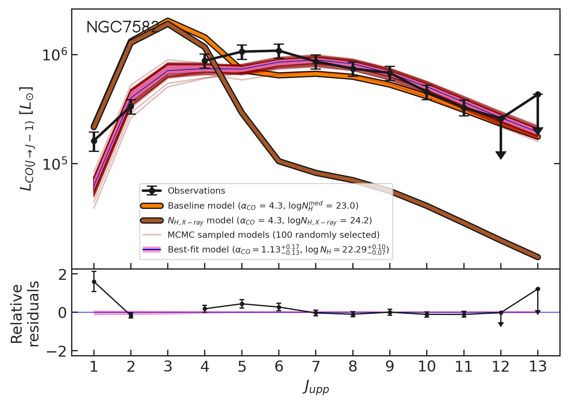
Figure 33: NGC 7582 CO SLEDs.

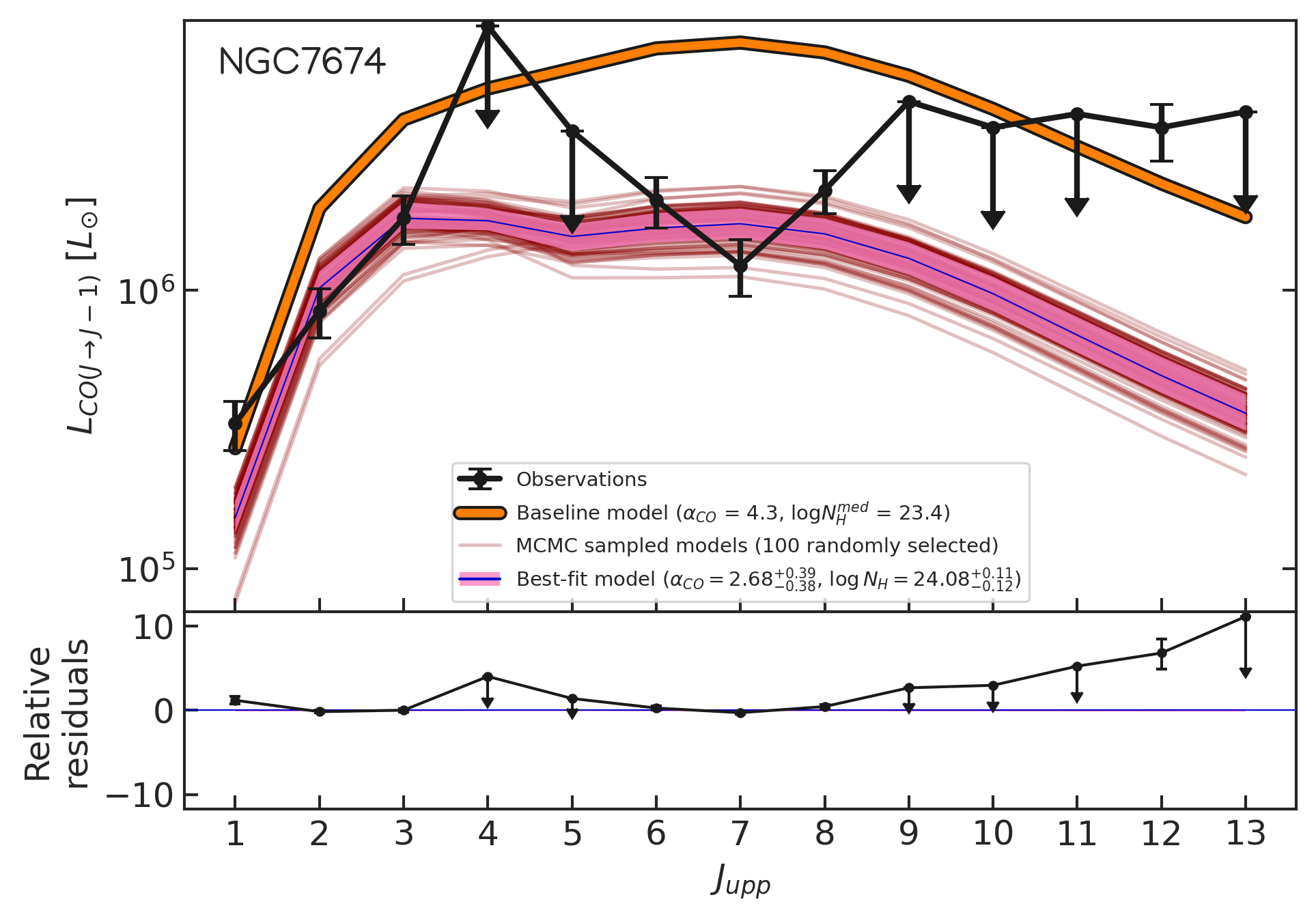
Figure 34: NGC 7674 (Mrk 533) CO SLEDs.

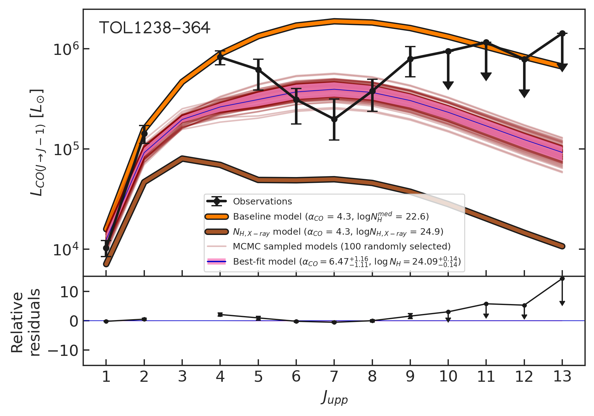
Figure 35: TOL 1238-364 (IC 3639) CO SLEDs.

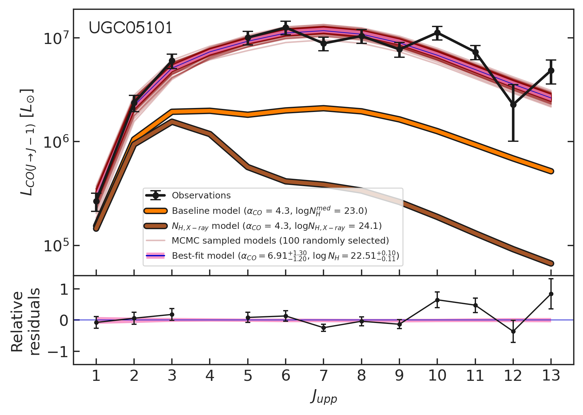
Figure 36: UGC 5101 CO SLEDs.

References

- Accurso et al. (2017) Accurso G., et al., 2017, MNRAS, 470, 4750
- Alonso-Herrero et al. (2012) Alonso-Herrero A., Pereira-Santaella M., Rieke G. H., Rigopoulou D., 2012, ApJ, 744, 2
- Alonso Herrero et al. (2023) Alonso Herrero A., et al., 2023, A&A, 675, A88
- Astropy Collaboration et al. (2013) Astropy Collaboration et al., 2013, A&A, 558, A33
- Astropy Collaboration et al. (2018) Astropy Collaboration et al., 2018, AJ, 156, 123
- Ballesteros-Paredes et al. (2020) Ballesteros-Paredes J., et al., 2020, Space Sci. Rev., 216, 76
- Bellocchi et al. (2020) Bellocchi E., et al., 2020, A&A, 642, A166
- Bisbas et al. (2023) Bisbas T. G., van Dishoeck E. F., Hu C.-Y., Schruba A., 2023, MNRAS, 519, 729
- Bolatto et al. (2013) Bolatto A. D., Wolfire M., Leroy A. K., 2013, ARA&A, 51, 207
- Boquien et al. (2019) Boquien M., Burgarella D., Roehlly Y., Buat V., Ciesla L., Corre D., Inoue A. K., Salas H., 2019, A&A, 622, A103
- Boselli et al. (2014) Boselli A., Cortese L., Boquien M., 2014, A&A, 564, A65
- Bradford et al. (2009) Bradford C. M., et al., 2009, ApJ, 705, 112
- Brightman & Nandra (2011) Brightman M., Nandra K., 2011, MNRAS, 413, 1206
- Brunetti et al. (2021) Brunetti N., Wilson C. D., Sliwa K., Schinnerer E., Aalto S., Peck A. B., 2021, MNRAS, 500, 4730
- Butterworth et al. (2022) Butterworth J., Holdship J., Viti S., García-Burillo S., 2022, A&A, 667, A131
- Calura et al. (2022) Calura F., et al., 2022, MNRAS, 516, 5914
- Carilli & Walter (2013) Carilli C. L., Walter F., 2013, ARA&A, 51, 105
- Casasola et al. (2017) Casasola V., et al., 2017, A&A, 605, A18
- Casasola et al. (2020) Casasola V., et al., 2020, A&A, 633, A100
- Casasola et al. (2022) Casasola V., et al., 2022, A&A, 668, A130
- Cattaneo (2019) Cattaneo A., 2019, Nature Astronomy, 3, 896
- Chevance et al. (2023) Chevance M., Krumholz M. R., McLeod A. F., Ostriker E. C., Rosolowsky E. W., Sternberg A., 2023, in Inutsuka S., Aikawa Y., Muto T., Tomida K., Tamura M., eds, Astronomical Society of the Pacific Conference Series Vol. 534, Protostars and Planets VII. p. 1 (arXiv:2203.09570), doi:10.48550/arXiv.2203.09570
- Cicone et al. (2018) Cicone C., et al., 2018, ApJ, 863, 143
- Colombo et al. (2014) Colombo D., et al., 2014, ApJ, 784, 3
- Combes et al. (2013) Combes F., et al., 2013, A&A, 558, A124
- Davies et al. (2004) Davies R. I., Tacconi L. J., Genzel R., 2004, ApJ, 602, 148
- Domínguez-Fernández et al. (2020) Domínguez-Fernández A. J., et al., 2020, A&A, 643, A127
- Dunne et al. (2022) Dunne L., Maddox S. J., Papadopoulos P. P., Ivison R. J., Gomez H. L., 2022, MNRAS, 517, 962
- Dutkowska & Kristensen (2022) Dutkowska K. M., Kristensen L. E., 2022, A&A, 667, A135
- Eibensteiner et al. (2022) Eibensteiner C., et al., 2022, A&A, 659, A173
- Elia et al. (2021) Elia D., et al., 2021, MNRAS, 504, 2742
- Ellison et al. (2019) Ellison S. L., Viswanathan A., Patton D. R., Bottrell C., McConnachie A. W., Gwyn S., Cuillandre J.-C., 2019, MNRAS, 487, 2491
- Ellison et al. (2021) Ellison S. L., Lin L., Thorp M. D., Pan H.-A., Scudder J. M., Sánchez S. F., Bluck A. F. L., Maiolino R., 2021, MNRAS, 501, 4777
- Elmegreen & Scalo (2004) Elmegreen B. G., Scalo J., 2004, ARA&A, 42, 211
- Esparza-Arredondo et al. (2021) Esparza-Arredondo D., Gonzalez-Martín O., Dultzin D., Masegosa J., Ramos-Almeida C., García-Bernete I., Fritz J., Osorio-Clavijo N., 2021, A&A, 651, A91
- Esposito et al. (2022) Esposito F., Vallini L., Pozzi F., Casasola V., Mingozzi M., Vignali C., Gruppioni C., Salvestrini F., 2022, MNRAS, 512, 686
- Fabian (2012) Fabian A. C., 2012, ARA&A, 50, 455
- Farrah et al. (2022a) Farrah D., et al., 2022a, Universe, 9, 3
- Farrah et al. (2022b) Farrah D., et al., 2022b, MNRAS, 513, 4770
- Federrath & Klessen (2013) Federrath C., Klessen R. S., 2013, ApJ, 763, 51
- Federrath et al. (2008) Federrath C., Klessen R. S., Schmidt W., 2008, ApJ, 688, L79
- Federrath et al. (2011) Federrath C., Sur S., Schleicher D. R. G., Banerjee R., Klessen R. S., 2011, ApJ, 731, 62
- Fei et al. (2023) Fei Q., Wang R., Molina J., Shangguan J., Ho L. C., Bauer F. E., Treister E., 2023, ApJ, 946, 45
- Ferland et al. (2017) Ferland G. J., et al., 2017, Rev. Mex. Astron. Astrofis., 53, 385
- Fiore et al. (2017) Fiore F., et al., 2017, A&A, 601, A143
- Foreman-Mackey (2016) Foreman-Mackey D., 2016, The Journal of Open Source Software, 1, 24
- Foreman-Mackey et al. (2013) Foreman-Mackey D., Hogg D. W., Lang D., Goodman J., 2013, PASP, 125, 306
- Fukui & Kawamura (2010) Fukui Y., Kawamura A., 2010, ARA&A, 48, 547
- Galliano et al. (2003) Galliano E., Alloin D., Granato G. L., Villar-Martín M., 2003, A&A, 412, 615
- García-Bernete et al. (2021) García-Bernete I., et al., 2021, A&A, 645, A21
- García-Burillo et al. (2014) García-Burillo S., et al., 2014, A&A, 567, A125
- García-Burillo et al. (2019) García-Burillo S., et al., 2019, A&A, 632, A61