Braids and Higher-order Exceptional Points from the Interplay Between Lossy Defects and Topological Boundary States

Abstract

We show that the perturbation of the Su-Schrieffer-Heeger chain by a localized lossy defect leads to higher-order exceptional points (HOEPs). Depending on the location of the defect, third- and fourth- order exceptional points (EP3s & EP4s) appear in the space of Hamiltonian parameters. On the one hand, they arise due to the non-Abelian braiding properties of exceptional lines (ELs) in parameter space. Namely, the HOEPs lie at intersections of mutually non-commuting ELs. On the other hand, we show that such special intersections happen due to the fact that the delocalization of edge states, induced by the non-Hermitian defect, hybridizes them with defect states. These can then coalesce together into an EP3. When the defect lies at the midpoint of the chain, a special symmetry of the full spectrum can lead to an EP4. In this way, our model illustrates the emergence of interesting non-Abelian topological properties in the multiband structure of non-Hermitian perturbations of topological phases.

Non-Hermitian systems are known to display exceptional points (EP), unconventional spectral singularities where the Hamiltonian becomes defective due to the coalescence of eigenstates Heiss (2012, 2004); Berry (2004); Yuto Ashida and Ueda (2020); Bergholtz et al. (2021). These have been observed in various experimental platforms such as electronic circuits Stehmann et al. (2004), microwave cavities Dembowski et al. (2001), acoustics Shi et al. (2016) and photonics Özdemir et al. (2019); Miri and Alu (2019), and recently were shown to enhance superconductivity Arouca et al. (2023), speed up entanglement generation Li et al. (2023a) and enhance quantum heat engines Bu et al. (2023). In addition to the famously anomalous bulk-boundary correspondence of non-Hermitian systems Yao and Wang (2018); Lee (2016); Xiong (2018); Kunst et al. (2018); Xiao et al. (2020); Helbig et al. (2020); Ghatak et al. (2020); Borgnia et al. (2020); Li et al. (2021); Okuma and Sato (2023), non-Hermitian defects in topological (Hermitian or non-Hermitian) systems also lead to new phenomena, such as the emergence of EPs Jana and Sirota (2023); Tzortzakakis et al. (2022), the amplification of topological defect states Schomerus (2013); Poli et al. (2015), and anomalous skin effects Guo et al. (2023a); Li et al. (2023b); Molignini et al. (2023). In this Letter, we report on qualitatively different consequences of the interplay between Hermitian band topology and non-Hermitian (lossy) defects that manifest only in multi-band systems, namely, through the non-Abelian topology of EPs.

Figure 1: (a) Schematic diagram of the Su-Sherieffer-Heeger chain with a lossy defect. (b) Formation of PEP2s, an EP3 and an EP4 from the merging of EPs. From the braiding of eigenvalues (right) as one traces a loop around an EP (left), one sees that these three different cases arise from the different numbers of common states between the braidings on each merging EP.

In multi-band systems, higher-order exceptional points (HOEP) can appear, where $N>2$ states simultaneously coalesce, also known as $N$-th order exceptional points (EP$N$). Symmetry and topology play a major role in classifying and protecting EPs Ding et al. (2022); Patil et al. (2022); Delplace et al. (2021); Mandal and Bergholtz (2021); Carlström et al. (2019); Zhang et al. (2021); Hu and Zhao (2021); Zhong et al. (2018); Hu et al. (2022); Rui et al. (2019); Luitz and Piazza (2019); Zhou et al. (2018); Guo et al. (2023b); König et al. (2023); Wojcik et al. (2022); Lin et al. (2019); González and Molina (2017); Ryu et al. (2012); Kozii and Fu (2017); Hu et al. (2023); Yang et al. (2023); Budich et al. (2019); Kawabata et al. (2019); Kimura et al. (2019); Okugawa and Yokoyama (2019); Szameit et al. (2011); Yoshida et al. (2019); Yang and Mandal (2023); Zhou et al. (2019); Stålhammar and Bergholtz (2021); Crippa et al. (2021); Wang et al. (2023), with the topological invariant associated to an EP being the eigenvalue braiding on an encircling loop in the space of Hamiltonian parameters. It corresponds to an element of the non-Abelian braid group Wojcik et al. (2020); Li and Mong (2021); Delplace et al. (2021); Kawabata et al. (2019), and in particular the formation of HOEPs can be accounted for in terms of the merging of non-commuting EP2s. We show that this structure naturally appears in the spectrum of the Su-Schrieffer-Heeger (SSH) chain perturbed by a localized lossy defect, and a rich landscape of exceptional degeneracies appears in the 3D parameter space formed by the (real) SSH gap $\Delta$ and the (complex) defect strength $\gamma$ (figure 1(a)). If the defect is located at: the edge site, a generic bulk site, or the mid-point of the chain, then we find that: paired EP2s (PEP2s) where EP2s connecting different states appear at the same point, an EP3, or an EP4, respectively, appear. We classify them in terms of the non-Abelian merging of EP2s with different braid invariants, as schematically represented in figure 1(b). One finds that the HOEPs only appear in the topological sector of parameter space $\Delta>0$. We explain this fact by studying the effect of the defect on the topological edge states. We find that, in the multiband context, the previously noted delocalization of edge states can lead to their coalescence with defect states, which in parameter space translates into the merging of non-commuting EPs into a HOEP. This reveals a new way in which the topology of non-Hermitian systems is correlated with the topology of their Hermitian counterparts.

The model — We consider a perturbation of the SSH chain by a single lossy defect at odd site $2s-1$,

$$H=H_{0}-i\gamma|2s-1\rangle\langle 2s-1|,$$ (1)

where

$$H_{0}=-\sum_{j=1}^{2N-1}(t+(-1)^{j}\Delta)|j\rangle\langle j+1|+\text{h.c.}$$ (2)

is the SSH Hamiltonian on a chain of length $2N$, and we investigate the non-dimerized regime $|\Delta|<1$. Note that one can recover the case of a defect at an even site by reversing the chain. Also, since the spectrum is symmetric with respect of the sign of $\gamma$, we focus on the dissipative regime $\text{Re}(\gamma)>0$. In our notations, the hopping strength is normalized to $t=1$. The topologically nontrivial phase corresponds to $\Delta>0$, for which the spectrum of (2) contains edge states protected by chiral symmetry Heeger et al. (1988). As we will see, the structure of non-Hermitian degeneracies is also different in this phase.

Exceptional lines and higher-order degeneracies — Degeneracies in the spectrum of Hamiltonian $H$ correspond to repeated roots of the characteristic polynomial

$$p(\lambda;\mathbf{R})\equiv\det(H(\mathbf{R})-\lambda I),$$ (3)

whose variable is $\lambda$ and coefficients depend on the Hamiltonian parameters $\mathbf{R}$. The condition for the existence of a $k$-th order degeneracy is the vanishing of the resultants between $p(\lambda;\mathbf{R})$ and its first $k-1$ derivatives in $\lambda$ Janson (2007); Woody (2016), which leads to $k-1$ polynomial equations on the parameters $\mathbf{R}$. Since the resultants are complex expressions, one in general needs to tune $2(k-1)$ real parameters to locate a $k$-th order degeneracy Mandal and Bergholtz (2021); Delplace et al. (2021); Sayyad and Kunst (2022).

Figure 2: Exceptional lines (top) and eigenvalue braidings (bottom). (a)-(c): ELs which merge into PEP2 and HOEPs, for different defect locations. The dashed lines are the predictions for $\gamma_{\rm edge}(\Delta)$, $\gamma_{\rm defect}(\Delta)$, and $\gamma_{\rm mixed}(\Delta)$. The inset shows all the ELs in the larger range of $\Delta\in[-1,1]$. (a): When $s=1$ (edge defect), PEP2s are formed. (b): When $s=2$ (bulk defect), an EP3 is formed. (c): When $s=3$ (midpoint defect), an EP4 is formed. (d)-(f): Braiding eigenvalues on a loop ($\theta\in[0,2\pi)$) encircling the intersection of ELs. For different ELs, the path is chosen as (d) $\gamma=1.25+0.2ie^{i\theta}$, $\Delta=-0.2$. (e) $\gamma=2.83+0.2ie^{i\theta}$, $\Delta=0.48$. (f) $\gamma=2.28+0.2ie^{i\theta}$, $\Delta=0.14$. For all figures, $2N=8$.

Remarkably, we obtained the analytical expression of the characteristic polynomial of the Hamiltonian (1) sup :

$$p(\lambda;\Delta,\gamma)=(1-\Delta^{2})^{N}\times$$ (4)

$$\left[(U_{N}+rU_{N-1})+\frac{i\gamma\lambda}{1-\Delta^{2}}(U_{s-1}+rU_{s-2})U_{N-s}\right],$$

where $r=\frac{1+\Delta}{1-\Delta}$, $U_{n}=U_{n}(Q)$ is the $n$-th Chebyshev polynomial of the second kindMason and Handscomb (2002), and $Q=\frac{\lambda^{2}-2(1+\Delta^{2})}{2(1-\Delta^{2})}$.

We solve for degeneracies by computing the corresponding resultants in the 3D parameter space $(\Delta,{\rm Re}(\gamma),{\rm Im}(\gamma))$. The condition for a two-fold degeneracy is given by the vanishing of a single resultant, which leads to two real equations. Thus the potential EP2s extend into exceptional lines (EL), which we plot in figures 2(a)-2(c) for a chain of length $2N=8$. Degeneracies of higher multiplicity can appear at the intersections of ELs, and we find that they are qualitatively different depending on whether the defect lies at the boundary, at the mid-point of the chain, or at a generic bulk site.

Non-Abelian braidings characterizing EPs — Exceptional degeneracies can be distinguished from normal degeneracies through the braiding of eigenvalues on a loop enclosing the EP in parameter space Hu et al. (2022). The most well-explored example is the coalescence of two eigenvectors at a square-root branch point of the eigenvalues Dykhne (1960); Hwang and Pechukas (1977); Wang et al. (2022); Cardoso (2023). The generalization is the braiding of $N$ eigenvalues on a loop enclosing the EP$N$, where the $N$ corresponding eigenvectors coalesce.

The braiding group element on a given loop can be computed by defining a reference ordering of the eigenvalues (such as in terms of their real parts) and taking the crossing of the $i$-th eigenvalue over (respectively, under) the $i+1$-th eigenvalue to correspond to $\sigma_{i}$ (resp., $\sigma_{i}^{-1}$). The braid group is generated by the $\sigma_{i}$ with the rules Fox and Neuwirth (1962)

$$\sigma_{i}\sigma_{i+1}\sigma_{i}=\sigma_{i+1}\sigma_{i}\sigma_{i+1},\quad\sigma_{i}\sigma_{j}=\sigma_{j}\sigma_{i}\ (|j-i|>1).$$ (5)

Under continuous deformations of the loop which do not cross any additional EPs, the braiding only changes by a Markov move Birman (1974), which corresponds to a conjugation of the braid group element $b_{\rm loop}\mapsto gb_{\rm loop}g^{-1}$. Thus the conjugacy classes $[b_{\rm loop}]$ are topological invariants of the EPs, and get multiplied when EPs merge Guo et al. (2023b).

In three dimensions, the EP2s extend into ELs, and the braid invariants are computed from loops enclosing the ELs. They satisfy a non-Abelian conservation rule (NACR): invariants $[b]$ are constant as the loop moves along each isolated EL, and get multiplied when other ELs enter/leave the loop. In particular, if two ELs intersect forming a HOEP, then one can infer that there is a common state among the ones braiding around each EL. From equation (5), we see that the corresponding braid invariants do not commute. Conversely, if the braid invariants of the intersecting ELs do commute, then one can infer that the states braiding around each EL form two distinct pairs, and a HOEP is not formed. Instead, one has PEP2s. Both cases are schematically illustrated in figure 1(b), and we find that both happen in the defect SSH chain (1).

When the defect is located at the edge $s=1$, two ELs (magenta and light blue) intersect forming PEP2s, as shown in figure 2(a). Indeed, the braid invariants corresponding to the intersecting ELs commute, and any path enclosing both lines has braiding $[b_{\rm PEP2}]=[\sigma_{3}\sigma_{5}]$ (figure 2(d)).

When the defect is located at a generic bulk site, an EP3 appears. It lies at the intersection of the orange and yellow lines in figure 2(b), and the braiding on a loop enclosing the intersection, $\sigma_{4}^{-1}\sigma_{3}\sigma_{4}\sigma_{5}$, is shown in figure 2(e). To see that this product corresponds to a triple braiding of the eigenvalues, we bring it to standard form by a Markov move,

$$(\sigma_{5}\sigma_{4})(\sigma_{4}^{-1}\sigma_{3}\sigma_{4}\sigma_{5})(\sigma_{5}\sigma_{4})^{-1}=\sigma_{3}\sigma_{4},$$ (6)

where we used that $\sigma_{5}\sigma_{4}\sigma_{5}=\sigma_{4}\sigma_{5}\sigma_{4}$. Thus $[b_{\rm EP3}]=[\sigma_{3}\sigma_{4}]$, with the product of non-commuting braids capturing the triple braiding of eigenvalues characteristic of an EP3.

To understand how the NACR applies to the merging of non-commuting ELs into an EP3, let us consider the braid invariant $[b]$ evaluated on a loop enclosing both the orange and the yellow lines at fixed values of $\Delta$. We find that at $\Delta_{i}=-0.9$, $[b_{i}]=[\sigma_{3}\sigma_{5}]$, corresponding to the braiding of two separate pairs of eigenvalues as in the PEP2s case above. Thus at this value of $\Delta$ the ELs commute, with braid invariants $[\sigma_{3}]$ and $[\sigma_{5}]$. As one tunes $\Delta$ up to its value at the intersection $\Delta_{f}\approx 0.5$, the enclosing loop intersects with a third EL twice (blue curve in figure 2(b)). This EL has braiding $[\sigma_{4}]$, which does not commute with either of the ELs and in fact entangles the braidings $[\sigma_{3}]$ and $[\sigma_{5}]$. Since the blue EL comes in and out of the loop as one tunes $\Delta$, we again find that $[b_{f}]=[\sigma_{4}^{-1}\sigma_{3}\sigma_{4}\sigma_{5}]$. By equation (6), $[b_{f}]=[\sigma_{3}\sigma_{4}]$, so that an EP3 appears and the merging ELs do not commute at $\Delta_{f}$. Thus in this example, the initially commuting ELs ends up non-commuting, resulting in HOEPs, due to their non-Abelian braiding with other ELs in parameter space Ding et al. (2016); Doppler et al. (2016).

A special case appears when the sublattice length $N$ is even and the defect location $2s-1$ corresponds to the mid-point, $s=\frac{N}{2}+1$. At the intersection of the green and yellow curves in figure 2(c) we find an EP4, with braiding $[b_{\rm EP4}]=[\sigma_{1}(\sigma_{3}\sigma_{4}\sigma_{5})\sigma_{7}]$ (see figure 2(f)). That this only happens when the sublattice length $N$ is even reveals a new instance of the even-odd effects characteristic of non-Hermitian systems Joglekar et al. (2010); Burke et al. (2020). Another interesting aspect of this result is that typically one only expects an EP4 to appear at the intersection of at least three non-commuting EP2s. Here, the EP4 appears because the green line is a very special case, which we call a stable PEP2. Along the whole green line, the whole spectrum coalesces in pairs. Indeed, we find that this line is exactly given by $\gamma=2(1+\Delta)$, and that in this case the characteristic polynomial is a perfect square $p(\lambda)=q(\lambda)^{2}$ sup . A similar PEP2 was reported in Burke et al. (2020), which can be seen as a special case of the SSH chain when $\Delta=0$. Thus the invariant on the green line is $[\sigma_{1}\sigma_{3}\sigma_{5}\sigma_{7}]$, and its merging with the non-commuting yellow line $[\sigma_{4}]$ leads to the EP4 braiding $b_{\rm EP4}=[\sigma_{1}(\sigma_{3}\sigma_{4}\sigma_{5})\sigma_{7}]$, with the additional braiding of two separate pairs of levels, $[\sigma_{1}]$ and $[\sigma_{7}]$.

In the dimerized limits $\Delta=\pm 1$, the ELs converge to several fixed points. One fixed point is the Hermitian degeneracy at $\gamma=0$, where the EPs of opposite chirality, or equivalently with a braid invariant and its inverse, annihilate Król et al. (2022). In the bulk defect case, the ELs also converge at the EP of the dimerized chain $\gamma=4$. In the boundary defect case, a special fixed point appears at $\Delta=1$, $\gamma=\pm 2i$, where the boundary site becomes isolated. Interestingly, not all ELs are symmetric under sign change of $\Delta$. In fact, the HOEPs only appear in the topological phase $\Delta>0$. As we now discuss, the formation of HOEPs can be traced back to the topological edge state.

Figure 3: Delocalization of the edge states and defect states near $\gamma_{\rm mixed}\approx 2.82$. (a) Wavefunction profile of left edge states. (b) Wavefunction profile of defect state. In both figures, $2N=16,s=3,\Delta=0.3$.

The role of edge states — In the topological phase $\Delta>0$, the spectrum is gapped and to leading order one can study the effect of the non-Hermitian defect on the in-gap states separately. The projection of $H$ onto the edge states gives

$$H_{\rm eff}=\left(\begin{array}[]{cc}\langle L|H|L\rangle&\langle L|H|R\rangle\\ \langle R|H|L\rangle&\langle R|H|R\rangle\end{array}\right)\equiv\left(\begin{array}[]{cc}\mathcal{E}_{L}&J\\ J^{*}&\mathcal{E}_{R}\end{array}\right).$$ (7)

The overlap $J\propto r^{-N}$ is responsible for the exponentially small energy splitting in the Hermitian case, $\mathcal{E}_{L}\propto i\gamma r^{-2s}$ is proportional to the squared amplitude of the edge state at the defect site $2s-1$, and $\mathcal{E}_{R}=0$ for our choice of placing the defect at an odd site. Here, $r^{-1}=\frac{1-\Delta}{1+\Delta}=e^{-\xi}$ parametrizes the decay length $\xi$ of the edge states. This two-level Hamiltonian has an exceptional point at $\mathcal{E}_{L}^{2}=4|J|^{2}$. In the dissipative region $\text{Re}(\gamma)>0$ this gives the exceptional point sup

$$\gamma_{\rm edge}=2(1+\Delta)r^{2s-2-N}.$$ (8)

The defect also leads to localized states in the bulk. In terms of the sublattice position index $l$, their wavefunctions are given by

$$\psi_{n}=\left\{\begin{aligned} &A\exp(-\kappa|l-s|),\hskip 28.45274ptn=2l\\ &B\exp(-\kappa|l-s+1|),\hskip 11.38092ptn=2l+1\end{aligned}\right.,$$ (9)

where the localization length $\kappa^{-1}$ and the corresponding eigenenergies $\lambda$ are given by

$$\lambda^{2}=2(1-\Delta^{2})\cosh(2\kappa)+2(1+\Delta^{2}),$$ (10)

$$\cosh(2\kappa)=\frac{-\gamma^{2}\pm\sqrt{(\gamma^{2}-4(1-\Delta)^{2})(\gamma^{2}-4(1+\Delta)^{2})}}{4(1-\Delta^{2})},$$

which have degeneracies $\gamma_{\pm}=2(1\pm\Delta)$ in the dissipative regime. The condition for localized states $\text{Re}(\kappa)>0$ singles out the exceptional point

$$\gamma_{\rm defect}=2(1+\Delta),$$ (11)

where the two defect states coalesce. A third possibility is the coalescence of one of the defect states with one of the edge states. When $\gamma\geq\max({\gamma_{\rm edge},\gamma_{\rm defect}}),$ the four eigenenergies become fully imaginary, and one can estimate that such a mixed coalescence happens at sup

$$\gamma_{\rm mixed}=(1+\Delta)r^{s-1}\sqrt{1-r^{-2N}}.$$ (12)

The coalescing wavefunctions in this case are shown in figures 3(a), 3(b).

Equations (8), (11), (12) approximate the ELs involving localized in-gap states, and are plotted as dashed lines in figures 2(a)-2(c). HOEPs can appear when they intersect at the saturation of the $\gamma_{\rm mixed}\geq\text{max}(\gamma_{\rm edge},\gamma_{\rm defect})$ bound. For $s<\frac{N}{2}+1$, $\gamma_{\rm defect}(\Delta)>\gamma_{\rm edge}(\Delta)$, and an EP3 appears at $\gamma_{\rm mixed}(\Delta_{\rm EP3})=\gamma_{\rm defect}(\Delta_{\rm EP3})$, whose solution $(\gamma_{\rm EP3},\Delta_{\rm EP3})$ is shown in figure 2(b) and is very close to the numerical value of the observed EP3. It corresponds to the simultaneous coalescence of the two defect states and the left edge state. For $s>\frac{N}{2}+1$, $\gamma_{\rm edge}(\Delta)>\gamma_{\rm defect}(\Delta)$, and an EP3 appears due to the simultaneous coalescence of the two edge states and one defect state at $\gamma_{\rm mixed}(\Delta_{\rm EP3})=\gamma_{\rm edge}(\Delta_{\rm EP3})$. Note that this asymmetry is due to our choice of placing the defect at an odd site $2s-1$. Instead, if the defect is located at $2s$, then the situation is reversed and, for $s>\frac{N}{2}+1$, an EP3 is formed due to the simultaneous coalescence of the two defect states and the right edge state.

When $N$ is even, there is a special case at the midpoint $s=\frac{N}{2}+1$, for which $\gamma_{\rm edge}(\Delta)=\gamma_{\rm defect}(\Delta)$, the stable PEP2. The four localized states coalesce, generating an EP4, at $\gamma_{\rm mixed}(\Delta_{\rm EP4})=\gamma_{\rm defect}(\Delta_{\rm EP4})=\gamma_{\rm edge}(\Delta_{\rm EP4})$. The solution is once again close to the numerically computed value, as shown in figure 2(c).

Finally, when $s=1$, no additional localized states are generated besides the edge states. Thus we only have $\gamma_{\rm edge}(\Delta)$, shown in figure 2(a), and no HOEP, but instead PEP2s formed from the coalescence of two pairs of scattering states.

In the thermodynamic limit $N\to\infty$, the exceptional degeneracy of the edge states $\gamma_{\rm edge}\to 0$ disappears into their exact Hermitian degeneracy. However, $\gamma_{\rm mixed}$ remains finite in the limit of a half-infinite chain where the distance of the defect to the boundary, $2s-1$, is kept fixed. Thus in this case the EP3 survives the thermodynamic limit and can be detected at finite loss rate $\gamma_{\rm EP3}$. It is worth emphasizing that this phenomenology is distinct from the anomalous bulk-boundary correspondence of fully non-Hermitian SSH models Yao and Wang (2018); Lee (2016); Xiong (2018); Kunst et al. (2018) at which the boundary modes form an EP2 in the thermodynamic limit Kunst et al. (2018) due to the non-Hermitian skin effect Okuma and Sato (2023); Lin et al. (2023).

Discussion – Recall that, from our counting of resultants, a degeneracy of multiplicity $3$ typically requires tuning $2(3-1)=4$ real parameters, and a degeneracy of multiplicity $4$ requires tuning $2(4-1)=6$ real parameters. However, we found that in the simple model of the SSH chain perturbed by a localized lossy defect, both an EP3 and an EP4 appear in the 3D space $(\Delta,{\rm Re}(\gamma),{\rm Im}(\gamma))$. The reason why this happens is two-fold. First, the SSH chain has topological edge states. While it was previously realized that non-Hermiticity can have the independent effects of (a) delocalizing the edge states Cheng et al. (2022); Zhu et al. (2021) and (b) leading to EPs due to the coalescence of non-Hermitian defect states Burke et al. (2020), we find that in fact (a) and (b) can collaborate to create HOEPs in our model by the simultaneous coalescence of two defect states and one edge state. This point is enough to explain the EP3. Second, when the chain length $2N$ is a multiple of $4$, ie. $N$ is even, and the defect is located at the midpoint $s=\frac{N}{2}+1$, stable PEP2s appear: a special EL where the full spectrum coalesces in pairs. Together with the first point, it leads to the simultaneous coalescence of the two defect states and the two edge states, forming the EP4. These two points reveal topological features of the model which only become apparent in the multiband non-Hermitian setting. In parameter space, they translate into the special intersections of non-commuting ELs, which manifest their non-Abelian braiding properties. Thus our example opens up a new window of exploration: what types of non-Abelian, non-Hermitian topology can arise from the interplay between local defects and boundary states in different symmetry classes? This question naturally branches out in two sets of intriguing problems: first, for the case of (symmetry-protected) Hermitian topological phases Hasan and Kane (2010); Qi and Zhang (2011); Chiu et al. (2016); Asbóth et al. (2016) with non-Hermitian defects as studied here in a minimal model and, second, non-Hermitian symmetry-protected phases which already in the bulk exhibit non-Abelian topological features Yang et al. (2023) which may be further enriched by the interplay between boundaries and defects.

Acknowledgments – This work was sponsored by Pujiang Talent Program 21PJ1405400, Jiaoda 2030 program WH510363001-1, and the Innovation Program for Quantum Science and Technology Grant No.2021ZD0301900. EJB is supported by the Swedish Research Council (VR, grant 2018-00313), the Wallenberg Academy Fellows program (2018.0460) of the Knut and Alice Wallenberg Foundation, and the Göran Gustafsson Foundation for Research in Natural Sciences and Medicine.

Supplementary Information

Appendix A I. General method to obtain degenerate points

Degeneracies correspond to multiple roots of the characteristic polynomial of the Hamiltonian, and can be found by computing the discriminant, which in turn can be obtained from the resultants. Explicitly, let us fix the notation for two monic polynomials $p(z)=a_{n}z^{n}+\cdots+a_{0}$ and $q(z)=b_{m}z^{m}+\cdots+b_{0}$. Their resultant is defined as

$${\rm Res}_{z}(p,q)=a_{n}^{m}\prod_{i=1}^{n}q(z_{i}),$$ (S1)

where $\{{z_{i}}\}$ is the full set of roots of the polynomial $p(z)$. Then the discriminant ${\rm Disc}_{z}(p)$ of the polynomial $p(z)$ can be obtained from the resultant of $p$ and $p^{\prime}$ as

$${\rm Disc}_{z}(p)=(-1)^{n(n-1)/2}a_{n}^{-1}{\rm Res}_{z}(p,p^{\prime}).$$ (S2)

A convenient result is that the resultant can be evaluated through the determinant of the Sylvester matrix $\mathcal{S}(p,q)$,

$${\rm Res}_{z}(p,q)={\rm det}\ {\mathcal{S}}(p,q),$$ (S3)

where $\mathcal{S}(p,q)$ is the $(m+n)\times(m+n)$ matrix

$$\mathcal{S}(p,q)=\left(\begin{matrix}a_{n}&a_{n-1}&a_{n-2}&\ldots&0&0&0\\ 0&a_{n}&a_{n-1}&\ldots&0&0&0\\ \vdots&\vdots&\vdots&&\vdots&\vdots&\vdots\\ 0&0&0&\ldots&a_{1}&a_{0}&0\\ 0&0&0&\ldots&a_{2}&a_{1}&a_{0}\\ b_{m}&b_{m-1}&b_{m-2}&\ldots&0&0&0\\ 0&b_{m}&b_{m-1}&\ldots&0&0&0\\ \vdots&\vdots&\vdots&&\vdots&\vdots&\vdots\\ 0&0&0&\ldots&b_{1}&b_{0}&0\\ 0&0&0&\ldots&b_{2}&b_{1}&b_{0}\\ \end{matrix}\right).$$ (S4)

For example, for quadratic polynomial $p=az^{2}+bz+c$, the determinant of the Sylvester matrix between $p$ and $p^{\prime}=2az+b$ is

$$\det\mathcal{S}(p,q)=\left|\begin{matrix}a&b&c\\ 2a&b&0\\ 0&2a&b\end{matrix}\right|=-a(b^{2}-4ac),$$ (S5)

which gives the usual formula for the discriminant ${\rm Disc}_{z}(p)=b^{2}-4ac$.

If a polynomial has a root $z^{*}$ with multiplicity $n$, its derivatives up to $n-1$ order must be zero at $z^{*}$,

$$p(z^{*})=p^{\prime}(z^{*})=\cdots=p^{(n)}(z^{*})=0,$$ (S6)

$$p^{(n+1)}(z^{*})\neq 0,$$ (S7)

where the last inequality guarantees that $z^{*}$ is not a root of multiplicity $n+1$. Since these mean that $z^{*}$ is a common root, one finds the conditions

$${\rm Res}_{z}\left(p,\frac{\partial^{l}p}{\partial z^{l}}\right)=0\quad(l=1,\cdots,n),$$ (S8)

$${\rm Res}_{z}\left(p,\frac{\partial^{n+1}p}{\partial z^{k+1}}\right)\neq 0,$$ (S9)

in terms of the coefficients of $p$.

For degenerate points with multiplicity $2$, one has a single complex equation for the vanishing resultant, or equivalently two real equations. In our setup, we consider the three-dimensional parameter spaced formed by the real and imaginary parts of the complex defect strength $\gamma$ and real SSH gap parameter $\Delta$. Thus for each fixed $\Delta$, the degeneracies are given by the solutions of a complex equation for $\gamma$. The roots can be found by several numerical methods, We turn now to the calculation of the characteristic polynomial.

Appendix B II. Characteristic polynomial

The characteristic matrix $\lambda I-H$ of the SSH Hamiltonian with lossy defect has a tridiagonal form,

$$\lambda I-H=\left(\begin{matrix}a_{1}&b_{1}&&&\\ c_{1}&a_{2}&b_{2}&&\\ &c_{2}&a_{3}&b_{3}&\\ &&&\ddots&b_{n-1}\\ &&&c_{n-1}&a_{n}\end{matrix}\right),$$ (S10)

with coefficients

$$b_{n}=c_{n}=\left\{\begin{aligned} &1-\Delta&n=2l-1,\,\forall l\\ &1+\Delta&n=2l,\,\forall l\end{aligned}\right.,\quad a_{n}=\left\{\begin{aligned} &\lambda&n\neq 2s-1\\ &\lambda+i\gamma\quad&n=2s-1\end{aligned}\right..$$ (S11)

The determinant $P_{n}$ of a tridiagonal matrix (S10) satisfies the recurrence relation

$$P_{n}=a_{n}P_{n-1}-b_{n-1}c_{n-1}P_{n-2},$$ (S12)

which can be proved using Laplace’s expansion theorem. In the absence of defect, this recurrence relation becomes

$$\left\{\begin{aligned} &P_{2l}=\lambda P_{2l-1}-(1-\Delta)^{2}P_{2l-2}\\ &P_{2l+1}=\lambda P_{2l}-(1+\Delta)^{2}P_{2l-1}\end{aligned}\right.,$$ (S13)

and it can be solved by the ansatz $P_{2l}=Az^{l},P_{2l+1}=Cz^{l}$. Substituting the ansatz in (S13) one finds two roots,

$$z_{\pm}=(1-\Delta^{2})(Q\pm\sqrt{Q^{2}-1}),$$ (S14)

where $Q=\frac{\lambda^{2}-2(1+\Delta^{2})}{2(1-\Delta^{2})}$. For simplicity, we define $z=Q+\sqrt{Q^{2}-1}=(Q-\sqrt{Q^{2}-1})^{-1}$, so that $P_{2l}=(1-\Delta^{2})^{l}(Az^{l}+Bz^{-l})$ and $P_{2l+1}=(1-\Delta^{2})^{l}(Cz^{l}+Dz^{-l})$ where, by (S13), only two of the $A,B,C,D$ coefficients are independent and should be determined by initial conditions. It is convenient, however, to treat them as independently determined by $P_{0}$, $P_{1}$, $P_{2}$ and $P_{3}$. We find

$$P_{2l}=(1-\Delta^{2})^{l-1}(P_{2}U_{l-1}-(1-\Delta^{2})P_{0}U_{l-2}),$$ (S15)

$$P_{2l+1}=(1-\Delta^{2})^{l-1}(P_{3}U_{l-1}-(1-\Delta^{2})P_{1}U_{l-2}).$$

Here, $U_{n}=U_{n}(Q)$ is the $n$-th Chebishev polynomial of the second kind, and in deriving this formula we used that $Q=\frac{z+z^{-1}}{2}$ and the property

$$U_{n}\left(\frac{z+z^{-1}}{2}\right)=\frac{z^{n+1}-z^{-n-1}}{z-z^{-1}}.$$ (S16)

Additional useful properties of Chebyshev polynomials are Mason and Handscomb (2002):

$$U_{n}(x)=2xU_{n-1}(x)-U_{n-2}(x),$$ (S17)

$$U_{n}=U_{m}U_{n-m}-U_{m-1}U_{n-m-1},$$

$$\frac{dU_{n}(x)}{dx}=\frac{(n+1)U_{n+1}-nxU_{n}}{1-x^{2}}.$$

For the unperturbed SSH chain, $P_{0}^{(0)}=1$, $P_{1}^{(0)}=\lambda$, $P_{2}^{(0)}=\lambda^{2}-(1-\Delta)^{2}$, $P_{3}^{(0)}=\lambda(\lambda^{2}-2(1+\Delta^{2}))$, so that (S15) gives

$$P_{2l}^{(0)}=(1-\Delta^{2})^{l}\left(U_{l}+rU_{l-1}\right),$$ (S18)

$$P_{2l+1}^{(0)}=(1-\Delta^{2})^{l}\lambda U_{l},$$

where $r=\frac{1+\Delta}{1-\Delta}$. Thus the characteristic polynomial of the SSH Hamiltonian with $2N$ sites is

$$P_{2N}^{(0)}=(1-\Delta^{2})^{N}\left(U_{N}+rU_{N-1}\right).$$ (S19)

The presence of a lossy defect at site $2s-1$ changes the recurrence at a single site, so that

$$P_{2s-1} =(\lambda+i\gamma)P_{2s-2}-(1+\Delta)^{2}P_{2s-3}$$ (S20)

$$=P_{2s-1}^{(0)}+i\gamma P_{2s-2}^{(0)},$$

and likewise

$$P_{2s}=P_{2s}^{(0)}+i\gamma\lambda P_{2s-2}^{(0)}.$$ (S21)

Now we can take $P_{2s-2}$ and $P_{2s}$ as initial conditions in (S15),

$$P_{2N} =(1-\Delta^{2})^{N-s}(P_{2s}U_{N-s}-(1-\Delta^{2})P_{2s-2}U_{N-s-1})$$ (S22)

$$=P_{2N}^{(0)}+i\gamma\lambda(1-\Delta^{2})^{N-s}P_{2s-2}^{(0)}U_{N-s},$$

and finally

$$P_{2N}=(1-\Delta^{2})^{N}\left[(U_{N}+rU_{N-1})+\frac{i\gamma\lambda}{1-\Delta^{2}}(U_{s-1}+rU_{s-2})U_{N-s}\right].$$ (S23)

Note that this expression also holds in the case of defect at the boundary, $s=1$, once we extend the definition of Chebyshev polynomials by $U_{-1}=0$.

Appendix C III. Exceptional lines

To compute the resultants, we first disregard the constant prefactor and redefine

$$p(\lambda)=U_{N}+rU_{N-1}+\frac{i\gamma\lambda}{1-\Delta^{2}}\left(U_{s-1}+rU_{s-2}\right)U_{N-s}.$$ (S24)

We expand it using

$$U_{n}=z^{n}+z^{n-2}+\cdots+z^{-n+2}+z^{-n}$$ (S25)

and

$$z^{n}+z^{-n}=\left\{\begin{aligned} &2\sum_{l=0}^{m}C_{n}^{2l}(Q^{2}-1)^{l}Q^{2(m-l)},\quad n=2m\\ &2\sum_{l=0}^{m}C_{n}^{2l}(Q^{2}-1)^{l}Q^{2(m-l)+1},\quad n=2m+1\\ \end{aligned}\right.$$ (S26)

where $C_{n}^{m}=\frac{n!}{m!(m-n)!}$ is the binomial number. It is useful to redefine the variable $\lambda^{*}=\frac{\lambda}{\sqrt{1-\Delta^{2}}}$, so that $Q=\frac{1}{2}(\lambda^{*}-r-r^{-1})$, and introduce the notation $a=\frac{\gamma^{2}}{1-\Delta^{2}}$. Then the coefficients of the characteristic polynomial

$$p(\lambda^{*})=U_{N}+rU_{N-1}+i\sqrt{a}\lambda^{*}\left(U_{s-1}+rU_{s-2}\right)U_{N-s}$$ (S27)

are all expressed in terms of $r$ and $a$. For example, the equation ${\rm Res}_{\lambda^{*}}(p,p^{\prime})=0$ becomes, for $N=4,s=1$,

$$65536a^{7}r{(r^{6}+r^{4}+r^{2}+1)}^{3}+2048a^{6}(192r^{20}+326r^{18}+429r^{16}+516r^{14}-125r^{12}-740r^{10}-1437r^{8}-2300r^{6}-$$ (S28)

$$1203r^{4}-506r^{2}-128)+16a^{5}r(61440r^{20}+67840r^{18}+104740r^{16}+158680r^{14}-55811r^{12}-66997r^{10}-160117r^{8}-$$

$$305123r^{6}+898744r^{4}+364324r^{2}+95232)+a^{4}r^{2}(1310720r^{20}+1597440r^{18}+2455808r^{16}+2961024r^{14}-$$

$$4090976r^{12}-5419088r^{10}-10758561r^{8}-16780152r^{6}+26693712r^{4}-22669184r^{2}-5556480)+8a^{3}r^{3}(122880r^{20}+$$

$$250880r^{18}+352688r^{16}+579152r^{14}-79238r^{12}-333200r^{10}-730305r^{8}-1423576r^{6}+5760336r^{4}-757760r^{2}+$$

$$2033408)+16a^{2}r^{4}(24576r^{20}+87808r^{18}+184080r^{16}+230136r^{14}-4800r^{12}-407104r^{10}-937531r^{8}-1610152r^{6}+$$

$$388720r^{4}-339584r^{2}-1856256)+64ar^{5}(1024r^{20}+5952r^{18}+21705r^{16}+63544r^{14}+97584r^{12}+102912r^{10}+$$

$$58534r^{8}-22512r^{6}+123936r^{4}+410112r^{2}+652800)-256r^{6}{(32r^{6}+93r^{4}+204r^{2}+400)}^{2}=0,$$

for $N=4,s=2$,

$$1024a^{7}r{(r^{2}-1)}^{4}{(r^{4}+r^{2}+1)}^{3}-128a^{6}{(r^{2}-1)}^{2}(2r^{20}+42r^{18}+102r^{16}+241r^{14}+368r^{12}+543r^{10}+613r^{8}+$$ (S29)

$$350r^{6}+471r^{4}+260r^{2}+32)4+a^{5}r(256r^{24}+1056r^{22}+10152r^{20}+20960r^{18}+54008r^{16}+64797r^{14}+96492r^{12}+$$

$$36686r^{10}+117332r^{8}+16749r^{6}+28088r^{4}+84112r^{2}+29184)-a^{4}r^{2}(6656r^{22}+37136r^{20}+267928r^{18}+$$

$$1027157r^{16}+2194520r^{14}+3835418r^{12}+4899088r^{10}+4976249r^{8}+5280472r^{6}+2278832r^{4}+3124096r^{2}+1372416)+$$

$$4a^{3}r^{3}(6800r^{20}+58032r^{18}+316656r^{16}+1199184r^{14}+2972349r^{12}+5422636r^{10}+7520324r^{8}+7804576r^{6}+$$

$$5577536r^{4}+4574720r^{2}+2130944)-32a^{2}r^{4}(1664r^{18}+15972r^{16}+86050r^{14}+320362r^{12}+861380r^{10}+1643955r^{8}+$$

$$2461464r^{6}+2637904r^{4}+1854848r^{2}+922368)+64ar^{5}(1024r^{16}+9280r^{14}+46849r^{12}+184268r^{10}+475172r^{8}+$$

$$938960r^{6}+1342656r^{4}+1412352r^{2}+844800)-256r^{6}{(32r^{6}+93r^{4}+204r^{2}+400)}^{2}=0,$$

and for $N=4,s=3$,

$$(a-4r)^{4}\times$$ (S30)

$$\left[-64a^{3}r{\left(r^{2}+1\right)}^{3}{\left(r^{2}+4\right)}^{2}+16a^{2}(r^{16}+11r^{14}+53r^{12}+243r^{10}+903r^{8}+1938r^{6}+2432r^{4}+1696r^{2}+256)-\right.$$

$$\left.4ar(64r^{14}+438r^{12}+1759r^{10}+6449r^{8}+17569r^{6}+29624r^{4}+29712r^{2}+12800)+r^{2}{(32r^{6}+93r^{4}+204r^{2}+400)}^{2}\right]=0.$$

The solutions $a(r)$ of each equation give the ELs $\gamma(\Delta)$ in the main text. The last case (S30) corresponds to defect at the midpoint $2s-1=\frac{2N}{2}+1$. We see that for this case the equation for the vanishing discriminant has a factor $(a-4r)^{4}$ which corresponds to four repeated solutions at

$$a=4r\Rightarrow\gamma=2(1+\Delta),$$ (S31)

which is an indication of the simultaneous coalescence of four pairs of levels, as we discuss in the next subsection.

Higher order EPs can appear at the intersections of ELs, as discussed in the text. Alternatively, the condition for a higher-order degeneracy was set as a simultaneous solution of higher-order resultants, $\text{Res}_{\lambda^{*}}(p,p^{\prime})=0$, $\text{Res}_{\lambda^{*}}(p,p^{\prime\prime})=0$, etc. Indeed, these two statements are consistent: we find that the intersections of ELs $\text{Res}_{\lambda^{*}}(p,p^{\prime})=0$ with the curves for vanishing higher-order resultants such as $\text{Res}_{\lambda^{*}}(p,p^{\prime\prime})=0$ only happen at the intersections of multiple ELs. The EP3 case is shown in figure S1, where the intersections of the orange EL with the dashed line $\text{Res}_{\lambda^{*}}(p,p^{\prime\prime})=0$ and of the yellow EL with the dashed line $\text{Res}_{\lambda^{*}}(p,p^{\prime\prime})=0$ both happen at the intersection of the orange EL with the yellow EL.

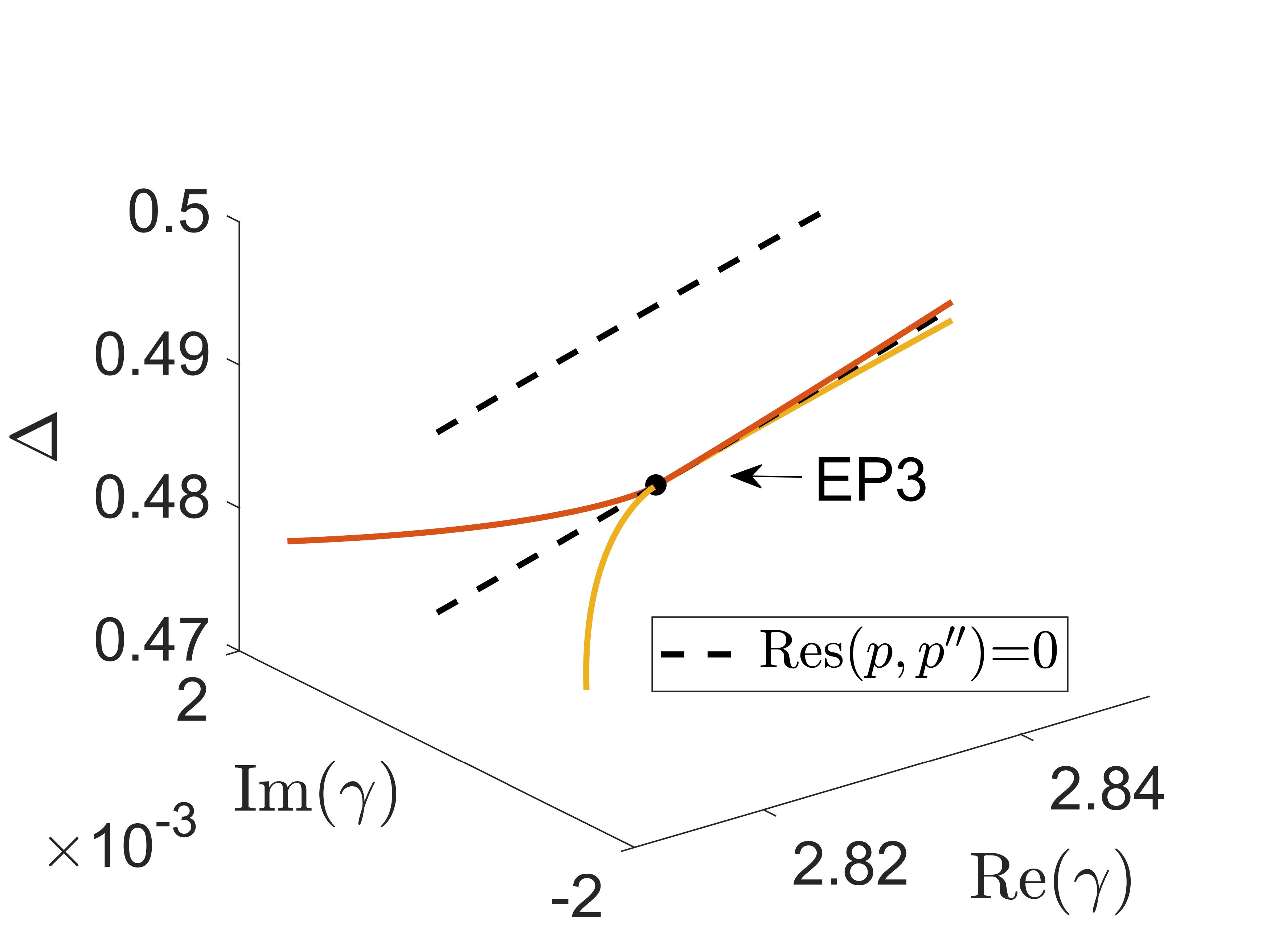
Figure S1: The intersection of ${\rm Res}(p,p^{\prime})=0$ and ${\rm Res}(p,p^{\prime\prime})=0$ at the EP3.

Appendix D IV. Stable paired exceptional points

In the main text, we mention that when the defect is placed at the midpoint of the chain, we can find a special EP, where all spectra coalesce in pairs, and that such a point is stable under perturbations. We refer to it a paired EP. Its location in parameter space can be calculated once we have the characteristic polynomial. Since the spectra coalesce in pairs, the characteristic polynomial can be simplified into the following form

$$p(\lambda)=q(\lambda)^{2}$$ (S32)

where every eigenvalue is doubly degenerate. This form can be achieved only at a special location of the defect. In terms of the sublattice index, we find that this happens when $s=\frac{N}{2}+1$ for $N$ even or at $s=\frac{N+1}{2}$ for $N$ odd.

We begin with the first case and set $N=2m$, and therefore $s=m+1$. Substituting into (S24),

$$p=U_{2m}+rU_{2m-1}+\frac{i\gamma\lambda}{1-\Delta^{2}}\left(U_{m}+rU_{m-1}\right)U_{m-1}.$$ (S33)

Using the properties of Chebyshev polynomials (S17), one can show that

$$U_{2m} =U_{m}^{2}-U_{m-1}^{2},$$ (S34)

$$U_{2m-1} =2U_{m}U_{m-1}-2QU_{m-1}^{2},$$

from which it follows that

$$p=U_{m}^{2}+\left(r^{2}-\frac{\lambda^{2}}{(1-\Delta)^{2}}+\frac{i\gamma\lambda r}{1-\Delta^{2}}\right)U_{m-1}^{2}+\left(2r+\frac{i\gamma\lambda}{1-\Delta^{2}}\right)U_{m}U_{m-1}.$$ (S35)

When $\gamma=2(1+\Delta)$, this polynomial is indeed a square

$$p=\left(U_{m}+\frac{i\lambda+1+\Delta}{1-\Delta}U_{m-1}\right)^{2}.$$ (S36)

This shows that the whole spectrum coalesces in pairs at the PEP2s $\gamma=2(1+\Delta)$. Also, the EP extends into an EL in 3D, which indicates its stability.

For the other case, we set $N=2m-1$, and therefore $s=m$, so that

$$p=U_{2m-1}+rU_{2m-2}+\frac{i\gamma\lambda}{1-\Delta^{2}}\left(U_{m-1}+rU_{m-2}\right)U_{m-1}.$$ (S37)

Similarly, expanding the Chebyshev polynomials,

$$p=\left(2Q+\frac{i\gamma\lambda}{1-\Delta^{2}}+r\right)U_{m-1}^{2}+\left(\frac{i\gamma\lambda r}{1-\Delta^{2}}-2\right)U_{m-1}U_{m-2}-rU_{m-2}^{2}.$$ (S38)

When $\gamma=2(1-\Delta)$, the polynomial is again a square

$$p=r\left(\frac{\lambda+i(1-\Delta)}{1+\Delta}U_{m-1}+iU_{m-2}\right)^{2},$$ (S39)

and a stable PEP2 appears at $\gamma=2(1-\Delta)$. However, as noted in the main text, in this case there is no EP4. Namely, the smaller value of $\gamma=2(1-\Delta)<2(1+\Delta)$ for positive $\Delta$ prevents the PEP2s from intersecting another EL in this case.

Appendix E V. Exceptional points of edge states

The Hermitian SSH chain in thermodynamic limits possesses two degenerate edge states, namely the left edge states and the right edge statesAsbóth et al. (2016)

$$|L\rangle=\sum_{l=1}^{N}a_{l}|2l-1\rangle,\quad|R\rangle=\sum_{l=1}^{N}b_{l}|2l\rangle$$ (S40)

where $a_{l}=(-1)^{l-1}a_{1}r^{-(l-1)},\quad b_{l}=(-1)^{N-l}b_{N}r^{-(N-l)}$, with normalized amplitudes given by

$$|a_{1}|^{2}=|b_{N}|^{2}=\frac{1-r^{-2}}{1-r^{-2N}}.$$ (S41)

The leading effects of defect on the edge states are captured by the effective two-level Hamiltonian

$$H_{\rm eff}=\left(\begin{array}[]{cc}\langle L|H|L\rangle&\langle L|H|R\rangle\\ \langle R|H|L\rangle&\langle R|H|R\rangle\end{array}\right)\equiv\left(\begin{array}[]{cc}\mathcal{E}_{L}&J\\ J^{*}&\mathcal{E}_{R}\end{array}\right),$$ (S42)

where

$$\mathcal{E}_{L}=-i\gamma|a_{s}|^{2},\mathcal{E}_{R}=0,J=(-1)^{N}(1-\Delta)a_{1}^{*}b_{N}r^{-(N-1)},$$ (S43)

Therefore, the eigenvalues of the effective Hamiltonian are

$$\lambda_{\rm edge,\pm}=\frac{1}{2}(\mathcal{E}_{L}\pm\sqrt{4|J|^{2}+\mathcal{E}_{L}^{2}})$$ (S44)

and the corresponding eigenstates are

$$\psi_{\pm}=\frac{1}{A}\left(J,\frac{1}{2}(\mathcal{E}_{L}\pm\sqrt{4|J|^{2}+\mathcal{E}_{L}^{2}})\right)^{T},$$ (S45)

where $A$ is a normalization factor,

$$A=\left\{\begin{aligned} &\sqrt{2}|J|&\gamma\leq\gamma_{\rm edge}\\ &\frac{1}{2}\sqrt{2i\mathcal{E}_{L}(i\mathcal{E}_{L}\pm\sqrt{-4|J|^{2}-\mathcal{E}_{L}^{2}}})&\gamma>\gamma_{\rm edge}\end{aligned}\right..$$ (S46)

The EPs lie at the coalescence of the eigenenergies, $4|J|^{2}+\mathcal{E}_{L}^{2}=0$, which correspond to

$$\gamma_{\rm edge}(\Delta)=\pm 2(1+\Delta)r^{2s-2-N}.$$ (S47)

Since we restrict the defect to be dissipative, only the positive solution is kept.

At finite length, the edge states overlap and give rise to the symmetric/anti-symmetric states $\frac{1}{\sqrt{2}}(|L\rangle\pm|R\rangle)$. When $\gamma\leq\gamma_{\rm edge}$, two eigenstates are

$$\psi_{\pm}=\frac{1}{\sqrt{2}}\left(1,e^{-i\varphi_{\pm}(\gamma)}\right)^{T},$$ (S48)

where $\varphi_{\pm}(\gamma)=\arctan\frac{\gamma}{\gamma_{\rm edge}^{2}-\gamma^{2}},\pi-\arctan\frac{\gamma}{\gamma_{\rm edge}^{2}-\gamma^{2}}$. At the EP the Hamiltonian is defective with only one eigenstate $\frac{1}{\sqrt{2}}(|L\rangle+e^{-i\frac{\pi}{2}}|R\rangle)$.

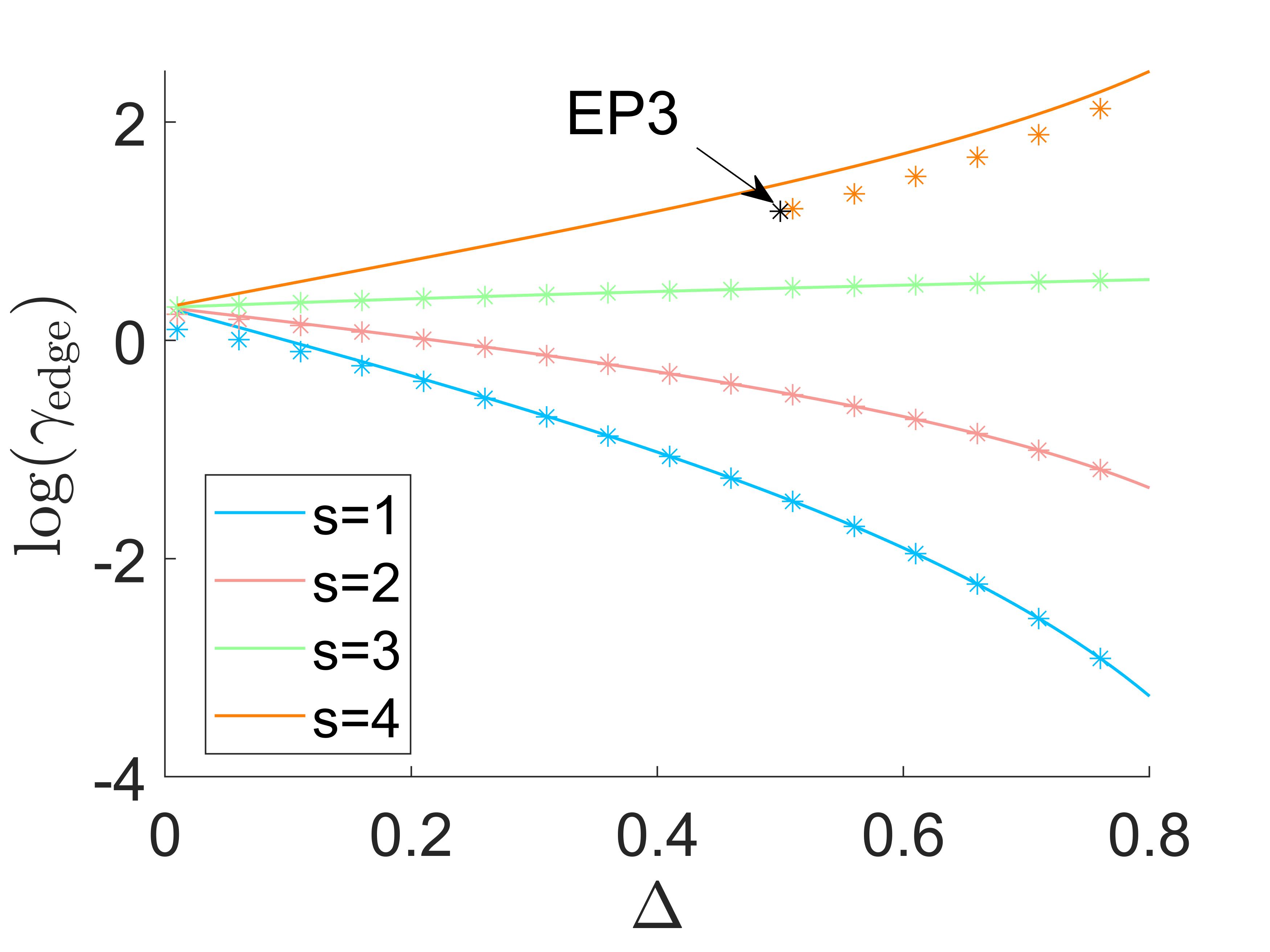
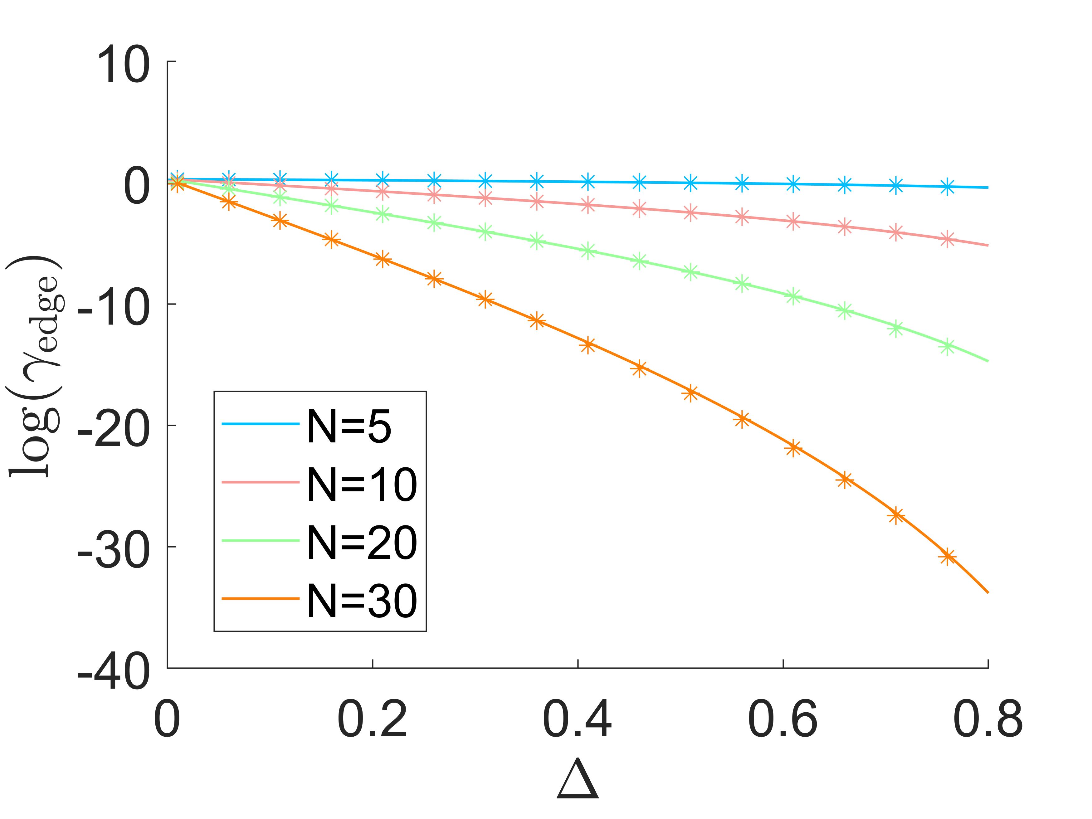
Figure S2: Comparison between analytical formulas (lines) and numerical results (points) for the location of edge EPs. (a) Colors: Different defect locations $2s-1$ at fixed chain length $2N=8$. (b) Colors: different chain lengths at fixed defect location $2s-1=5$.

For completeness, we estimate the mixing of edge states with scattering states, which was neglected above. Since the defect is located on the odd lattice sites, then to first order only the left edge state is modified,

$$|L^{\prime}\rangle=|L\rangle+\frac{i\gamma a_{s}}{N}\sum_{l=1}^{N}\sum_{k}e^{ik(s-l)-i\phi(k)}|2l\rangle+O(\gamma^{2}),$$ (S49)

$$\phi(k)=\tan^{-1}\frac{(1-\Delta)\sin k}{1+\Delta+(1-\Delta)\cos k},\quad\{k=\frac{2\pi n}{N-2}|n=0,1,\cdots,N-3\},$$ (S50)

where $k$ is the lattice momentum with discretized values at finite length. Thus, the two-level approximation is valid for $\gamma|a_{s}|\ll 1$. As a lower bound, the emergence of the edge EPs requires $\gamma_{edge}|a_{s}|\propto r^{s-N}\ll 1$. This is reflected in figures S2 & S2. Interestingly, when the defect is located at the right side of the midpoint, namely $s>N/2+1$, the numerical results are cut off at a range. This is because of the extension of the EP values out of the plane into complex region, after two EPs coalesce at a HOEP, in this case, an EP3.

Appendix F VI. Exceptional points of defect states

The defect states have the form

$$\psi_{l}=\left\{\begin{aligned} &A\exp(-\kappa|l-s|)\\ &B\exp(-\kappa|l-s+1|)\end{aligned}\right.\quad l=1,\cdots,N,$$ (S51)

where $\kappa$ is the localization rate with $\real(\kappa)>0$. Assuming an infinite chain, such an ansatz gives an eigenstate,

$$\sum_{j}H_{ij}\psi_{j}=\lambda\psi_{j}$$ (S52)

where

$$H_{ij}\equiv\langle i|H|j\rangle=-(1+(-1)^{i})\Delta)\delta_{i,j+1}-(1+(-1)^{j})\Delta)\delta_{i+1,j}-i\gamma\delta_{i,m}\delta_{j,m}$$ (S53)

is the Hamiltonian matrix. Since the chain is assumed infinite, different choices of the sublattice sites are equivalent, by translating the defect along the chain. For simplicity, we set $2s-1=0$,

$$\left\{\begin{aligned} &\lambda\psi_{2l-1}=-(1-\Delta)\psi_{2l-2}-(1+\Delta)\psi_{2l}\quad(l\in\mathbb{Z}),\\ &\lambda\psi_{0}=-(1+\Delta)\psi_{-1}-(1-\Delta)\psi_{1}-i\gamma\psi_{0},\\ &\lambda\psi_{2l}=-(1+\Delta)\psi_{2l-1}-(1-\Delta)\psi_{2l+1}\quad(l\in\mathbb{Z},l\neq 0).\end{aligned}\right.$$ (S54)

Only three independent equations in (S54) are left after substituting (S51), which give

$$\lambda^{2}=2(1-\Delta^{2})e^{-2\kappa}+2(1+\Delta^{2})-i\gamma\lambda,$$ (S55)

$$\lambda^{2}=(1-\Delta^{2})(e^{2\kappa}+e^{-2\kappa})+2(1+\Delta^{2}),$$

and the relation for the coefficients $A$ and $B$ is

$$Be^{-\kappa}=-(1-\Delta)e^{-2\kappa}-(1+\Delta)A.$$ (S56)

Let $x=e^{2\kappa},y=x+1/x$. We can determine $y$ from (S55),

$$y^{2}+\frac{\gamma^{2}}{(1-\Delta^{2})}y+\frac{2\gamma^{2}(1+\Delta^{2})}{(1-\Delta^{2})^{2}}-4=0,$$ (S57)

with the solutions

$$y_{\pm}=\frac{-\gamma^{2}\pm\sqrt{(\gamma^{2}-4(1-\Delta)^{2})(\gamma^{2}-4(1+\Delta)^{2})}}{2(1-\Delta^{2})}.$$ (S58)

Substituting (S58) into (S55), we obtain the exact form of eigenvalues $\lambda$ shown in the main text. These predict EPs at $\gamma_{\rm defect}=2(1\pm\Delta)$ and $\gamma_{\rm defect}=-2(1\pm\Delta)$. Similarly, only the EPs with $\real(\gamma)>0$ correspond to disspative defect.

However, not all solutions satisfy our localized ansatz $\real(\kappa)>0$. To be more specific, we separate the real and imaginary parts of $\kappa$ as $\kappa=\kappa_{R}+i\kappa_{I}$. For localized states, we require $\kappa_{R}>0$. $y=e^{2\kappa}+e^{-2\kappa}$ can be simplified as

$${\rm Re}(y)=2\cosh(2\kappa_{R})\cos(2\kappa_{I}),$$ (S59)

$${\rm Im}(y)=2\sinh(2\kappa_{R})\sin(2\kappa_{I}).$$

When $\gamma\leq 2(1-\Delta)$, $\imaginary(y)$ is always $0$, corresponding to two solutions $\kappa_{R}=0$ or $\kappa_{I}=n\pi/2$. Since $|\real(y_{\pm})|\leq 2$, the solutions are $\kappa_{R}=0$ and $\kappa_{I}=\frac{1}{2}\arccos(\frac{1}{2}\real(y_{\pm}))$. Here, $\kappa$ is purely imaginary. Therefore, the EP located at $\gamma=2(1-\Delta)$ corresponds to the coalescence of the scattering states within one band.

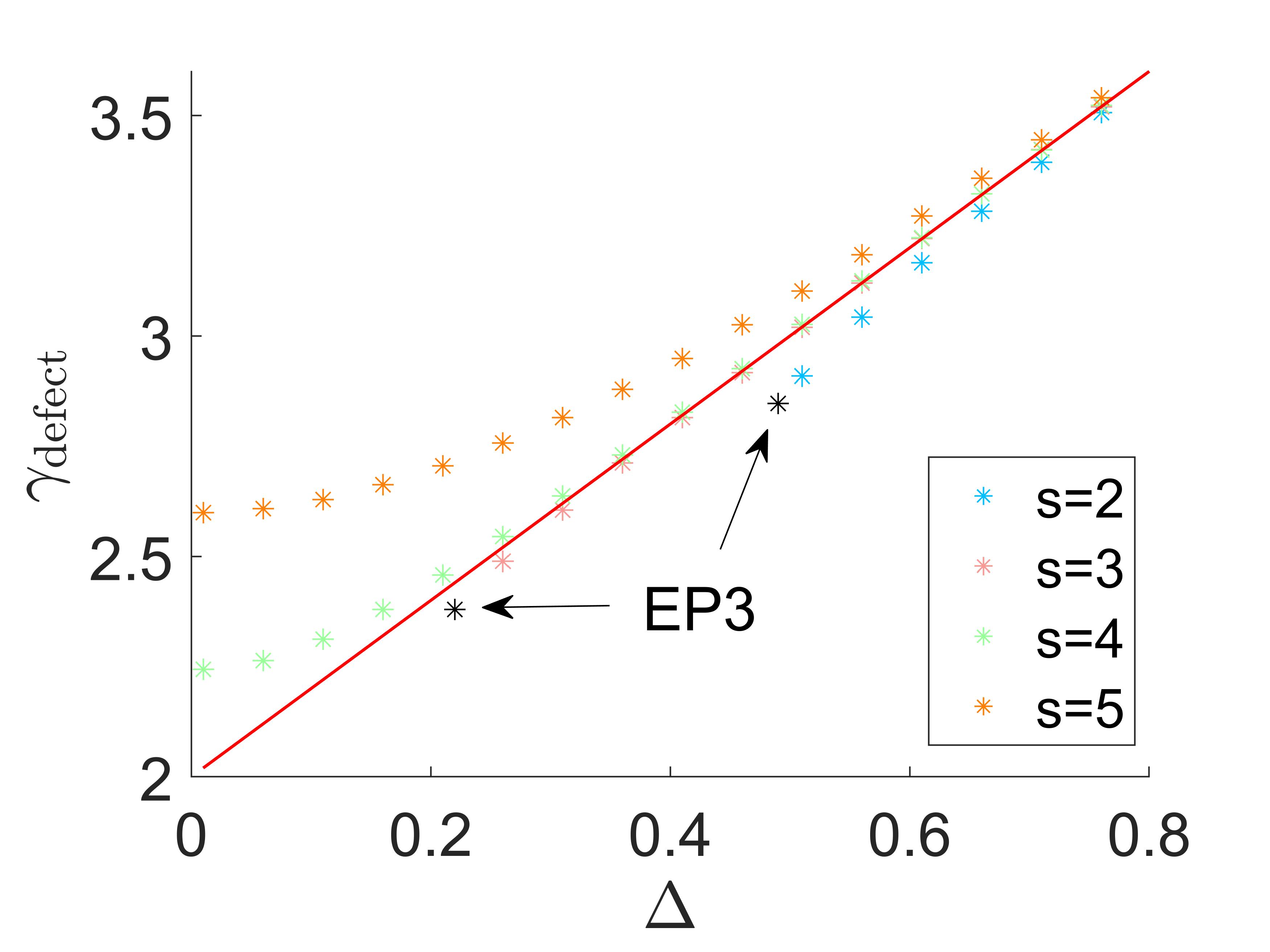
Figure S3: Comparison between analytical formula (line) and numerical results (points) for the location of defect EPs. Colors correspond to different defect locations $2s-1$ at fixed chain length $2N=10$.

When $2(1-\Delta)<\gamma<2(1+\Delta)$,

$$\cosh(2\kappa_{R})\cos(2\kappa_{I})=-\frac{\gamma^{2}}{4(1-\Delta^{2})}<-1,$$ (S60)

$$\sinh(2\kappa_{R})\sin(2\kappa_{I})=\pm\frac{\sqrt{(\gamma^{2}-4(1-\Delta)^{2})(4(1+\Delta)^{2}-\gamma^{2})}}{4(1-\Delta^{2})},$$

so that $\kappa_{R}>0$. At the EP $\gamma=2(1+\Delta)$, the solutions are $\cosh(2\kappa_{R})=r,\kappa_{I}=\pm\pi/2$. Two mid-gap defect states coalesce.

Finally, when $\gamma>2(1+\Delta)$, $\imaginary(y)$ is always $0$, and $\real(|y_{\pm}|)>2$. We find the solutions are $\kappa_{I}=n\pi/2$ and $\kappa_{R}=\frac{1}{2}\cosh^{-1}(\frac{1}{2}\real(|y_{\pm}|))$. Here, two defect states with different localization rates appear, and the energy gap between the them becomes fully imaginary.

Note that, in solving for the defect states, we for simplicity assumed an infinite chain. In a finite chain, the wave functions are truncated near the edge, with approximate form

$$\psi_{i}^{\rm cut}\sim\left\{\begin{aligned} &\psi_{i}\quad i\in\{1,\cdots,2N\}\\ &0\quad\ \rm else\end{aligned}\right.,$$ (S61)

where in the first line $\psi_{i}$ are the eigenstates we solved for above. The truncation leads to an energy difference

$$\Delta\lambda\sim\max\{|\psi_{0}|^{2},|\psi_{2N+1}|^{2}\},$$ (S62)

where

$$|\psi_{0}|^{2}=|B|^{2}\exp(-2\kappa_{R}(s-1)),|\psi_{2N+1}|^{2}=|A|^{2}\exp(-2\kappa_{R}(N+1-s)).$$ (S63)

The energy difference indicates that the results are more accurate when the defect is far from the boundary, or when the wave functions are more strongly localized. If the defect is closer to the left boundary, the approximation is valid for large $\gamma|a_{s}|^{-1}\gg 1$, as shown in figure S3.

Appendix G VII. Exceptional points of hybridization of edge states and defect states

There is another possibility when a defect state coalesces with an edge state. The existence of such an EP becomes clear by examining the eigenvalues of the four localized states we obtained above. When $\gamma>\max\{\gamma_{\rm edge},\gamma_{\rm defect}\}$, the four eigenvalues are purely imaginary. When $\gamma\gg\max\{\gamma_{\rm edge},\gamma_{\rm defect}\}$, these have the approximate form

$$\lambda_{\rm edge}\approx-i\gamma|a_{s}|^{2},-i|J|\frac{\gamma_{\rm edge}}{2\gamma},\quad\lambda_{\rm impu}\approx-i\gamma,-i\frac{4\Delta}{\gamma}.$$ (S64)

The gap between one of the edge states and one of the localized states closes at $\gamma_{\rm mixed}=\sqrt{4\Delta}|a_{s}|^{-1}$. After substituting the exact form of $|a_{s}|$, we arrive at the $\gamma_{\rm mixed}$ in the main text. However, since the eigenenergies of the localized states are largely shifted beyond the approximation region $\gamma|a_{s}|\ll 1$, the prediction only agrees with the exact results by order of $r^{s-1}$ [see figure S4].

At the points where $\gamma_{\rm mixed}$ meets with $\gamma_{\rm edge}$ or $\gamma_{\rm defect}$, HOEPs emerge. This also explains the cut off in the plots of the numerically obtained EP values in figures. S2-S4, where after coalescing at a HOEP the EP2s extend into complex region, out of the plane in these pictures. Since $\gamma_{\rm mixed}$ may coalesce with different EPs when varying the defect location, the values of the HOEP can be solved by two different equations. Specifically, we solve

$$\left\{\begin{aligned} &\gamma_{\rm mixed}=\gamma_{\rm defect},&\gamma_{\rm edge}<\gamma_{\rm defect}\\ &\gamma_{\rm mixed}=\gamma_{\rm edge},&\gamma_{\rm edge}>\gamma_{\rm defect}\end{aligned}\right.\Rightarrow\left\{\begin{aligned} &r^{s-1}\sqrt{\frac{1-r^{-2N}}{1-r^{-2}}\cdot 4\Delta}=2(1+\Delta),&s<\frac{N}{2}+1\\ &r^{s-1}\sqrt{\frac{1-r^{-2N}}{1-r^{-2}}\cdot 4\Delta}=2(1-\Delta)r^{2s-1-N},&s>\frac{N}{2}+1\end{aligned}\right.$$ (S65)

where the choice of different equation is only determined by the relation between defect location $s$ and the sublattice sites $N$. A different case appears at $s=\frac{N}{2}+1$, where $N$ is even. At this point, we have $\gamma_{\rm edge}=\gamma_{\rm defect}$, which means they have exactly the same value and becomes degenerate. Therefore, the corresponding HOEP is actually an EP4, where all the localized states coalesce.

Figure S4: Comparison between analytical formulas (lines) and numerical results (points) for the location of mixed EPs. Colors correspond to different defect locations $2s-1$ at fixed chain length $2N=10$.

References

- Heiss (2012) W. Heiss, “The physics of exceptional points,” Journal of Physics A: Mathematical and Theoretical 45, 444016 (2012).
- Heiss (2004) W. Heiss, “Exceptional points of non-hermitian operators,” Journal of Physics A: Mathematical and General 37, 2455 (2004).
- Berry (2004) M. Berry, “Physics of Nonhermitian Degeneracies,” Czechoslovak Journal of Physics 54, 1039–1047 (2004).
- Yuto Ashida and Ueda (2020) Z. G. Yuto Ashida and M. Ueda, “Non-hermitian physics,” Advances in Physics 69, 249–435 (2020).
- Bergholtz et al. (2021) E. J. Bergholtz, J. C. Budich, and F. K. Kunst, “Exceptional topology of non-hermitian systems,” Rev. Mod. Phys. 93, 015005 (2021).
- Stehmann et al. (2004) T. Stehmann, W. Heiss, and F. Scholtz, “Observation of exceptional points in electronic circuits,” Journal of Physics A: Mathematical and General 37, 7813 (2004).
- Dembowski et al. (2001) C. Dembowski, H.-D. Gräf, H. L. Harney, A. Heine, W. D. Heiss, H. Rehfeld, and A. Richter, “Experimental observation of the topological structure of exceptional points,” Phys. Rev. Lett. 86, 787–790 (2001).
- Shi et al. (2016) C. Shi, M. Dubois, Y. Chen, L. Cheng, H. Ramezani, Y. Wang, and X. Zhang, “Accessing the exceptional points of parity-time symmetric acoustics,” Nature communications 7, 11110 (2016).
- Özdemir et al. (2019) Ş. K. Özdemir, S. Rotter, F. Nori, and L. Yang, “Parity–time symmetry and exceptional points in photonics,” Nature materials 18, 783–798 (2019).
- Miri and Alu (2019) M.-A. Miri and A. Alu, “Exceptional points in optics and photonics,” Science 363, eaar7709 (2019).
- Arouca et al. (2023) R. Arouca, J. Cayao, and A. M. Black-Schaffer, “Topological superconductivity enhanced by exceptional points,” Phys. Rev. B 108, L060506 (2023).
- Li et al. (2023a) Z.-Z. Li, W. Chen, M. Abbasi, K. W. Murch, and K. B. Whaley, “Speeding up entanglement generation by proximity to higher-order exceptional points,” Phys. Rev. Lett. 131, 100202 (2023a).
- Bu et al. (2023) J.-T. Bu, J.-Q. Zhang, G.-Y. Ding, J.-C. Li, J.-W. Zhang, B. Wang, W.-Q. Ding, W.-F. Yuan, L. Chen, i. m. c. K. Özdemir, F. Zhou, H. Jing, and M. Feng, “Enhancement of quantum heat engine by encircling a liouvillian exceptional point,” Phys. Rev. Lett. 130, 110402 (2023).
- Yao and Wang (2018) S. Yao and Z. Wang, “Edge states and topological invariants of non-hermitian systems,” Phys. Rev. Lett. 121, 086803 (2018).
- Lee (2016) T. E. Lee, “Anomalous edge state in a non-hermitian lattice,” Phys. Rev. Lett. 116, 133903 (2016).
- Xiong (2018) Y. Xiong, “Why does bulk boundary correspondence fail in some non-hermitian topological models,” Journal of Physics Communications 2, 035043 (2018).
- Kunst et al. (2018) F. K. Kunst, E. Edvardsson, J. C. Budich, and E. J. Bergholtz, “Biorthogonal bulk-boundary correspondence in non-hermitian systems,” Phys. Rev. Lett. 121, 026808 (2018).
- Xiao et al. (2020) L. Xiao, T. Deng, K. Wang, G. Zhu, Z. Wang, W. Yi, and P. Xue, “Non-hermitian bulk–boundary correspondence in quantum dynamics,” Nature Physics 16, 761–766 (2020).
- Helbig et al. (2020) T. Helbig, T. Hofmann, S. Imhof, M. Abdelghany, T. Kiessling, L. Molenkamp, C. Lee, A. Szameit, M. Greiter, and R. Thomale, “Generalized bulk–boundary correspondence in non-hermitian topolectrical circuits,” Nature Physics , 1–4 (2020).
- Ghatak et al. (2020) A. Ghatak, M. Brandenbourger, J. Van Wezel, and C. Coulais, “Observation of non-hermitian topology and its bulk–edge correspondence in an active mechanical metamaterial,” Proceedings of the National Academy of Sciences 117, 29561–29568 (2020).
- Borgnia et al. (2020) D. S. Borgnia, A. J. Kruchkov, and R.-J. Slager, “Non-hermitian boundary modes and topology,” Phys. Rev. Lett. 124, 056802 (2020).
- Li et al. (2021) L. Li, C. H. Lee, and J. Gong, “Impurity induced scale-free localization,” Communications Physics 4, 42 (2021).
- Okuma and Sato (2023) N. Okuma and M. Sato, “Non-Hermitian topological phenomena: A review,” Annu. Rev. Condens. Matter Phys. 14, 83–107 (2023).
- Jana and Sirota (2023) S. Jana and L. Sirota, “Emerging exceptional point with breakdown of the skin effect in non-hermitian systems,” Phys. Rev. B 108, 085104 (2023).
- Tzortzakakis et al. (2022) A. F. Tzortzakakis, A. Katsaris, N. E. Palaiodimopoulos, P. A. Kalozoumis, G. Theocharis, F. K. Diakonos, and D. Petrosyan, “Topological edge states of the -symmetric su-schrieffer-heeger model: An effective two-state description,” Phys. Rev. A 106, 023513 (2022).
- Schomerus (2013) H. Schomerus, “Topologically protected midgap states in complex photonic lattices,” Opt. Lett. 38, 1912–1914 (2013).
- Poli et al. (2015) C. Poli, M. Bellec, U. Kuhl, F. Mortessagne, and H. Schomerus, “Selective enhancement of topologically induced interface states in a dielectric resonator chain,” Nature communications 6, 6710 (2015).
- Guo et al. (2023a) C.-X. Guo, X. Wang, H. Hu, and S. Chen, “Accumulation of scale-free localized states induced by local non-hermiticity,” Phys. Rev. B 107, 134121 (2023a).
- Li et al. (2023b) B. Li, H.-R. Wang, F. Song, and Z. Wang, “Scale-free localization and symmetry breaking from local non-hermiticity,” Phys. Rev. B 108, L161409 (2023b).
- Molignini et al. (2023) P. Molignini, O. Arandes, and E. J. Bergholtz, “Anomalous skin effects in disordered systems with a single non-hermitian impurity,” Phys. Rev. Res. 5, 033058 (2023).
- Ding et al. (2022) K. Ding, C. Fang, and G. Ma, “Non-hermitian topology and exceptional-point geometries,” Nature Reviews Physics 4, 745–760 (2022).
- Patil et al. (2022) Y. S. Patil, J. Höller, P. A. Henry, C. Guria, Y. Zhang, L. Jiang, N. Kralj, N. Read, and J. G. Harris, “Measuring the knot of non-hermitian degeneracies and non-commuting braids,” Nature 607, 271–275 (2022).
- Delplace et al. (2021) P. Delplace, T. Yoshida, and Y. Hatsugai, “Symmetry-protected multifold exceptional points and their topological characterization,” Phys. Rev. Lett. 127, 186602 (2021).
- Mandal and Bergholtz (2021) I. Mandal and E. J. Bergholtz, “Symmetry and higher-order exceptional points,” Phys. Rev. Lett. 127, 186601 (2021).
- Carlström et al. (2019) J. Carlström, M. Stålhammar, J. C. Budich, and E. J. Bergholtz, “Knotted non-Hermitian metals,” Physical Review B 99, 161115 (2019).
- Zhang et al. (2021) X. Zhang, G. Li, Y. Liu, T. Tai, R. Thomale, and C. H. Lee, “Tidal surface states as fingerprints of non-Hermitian nodal knot metals,” Communications Physics 4, 1–10 (2021).
- Hu and Zhao (2021) H. Hu and E. Zhao, “Knots and non-hermitian bloch bands,” Phys. Rev. Lett. 126, 010401 (2021).
- Zhong et al. (2018) Q. Zhong, M. Khajavikhan, D. N. Christodoulides, and R. El-Ganainy, “Winding around non-hermitian singularities,” Nature communications 9, 4808 (2018).
- Hu et al. (2022) H. Hu, S. Sun, and S. Chen, “Knot topology of exceptional point and non-hermitian no-go theorem,” Phys. Rev. Res. 4, L022064 (2022).
- Rui et al. (2019) W. B. Rui, Y. X. Zhao, and A. P. Schnyder, “Topology and exceptional points of massive dirac models with generic non-hermitian perturbations,” Phys. Rev. B 99, 241110 (2019).
- Luitz and Piazza (2019) D. J. Luitz and F. Piazza, “Exceptional points and the topology of quantum many-body spectra,” Phys. Rev. Res. 1, 033051 (2019).
- Zhou et al. (2018) H. Zhou, C. Peng, Y. Yoon, C. W. Hsu, K. A. Nelson, L. Fu, J. D. Joannopoulos, M. Soljačić, and B. Zhen, “Observation of bulk fermi arc and polarization half charge from paired exceptional points,” Science 359, 1009–1012 (2018).
- Guo et al. (2023b) C.-X. Guo, S. Chen, K. Ding, and H. Hu, “Exceptional non-abelian topology in multiband non-hermitian systems,” Phys. Rev. Lett. 130, 157201 (2023b).
- König et al. (2023) J. L. K. König, K. Yang, J. C. Budich, and E. J. Bergholtz, “Braid-protected topological band structures with unpaired exceptional points,” Phys. Rev. Res. 5, L042010 (2023).
- Wojcik et al. (2022) C. C. Wojcik, K. Wang, A. Dutt, J. Zhong, and S. Fan, “Eigenvalue topology of non-hermitian band structures in two and three dimensions,” Phys. Rev. B 106, L161401 (2022).
- Lin et al. (2019) S. Lin, L. Jin, and Z. Song, “Symmetry protected topological phases characterized by isolated exceptional points,” Phys. Rev. B 99, 165148 (2019).
- González and Molina (2017) J. González and R. A. Molina, “Topological protection from exceptional points in weyl and nodal-line semimetals,” Phys. Rev. B 96, 045437 (2017).
- Ryu et al. (2012) J.-W. Ryu, S.-Y. Lee, and S. W. Kim, “Analysis of multiple exceptional points related to three interacting eigenmodes in a non-hermitian hamiltonian,” Phys. Rev. A 85, 042101 (2012).
- Kozii and Fu (2017) V. Kozii and L. Fu, “Non-hermitian topological theory of finite-lifetime quasiparticles: prediction of bulk fermi arc due to exceptional point,” arXiv preprint arXiv:1708.05841 (2017), https://doi.org/10.48550/arXiv.1708.05841.
- Hu et al. (2023) J. Hu, R.-Y. Zhang, Y. Wang, X. Ouyang, Y. Zhu, H. Jia, and C. T. Chan, “Non-Hermitian swallowtail catastrophe revealing transitions among diverse topological singularities,” Nature Physics 19, 1098–1103 (2023).
- Yang et al. (2023) K. Yang, Z. Li, J. L. K. König, L. Rødland, M. Stålhammar, and E. J. Bergholtz, “Homotopy, Symmetry, and Non-Hermitian Band Topology,” (2023), 10.48550/arXiv.2309.14416.
- Budich et al. (2019) J. C. Budich, J. Carlström, F. K. Kunst, and E. J. Bergholtz, “Symmetry-protected nodal phases in non-Hermitian systems,” Physical Review B 99, 041406 (2019).
- Kawabata et al. (2019) K. Kawabata, T. Bessho, and M. Sato, “Classification of exceptional points and non-hermitian topological semimetals,” Phys. Rev. Lett. 123, 066405 (2019).
- Kimura et al. (2019) K. Kimura, T. Yoshida, and N. Kawakami, “Chiral-symmetry protected exceptional torus in correlated nodal-line semimetals,” Physical Review B 100, 115124 (2019).
- Okugawa and Yokoyama (2019) R. Okugawa and T. Yokoyama, “Topological exceptional surfaces in non-Hermitian systems with parity-time and parity-particle-hole symmetries,” Physical Review B 99, 041202 (2019).
- Szameit et al. (2011) A. Szameit, M. C. Rechtsman, O. Bahat-Treidel, and M. Segev, “-symmetry in honeycomb photonic lattices,” Physical Review A 84, 021806 (2011).
- Yoshida et al. (2019) T. Yoshida, R. Peters, N. Kawakami, and Y. Hatsugai, “Symmetry-protected exceptional rings in two-dimensional correlated systems with chiral symmetry,” Physical Review B 99, 121101 (2019).
- Yang and Mandal (2023) K. Yang and I. Mandal, “Enhanced eigenvector sensitivity and algebraic classification of sublattice-symmetric exceptional points,” Phys. Rev. B 107, 144304 (2023).
- Zhou et al. (2019) H. Zhou, J. Y. Lee, S. Liu, and B. Zhen, “Exceptional surfaces in -symmetric non-Hermitian photonic systems,” Optica 6, 190–193 (2019).
- Stålhammar and Bergholtz (2021) M. Stålhammar and E. J. Bergholtz, “Classification of exceptional nodal topologies protected by symmetry,” Physical Review B 104, L201104 (2021).
- Crippa et al. (2021) L. Crippa, J. C. Budich, and G. Sangiovanni, “Fourth-order exceptional points in correlated quantum many-body systems,” Physical Review B 104, L121109 (2021).
- Wang et al. (2023) K. Wang, L. Xiao, H. Lin, W. Yi, E. J. Bergholtz, and P. Xue, “Experimental simulation of symmetry-protected higher-order exceptional points with single photons,” Science Advances 9, eadi0732 (2023).
- Wojcik et al. (2020) C. C. Wojcik, X.-Q. Sun, T. c. v. Bzdušek, and S. Fan, “Homotopy characterization of non-hermitian hamiltonians,” Phys. Rev. B 101, 205417 (2020).
- Li and Mong (2021) Z. Li and R. S. K. Mong, “Homotopical characterization of non-hermitian band structures,” Phys. Rev. B 103, 155129 (2021).
- Heeger et al. (1988) A. J. Heeger, S. Kivelson, J. R. Schrieffer, and W. P. Su, “Solitons in conducting polymers,” Rev. Mod. Phys. 60, 781–850 (1988).
- Janson (2007) S. Janson, “Resultant and discriminant of polynomials,” Notes, September 22 (2007).
- Woody (2016) H. Woody, “Polynomial resultants,” GNU operating system (2016).
- Sayyad and Kunst (2022) S. Sayyad and F. K. Kunst, “Realizing exceptional points of any order in the presence of symmetry,” Phys. Rev. Res. 4, 023130 (2022).
- (69) See Supplementary Material for details on (I) the introduction to the general method to obtain degenerate points, (II) the derivation of the characteristic polynomial of the Hamiltonian (1), (III) the derivation of exceptional lines in figure 2, (IV) the derivation of stable paired exceptional points, (V) the derivation of exceptional points of edge states (8), (VI) the derivation of exceptional points of defect states (11) and (VII) the derivation of exceptional points of hybridization of edge states and defect states (12).
- Mason and Handscomb (2002) J. C. Mason and D. C. Handscomb, Chebyshev polynomials (CRC press, 2002).
- Dykhne (1960) A. Dykhne, “Quantum transitions in the adiabatic approximation,” Sov. Phys. JETP 11, 411 (1960).
- Hwang and Pechukas (1977) J.-T. Hwang and P. Pechukas, “The adiabatic theorem in the complex plane and the semiclassical calculation of nonadiabatic transition amplitudes,” The Journal of Chemical Physics 67, 4640–4653 (1977).
- Wang et al. (2022) W.-Y. Wang, B. Sun, and J. Liu, “Adiabaticity in nonreciprocal landau-zener tunneling,” Physical Review A 106, 063708 (2022).
- Cardoso (2023) G. Cardoso, “A landau-zener formula for the adiabatic gauge potential,” (2023), 10.48550/arXiv.2303.12066.
- Fox and Neuwirth (1962) R. Fox and L. Neuwirth, “The braid groups,” Mathematica Scandinavica 10, 119–126 (1962).
- Birman (1974) J. S. Birman, Braids, links, and mapping class groups, 82 (Princeton University Press, 1974).
- Ding et al. (2016) K. Ding, G. Ma, M. Xiao, Z. Q. Zhang, and C. T. Chan, “Emergence, coalescence, and topological properties of multiple exceptional points and their experimental realization,” Phys. Rev. X 6, 021007 (2016).
- Doppler et al. (2016) J. Doppler, A. A. Mailybaev, J. Böhm, U. Kuhl, A. Girschik, F. Libisch, T. J. Milburn, P. Rabl, N. Moiseyev, and S. Rotter, “Dynamically encircling an exceptional point for asymmetric mode switching,” Nature 537, 76–79 (2016).
- Joglekar et al. (2010) Y. N. Joglekar, D. Scott, M. Babbey, and A. Saxena, “Robust and fragile -symmetric phases in a tight-binding chain,” Phys. Rev. A 82, 030103 (2010).
- Burke et al. (2020) P. C. Burke, J. Wiersig, and M. Haque, “Non-hermitian scattering on a tight-binding lattice,” Phys. Rev. A 102, 012212 (2020).
- Król et al. (2022) M. Król, I. Septembre, P. Oliwa, M. Kȩdziora, K. Łempicka-Mirek, M. Muszyński, R. Mazur, P. Morawiak, W. Piecek, P. Kula, et al., “Annihilation of exceptional points from different dirac valleys in a 2d photonic system,” Nature Communications 13, 5340 (2022).
- Lin et al. (2023) R. Lin, T. Tai, L. Li, and C. H. Lee, “Topological non-hermitian skin effect,” Frontiers of Physics 18, 53605 (2023).
- Cheng et al. (2022) J. Cheng, X. Zhang, M.-H. Lu, and Y.-F. Chen, “Competition between band topology and non-hermiticity,” Phys. Rev. B 105, 094103 (2022).
- Zhu et al. (2021) W. Zhu, W. X. Teo, L. Li, and J. Gong, “Delocalization of topological edge states,” Phys. Rev. B 103, 195414 (2021).
- Hasan and Kane (2010) M. Z. Hasan and C. L. Kane, “Colloquium: Topological insulators,” Rev. Mod. Phys. 82, 3045–3067 (2010).
- Qi and Zhang (2011) X.-L. Qi and S.-C. Zhang, “Topological insulators and superconductors,” Rev. Mod. Phys. 83, 1057–1110 (2011).
- Chiu et al. (2016) C.-K. Chiu, J. C. Y. Teo, A. P. Schnyder, and S. Ryu, “Classification of topological quantum matter with symmetries,” Rev. Mod. Phys. 88, 035005 (2016).
- Asbóth et al. (2016) J. K. Asbóth, L. Oroszlány, and A. Pályi, A Short Course on Topological Insulators (Springer International Publishing, 2016).