Device-Independent Quantum Secure Direct Communication Under Non-Markovian Quantum Channels

Abstract

Device-independent quantum secure direct communication (DI-QSDC) is a promising primitive in quantum cryptography aimed towards addressing the problems of device imperfections and key management. However, significant effort is required to tackle practical challenges such as the distance limitation due to decohering effects of quantum channels. Here, we explore the constructive effect of non-Markovian noise to improve the performance of DI-QSDC. Considering two different environmental dynamics modeled by the amplitude damping and the dephasing channels, we show that for both cases non-Markovianty leads to a considerable improvement over Markovian dynamics in terms of three benchmark performance criteria of the DI-QSDC task. Specifically, we find that non-Markovian noise (i) enhances the protocol security measured by Bell-violation, (ii) leads to a lower quantum bit error rate, and (iii) enables larger communication distances by increasing the capacity of secret communication.

I Introduction

In classical cryptography, secure communication is primarily based on the computational complexity of one-way mathematical functions Rivest78 . The computational complexity reduces using the quantum resources and the algorithms like Shor’s and Grover Shor94 ; Grover96 ; Long01 thus raising concern on the security of the traditional communication protocols in the post-quantum world. Quantum problems have quantum solutions giving emergence to quantum cryptography Gisin02 . Several quantum communication tasks have been proposed, including quantum teleportation bennet93 , quantum key distribution (QKD) Bennet92 ; BB84 ; ekert91 , quantum secure direct communication Long02 , and others Hillery . The unique feature to detect the presence of eavesdropper distinguishes quantum communication tasks from their classical counterparts.

Quantum cryptography and quantum sensing Dengen17 are among the most advanced sectors under quantum technologies. Non-classical resources like entanglement ent , steering steer and Bell-nonlocality bell are the primary driving forces for these technologies followed by advancements in the single photon sources and detectors Eisaman11 . Quantum key distribution is the most celebrated protocol under quantum cryptography with several successful trials and commercial products available currently Acin07 ; Pawlowski10 ; Pramanik ; vazirani ; Huang18 ; Tang19 ; Jan20 ; Farkas21 ; Jaskaran ; Nadlinger21 ; Yash21 ; Bera23 . However, loophole free self-testing, secure key management, migration and side channel attacks remain challenging hindrances Takahashi19 .

Quantum secure direct communication (QSDC) has been put forward to address some of these challenges Wootters92 ; Long02 . QSDC does not require key management, and hence, it is advantageous compared to quantum key distribution (QKD) and traditional classical communications Pan20 . However, component imperfections and implementation loopholes in realistic setups can compromise the security of QSDC protocol, as well. In this context, device-independent QSDC has been recently proposed LanZhou ; LanZhou1 ; LanZhou23 ; WeiZhang just like DI-QKD Metger21 ; Xu21 . QSDC is regarded to have a huge potential for future communication networks and in developing a quantum internet Singh21 .

One cannot escape the interaction with the ubiquitous environment during experimental or commercial realizations of such communication tasks. During this interaction, quantum correlations, in general, get destroyed, thereby creating obstacles in the successful implementation or long term execution of such tasks. Impact of the noise on quantum correlations has been studied extensively suddendeathent . Entanglement sudden death (ESD) may occur under interaction with dephasing channel noise suddendeathent . On the other hand, under certain circumstances, a controlled environment may also aid in preservation of quantum correlations Badziag2000 ; Bandyopadhyay02 ; GMN2006 ; Rivu21 . In particular, revival of entanglement has been reported under non-Markovian channel interaction RLF17 ; nonMarkoent ; Rivu22 .

Techniques to mitigate the effect of noise on quantum correlations have been explored in the literature. For example, employing a scheme of weak measurements enables preservation of various kinds of quantum correlations such as teleportation fidelity PM13 , quantum secret key rate DGPM2017 , and quantum non-bilocal correlations Gupta18 under the effect of the amplitude damping channel GGM21 . Several instances have been found where the noise has constructive effect on the teleportation fidelity and the coding capacity Rivu21 . Most significantly, non-Markovian noise has been indicated to play a key role in the enhancement of quantum correlations in wide arenas such as quantum information nminfo ; Rivu22 and metrology nmmetro , prompting development of resource theoretic frameworks for non-Markovianity Samya1 . Furthermore, the development of advanced experimental technology may enable an open system to be driven from a Markovian to a non-Markovian regime nphys2011 .

The above examples of constructive behaviour of the noise raises the question as to whether non-Markovian noise can improve the figure of merit for a general quantum communication task such as quantum secure direct communication ? We answer this question affirmatively in this work. In the present paper, we analyse the effect of the non-Markovian noise modelled by both the amplitude damping channel and the phase damping channel on the performance of a device-independent quantum secure direct communication task (DI-QKD). In our protocol, the entangled pair of quantum particles interact with the channel noise. Through our analysis we obtain a range of model parameters for which the non-Markovian noise enables better preservation of the nonclassical behaviour compared to the Markovian counterpart for the amplitude damping as well as dephasing channel noise.

The paper is organized as follows. In Sec. II, we present a brief overview of the general Device-Independent Quantum secure direct communication (DI-QSDC) task along with the description of the open quantum systems and non-Markovian amplitude damping and dephasing quantum channels. In Sec. III, we consider a specific QSDC task where both the entangled quantum particles interact with the damping channel. In Sec. IV, we analyse the effect of the non-Markovian channels on the performance of the QSDC. Lastly, in Sec. V, we present a summary of our results and concluding remarks.

II Preliminaries

In this Section, we will first recapitulate the notion of the quantum secure direct communication (QSDC). Then, we will consider the dynamics of open quantum system and non-Markovian quantum channels under consideration for the present work.

II.1 General QSDC protocol

Quantum Secure Direct Communication (QSDC) facilitates the transmission of confidential messages through a quantum channel without the need for a pre-shared key. As shown in fig-(1), authorized parties like Alice, the sender, encode messages using quantum states, and Bob, the receiver, decodes them through specific measurements and security checks. The security of this method relies heavily on the no-cloning theorem and the utilization of entanglement. Depending on the chosen non-classical resource, encoding and decoding scheme, QSDC can be either of the prepare-measure type Deng04 or the entanglement-based type Deng03 . This approach offers a robust guarantee of message confidentiality, even when potential eavesdroppers like Eve are present, without the requirement of establishing a shared key in advance. QSDC harnesses the principles of quantum mechanics to ensure inherently secure communication, making it a highly promising technology for the future of secure data exchange.

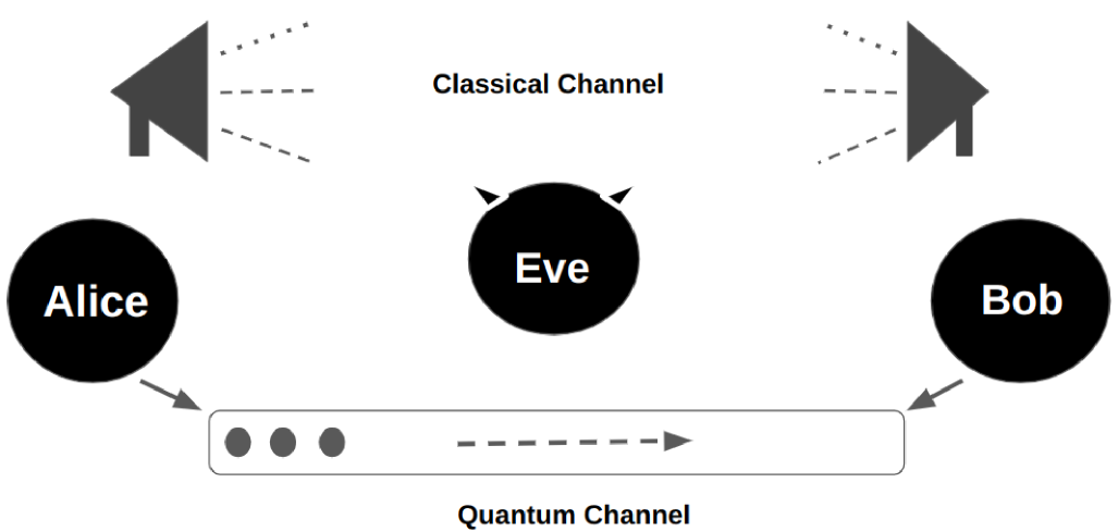
Figure 1: QSDC protocol.

II.2 Dynamics of open quantum systems

In contrast to isolated systems which undergo unitary evolution, the general quantum evolution of an open system can be described by a mathematical construct known as a Completely Positive Trace-Preserving (CPTP) map denoted as $\varepsilon(t_{\text{fin}},t_{\text{ini}})$. This CPTP map functions as a transformation operator, mapping an initial density operator $\rho(t_{\text{ini}})$ from the set of density operators $(\mathcal{D}(\mathcal{H}))$ to a final density operator $\rho(t_{\text{fin}})$ within the same set. Importantly, we assume that an inverse operation, denoted as $\varepsilon^{-1}(t_{\text{fin}},t_{\text{ini}})$, exists and is well-defined for all times ranging from $t_{\text{ini}}$ to $t_{\text{fin}}$. Consequently, we can express the dynamical evolution for any time interval $t_{\text{fin}}\geq t_{\text{int}}\geq t_{\text{ini}}$ as a composition,

$$\varepsilon_{(t_{fin},t_{ini})}=\varepsilon_{(t_{fin},t_{int})}\circ\varepsilon_{(t_{int},t_{ini})}$$ (1)

The map $\varepsilon_{(t_{\text{fin}},t_{\text{ini}})}$ is always completely positive as it represents a physical process. The map $\varepsilon_{(t_{\text{int}},t_{\text{ini}})}$ is also completely positive due to the lack of interaction with the environment. However, $\varepsilon_{(t_{\text{fin}},t_{\text{int}})}$ may not always be completely positive. A quantum dynamics applied to a system is considered divisible if it can be expressed in the form of equation (1) for any time interval $t_{\text{fin}}\geq t_{\text{int}}\geq t_{\text{ini}}$. Here, $t_{\text{ini}}$ denotes the initial time of the dynamics, and the symbol $\circ$ signifies the composition of two maps.

This dynamics, denoted as $\varepsilon(t_{\text{fin}},t_{\text{ini}})$, is termed positive divisible (P-divisible) when the map $\varepsilon(t_{\text{fin}},t_{\text{int}})$ is positive for every $t_{\text{fin}}\geq t_{\text{int}}\geq t_{\text{ini}}$, satisfying the prescribed composition law. Likewise, the dynamics is termed completely positive divisible (CP-divisible) when the map $\varepsilon(t_{\text{fin}},t_{\text{int}})$ is a Completely Positive Trace-Preserving (CPTP) map for every $t_{\text{fin}}\geq t_{\text{int}}\geq t_{\text{ini}}$, while adhering to the composition law.

The mathematical representation of a dynamical map $\varepsilon(t_{\text{fin}},t_{\text{ini}})$ in terms of “divisibility”, where we describe memoryless evolution as a composition of physical maps, plays a pivotal role in defining the concept of quantum Markovianity. According to the RHP criterion PhysRevLett.105.050403 , a dynamics is deemed non-Markovian if it fails to exhibit Complete Positive Divisibility (CP-divisibility). An alternative approach to characterizing non-Markovian dynamics, as proposed by Breuer et al. PhysRevLett.103.210401 ; PhysRevA.81.062115 , focuses on the distinguishability of quantum states after undergoing the action of a dynamical map. When a quantum system interacts with a noisy environment, the distinguishability between two quantum states gradually diminishes over time due to this interaction. However, if, at any given moment, the distinguishability of quantum states increases, it signifies a reverse flow of information from the environment back to the quantum system. This phenomenon serves as a clear indicator of non-Markovianity.

The former method of identifying non-Markovian dynamics is referred to as “RHP-type non-Markovianity” PhysRevLett.105.050403 ; rivas2014quantum , while the latter is known as “BLP-type non-Markovianity” PhysRevLett.103.210401 ; RevModPhys.88.021002 . It’s important to note that a dynamics considered Markovian in the RHP sense will also be Markovian in the BLP sense. However, the reverse is not necessarily true in all cases. Hence, while the breaking of CP divisibility is a necessary condition, it is not always sufficient to conclude that there is information backflow from the environment to the quantum system.

II.3 Non-Markovian Quantum channels

We will briefly explore some non-Markovian models, which are later employed to analyze the effectiveness of the DI-QSDC protocol. These models describe the behavior of a system as it interacts with its environment, and this interaction is mathematically represented using Kraus operators.

$$\varepsilon(\rho)=\sum_{i=1}^{n}E_{i}(t)\rho E_{i}^{\dagger}(t)$$ (2)

In this context, we apply this method to characterize dissipative amplitude damping and pure dephasing interactions in the presence of non-Markovian environments. The Kraus operators that represent P-indivisible amplitude damping noise within the framework of non-Markovian effects bellomo2007non on qubit systems can be expressed as follows:

$$E_{0}^{AD}=\ket{0}\bra{0}+\sqrt{p(t)}\ket{1}\bra{1}\text{,}\;\;E_{1}^{AD}=\sqrt{{1-p(t)}}\ket{0}\bra{1}$$ (3)

where the function $p(t)$ is defined as $\exp{-\Gamma t}[\cos(b\frac{t}{2})+\frac{\Gamma}{b}\sin(b\frac{t}{2})]^{2}$, with $b=\sqrt{(2\gamma\Gamma-\Gamma^{2})}$. In these expressions, $\Gamma$ represents the linewidth, which is intricately linked to the reservoir’s correlation time $\Gamma\approx\tau_{B}^{-1}$, while $\gamma$ signifies the coupling strength associated with the relaxation time of the qubit $\gamma\approx\tau_{R}^{-1}$. When the reservoir correlation time significantly exceeds the qubit relaxation time, we observe the emergence of memory effects. These effects are indicative of the non-Markovian nature of dissipation. Consequently, the relationship defined by $2\gamma/\Gamma$ dictates whether the noise displays Markovian characteristics when $2\gamma\leq\Gamma$ or non-Markovian behavior otherwise.

In a similar fashion, a Kraus operator for the P-divisible dephasing channel can be expresed as utagi2020temporal .

$$E_{0}^{D_{ph}}=\ket{0}\bra{0}+p(t)\ket{1}\bra{1}\text{,}\;\;E_{1}^{D_{ph}}=\sqrt{{1-p^{2}(t)}}\ket{1}\bra{1}$$ (4)

Here, the function $p(t)$ is defined as $\text{exp}[-\frac{\gamma}{2}\{t+\frac{1}{\Gamma}(\text{exp}(-\Gamma t)-1)\}]$. As the linewidth $\Gamma$ tends towards infinity, the dephasing channel makes a transition towards the Markovian case.

III DI-QSDC protocol under environmental noise

The DI-QSDC protocol is based on two fundamental assumptions, first, unwanted information from Alice and Bob’s physical surroundings may escape to the outer world. The second is that quantum physics is true. As shown in fig-(2) the QSDC protocol is described in five stages:

Stage:1 This stage is the state generation part, where Alice prepares N number of EPR pairs in her laboratory. The checking (C) photon sequence and the message (M) photon sequence, are the two photon sequences into which she separates the N, EPR pairs. However, She will randomly tag the prepared EPR pairs as check or message pair.

Stage 2: In this stage Alice uses the quantum non-Markovian channel to deliver Bob the photons in the C sequence one at a time. This process is called the first photon transmission. The single photon could lose its entire signal during transmission because of environmental noise and channel loss. The total photon transmission efficiency ($\eta$) directly depends upon the communication length between Alice and Bob ($D_{AB}$), which can be written as scaraniV

$$\eta=10^{-\frac{\alpha D_{AB}}{10}}$$ (5)

where $\alpha$ is the attenuation factor. After the effect of decoherence, the initial state, $\rho_{0}=|\phi^{+}\rangle\langle\phi^{+}|$ written as,

$$\rho_{AB}=\sum_{i}(\mathbb{I}\otimes E_{i})\rho_{0}(\mathbb{I}\otimes E^{\dagger}_{i})$$ (6)

where, $E_{i}$ are the Kraus operators defined in equation (3) or equation (4), which satisfy $\sum_{i}E^{\dagger}_{i}E_{i}=\mathbb{I}$. When both photon transmission loss and decoherence is considered, the N shared states between Alice and Bob become

$$\rho_{1}=\eta\rho_{AB}+(1-\eta)\mathbb{I}/4$$ (7)

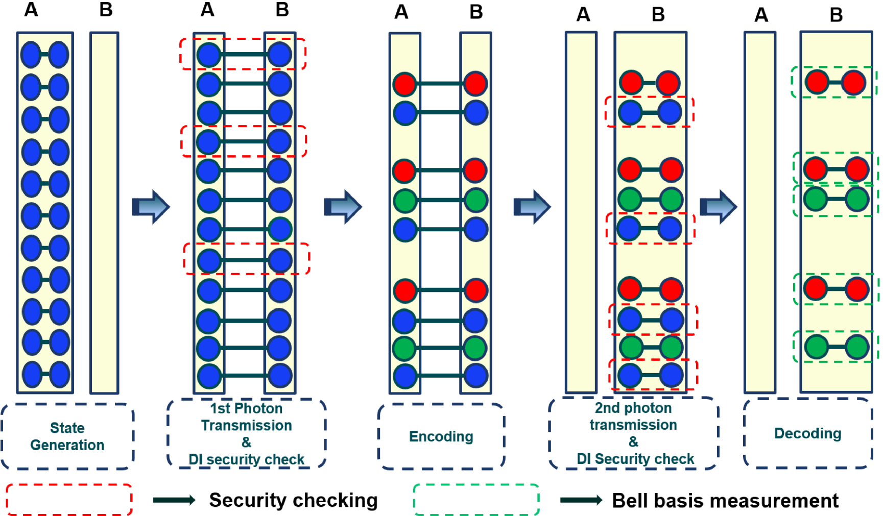
Figure 2: Schematic diagram for QSDC protocol (Red colour entangled pair photons are $\ket{\psi^{+}}$, green colour entangled pair photons are $\ket{\psi^{-}}$ and blue colour entangled pair photons are $\ket{\phi^{+}}$).

In this second stage, Alice and Bob also do the initial security checks to guarantee the safety of the first photon transmission operation. Alice first randomly chooses a large enough group of photons from the C photon sequence to perform the security check before revealing their positions to Bob over the public channel. Alice and Bob individually perform some measurements on each of the security-checking photons (C) photon sequence. Alice has four possible binary measurements bases $A_{0}=\sigma_{x}$, $A_{1}=\frac{(\sigma_{z}+\sigma_{x})}{\sqrt{2}}$, $A_{2}=\frac{(\sigma_{z}-\sigma_{x})}{\sqrt{2}},$ and $A_{3}=\sigma_{z}$ with binary outcomes $a_{i}\in\{-1,+1\}$ and Bob has two possible measurement $B_{0}=A_{0}$ and $B_{1}=A_{3}$ with binary outcomes $b_{j}\in\{-1,+1\}$. Once all of the checking photon pairs have been measured, Alice and Bob broadcast their measurement basis and results over a public channel. There are four possibilities.
Case 1:If Alice choose $A_{1}$ or $A_{2}$ measurement bases then they can estimate the CHSH functional

$$S_{l}=\langle a_{1}b_{1}\rangle+\langle a_{1}b_{2}\rangle+\langle a_{2}b_{1}\rangle-\langle a_{2}b_{2}\rangle$$ (8)

where $l=1,2;$ for first and second round photon transmission respectively and $\langle a_{i}b_{j}\rangle=[P(a_{i}=b_{j})-P(a_{i}\neq b_{j})]$. We make the assumption that all measurement margins are random without losing generality, such that $\langle a_{i}\rangle=0,\langle b_{j}\rangle=0$ for $i\in\{0,1,2,3\}$ and $j\in\{0,1\}$
Case 2: If Alice chooses measurement basis $A_{0}$ and Bob chooses measurement basis $B_{0}$ then the measurement result is used to estimate the quantum bit-flip error rate $Q_{b1}$ as

$$Q_{b1}=P(a_{0}\neq b_{0})$$ (9)

Case 3: If Alice choose measurement basis $A_{3}$ and Bob choose $B_{1}$, then the measurement result is used to estimate the quantum phase-flip error rate $Q_{p1}$ as

$$Q_{p1}=P(a_{3}\neq b_{1})$$ (10)

In this work, we are interested in the total QBER,

$$Q_{l}=Q_{bl}+Q_{pl}.$$ (11)

where $l=1,2;$ for first and second round photon transmission respectively.
Case 4: The measurement results obtained when Alice choose $A_{0}$ and Bob choose $B_{1}$, or when Alice choose $A_{3}$ and Bob choose $B_{0}$, are ignored or removed from the remaining analysis.

If the CHSH functional, $S_{1}\leq 2$ then Alice and Bob are classically correlated. Since the first photon-transmission method is insecure in this scenario, the parties must terminate their communication because Eve might intercept the photons without being noticed. If the CHSH functional, $S_{1}>2$ then Alice and Bob are non-locally correlated. In this case the rate at which Eve intercepts the photons is limited. After making sure that the initial photon transfer is secure, Alice and Bob go on to the subsequent step.

Stage 3: This is the enoding part, where Alice retrieves the photons that were saved from the memory storage. She uses one of the two unitary procedures to encrypt her messages onto the message photon sequence (M). The two unitary operations are

$$U_{0}=\sigma_{x},U_{1}=i\sigma_{y}$$ (12)

Alice is able to change the state of the system from $|\phi^{+}\rangle$ to $|\psi^{+}\rangle$ and $|\psi^{-}\rangle$ using the unitary operations $U_{0}$ and $U_{1}$ respectively. Alice can encrypt her messages ”0” and ”1” onto the photon pairs by applying $U_{0}$ and $U_{1}$ respectively.

Stage 4: In the second photon transmission round, Alice chooses a few photons at random to serve as security check photons and she does not apply any operation on them. Alice deliberately shuffles the order of her photons in sequence and records the initial positions of each photon to prevent Eve from precisely intercepting the encoded photons based on her interceptions during the first round. Alice transmits all the photons from the sequence to Bob and publicly discloses the locations of each photon in the initial sequence after the transmission. Subsequently, Bob successfully reconstructs the original sequence. The second phase of security checking is subsequently carried out by Bob using Alice’s announcement of the locations of the security checking photons.

The decoherence and the 2nd photon transmission loss influence the security-checking photon states on Bob’s side. The security-checking photon state becomes

$$\rho_{2}=\eta\tilde{\rho}_{AB}+(1-\eta)\mathbb{I}/4$$ (13)

The state $\rho_{1}$ transforms to another mixed noisy state say, $\tilde{\rho}_{AB}(=\sum_{i}(E_{i}\otimes\mathbb{I})\rho_{1}(E^{\dagger}_{i}\otimes\mathbb{I}))$, due to transmission through the noisy channel.

After the measurements procedures, Bob can estimate the CHSH functional $S_{2}$ and calculate the $Q_{b2}$ and $Q_{p_{2}}$. If the second photon-transmission procedure is not secure when $S_{2}\leq 2$, the parties abandon the communication. Otherwise, if the functional $S_{2}>2$ they ensure that the photon transmission is secure and go to the subsequent step. It may be noted here that after the 2nd photon transmission, the CHSH function $S_{1}>S_{2}$ always.

Stage 5: In this final stage, Bob decodes the encrypted messages. For this, he performs the Bell basis measurements on all the remaining photons, and based on the measurements he is able to distinguish between $|\psi^{+}\rangle$ and $|\psi^{-}\rangle$, where the initial entangled state is $|\phi^{+}\rangle$.

At the end of the protocol, Alice and Bob calculate the secret message capacity and the maximum distance for which they can send the secret message.

In this device-independent scenario, we make a general assumption that Eve obeys the laws of quantum physics. Furthermore, it is assumed that the measurement findings received by each side are entirely dependent on their present inputs. Here we consider a collective attack in which Eve applies an identical attack against each of Alice’s and Bob’s systems. In this way, all the photon pairs have the same form after transmission. The ability to send secret messages $C_{s}$ is defined as the ratio of successfully and securely transferred qubits to the total number encoded photon pairs. In scenarios involving non-ideal devices and noisy channels, the minimum achievable capacity for securely transmitting a secret message from Alice to Bob, considering collective attacks, is bounded below by the Devetak-Winter rate.DW05 ,

$$C_{s}\geq I(A:B)-I(A:E)$$ (14)

where, $I(A:B)$ and $I(A:E)$ are the mutual information between Alice and Bob, and mutual information between Alice and Eve respectively. It is assumed that mutual information between Alice and Bob is uniformly marginally distributed, as Acin07 ; sp09

$$I(A:B)=1-h(Q_{2})$$ (15)

where $Q_{2}$ $(=Q_{b2}+Q_{p2}$) is the total quantum bit error rate (QBER) after the 2nd photon transmission, and $h(p)$ is the binary entropy defined as,

$$h(p)=-p\log_{2}p-(1-p)\log_{2}(1-p)$$ (16)

After the first and second rounds of photon transmission, we can estimate the Holevo quantities, given by

$$\chi(S_{1})\leq h\left(\frac{1+\sqrt{(S_{1}/2)^{2}-1}}{2}\right)$$

$$\chi(S_{2})\leq h\left(\frac{1+\sqrt{(S_{2}/2)^{2}-1}}{2}\right)$$ (17)

Comparing the Bell-CHSH functionals of the 1st round and 2nd round photon transmissions, one has $S_{1}>S_{2}$, and hence, it follows that the Holevo quantities must obey $\chi(S_{1})<\chi(S_{2})$.

Here the mutual information between Alice and Eve $I(A:E)$ is denoted as the message intercepting rate, which is bounded by the Holevo quantity Hol73

$$I(A:E)\leq\chi(S_{1})$$ (18)

$I(A:E)$ can reach the maximum value of $\chi(S_{1})$ only if, during the second round of photon transmission, Eve manages to intercept all the photons corresponding to those she intercepted in the initial photon transmission. However, since Alice reshuffles the sequence of her photons before the second transmission, the probability of $I(A:E)$ reaching $\chi(S_{1})$ diminishes significantly, particularly with a substantial number of transmitted photons.

Using the equations (15), (III) and (18) we can find the lower bound of $C_{s}$ to be

$$C_{s}\geq 1-h(Q_{2})-\chi(S_{1})$$ (19)

By incorporating the Kraus operators from equation (3) into the expressions given by equations (7) and (13), we can determine the Bell-CHSH functional, denoted as $S_{1}$ and $S_{2}$ repectively, for both the photon transmissions. In the case of an amplitude damping channel, they are given by

$$S_{1}=\bigl{(}1+\sqrt{p(t)}\bigr{)}\eta\sqrt{2p(t)}$$ (20)

$$S_{2}=\bigl{(}1-p(t)+2p^{2}(t)\bigr{)}\eta^{2}\sqrt{2}$$ (21)

Likewise, by applying the Kraus operators from equation (4), $S_{1}$ and $S_{2}$, for the dephasing channel are given by

$$S_{1}=\bigl{(}1+p(t)\bigr{)}\eta\sqrt{2}$$ (22)

$$S_{2}=\bigl{(}1+p^{2}(t)\bigr{)}\eta^{2}\sqrt{2}$$ (23)

Next, using equations (7) and (13) we can determine the total QBER in equation (11). $Q_{1}$ and $Q_{2}$ in the context of an amplitude damping channel are given by

$$Q_{1}=1-\frac{\eta\sqrt{p(t)}}{2}\bigl{(}1+\sqrt{p(t)}\bigr{)}$$ (24)

$$Q_{2}=1-\frac{\eta^{2}}{2}\bigl{(}1-p(t)+2p^{2}(t)\bigr{)}$$ (25)

Similarly, the total QBER in case of the dephasing channel is given by

$$Q_{1}=1-\frac{\eta}{2}\bigl{(}1+p(t)\bigr{)}$$ (26)

$$Q_{2}=1-\frac{\eta^{2}}{2}\bigr{(}1+p^{2}(t)\bigl{)}$$ (27)

Now, from equations (16), (III), we get the secret message capacity $C_{s}$ under the amplitude damping channel, as

$$C_{s} =\Omega\log_{2}(\Omega)+(1-\Omega)\log_{2}(1-\Omega)$$

$$+\frac{1-\delta}{2}\log_{2}(1-\delta)+\frac{1+\delta}{2}\log_{2}(1+\delta)$$ (28)

where, $\Omega=\frac{\eta^{2}}{2}(1-p(t)+2p^{2}(t))$, and $\delta=\sqrt{\frac{\eta^{2}p(t)}{2}(1+\sqrt{p(t)})^{2}-1}$.

Similarly, for dephasing channel, we compute the secret message capacity to be,

$$C_{s} =\omega\log_{2}(\omega)+(1-\omega)\log_{2}(1-\omega)$$

$$+\frac{1-\Delta}{2}\log_{2}(1-\Delta)+\frac{1+\Delta}{2}\log_{2}(1+\Delta)$$ (29)

Where, $\omega=\frac{\eta^{2}}{2}(1+p^{2}(t))$, and $\Delta=\sqrt{\frac{\eta^{2}}{2}(1+p(t))^{2}-1}$.

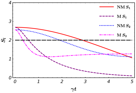
(a) The Bell-CHSH functional ($\boldsymbol{S_{l}}$) (where $\boldsymbol{l}=1,2$ for first and second photon transmission respectively) is plotted against Noise parameter ($\boldsymbol{\gamma t}$) for Markovian (M) ($\Gamma=5\gamma$) and non-Markovian (NM) ($\Gamma=0.1\gamma$) amplitude damping channel (here $\eta=0.95$).

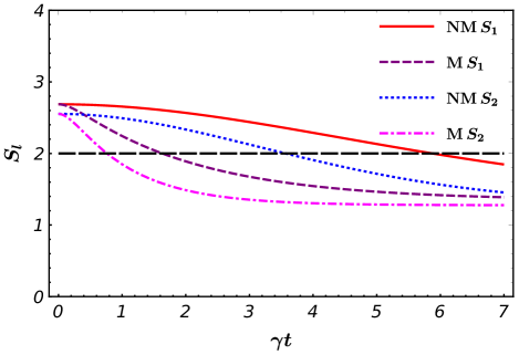
(b) The Bell-CHSH functional ($\boldsymbol{S_{l}}$) (where $\boldsymbol{l}=1,2$ for first and second photon transmission respectively) is plotted against Noise parameter ($\boldsymbol{\gamma t}$) for Markovian (M) ($\Gamma=5\gamma$) and non-Markovian (NM) ($\Gamma=0.1\gamma$) dephasing channel (here $\eta=0.95$).

Figure 3: The Bell-CHSH functional (for both round photon transmissions) is plotted against the noise parameter ($\boldsymbol{\gamma t}$) for the amplitude damping and dephasing channels for the Markovian and non-Markovian regions.

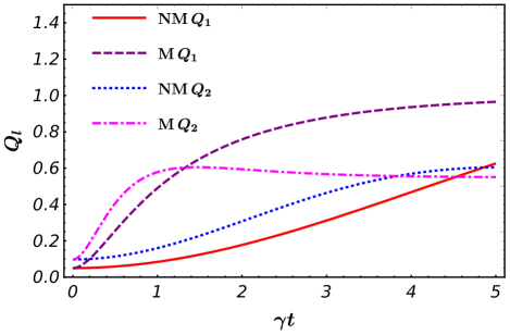
(a) The QBER ($\boldsymbol{Q_{l}}$) (where $\boldsymbol{l}=1,2$ for first and second photon transmission respectively) is plotted against Noise parameter ($\boldsymbol{\gamma t}$) for Markovian (M) ($\Gamma=5\gamma$) and non-Markovian (NM) ($\Gamma=0.1\gamma$) amplitude damping channel (here $\eta=0.95$).

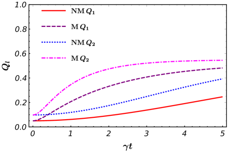
(b) The QBER ($\boldsymbol{Q_{l}}$) (where $\boldsymbol{l}=1,2$ for first and second photon transmission respectively) is plotted against Noise parameter ($\boldsymbol{\gamma t}$) for Markovian (M) ($\Gamma=5\gamma$) and non-Markovian (NM) ($\Gamma=0.1\gamma$) dephasing channel (here $\eta=0.95$).

Figure 4: The quantum bit error rate (QBER) (for both round photon transmissions) is plotted against the noise parameter ($\boldsymbol{\gamma t}$) for the amplitude damping and dephasing channels for the Markovian and non-Markovian regions.

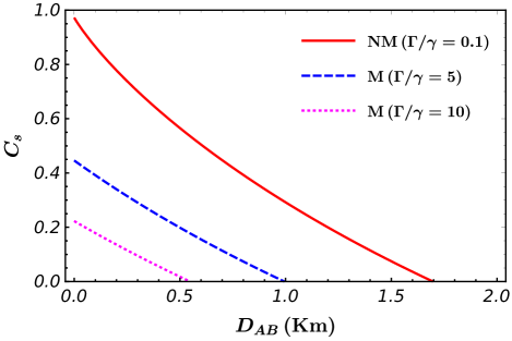
(a) The secret message capacity ($\boldsymbol{C_{s}}$) is plotted against Communication length ($\boldsymbol{D_{AB}}$ (Km)) for Markovian (M) ($\Gamma/\gamma=5,10$) and Non-Markovian (NM) ($\Gamma/\gamma=0.1$) amplitude damping channel for $\gamma t=0.15$.

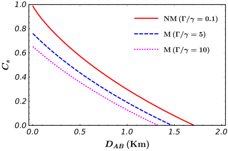
(b) The secret message capacity ($\boldsymbol{C_{s}}$) is plotted against Communication length ($\boldsymbol{D_{AB}}$ (Km)) for Markovian (M) ($\Gamma/\gamma=5,10$) and Non-Markovian (NM) ($\Gamma/\gamma=0.1$) dephasing channel for $\gamma t=0.15$.

Figure 5: The secret message capacity ($\boldsymbol{C_{s}}$) is plotted against communication length ($\boldsymbol{D_{AB}}$ (Km)) for amplitude damping and dephasing channels for the Markovian and non-Markovian regions.

In the following section we compute the above three key performance indicators of the DI-QSDC protocol, namely, the communication capacity, the quantum bit error rate and the Bell-CHSH functional under the action of Markovian and non-Markovian amplitude damping as well as dephasing noise channels choosing values of parameters in an experimentally realizable range tang2012 ; passos2019 .

IV Effect of non-markovian channels

In this section, we discuss the dynamical behaviour of the benchmark physical parameters when the DI-QSDC task is performed between Alice and Bob under the action of a noisy channel, and under attack by a eavesdropper. In order to evaluate the effect of non-Markovian dynamics, the ratio $\Gamma/\gamma$ plays the most significant role. For instance, transitions between the Markovian and non-Markovian regimes have been realized in cavity quantum electrodynamics experimental configurations kuhr2007ultrahigh using Rydberg atoms with a lifetime of $\tau_{\text{at}}=30$ ms, with a cavity lifetime of $\tau_{\text{cav}}=130$ ms. The single photon’s relaxation time in a superconducting cavity is $25.6\pm 0.2$. msmilul2023superconducting . In our subsequent calculations, the ratio of the $\gamma$ and $\Gamma$ parameters are chosen to lie within the experimentally feasible range of all optical set-ups tang2012 ; passos2019 . Additionally, we take the attenuation factor to be $\alpha=0.2$ dB/Km, which corresponds to a transmission efficiency $\eta\approx 95\%$ for a communication distance of the order of $1$ Km zapatero2019 .

Let us first consider the stage 2, when Alice and Bob perform the DI security checking task after the first photon transmission. In fig(3(a)) we show the dynamics of the Bell-CHSH functionals ($S_{1}$, $S_{2}$) against the noise parameter $\gamma t$. Here we consider the amplitude damping channel. It can be seen that we get a larger non-classical region (up to $\gamma t$ = 3 (red)) under non-Markovian dynamics compared to the non-classical region (up to $\gamma t$= 0.6 (purple)) under Markovian dynamics. We next consider stage 4, when the second DI security checking task is performed after the second photon transmission. In this case too, compared to a Markovian regime (up to $\gamma t$ = 0.4 (magenta)), a non-Markovian regime (up to $\gamma t$ = 2 (blue)) corresponds to a bigger non-classical region.
A similar behaviour is exhibited for the dephasing channel. As seen from fig.(3(b)) when the dephasing channel is taken into account, here too we get a larger non-classical region in non-Markovian regime (up to $\gamma t$ = 5.8 (red) and 3.6 (blue)) compared to the Markovian regime (up to $\gamma t$ = 1.6 (purple) and 0.8 (magenta) after the 1st and 2nd photon transmission, respectively) in the behaviour of the Bell-CHSH functionals ($S_{1}$, $S_{2}$).
It is worthwhile to note that for the same value of the noise parameter $\gamma$, a non-Markovian channel leads to a higher value of the Bell-CHSH parameter, signifying an enhanced level of security compared to a Markovian channel. Comparing fig.(3(a)) and fig.(3(b)), it may be noted further that the dephasing channel enables the achievement of a bigger non-classical region compared to the case of the amplitude damping channel, a result that is valid irrespective of the Markovian or non-Markovian nature of the dynamics.

We next analyze the behaviour of the quantum bit error rate under the various dynamics considered here. In figs(4(a), 4(b)) where we plot total QBER ($Q_{1}$, $Q_{2}$) (after the first and second photon transmissions, respectively) against the noise parameter $\gamma t$. It can be seen that we get less QBER in the non-Markovian regime compared to the Markovian regime under both amplitude and dephasing noise. Thus, action of a non-Markovian channel leads to lesser error rate than that under action of a Markovian channel for both the amplitude damping and the dephasing noise. Further, a comparison of the fig.(4(a)) and fig.(4(b)) exhibits less QBER value under dephasing noise. One can see that QBER values can be more than $0.8$ under amplitude damping noise, but it does not exceed the value of $0.5$ when we consider dephasing noise. So, it turns out that as with the case of the Bell-CHSH functional, a dephasing channel turns out to be a better option for our DI-QSDC protocol compared to an amplitude damping channel for either Markovian or non-Markovian dynamics.

We finally investigate the secret message capacity $C_{s}$. From fig.(5(a)) in case of amplitude damping channel, we can observe that the secret message can be communicated over a maximum communication distance of $D_{AB}=1.7$ km (red) in the non-Markovian regime. This gives an advantage over the Markovian channel, where we can communicate only up to $D_{AB}=0.55$ km (magenta) for $\Gamma/\gamma=10$. After increasing the strength of the parameter but still confining to the Markovian regime, one sees that $D_{AB}$ increases to 1 km (blue). Further, one can see that the the secret message capacity can be maximum, i.e. almost $1$, in the non-Markovian regime for very short distances, while in the Markovian regime it is considerably lesser.

In fig.(5(b)) we display the secret message capacity under the action of dephasing noise. Here too the advantage under non-Markovian dynamics is exhibited, corresponding to a larger communication distance compared to the case of Markovian dynamics. Similarly again, secret message capacity at short distances is considerably larger under non-Markovian dynamics. If we compare the maximum communication under non-Markovian channels for the amplitude damping with the dephasing channel (comparing fig.(5(a)) and fig.(5(b)), it is observed that both turn out to be nearly the same. In contrast, the maximum communication length is larger for the dephasing noise undergoing Markovian dynamics compared to the amplitude damping dynamics.

V Conclusions

Quantum cryptography is a rapidly developing sector under quantum technologies. The advancement in the single photon sources and detectors have accelerated interest in quantum key distribution products. However, three primary challenges needs to be addressed: (i) decoherence due to interaction with the channel noise, (ii) device imperfections and implementation loopholes, and (iii) security challenges such as authentication, key management and key migration. In this regard, device independent quantum communication tasks have been proposed that somewhat address the issues (ii) and (iii). Considerable further effort is required to address the issue (i).

With the above motivation in the present work, we analyse the performance of device-independent quantum secure direct communication under non-Markovian noise modelled by amplitude damping and dephasing quantum channels. Here we have performed a detailed analysis on the effect of non-Markovian noise on the efficacy of the DI-QSDC task when both the entangled photons interact with the decohering quantum channel one at a time during their transit in the DI-QSDC protocol. We have investigated the role of non-Markovian noise in Bell-inequality violation, quantum bit error rate (QBER), and communication capacity.

Our results show that non-Markovian environmental dynamics leads to enhanced Bell-violation, decrease in the qubit error rate, as well as increase in the communication capacity. Improvement of performace of the DI-QSDC protocol is thus displayed with regard to all these three benchmark parameters for both in the case of non-Markovian amplitude damping as well as non-Markovian dephasing quantum channels. Our present analysis should motivate further theoretical studies on different quantum communication protocols under realistic environmental scenarios modeled by Markovian and non-Markovian noisy channels, and also experimental reservoir engineering protocols aimed towards driving open systems from the Markovian to the non-Markovian regime nphys2011 ; wang2018 .

Acknowledgements: SB and ASM acknowledge support from the Project No. DST/ICPS/QuEST/2018/98 from the Department of Science and Technology, Government of India. SG acknowledges the support from QuNu Labs Pvt Ltd and OIST, Japan.

References

- (1) Rivest, R. L., Shamir, A. and Adleman, L., A method for obtaining digital signatures and public-key cryptosystems, Commun. ACM 21, 120–126 (1978)
- (2) Shor, PW, Algorithms for quantum computation: discrete logarithms and factoring, Proceedings 35th Annual Symposium on Foundations of Computer Science, Santa Fe, NM, USA, 1994, pp. 124-134
- (3) Lov K. Grover, A fast quantum mechanical algorithm for database search, arXiv:quant-ph/9605043 (1996)
- (4) Long, G. L., Grover algorithm with zero theoretical failure rate, Phys. Rev. A 64, 022307 (2001)
- (5) Nicolas Gisin, Grégoire Ribordy, Wolfgang Tittel, and Hugo Zbinden, Quantum cryptography, Rev. Mod. Phys. 74, 145 (2002).
- (6) C. H. Bennett et al. Teleporting an unknown quantum state via dual classic and Einstein-Podolsky-Rosen channels., Phys. Rev. Lett. 70, 1895–1899 (1993).
- (7) C. H. Bennett, Quantum cryptography using any two nonorthogonal states, Phys. Rev. Lett. 68, 3121 (1992).
- (8) C. H. Bennett and G. Brassard, Quantum cryptography, public key distribution and coin tossing, Theoretical Computer Science, Vol. 560 (Part 1), pp. 7-11 (2014).
- (9) A. K. Ekert, Quantum cryptography based on Bell’s theorem , Phys. Rev. Lett. 67, 661 (1991).
- (10) Long GL, Liu XS. , Theoretically efficient high-capacity quantum-key- distribution scheme, Phys. Rev. A 65, 032302 (2002).
- (11) Hillery M, Bužek V, Berthiaume A. , Quantum secret sharing, Phys. Rev. A 59, 1829 (1999).
- (12) C.L. Degen, F. Reinhard, and P. Cappellaro, Quantum sensing, Rev. Mod. Phys. 89, 035002 (2017).
- (13) R. Horodecki, P. Horodecki, M. Horodecki, and K. Horodecki, Quantum entanglement, Rev. Mod. Phys 81, 865 (2009).
- (14) Roope Uola, Ana C.S. Costa, H. Chau Nguyen, and Otfried Guhne, Quantum steering, Rev. Mod. Phys. 92, 015001 (2020).
- (15) Nicolas Brunner, Daniel Cavalcanti, Stefano Pironio, Valerio Scarani, and Stephanie Wehner, Bell nonlocality, Rev. Mod. Phys. 86, 419 (2014).
- (16) M. D. Eisaman; J. Fan; A. Migdall; S. V. Polyakov, Invited Review Article: Single-photon sources and detectors, Rev. Sci. Instrum. 82, 071101 (2011).
- (17) A. Acín, N. Brunner, N. Gisin, S. Massar, S. Pironio, and V. Scarani, Device-Independent Security of Quantum Cryptography against Collective Attacks, Phys. Rev. Lett. 98, 230501 (2007).
- (18) M. Pawłowski, Security proof for cryptographic protocols based only on the monogamy of Bell’s inequality violations, Phys. Rev. A 82, 032313 (2010).
- (19) T. Pramanik, M. Kaplan and A. S. Majumdar, Fine-grained Einstein-Podolsky-Rosen steering inequalities, Phys. Rev. A 90, 050305(R) (2014).
- (20) U. Vazirani, T. Vidick, Fully Device Independent Quantum Key Distribution, Phys. Rev. Lett. 113, 140501 (2014).
- (21) Imran Khan, Bettina Heim, Andreas Neuzner, and Christoph Marquardt, Satellite-based qkd, Opt. Photonics News 29, 26 (2018).
- (22) Tang, BY., Liu, B., Zhai, YP. et al., High-speed and Large-scale Privacy Amplification Scheme for Quantum Key Distribution., Sci Rep 9, 15733 (2019)
- (23) J. Kołodyński, A. Máttar, P. Skrzypczyk, E. Woodhead, D. Cavalcanti, K. Banaszek, and A. Acín, Device-independent quantum key distribution with single-photon sources , Quantum 4, 260 (2020).
- (24) M. Farkas, M. B. Juandó, K. Łukanowski, J. Kołodyński, and A. Acín, Bell Nonlocality Is Not Sufficient for the Security of Standard Device-Independent Quantum Key Distribution Protocols , Phys. Rev. Lett. 127, 050503 (2021).
- (25) J. Singh, S. Ghosh, Arvind, S. K.Goyal, Role of Bell-CHSH violation and local filtering in quantum key distribution, Physics Letters A, Volume 392, 127158, (2021).
- (26) D. P. Nadlinger, P. Drmota, B. C. Nichol, G. Araneda, D. Main, R. Srinivas, D. M. Lucas, C. J. Ballance, K. Ivanov, E. Y-Z. Tan, P. Sekatski, R. L. Urbanke, R. Renner, N. Sangouard, J-D. Bancal, Experimental quantum key distribution certified by Bell’s theorem , Nature volume 607, pages 682–686 (2022).
- (27) Yash Wath, Hariprasad M, Freya Shah, and Shashank Gupta, , Eavesdropping a Quantum Key Distribution network using sequential quantum unsharp measurement attacks, The European Physical Journal Plus volume 138, Article number: 54 (2023).
- (28) S. Bera, S. Gupta and A.S. Majumdar, Device-independent quantum key distribution using random quantum states, Quantum Inf Process 22, 109 (2023).
- (29) R. Takahashi, Y. Tanizawa and A. Dixon, A high-speed key management method for quantum key distribution network, Eleventh International Conference on Ubiquitous and Future Networks (ICUFN), Zagreb, Croatia, 2019, pp. 437-442.
- (30) W. K. Wootters and W. H. Zurek , A single quantum cannot be cloned, Nature volume 299, pages802–803 (1982).
- (31) Dong Pan, Zaisheng Lin, Jiawei Wu, Haoran Zhang, Zhen Sun, Dong Ruan, Liuguo Yin and Gui Lu LongExperimental free-space quantum secure direct communication and its security analysis., Photonics Res. 8, 1522–1531 (2020).
- (32) L. Zhou, Y. B. Sheng, G. L. Long, Device-independent quantum secure direct communication against collective attacks, Science Bulletin, Volume 65, Issue 1, (2020).
- (33) L. Zhou, Y. B. Sheng, One-step device-independent quantum secure direct communication, Sci. China Phys. Mech. Astron. 65, 250311 (2022).
- (34) L. Zhou, Bao-Wen Xu, Wei Zhong, and Yu-Bo Sheng, Device-Independent Quantum Secure Direct Communication with Single-Photon Sources, Phys. Rev. Applied 19, 014036 (2023)
- (35) W. Zhang, D. S. Ding, Y. B. Sheng, L. Zhou, B. S. Shi, and G. C. Guo, Quantum Secure Direct Communication with Quantum Memory, Phys. Rev. Lett. 118, 220501 (2017).
- (36) T. Metger, Y. Dulek, A. Coladangelo and R. A. Friedman, Device-independent quantum key distribution from computational assumptions , New J. Phys. 23 123021 (2021).
- (37) F. Xu, Y. Z. Zhang, Q. Zhang, J. Pan, Device-independent quantum key distribution with random post selection , Phys. Rev. Lett. 128, 110506 (2022).
- (38) A. Singh, K. Dev, H. Siljak, H. D. Joshi and M. Magarini, Quantum Internet—Applications, Functionalities, Enabling Technologies, Challenges, and Research Directions, IEEE Communications Surveys and Tutorials, vol. 23, no. 4, pp. 2218-2247, Fourthquarter 2021.
- (39) T. Yu and J. H. Eberly, Phys. Rev. Lett. 93, 140404 (2004); P.J. Dodd and J. J. Halliwell, Phys. Rev. A 69, 052105 (2004); T. Yu and J. H. Eberly, Phys. Rev. Lett. 97, 140403 (2006); M. P. Almeida, F. de Melo, M. Hor-Meyll, A. Salles, S. P. Walborn, P.H. S. Ribeiro and L. Davidovich, Science 316, 579 (2007); B. Bellomo, R. L. Franco, S. Maniscalco and G. Compagno, Phys. Rev. A 78, 060302(R) (2008); A. Salles, F. de Melo, M.P. Almeida, M. Hor-Meyll, S. P. Walborn, P.H. S. Ribeiro and L. Davidovich, Phys. Rev. A 78, 022322 (2008); T. Yu and J. H. Eberly, Science 323, 598 (2009).
- (40) P. Badziag, M. Horodecki, P. Horodecki, and R. Horodecki, Local environment can enhance fidelity of quantum teleportation, Phys. Rev. A 62, 012311 (2000).
- (41) S. Bandyopadhyay, Origin of noisy states whose teleportation fidelity can be enhanced through dissipation, Phys. Rev. A 65, 022302 (2002).
- (42) B. Ghosh, A. S. Majumdar, N. Nayak, Environment assisted entanglement enhancement, Phys. Rev. A 74, 052315 (2006).
- (43) Rivu Gupta, Shashank Gupta, Shiladitya Mal, Aditi Sen De, Performance of Dense Coding and Teleportation for Random States –Augmentation via Pre-processing, Phys. Rev. A 103, 032608 (2021).
- (44) R. L. Franco and Giuseppe Compagno, Lectures on General Quantum Correlations and their Applications, edited by F. F. Fanchini, D. O. S. Pinto, and G. Adesso (Springer, 2017).
- (45) L. Mazzola, S. Maniscalco, J. Piilo, K.-A. Suominen, and B. M. Garraway, Sudden death and sudden birth of entanglement in common structured reservoirs, Phys. Rev. A 79, 042302 (2009).
- (46) Rivu Gupta, Shashank Gupta, Shiladitya Mal, Aditi Sen De, Constructive Feedback of Non-Markovianity on Resources in Random Quantum States, Phys. Rev. A 105, 012424 (2022).
- (47) T. Pramanik and A. S. Majumdar, Improving the fidelity of teleportation through noisy channels using weak measurement, Phys. Lett. A 377, 3209 (2013).
- (48) S. Datta, S. Goswami, T. Pramanik, A. S. Majumdar, Preservation of a lower bound of quantum secret key rate in the presence of decoherence, Phys. Lett. A 381, 897 (2017).
- (49) Shashank Gupta, Shounak Datta, A. S. Majumdar, Preservation of quantum non-bilocal correlations in noisy entanglement-swapping experiments using weak measurements, Phys. Rev. A 98, 042322 (2018).
- (50) S. Goswami, S. Ghosh, A. S. Majumdar, Protecting quantum correlations in the presence of amplitude damping channel, Phys. A: Math. Theor. 54, 045302 (2021)..
- (51) E.-M. Laine, H.-P. Breuer, J. Piilo, Nonlocal memory effects allow perfect teleportation with mixed states, Scientific Reports 4, 4620 (2014).
- (52) A. Altherr and Y. Yang., Quantum Metrology for Non-Markovian Processes, Phys. Rev. Lett. 127, 060501 (2021).
- (53) S. Bhattacharya, B. Bhattacharya, A. S. Majumdar, Thermodynamic utility of non-Markovianity from the perspective of resource interconversion, J. Phys. A: Math. Theor. 53, 335301 (2020); S. Bhattacharya, B. Bhattacharya, A. S. Majumdar, Convex resource theory of non-Markovianity, J. Phys. A: Math. Theor. 54, 035302 (2020).
- (54) Bi-Heng Liu, Li Li, YunFeng Huang, Chuan-Feng Li, Guang-Can Guo, Elsi-Mari Laine , Heinz-Peter Breuer and Jyrki Piilo, Experimental control of the transition from Markovian to non-Markovian dynamics of open quantum systems, Nature Physics 7, 931 (2011).
- (55) Deng, F. G. and Long, G. L., Secure direct communication with a quantum one- time pad, Phys. Rev. A 69, 052319 (2004).
- (56) Deng, F. G., Long, G. L. and Liu, X. S., Two-step quantum direct communication protocol using the Einstein-Podolsky-Rosen pair block, Phys. Rev. A 68, 042317 (2003).
- (57) ‘Angel Rivas, Susana F. Huelga, Martin B. Plenio, Entanglement and Non-Markovianity of Quantum Evolutions , Phys. Rev. Lett. 105, 050403 (2010).
- (58) Heinz-Peter Breuer, Elsi-Mari Laine, Jyrki Piilo, Measure for the Degree of Non-Markovian Behavior of Quantum Processes in Open Systems , Phys. Rev. Lett. 103, 210401 (2009).
- (59) Elsi-Mari Laine, Jyrki Piilo, Heinz-Peter Breuer, Measure for the non-Markovianity of quantum processes, Phys. Rev. A 81, 062115 (2010).
- (60) Elsi-Mari Laine, Jyrki Piilo, Heinz-Peter Breuer, Quantum non-Markovianity: characterization, quantification and detection, Reports on Progress in Physics 81, 062115 (2014).
- (61) Heinz-Peter Breuer, Elsi-Mari Laine, Bassano Vacchini, Colloquium: Non-Markovian dynamics in open quantum systems , Rev. Mod. Phys. 88, 021002 (2016).
- (62) Bruno Bellomo, R Lo Franco, Giuseppe Compagno, Non-Markovian effects on the dynamics of entanglement , Phys. Rev. Lett. 99, 160502 (2007).
- (63) Shrikant Utagi, R Srikanth, Subhashish Banerjee, Temporal self-similarity of quantum dynamical maps as a concept of memorylessness , Scientific Reports s41598-020-72211-3 (2020).
- (64) V. Scarani, H. Bechmann-Pasquinucci, N. J. Cerf, M. Dusek, N. Lutkenhaus, and M. Peev The security of practical quantum key distribution , RevModPhys.81.1301 (2009).
- (65) Igor Devetak and Andreas Winter, Distillation of secret key and entanglement from quantum states, RoyalSociety.461 (2005).
- (66) Stefano Pironio and Antonio Acín and Nicolas Brunner and Nicolas Gisin and Serge Massar and Valerio Scarani, Device-independent quantum key distribution secure against collective attacks, Pironio2009 (2009).
- (67) A. S. Holevo, Bounds for the Quantity of Information Transmitted by a Quantum Communication Channel, Problemy Peredachi Informatsii (1973).
- (68) Jian-Shun Tang, Chuan-Feng Li, Yu-Long Li, Xu-Bo Zou, Guang-Can Guo, Heinz-Peter Breuer, Elsi-Mari Laine and Jyrki Piilo, Measuring non-Markovianity of processes with controllable system-environment interaction, EPL 97, 10002 (2012).
- (69) M. Passos, P. Obando, W. Balthazar, F. Paula, J. Huguenin, and M. Sarandy, Non-Markovianity through quantum coherence in an all-optical setup, Opt. Lett. 44, 2478-2481 (2019).
- (70) Stefan Kuhr, Sébastien Gleyzes, Christine Guerlin, Julien Bernu, U Busk Hoff, Samuel Deléglise, Stefano Osnaghi, Michel Brune, J-M Raimond, Serge Haroche and others Ultrahigh finesse Fabry-Pérot superconducting resonator, Applied Physics Letters 90, 16 (2007).
- (71) Ofir Milul, Barkay Guttel, Uri Goldblatt, Sergey Hazanov, Lalit M. Joshi, Daniel Chausovsky , Nitzan Kahn, Engin Çiftyürek, Fabien Lafont, and Serge Rosenblum Superconducting Cavity Qubit with Tens of Milliseconds Single-Photon Coherence Time, PRX QUANTUM 4, 030336 (2023).
- (72) V. Zaptero, M. Curty, Long-distance device-independent quantum key distribution, Scientific Reports 9, 17749 (2019).
- (73) Kai-Hung Wang, Shih-Hsuan Chen, Yu-Cheng Lin, and Che-Ming Li, Non-Markovianity of photon dynamics in a birefringent crystal, Phys. Rev. A 98, 043850 (2018).