Simulation-Based Inference of Surface Accumulation and Basal Melt Rates of an Antarctic Ice Shelf from Isochronal Layers
Abstract
The ice shelves buttressing the Antarctic ice sheet determine the rate of ice-discharge into the surrounding oceans. The geometry of ice shelves, and hence their buttressing strength, is determined by ice flow as well as by the local surface accumulation and basal melt rates, governed by atmospheric and oceanic conditions. Contemporary methods resolve one of these rates, but typically not both. Moreover, there is little information of how they changed in time. We present a new method to simultaneously infer the surface accumulation and basal melt rates averaged over decadal and centennial timescales. We infer the spatial dependence of these rates along flow line transects using internal stratigraphy observed by radars, using a kinematic forward model of internal stratigraphy. We solve the inverse problem using simulation-based inference (SBI). SBI performs Bayesian inference by training neural networks on simulations of the forward model to approximate the posterior distribution, allowing us to also quantify uncertainties over the inferred parameters. We demonstrate the validity of our method on a synthetic example, and apply it to Ekström Ice Shelf, Antarctica, for which newly acquired radar measurements are available. We obtain posterior distributions of surface accumulation and basal melt averaging over 42, 84, 146, and 188 years before 2022. Our results suggest stable atmospheric and oceanographic conditions over this period in this catchment of Antarctica. Use of observed internal stratigraphy can separate the effects of surface accumulation and basal melt, allowing them to be interpreted in a historical context of the last centuries and beyond.
JGR: Earth Surface
Machine Learning in Science, University of Tübingen and Tübingen AI Center, Germany Department of Geosciences, University of Tübingen, Germany Alfred-Wegener-Institut, Helmholtz-Zentrum für Polar und Meeresforschung, Bremerhaven, Germany Department of Geosciences, Universität Bremen, Germany Max Planck Institute for Intelligent Systems, Tübingen, Germany
1 Introduction
The majority of the Antarctic Ice Sheet is buttressed by floating ice shelves [Bindschadler \BOthers. (\APACyear2011)] which provide large contact areas for ice-ocean interactions. Approximately half of the ice shelves’ total mass loss is attributed to ocean-induced melting at the underside of ice shelves [Depoorter \BOthers. (\APACyear2013)], and its spatiotemporal variability imprints ice flow dynamics farther upstream [Reese \BOthers. (\APACyear2017), Gudmundsson \BOthers. (\APACyear2019)]. Consequently, ice flow and ocean models need to be coupled for future projections; frameworks [Goldberg \BOthers. (\APACyear2019), Gladstone \BOthers. (\APACyear2021)], parameterizations [Burgard \BOthers. (\APACyear2022), Goldberg \BBA Holland (\APACyear2022)], and benchmarks [Asay-Davis \BOthers. (\APACyear2016)] for this task have been developed. Similarly, the local snow accumulation is influenced by atmospheric conditions and is crucial in determining ice shelf thickness [Winkelmann \BOthers. (\APACyear2012)]. As a result, ice flow models are also coupled to climate models for future projections [Goelzer \BOthers. (\APACyear2016), Pattyn \BOthers. (\APACyear2017)]. It is crucial to confront ice flow models with observations to validate them and investigate their ability to explain observed phenomena. Here, we present a new method that infers surface accumulation and basal melt rates (collectively, the mass balance parameters) from the ice shelves’ internal stratigraphy, which can be routinely mapped by radio-echo sounding.
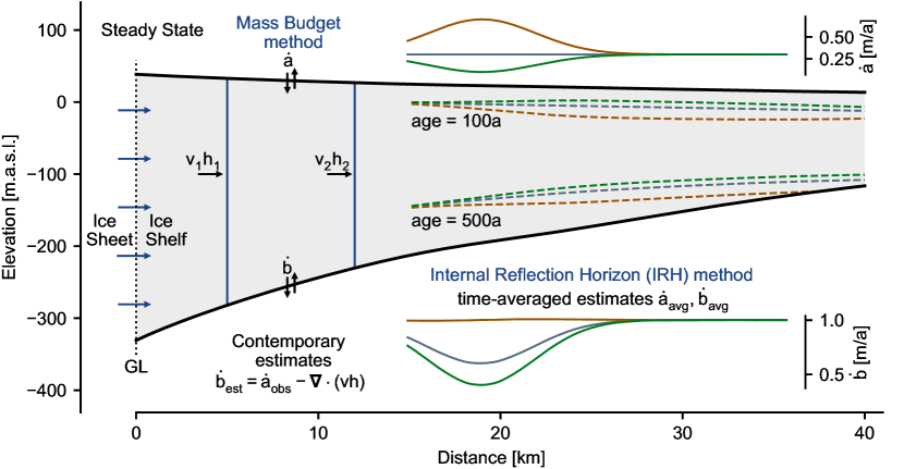
Previous studies provided much progress in deriving the mass balance parameters from observations. Typically, accumulation is more accessible [Eisen \BOthers. (\APACyear2008)]; it is measured in-situ using stake farms, and is also derived from multiple firn cores [Lenaerts \BOthers. (\APACyear2019)]. Many of these observations validate atmospheric models such as RACMO [van Wessem \BOthers. (\APACyear2018)] and MAR [Gallée \BBA Schayes (\APACyear1994), Agosta \BOthers. (\APACyear2019)], which estimate surface accumulation on 35 \unitkm grids [Lenaerts \BOthers. (\APACyear2019)] (with few locations being estimated at a higher resolution of 5.5 \unitkm). Estimating the basal melt is more challenging, and is typically dependent on knowledge of surface accumulation. For example, estimates of surface accumulation have been used along with mass conservation arguments to estimate basal melt [Neckel \BOthers. (\APACyear2012), Depoorter \BOthers. (\APACyear2013), Berger \BOthers. (\APACyear2017), Adusumilli \BOthers. (\APACyear2020)]. These approaches have provided Antarctic-wide time series of the last few decades of basal melt rates [Adusumilli \BOthers. (\APACyear2020)]. The spatial resolution is currently limited to the kilometer scale, which may miss fine grained processes occurring within ice shelf channels [Drews (\APACyear2015), Marsh \BOthers. (\APACyear2016)] or near basal terraces [Dutrieux \BOthers. (\APACyear2014)]. Independent estimates of basal melt are also available, but typically only on short temporal scales; for example, with time-lapse radar measurements of ice thickness change [Zeising \BOthers. (\APACyear2022)]. Using phase-coherent data acquisition, these measurements can disentangle the observed thickness change into strain thinning and basal melt [Nicholls \BOthers. (\APACyear2015)]. This has provided much insights, e.g., in terms of relevant tidal [Sun \BOthers. (\APACyear2019)] and seasonal timescales [Vaňková \BBA Nicholls (\APACyear2022)].
Here, we investigate to what extent the radar-imaged isochronal ice stratigraphy [Eisen \BOthers. (\APACyear2004)] can provide additional information for inferring mass balance parameters. On grounded ice, radar-imaged Internal Reflection Horizons (IRHs) have been used in multiple ways, for example to infer the surface accumulation history [Waddington \BOthers. (\APACyear2007), MacGregor \BOthers. (\APACyear2009), Catania \BOthers. (\APACyear2010), Steen-Larsen \BOthers. (\APACyear2010), Wolovick \BOthers. (\APACyear2021), Theofilopoulos \BBA Born (\APACyear2023)], velocity patterns of the ice flow [Eisen (\APACyear2008), Holschuh \BOthers. (\APACyear2017)], ice-rise evolution [Drews \BOthers. (\APACyear2015), Henry \BOthers. (\APACyear2023)], or large-scale model calibration [Sutter \BOthers. (\APACyear2021)]. On ice shelves, accumulation is also derived from the radar-measured shallow stratigraphy [Pratap \BOthers. (\APACyear2022)], but not from intermediate depths and below where the stratigraphy is also influenced by basal melt and ice flow. The stratigraphy of ice shelves differs for various combinations of surface accumulation and basal melt [Višnjević \BOthers. (\APACyear2022)]. This suggests that given an ice flow model of the internal stratigraphy that accounts for the mass balance parameters, we can use observed IRHs to recover the surface accumulation and basal melt histories (Fig. 1). Thus, our goal is to solve the inverse problem of inferring the surface accumulation and basal melt rates that can explain the observed IRHs under the physical constraints of the ice flow model.
Inverse problems, also known as inversion, data assimilation or inference problems in the literature, denote the task of finding the model parameters that are compatible both with empirical observations and prior knowledge. This problem is widespread in the geosciences, e.g. in hydrogeology [Linde \BOthers. (\APACyear2015)], seismology [Symes (\APACyear2009)], or in climate science [Tebaldi \BBA Sansó (\APACyear2008)]. Bayesian inference provides a powerful framework for solving inference problems, but conventional Bayesian approaches are restricted to models for which the so-called ”likelihood function” is computationally tractable. However, this is not the case for our model, and many other models in the geosciences. We therefore use simulation-based inference (SBI, \citeAPapamakarios2016, Lueckmann2017, Cranmer2020) to tackle this problem. In SBI, we evaluate the forward model under different values of a model’s parameters from a prior distribution. We use the resulting simulated dataset to train a neural network that performs conditional density estimation. For example, in the Neural Posterior Estimation (NPE) variant, the network approximates the Bayesian posterior distribution directly. A key advantage of NPE is the amortization of simulation cost: once the network is trained, inference for unseen measurements can be performed without performing new simulations. Importantly, SBI does not require the forward model to be differentiable, and can work with ”blackbox” models. Therefore, our approach can be extended to a variety of pre-existing forward models. To the authors’ knowledge, this work is the first application of SBI in glaciology, but we note that it has already been applied in other geoscientific disciplines such as geothermics [Omagbon \BOthers. (\APACyear2021)], hydrogeology [Allgeier \BBA Cirpka (\APACyear2023)], hydrology [Hull \BOthers. (\APACyear2022)], and molecular ecology [Overcast \BOthers. (\APACyear2021)].
We limit our study to steady-state ice shelves and to IRHs in the local meteoric ice body of ice shelves [Das \BOthers. (\APACyear2020)]. This work is a test case for inferring atmospheric and oceanographic boundary conditions from the ice stratigraphy with a novel inference technique that provides uncertainty estimates. Our approach can be transferred to other ice flow regimes (e.g., flank flow on grounded ice) where similar scientific questions can be explored. Our approach can similarly be adapted to ice shelves exhibiting marine ice formation. Moreover, the isochronal stratigraphy of ice shelves is currently the only archive of surface accumulation and basal melt over the past hundreds of years. Our approach is capable of testing this. Thus, this study provides one link between observational initiatives (such as AntArchitecture, \citeAAntArchitecture) for Antarctica-wide internal stratigraphy datasets, and the modeling community.
The paper is structured as follows: In section 2 we describe our forward model of the internal stratigraphy of an ice shelf and introduce our inference approach. In section 3 we detail the synthetic ice shelf construction. We also present the results of inferring the mass balance parameters from this synthetic stratigraphy and compare the posterior distribution to a known ground truth. In section 4 we describe the setting of the Ekström Ice Shelf (EIS) and the dataset of observed IRHs along the central flow line transect. We then provide the results of our inference framework and compare them to independent measurements of surface accumulation uniquely available in this location. In section 5 we interpret our results and evaluate our approach. We finally conclude and discuss future perspective in section 6.
2 Methodology
2.1 Forward Model
We denote spatially varying parameters as functions, e.g. or at times for brevity, while bold-faced characters denote the discretized values of this function on a specified grid, e.g. .
2.1.1 Ice Flow Model
We model ice shelves using the Shallow Shelf Approximation (SSA) [Morland (\APACyear1984)]. Throughout this study, we consider ice shelves in steady state. Consequently, the ice surface , base , thickness and velocity are all fixed throughout our simulations. We assume plug flow for the ice shelf regime, meaning that the horizontal velocity profile does not change in the vertical direction . These assumptions results in the mass balance condition
where is the total mass flux, is the divergence operator, and is the total mass balance rate. Here we use the convention that the surface accumulation rate is positive for mass gain of the ice shelf and the basal melt rate is positive for mass loss. In this exploratory study, we focus on flow lines. We re-parameterize our domain such that denotes the distance along the flow line, and now denotes the velocity parallel to the flow line. In order to account for ice flux into or out of our modelling domain we first calculate the total mass balance on a flow-parallel band defined by ice-flow stream lines (Appendix A.1).
We seek to predict the steady-state internal stratigraphy for a given flow line surface, base, horizontal velocity profile, and surface accumulation and basal melt rates. We define the internal stratigraphy to be a set of isochronal layer elevations , with . One approach to calculate the internal stratigraphy uses the SSA expression for the vertical component of the velocity [Greve \BBA Blatter (\APACyear2009)] to have a fully specified velocity field. This can then be used to calculate the age field of the shelf. Contours of constant age (isochrones) then define the internal stratigraphy. However, these methods suffer from numerical diffusion, and can be computationally expensive [Višnjević \BOthers. (\APACyear2022)].
The computational efficiency of the forward model is crucial for a tractable inference algorithm. As a result, we opt instead to use an implementation of the tracer method [Born (\APACyear2017), Born \BBA Robinson (\APACyear2021)]. The model is seeded with vertical segments each with a thickness profile , such that the sum matches the ice geometry . The horizontal velocity is used to advect mass within segments and to thin or thicken the segments as a function of the prescribed strain rates. The accumulation and melt rates are used to add new segments or take away mass from the two boundary segments at the top and bottom of the shelf respectively. The (isochronal) layer elevations are then the boundaries between our modelled segments. We use the convention that corresponds to the top of segment , which can be calculated using the cumulative thicknesses of the segments below,
In our simulations, we used a high temporal resolution of one isochronal layer per year. Despite the high resolution, the layer tracing method allows for determining the internal stratigraphy in a computationally efficient manner. For the domains and timescales considered in our study, the complete forward model can be evaluated on the order of 60 seconds on a single CPU core, enabling the application of simulation-based inference methods (see Appendix D for details).
In order to uniquely determine the layer thicknesses in such a scheme, we need to specify the boundary conditions on the layer thicknesses at the inflow boundary (here corresponding to the grounding line). The true boundary conditions are typically not known. However, the stratigraphy in a large part of the domain is still independent of the boundary conditions. This zone corresponds to the Local Meteoric Ice (LMI) body of ice shelves [Das \BOthers. (\APACyear2020)]. When inferring from observed stratigraphy data, we use only data within the LMI body. We detail our model of the LMI body in Appendix A.2.
2.1.2 Noise Model
The ice flow model predicts isochronal layers with varying depth over spatial scales of kilometers. Observed IRHs, however, also show variability on sub-kilometer scales. This systematic model-data misfit is the total cause of measurement errors in all input datasets, discretization errors of the forward model, and omission of higher order processes that are not included in the shallow shelf approximation. For inference, it is important that the predicted isochrones have consistent statistical properties with the observed IRHs. This is done through the definition of a noise model.
The ice flow model predicts isochronal layer elevations on a fixed grid where is the number of grid points. The noise model should have the property that the errors of different layers are spatially correlated, and amplified for deeper layers. Guided by these physical constraints, we define a layer-wise noise model as the product of an -dependent baseline noise function and a -dependent vertical amplification factor. More precisely, the additive noise of layer is defined as
where is a -dependent noise profile, which is shared for all layers, is a deterministic function of elevation (increasing with depth), and denotes an element-wise product. The vertical scaling mimics uncertainties in the traveltime-to-depth conversion which depend on the density . Here, this is done using as in \citeADrews2016 and an empirical density-permittivity relation [Looyenga (\APACyear1965)] to calculate the radio-wave speed . This results in the factor
which we then discretize on the set of layer elevations.
The sub-kilometer variability of the observed IRHs are modelled with power spectral densities :
where the log power spectral densities and offsets are randomly sampled from normal and uniform distributions respectively: and . The frequencies are the corresponding Fourier frequencies of the simulation grid and is a global scale factor (set to ). In the synthetic ice shelf (Sec. 3), we define the distribution of the log power densities using and
For Ekström Ice Shelf, the distribution means and variances were calibrated given the observed IRHs on a separate set of calibration simulations (full details in Appendix B).
By combining the ice flow model with the robust noise model, we have arrived at a physically-motivated forward model to sample a plausible observed internal stratigraphy of an ice shelf from the mass balance rate parameters and .
2.2 Inference
Having established the forward model, we arrive at the inverse problem of finding the surface accumulation and basal melt rates that best explain the observed internal stratigraphy. We use Bayes theorem with model parameters and observations :
| (2.1) |
Here, is the posterior distribution of the parameters given an observation, is the likelihood function of the model, is the prior distribution encoding our existing knowledge on the plausible values of , and is the model evidence. The goal of Bayesian inference is to find the posterior , where is observed data obtained experimentally or otherwise.
2.2.1 Simulation-Based Inference
It is generally not possible to analytically solve for the Bayesian posterior distribution (Eq. 2.1), as the evidence term involves the calculation of an intractable integral. Approximate methods exist to solve Eq. 2.1 using knowledge of only the likelihood function and prior distribution. However, we opt to approximate Bayesian inference using only samples from our forward model (a likelihood-free approach) using simulation-based inference (SBI). In SBI, we use artificial neural networks (ANNs) to approximate conditional probability distributions. While there exist different variants of SBI which target either the likelihood or the likelihood ratio (see \citeACranmer2020 for an overview), we focus on neural posterior estimation (NPE), which approximates the posterior distribution directly [Papamakarios \BBA Murray (\APACyear2016), Greenberg \BOthers. (\APACyear2019)].
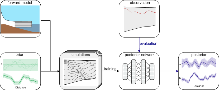
In NPE, we generate a training dataset (Fig. 2) by sampling parameters from the prior and evaluating the forward model . A family of distributions is typically defined in terms of a neural network with learnable weights . We represent as a normalizing flow [Kobyzev \BOthers. (\APACyear2019), Papamakarios \BOthers. (\APACyear2019), Durkan \BOthers. (\APACyear2019)]. The neural network is trained by minimizing the expected negative log-probability
on the training dataset. It has been shown that, under some assumptions, the minimum of this loss is reached when –i.e. when our estimated distribution matches the true posterior [Papamakarios \BBA Murray (\APACyear2016)].
We also make use of an embedding network, which are commonly used in SBI workflows in order to improve performance. Embedding networks learns summary statistics , which are lower-dimensional representations of the data . The embedding network is trained jointly with the normalizing flow. In our setting, are spatially-varying IRH elevations, and so we choose a 1-dimensional convolutional neural network (CNN) as our embedding net, resulting in 50-dimensional embeddings on which the posterior network is conditioned (full details in Appendix C.2).
2.2.2 Details on Model Parameters and Observations
We define , the values of the accumulation rate on a discretized grid . In our experiment, we choose the number of inference grid points as a compromise between computational complexity of the inference problem while still inferring accumulation rate at a high resolution of approximately km. This is smaller than the discretized grid we use for our simulations, which has 500 gridpoints in our experiments. In practice, we take to be a regularly spaced subset of , so that can also be taken as a subset of . However, can be any discretization of the flow line, and need not be a subset of . Furthermore, despite defining to only represent the surface accumulation, any inference of the surface accumulation automatically extends to inference of the basal melt rates. This is because for any probability distribution , the total mass balance relationship implies that , where are the respective discretizations of onto .
We now turn to describing the observation, . The observed data is a set of different IRHs, , where is the elevation of the IRH in our dataset at grid position . The IRH elevations need not and typically are not observed at the same locations as the simulation gridpoints, and so we first interpolate the IRH elevations onto the simulation grid using linear spline interpolation (as implemented in Scipy [Virtanen \BOthers. (\APACyear2020)]). Therefore, w.l.o.g. we assume is already defined on . In our work, we choose to separately infer the mass balance from each IRH in our observed dataset. This has two advantages: first, the number and average depths of picked IRHs in datasets varies between measurements, and cannot be predicted a-priori. Thus, learning some global property about the ice shelf from a set of IRHs is highly challenging. Second, ordering IRHs by depth also corresponds to their reverse age order, with the oldest IRHs being the deepest. Thus, inferring the surface accumulation and basal melt rates for deeper IRHs corresponds to inferring the average rates over longer periods of time. By comparing the inferred mass balance parameters obtained with different IRHs, we can reason about how they changed over time.
Thus, given a dataset of observed IRHs, we have inference problems to solve, where each observation corresponds to one IRH. It is therefore reasonable to take one isochronal layer of the simulated stratigraphy as the output of the forward model. For the inference problem, we define the outcome of forward model as the isochronal layer that is closest to IRH (in the mean square sense). More precisely, for inference problem and simulation , we define the observation of the forward model to be , where
Here, is the index of the boundary of the LMI body for IRH . For the IRH is outside the LMI body and for within the LMI body (see Appendix B.2 for details). We also define as the restriction of the gridpoints to within the LMI body of . We correspondingly set the observation for IRH to .
2.2.3 Choice of Prior Distribution
We aim to approximate the posterior distribution . The likelihood is not analytically tractable, but can be sampled from using the forward model. For Ekström Ice Shelf we use the long-term snow accumulation observations of the Neumayer stations [Wesche \BOthers. (\APACyear2016), Wesche \BBA Regnery (\APACyear2022)] over more than 30 years to define an empirically-motivated prior. We first assume that localized surface melt (), is possible, but rare. We also observe that average rate of accumulation is approximately 0.5 \unitm\unita^-1, and that the accumulation rate is almost everywhere under 2 \unitm\unita^-1. Finally, we take the accumulation rate to vary smoothly in space. As a result of these empirical observations, we define the following generative process as a prior over : first, we draw a sample from a Gaussian process with mean function and a Matérn kernel with a Matérn- of 2.5 and a lengthscale of m [Rasmussen \BBA Williams (\APACyear2005)]. We then independently sample an offset and scale parameter. Finally, we set . We use this prior distribution for both synthetic and Ekström ice shelves.
Defining the prior in this way is sufficiently expressive to capture numerous accumulation rate profiles, while also restricting the samples to conform to empirical knowledge. Additionally, the prior is shared for all inference problems we have defined, and one evaluation of the forward model provides an observation for each of the inference problems. Thus, the same training dataset can be used for all posterior networks in our SBI approach, significantly reducing the computational costs.
2.3 Implementation Details
First, we used Antarctic Mapping Tools [Greene \BOthers. (\APACyear2017)], BedMachine Antarctica [Morlighem \BOthers. (\APACyear2017)], and ITS_LIVE [Gardner \BOthers. (\APACyear2022)] to obtain the surface elevation , thickness and velocity for Ekström Ice Shelf. In order to define the flow tube domain for Ekström Ice Shelf, we also used the itslive_flowline tool to find two flow lines which formed the side-boundaries of the domain. The other two boundaries of the domain were the grounding line, and a straight line connecting the two flow lines. The straight line was chosen to ensure that the radar transect where data was measured is wholly contained within the flow tube domain.
For Ekström ice shelf (Sec. 4) we preprocessed the raw ice shelf geometry and velocity data prior to evaluating the model. This ensured numerical stability of the forward model. Using the icepack package for Python [Shapero \BOthers. (\APACyear2021)], we first smoothed the raw thickness data by solving a regularized minimization problem. We then solved for the best-fitting velocity by fitting a fluidity parameter in an SSA model to the observed velocity and smoothed thickness. In the synthetic example (Section 3), icepack was also used in order to create a steady-state ice shelf. The hyperparameters used for preprocessing are given in Appendix C. Finally, once the training dataset was created, the sbi package for Python [Tejero-Cantero \BOthers. (\APACyear2020)] was used for the inference procedure described in Section 2.2.1.
2.4 Radar Measurements of Internal Stratigraphy
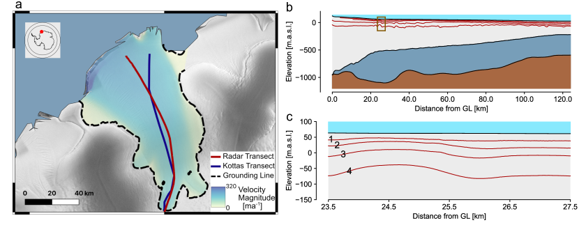
Internal stratigraphy data along the central flow line of Ekström Ice Shelf (Fig. 3a) were acquired using a ground-based ground-penetrating radar with a center frequency of 50 \unitMHz (pulseEKKOTM from Sensors & Software) in two consecutive field seasons (2021/22 and 2022/23) with logistic support from the Neumayer III station [Wesche \BOthers. (\APACyear2016), Wesche \BBA Regnery (\APACyear2022)]. Radar processing was done with ImpDAR [Lilien \BOthers. (\APACyear2020)] and included trace averaging to equidistant spacing (10 \unitm), bandpass filtering (with cut-off frequencies of 20 and 75 \unitMHz), and a topographic correction using the REMA surface elevation [Howat \BOthers. (\APACyear2019)]. The latter provides observations consistent with the modeling setup. The radar detects the ice-ocean interface and continuous internal reflection horizons (IRHs) down to approximately 200 m depth (Fig. 3b and c). Four IRHs were digitized along the entire 130 km long profile using a semi-automatic maximum tracking scheme. The vertical offset off IRHs at the profile junction in the mid-shelf region between both years is much smaller than the radar system’s wavelength in ice ( 3.4 \unitm). Consequently IRHs were connected without adjustments. For the travel-time to depth conversion we used a depth-density profile representative for ice shelves of the Dronning Maud Land Coast (\citeAHubbard2013, Eq. 1).
3 Synthetic Test Case
Before we apply the presented workflow to a real example in Ekström Ice Shelf, we showcase its applicability in a synthetic test case in which the ground truth parameters are known.
3.1 Configuration of Shelf and flow line
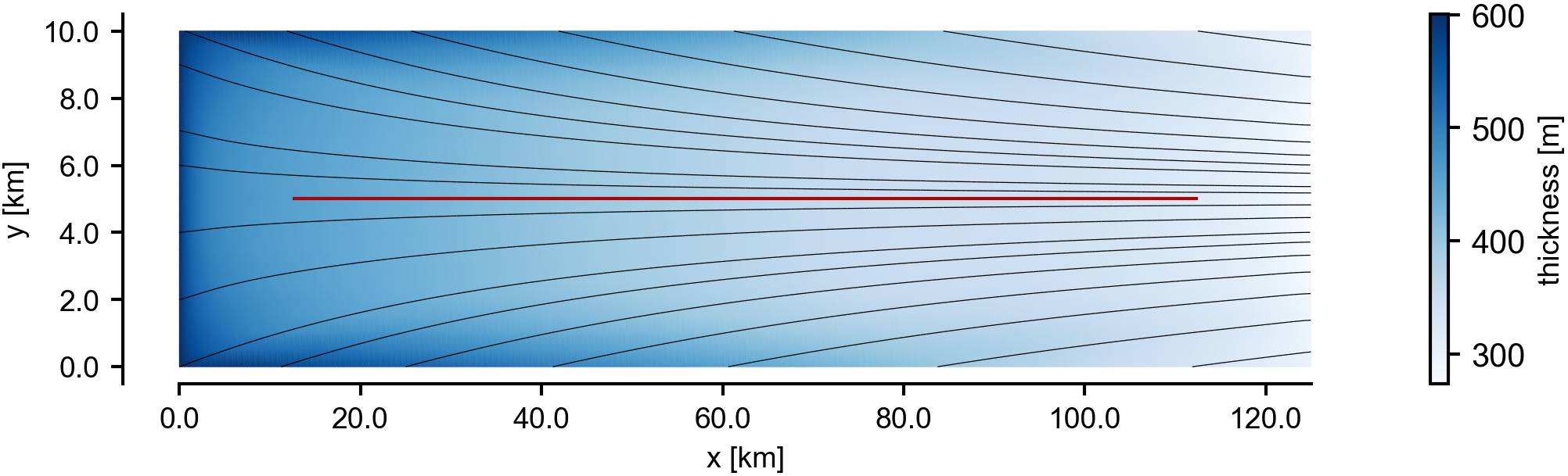
We present a case study on a synthetically-generated flow line. We begin by creating a two dimensional flow tube on a grid \unitkm \unitkm, with the along-flow direction and across-flow direction . We instantiate the flow tube with a Dirichlet boundary condition at the inflow and lateral boundaries, with a constant thickness of , and a constant along-flow velocity of . We mimic lateral boundary conditions with some friction by initializing a zero centered, longitudinally symmetric across-flow velocity on the lateral boundaries, resulting in a flow field that has convergence (i.e. mass input) on the center flow line.
We fix a total mass balance of the shelf, and perform a transient simulation of the resulting flow tube using the SSA approximation, until steady state is reached. From the steady state ice shelf, we choose a discretization of the central flow line, , and extract the relevant variables along this flow line to define the internal stratigraphy model (Fig. 4). The variables we need are the surface and base elevations, the along-flow velocities , and the along- and across-flow flux divergences , . These define the total mass balance, since:
We also use the flux divergences to account for the flow tube correction (Appendix A.1).
We choose an arbitrary sample from the prior distribution as the ground truth, . We calculate the corresponding ground truth basal melt rate profile . The forward model is then sampled to obtain a set of ground truth layer elevations, . From these layer elevations, we choose to perform inference for four layers of ages 50, 100 and 150, and 300 years (labelled 1 to 4 in ascending order of age). These ages roughly correspond to the range of ages of the IRHs that we expect to observe on ice shelves.
3.2 Inference Results
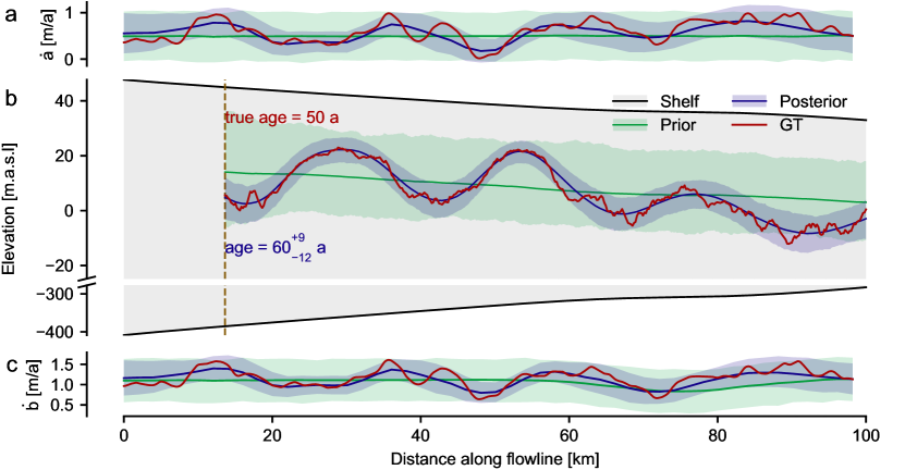
We evaluate the trained neural posterior network on the ground truth isochronal layer of age 50 years. The inferred posterior mean surface accumulation rate is close to the ground truth accumulation rate (Fig. 5a,c) and the ground truth lies within the 95% confidence intervals of the posterior distribution.
Next, we evaluate the forward model on samples from the posterior (and prior) distribution to get the respective predictive distributions. This shows the prior and posterior predictions of the isochronal layer (Fig. 5b). The posterior predictive matches the ground truth isochronal layer with high fidelity. We calculate the root mean square error (RMSE) of the predictive simulations relative to the ground truth layer elevations for 1000 simulations using prior and posterior samples. The average RMSE for the posterior is 3.9 \unitm, compared to 11.5 \unitm for the prior. Uncertainties in the layer elevations are much smaller than those of the prior predictive distribution. This is in contrast to the posterior uncertainty over the mass balance rates, which is still considerable. This showcases the importance of our uncertainty-aware approach: there is more than one parameterization of accumulation and basal melt rates that can lead to similar isochronal layers.
The posterior uncertainty is also reflected in the inferred age of the isochronal layer. We infer an age of years for this layer (meaning a median of 60 years, and 16th and 84th percentiles of 48 and 69 years respectively). This value matches the age of the ground truth isochronal layer, which was not used during inference. Thus we have produced an estimate of the age of the layer without requiring invasive measurements such as ice cores. We report the posterior distributions for deeper synthetic layers in Appendix E.
4 Ekström Ice Shelf
Ekström Ice Shelf is a medium-sized ice shelf located between the Sörasen and Halvfarryggen Ice Rises in Dronning Maud Land, East Antarctica (Fig. 3 C). Ekström Ice Shelf makes for an appropriate study site because the steady-state assumption likely holds [Drews \BOthers. (\APACyear2013)], and because it is well modelled by the shallow shelf approximation [Schannwell \BOthers. (\APACyear2019)]. Moreover, because of the proximity of the Neumayer station III numerous observations are available, e.g. ice thickness, surface velocities and most importantly surface accumulation rates, which we will use later for validation.
4.1 Inference Results
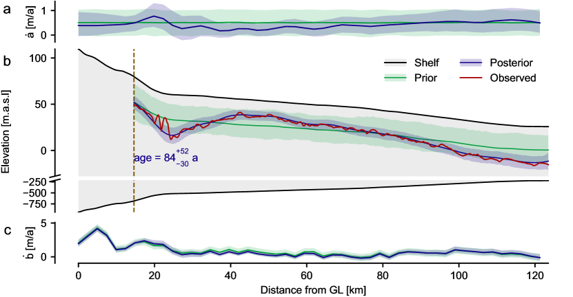
We inspect the prior over the basal melt rates as a validation of our modeling choices. The implicit prior is the same as the prior defined for the surface accumulation, with the mean shifted by the total mass balance on the flow line, . The basal melt rate is larger (up to 4 \unitm\unita^-1) near the grounding line, and gradually stabilises in the along-flow direction to values between 0 and 1 \unitm\unita^-1 downstream. This is in agreement with previous estimates for basal melt profiles on this particular ice shelf [Neckel \BOthers. (\APACyear2012)].
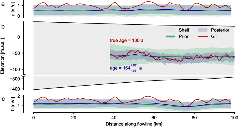
We infer the surface accumulation and basal melt rates from IRH 2 in our dataset, which has an average (ice equivalent) depth of 30 \unitm (Fig. 6). The posterior over the surface accumulation rate has uncertainty comparable to that of the prior. However, there is a shift in the overall spatial trend of the accumulation rate; particularly, there is higher surface accumulation rate at approximately 20 \unitkm from the grounding line. Accumulation rate also increases steadily downstream the flow line. As in the synthetic case, the posterior predictive distribution reproduces the observed IRH with much higher fidelity and confidence than the prior predictive distribution. The average RMSE relative to the observed IRH is 4.6 \unitm for 1000 posterior predictive simulations, compared to 11.8 \unitm for 1000 prior predictive simulations. The posterior predictive produces an independent estimate of the unknown age of the IRH of years.
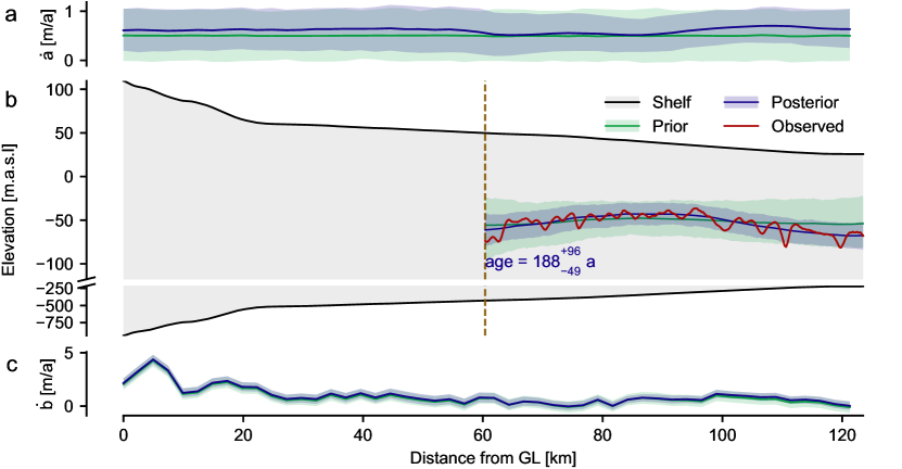
Our method can use much deeper IRHs for the inference of accumulation and basal melt rates. For IRH 4 of the observed dataset (of average depth 131 m), the proportion of the IRH that is within the LMI body is smaller. This is due to the unknown boundary condition influencing the IRH elevation at much further points along the flow line. This discarding of data has visible effects on our parameter posterior (Fig. 7), which now is more similar to the prior near the grounding line, and only diverges at points further down the ice shelf, where the values of accumulation and basal melt rates affect the dynamics of the IRH. Regardless, the posterior predictive reconstructs the observed IRH at higher fidelity and precision than the prior predictive. The average RMSE relative to the observed IRH is 10.0 \unitm for the posterior and 16.4 \unitm for the prior. The estimated age of this IRH by our method is years. The uncertainty of the age estimates reasonably increases for deeper IRHs.
5 Discussion
5.1 Ekström Ice Shelf is in Steady State
We compare the four posteriors over the surface accumulation obtained from the Ekström IRH dataset (Fig. 8). The posteriors for the shallower IRHs 1–3 all show a similar qualitative relationship: a local maximum of the accumulation at a distance of approximately 20 \unitkm from the grounding line, followed by a steady increase in the accumulation downstream. This supports our initial assumption that Ekström Ice Shelf is in steady state. Additionally, the increase in accumulation at 20 \unitkm is even identified in the posterior for IRH 3, despite the LMI boundary being downstream of it, at approximately 30 \unitkm from the grounding line. This is reasonable, as the mass balance parameters at a given location affect the flow field downstream of this location, and consequently, the formation of isochronal layers. For IRH 4, the LMI boundary is much further downstream at 60 \unitkm. Thus, the local surface accumulation maximum at 20 \unitkm is not found, however the overall trend of increasing surface accumulation downstream is still identified. The corresponding trend in the basal melt rate is dominated by the total mass balance, . However, the basal melt rate still exhibits a local maximum at 20 \unitkm. This could be related to increased tidal forces in the flexure zone of the ice shelf.
The inferred posteriors also allow us to estimate the age of the IRHs. By sampling from the posterior distribution, and evaluating the forward model with the resulting mass balance parameter samples, we obtain a distribution of isochronal layers similar to the observed IRH, with known ages. Thus, we estimate the ages of the four IRHs as 42, 84, 146 and 188 years. Our results therefore support the assumption that Ekström Ice Shelf has been in steady state for the past 188 years. Crucially, we are able to estimate the age of the IRHs without invasive measurements such as ice cores. This estimate depends on a realistic prior for the surface and basal mass balance, as defined in Sec. 2.2.3. Given a miscalibrated prior, the estimated ages would not be reliable (see Appendix G for an example). We hypothesise that given an independent measurement of the age of the IRH, our approach could constrain the posterior distributions over the mass balance parameters further.
5.2 Comparison to Shallow and Local Layer Approximations, and Kottas Traverse Accumulation Measurements
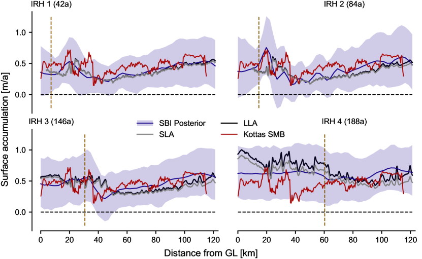
To validate our approach, we compare the inferred surface accumulation rate of our experiments with estimates from other methods. First, we computed the Shallow Layer Approximation (SLA) and Local Layer Approximation (LLA) as described in \citeAWaddington2007. Given the depth and age of IRH , the SLA and LLA approximations for the accumulation rate are defined as
where is the age of IRH . Intuitively, the SLA takes the ice thickness above layer and divides it by the layer age, whereas LLA accounts for strain thinning assuming a linear vertical velocity profile (which is often the case for ice-shelf flow). Since the age of the observed IRHs is not known, we use the median age of the posterior predictive distribution results. As expected, we observe that both SLA and LLA closely match the SBI posterior mean accumulation rate for the shallow IRHs of estimated ages 42, 84 years (Fig. 8). As the strain rates of the flow are small, the relatively shallow IRHs (mean ice equivalent depth of 30 \unitm) have not notably deformed, and hence the assumptions of SLA and LLA are appropriate. However, for the deeper IRHs 3 and 4 of estimated ages 146 and 188 years, we see that both SLA and LLA estimates diverge from our posterior mean accumulation rate. This shows that more involved approaches are required when using deeper IRHs for inference. For deeper IRHs where the SLA and LLA no longer applied, \citeASteen-Larsen2010 inferred the surface accumulation rates on grounded ice using a Monte Carlo approach. By treating the age of the IRH as an additional parameter to infer, they were able to identify the age of the IRH with high confidence. Extensions of our approach could incorporate this parameterization to reduce the uncertainty of the inferred IRH.
For the Ekström transect comparison data is provided by repeat readings of accumulation stakes in 500 \unitm spacing along the nearby Kottas traverse (Fig. 8). Yearly readings are available in the period 1996–2005 and on a yearly to three-yearly interval between 2014–2023 [Mengert (\APACyear2018)]. We use this dataset to construct a direct estimate of time-averaged surface accumulation rate along the central flow line transect. For this, we project the measurements from the Kottas traverse to the flow line transect, taking into account an increased uncertainty for increasing projection distance (see Appendix F for details).
The Kottas traverse accumulation measurements closely match the posterior means of our approach (Fig. 8) for IRHs 1 and 2. As the accumulation rate measurements on the Kottas traverse span the past 26 years it may not be a good validation for the deeper IRHs. Regardless, the Kottas accumulation rate measurements lie within the posterior uncertainty for IRHs 3 and 4. These comparisons further corroborate our approach and highlight the advantages of uncertainty-aware methods, especially as the measured accumulation rates also varied considerably year-to-year (Appendix F).
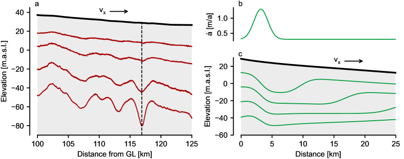
5.3 Future Directions for Forward Modeling Approach
The fidelity at which the posterior predictive distributions reproduce the observed IRHs of Ekström Ice Shelf (Figs. 6, 7) justify our modeling choices for this ice shelf, as the combination of the forward model and accumulation rate prior distribution are sufficiently expressive to reproduce the IRHs. However, we see that local perturbations in the IRH elevations are amplified for deeper IRHs in the observed dataset (Fig. 9c). This is in contrast to the layer tracing model (Fig. 9b), where the layer elevation perturbations are transported by the flow without amplification. Thus, a Lagrangian scheme, which takes the flow velocity into account, could be beneficial to parameterize accumulation rates and capture this behaviour in future work. In such a scheme, the surface accumulation profile would be coupled to the ice shelf surface topography. This approach is supported by studies of the atmospheric forcing that determines surface accumulation [Gow \BBA Rowland (\APACyear1965), Dattler \BOthers. (\APACyear2019)], which suggest that local features in the surface topography can cause local surface accumulation perturbations. In the plug flow regime of the shelf, the isochronal layers are transported at the same speed as the surface. Hence a local perturbation in the surface accumulation would continue to amplify local perturbations in the isochronal layer elevations. This would be captured by a Lagrangian parameterization scheme.
Although the steady state assumption was appropriate for Ekström Ice Shelf, it will need to be relaxed in order to apply our methodology to non-steady state flow regimes. While it is possible to couple the layer tracing scheme to an external solver of ice dynamics (e.g., \citeABorn2021), the main challenge will be the added computational cost of modeling ice flow as opposed to only the steady state internal stratigraphy. Here, a new family of fast ice flow solvers could be of great use [Sandip \BOthers. (\APACyear2023)]. An alternative approach is probabilistic numerics, in which the forward and inverse problems are solved simultaneously [Krämer \BOthers. (\APACyear2022), Hennig \BOthers. (\APACyear2022)]. Finally, the forward model can be extended to remove the plug flow assumption, to allow for depth-dependent velocities. This would allow our approach to be applied to grounded ice.
5.4 Simulation Based Inference as a Tool for Geoscientific Inversion Problems
The inverse problem tackled in this work typifies geoscientific inverse problems, as the forward model is defined in terms of a partial differential equation (PDE), and the parameters are high dimensional and vary in space. Hence, it is valuable to compare the SBI approach in this case to the wide variety of methods and algorithms that have been developed to solve geoscientific inverse problems.
The SBI approach as presented here has two key features. First, we estimate the Bayesian posterior distribution, providing quantitative uncertainty estimates. Modeling uncertainty is important as it can highly influence and propagate to future modeling predictions. Additionally, locations of high uncertainty show areas requiring further study, helping to guide future work. In contrast, deterministic inference methods typically only attempt to infer a single estimate of best-fitting parameters, e.g., the maximum likelihood estimate (MLE), and provide no measure of uncertainty. Estimates of uncertainty are also present in other inference approaches, for example in Markov Chain Monte Carlo (MCMC, \citeAGallagher2009), Bayesian filtering approaches [Stordal \BOthers. (\APACyear2011), van Leeuwen \BOthers. (\APACyear2019)], and variational inference [Zhang \BOthers. (\APACyear2021)]. However, these methods require knowledge of the likelihood function of the forward model. For computationally complex forward models, such as PDE solvers, the likelihood is often computationally intractable. The SBI approach performs approximate Bayesian computation (ABC, \citeARubin1984,Sisson2018), and only requires us to be able to evaluate the forward model. Thus, ABC methods can be applied to a larger class of inference problems. Second, a unique advantage of single round SBI methods [Cranmer \BOthers. (\APACyear2020)] such as NPE (as used in our study) is amortization. An amortized inference framework is one that, once trained, can be applied to find the posterior distribution for any measurement without any additional simulation or training costs. Our method as presented here is not yet fully amortized as preprocessing relies on the observed value of : in order to train the density estimator , we first calculate for each simulation dependent on the value of . Regardless, our method still amortizes the cost of simulating the forward model many times, which is by far the largest computational cost in the approach. In particular, we solved parallel inference problems that shared the same prior distribution, and where the forward model could output the observations in one evaluation. Therefore, the same set of simulations was shared for all inference problems. In the Ekström example, we have evaluated the forward model a total of 190,000 times, accounting for approximately 99% of the total computation cost (D). Thus, we have amortized the majority of the computational cost of inference.
On the other hand, SBI faces some limitations as an inference tool. Primarily, SBI methods are known to require a large number of simulations to be trained, [Lueckmann \BOthers. (\APACyear2021)]. Performing on the order of simulations would not have been feasible for forward models of higher computational complexity. Moreover, SBI methods scale poorly in number of simulations required as the size of the parameter vector increases. The SBI approach needs to be adapted to more efficiently represent high-dimensional, spatially varying parameters at high resolutions. Some potential approaches are polynomial or spectral representations. Future work should also explore variants of SBI that are better suited to high-dimensional or even continuous parameters [Ramesh \BOthers. (\APACyear2022), Geffner \BOthers. (\APACyear2022)]. Finally, SBI works under the assumption that the forward model is well-specified, meaning that given samples from the prior, it can generate simulations closely resembling the observation. The posteriors obtained by SBI can be strongly biased when this is not the case [Cannon \BOthers. (\APACyear2022)]. Work to address this concern has been done, e.g. by incorporating the model mismatch into the forward model [Ward \BOthers. (\APACyear2022)], as done in our work using the calibrated noise model.
6 Conclusions
We presented a novel approach for inferring the spatially-varying surface accumulation and basal melt rates along ice shelf flow lines from radar measurements of their internal stratigraphy. We validated the method on a synthetic ice shelf example, and inferred the surface accumulation and basal melt rates along a flow line in Ekström Ice Shelf, Antarctica. We separately inferred the mass balance parameters from four different internal reflection horizons, obtaining posterior distributions consistent with a steady state ice shelf. The inferred distributions were further validated by independent stake array measurements of surface accumulation rates uniquely available in Ekström Ice Shelf. Using our approach, we were able to estimate the otherwise unknown age of the internal reflection horizons as 42, 84, 146 and 188 years. The presented approach can be transferred to other Antarctic ice shelves, and also to other flow regimes such as grounded ice. A strength of our approach is the principled uncertainty estimates in the inferred surface accumulation and basal melt rates. Uncertainty estimates can be integrated in future projections of the Antarctic Ice Sheet [Verjans \BOthers. (\APACyear2022), Ultee \BOthers. (\APACyear2023)]. We identified avenues for future work as more can be learned by relaxing the steady state assumption on the ice shelf. The forward model and inference framework should be adapted to account for potential transient signals in the mass balance parameters.
This work was an example use case of SBI for a geoscientific inverse problem. We showcased the strengths of SBI as a likelihood-free approach to approximate the Bayesian posterior, amortizing the cost of simulating the forward model many times. SBI can become more applicable to such inverse problems involving spatially- (and temporally-) varying parameters if it can be extended to deal with the challenge of high-dimensional parameter inference.
Finally, our approach highlights the value of internal stratigraphy measurements. Initiatives to map the Antarctic-wide internal stratigraphy (e.g. \citeAAntArchitecture) can provide invaluable data towards uncovering the history of the Antarctic ice sheet. Sophisticated inference methods could be combined with such a dataset to provide a new, independent, Antarctica-wide parameterization of accumulation and basal melt rate histories.
Open Research
Data Availability Statement
Simulation data available at https://doi.org/doi:10.5281/zenodo.10245153.
Software Availability
Code for preprocessing Ekström ice shelf data and generating synthetic ice shelf data available at https://github.com/mackelab/preprocessing-ice-data.
Code for layer tracing forward model and simulation-based inference workflow available at https://github.com/mackelab/sbi-ice.
Acknowledgements.
The authors would like to thank Daniel Shapero for his inputs on use of icepack. The authors would also like to thank Andreas Born and Therese Riekch for insightful discussions on the implementation of the layer tracing solver for calculating internal stratigraphy. We acknowledge excellent logistic support from staff at Neumayer III station and the GrouZe team on-site. This work was funded by the German Research Foundation (DFG) under Germany’s Excellence Strategy – EXC number 2064/1 – 390727645 and SFB 1233 ’Robust Vision’ (276693517) and the German Federal Ministry of Education and Research (BMBF): Tübingen AI Center, FKZ: 01IS18039A. Reinhard Drews and Vjeran Višnjević were supported by an Emmy Noether grant of the Deutsche Forschungsgemeinschaft (DR 822/3-1). We acknowledge the support by the German Academic Scholarship Foundation to Falk M. Oraschewski. Guy Moss is a member of the International Max Planck Research School for Intelligent Systems (IMPRS-IS).References
- Adusumilli \BOthers. (\APACyear2020) \APACinsertmetastarAdusumilli2020{APACrefauthors}Adusumilli, S., Fricker, H\BPBIA., Medley, B., Padman, L.\BCBL \BBA Siegfried, M\BPBIR. \APACrefYearMonthDay20208. \BBOQ\APACrefatitleInterannual variations in meltwater input to the Southern Ocean from Antarctic ice shelves Interannual variations in meltwater input to the southern ocean from antarctic ice shelves.\BBCQ \APACjournalVolNumPagesNature Geoscience 2020 13:913616-620. {APACrefDOI} 10.1038/s41561-020-0616-z \PrintBackRefs\CurrentBib
- Agosta \BOthers. (\APACyear2019) \APACinsertmetastarAgosta2019{APACrefauthors}Agosta, C., Amory, C., Kittel, C., Orsi, A., Favier, V., Gallée, H.\BDBLFettweis, X. \APACrefYearMonthDay2019. \BBOQ\APACrefatitleEstimation of the Antarctic surface mass balance using the regional climate model MAR (1979–2015) and identification of dominant processes Estimation of the antarctic surface mass balance using the regional climate model mar (1979–2015) and identification of dominant processes.\BBCQ \APACjournalVolNumPagesThe Cryosphere131281–296. {APACrefDOI} 10.5194/tc-13-281-2019 \PrintBackRefs\CurrentBib
- Allgeier \BBA Cirpka (\APACyear2023) \APACinsertmetastarAllgeier2023{APACrefauthors}Allgeier, J.\BCBT \BBA Cirpka, O\BPBIA. \APACrefYearMonthDay2023. \BBOQ\APACrefatitleSurrogate-Model Assisted Plausibility-Check, Calibration, and Posterior-Distribution Evaluation of Subsurface-Flow Models Surrogate-model assisted plausibility-check, calibration, and posterior-distribution evaluation of subsurface-flow models.\BBCQ \APACjournalVolNumPagesWater Resources Research597. {APACrefDOI} https://doi.org/10.1029/2023WR034453 \PrintBackRefs\CurrentBib
- Asay-Davis \BOthers. (\APACyear2016) \APACinsertmetastarAsay-Davis2016{APACrefauthors}Asay-Davis, X\BPBIS., Cornford, S\BPBIL., Durand, G., Galton-Fenzi, B\BPBIK., Gladstone, R\BPBIM., Gudmundsson, G\BPBIH.\BDBLSeroussi, H. \APACrefYearMonthDay20167. \BBOQ\APACrefatitleExperimental design for three interrelated marine ice sheet and ocean model intercomparison projects: MISMIP v. 3 (MISMIP +), ISOMIP v. 2 (ISOMIP +) and MISOMIP v. 1 (MISOMIP1) Experimental design for three interrelated marine ice sheet and ocean model intercomparison projects: Mismip v. 3 (mismip +), isomip v. 2 (isomip +) and misomip v. 1 (misomip1).\BBCQ \APACjournalVolNumPagesGeoscientific Model Development92471-2497. {APACrefDOI} 10.5194/GMD-9-2471-2016 \PrintBackRefs\CurrentBib
- Berger \BOthers. (\APACyear2017) \APACinsertmetastarBerger2017{APACrefauthors}Berger, S., Drews, R., Helm, V., Sun, S.\BCBL \BBA Pattyn, F. \APACrefYearMonthDay201711. \BBOQ\APACrefatitleDetecting high spatial variability of ice shelf basal mass balance, Roi Baudouin Ice Shelf, Antarctica Detecting high spatial variability of ice shelf basal mass balance, roi baudouin ice shelf, antarctica.\BBCQ \APACjournalVolNumPagesCryosphere112675-2690. {APACrefDOI} 10.5194/tc-11-2675-2017 \PrintBackRefs\CurrentBib
- Bindschadler \BOthers. (\APACyear2011) \APACinsertmetastarBindschadler2011{APACrefauthors}Bindschadler, R., Choi, H., Wichlacz, A., Bingham, R., Bohlander, J., Brunt, K.\BDBLYoung, N. \APACrefYearMonthDay2011. \BBOQ\APACrefatitleGetting around Antarctica: New high-resolution mappings of the grounded and freely-floating boundaries of the Antarctic ice sheet created for the International Polar Year Getting around antarctica: New high-resolution mappings of the grounded and freely-floating boundaries of the antarctic ice sheet created for the international polar year.\BBCQ \APACjournalVolNumPagesCryosphere5569-588. {APACrefDOI} 10.5194/TC-5-569-2011 \PrintBackRefs\CurrentBib
- Bingham \BOthers. (\APACyear2019) \APACinsertmetastarAntArchitecture{APACrefauthors}Bingham, R\BPBIG., Eisen, O., Karlsson, N\BPBIB., MacGregor, J\BPBIA., Ross, N.\BCBL \BBA Young, D\BPBIA. \APACrefYearMonthDay2019July. \BBOQ\APACrefatitleAntArchitecture: an international project to use Antarctic englacial layering to interrogate stability of the Antarctic Ice Sheets Antarchitecture: an international project to use antarctic englacial layering to interrogate stability of the antarctic ice sheets.\BBCQ \BIn \APACrefbtitleIGS Symposium Five Decades of Radioglaciology. Igs symposium five decades of radioglaciology. \PrintBackRefs\CurrentBib
- Born (\APACyear2017) \APACinsertmetastarBorn2017{APACrefauthors}Born, A. \APACrefYearMonthDay20172. \BBOQ\APACrefatitleTracer transport in an isochronal ice-sheet model Tracer transport in an isochronal ice-sheet model.\BBCQ \APACjournalVolNumPagesJournal of Glaciology6322-38. {APACrefDOI} 10.1017/JOG.2016.111 \PrintBackRefs\CurrentBib
- Born \BBA Robinson (\APACyear2021) \APACinsertmetastarBorn2021{APACrefauthors}Born, A.\BCBT \BBA Robinson, A. \APACrefYearMonthDay20219. \BBOQ\APACrefatitleModeling the Greenland englacial stratigraphy Modeling the greenland englacial stratigraphy.\BBCQ \APACjournalVolNumPagesCryosphere154539-4556. {APACrefDOI} 10.5194/TC-15-4539-2021 \PrintBackRefs\CurrentBib
- Burgard \BOthers. (\APACyear2022) \APACinsertmetastarBurgard2022{APACrefauthors}Burgard, C., Jourdain, N\BPBIC., Reese, R., Jenkins, A.\BCBL \BBA Mathiot, P. \APACrefYearMonthDay202212. \BBOQ\APACrefatitleAn assessment of basal melt parameterisations for Antarctic ice shelves An assessment of basal melt parameterisations for antarctic ice shelves.\BBCQ \APACjournalVolNumPagesCryosphere164931-4975. {APACrefDOI} 10.5194/TC-16-4931-2022 \PrintBackRefs\CurrentBib
- Cannon \BOthers. (\APACyear2022) \APACinsertmetastarCannon2022{APACrefauthors}Cannon, P., Ward, D.\BCBL \BBA Schmon, S\BPBIM. \APACrefYearMonthDay2022\APACmonth09. \BBOQ\APACrefatitleInvestigating the Impact of Model Misspecification in Neural Simulation-based Inference Investigating the Impact of Model Misspecification in Neural Simulation-based Inference.\BBCQ \APACjournalVolNumPagesarXiv e-printsarXiv:2209.01845. {APACrefDOI} 10.48550/arXiv.2209.01845 \PrintBackRefs\CurrentBib
- Catania \BOthers. (\APACyear2010) \APACinsertmetastarCatania2010{APACrefauthors}Catania, G., Hulbe, C.\BCBL \BBA Conway, H. \APACrefYearMonthDay2010. \BBOQ\APACrefatitleGrounding-line basal melt rates determined using radar-derived internal stratigraphy Grounding-line basal melt rates determined using radar-derived internal stratigraphy.\BBCQ \APACjournalVolNumPagesJournal of Glaciology56197545–554. {APACrefDOI} 10.3189/002214310792447842 \PrintBackRefs\CurrentBib
- Cranmer \BOthers. (\APACyear2020) \APACinsertmetastarCranmer2020{APACrefauthors}Cranmer, K., Brehmer, J.\BCBL \BBA Louppe, G. \APACrefYearMonthDay2020. \BBOQ\APACrefatitleThe frontier of simulation-based inference The frontier of simulation-based inference.\BBCQ \APACjournalVolNumPagesProceedings of the National Academy of Sciences1174830055-30062. {APACrefDOI} 10.1073/pnas.1912789117 \PrintBackRefs\CurrentBib
- Das \BOthers. (\APACyear2020) \APACinsertmetastarDas2020{APACrefauthors}Das, I., Padman, L., Bell, R\BPBIE., Fricker, H\BPBIA., Tinto, K\BPBIJ., Hulbe, C\BPBIL.\BDBLSiegfried, M\BPBIR. \APACrefYearMonthDay2020. \BBOQ\APACrefatitleMultidecadal Basal Melt Rates and Structure of the Ross Ice Shelf, Antarctica, Using Airborne Ice Penetrating Radar Multidecadal basal melt rates and structure of the ross ice shelf, antarctica, using airborne ice penetrating radar.\BBCQ \APACjournalVolNumPagesJournal of Geophysical Research: Earth Surface1253e2019JF005241. {APACrefDOI} https://doi.org/10.1029/2019JF005241 \PrintBackRefs\CurrentBib
- Dattler \BOthers. (\APACyear2019) \APACinsertmetastarDattler2019{APACrefauthors}Dattler, M\BPBIE., Lenaerts, J\BPBIT\BPBIM.\BCBL \BBA Medley, B. \APACrefYearMonthDay2019. \BBOQ\APACrefatitleSignificant Spatial Variability in Radar-Derived West Antarctic Accumulation Linked to Surface Winds and Topography Significant spatial variability in radar-derived west antarctic accumulation linked to surface winds and topography.\BBCQ \APACjournalVolNumPagesGeophysical Research Letters462213126-13134. {APACrefDOI} https://doi.org/10.1029/2019GL085363 \PrintBackRefs\CurrentBib
- Depoorter \BOthers. (\APACyear2013) \APACinsertmetastarDepoorter2013{APACrefauthors}Depoorter, M\BPBIA., Bamber, J\BPBIL., Griggs, J\BPBIA., Lenaerts, J\BPBIT\BPBIM., Ligtenberg, S\BPBIR., Broeke, M\BPBIR\BPBIV\BPBID.\BCBL \BBA Moholdt, G. \APACrefYearMonthDay20139. \BBOQ\APACrefatitleCalving fluxes and basal melt rates of Antarctic ice shelves Calving fluxes and basal melt rates of antarctic ice shelves.\BBCQ \APACjournalVolNumPagesNature 2013 502:746950289-92. {APACrefDOI} 10.1038/nature12567 \PrintBackRefs\CurrentBib
- Drews (\APACyear2015) \APACinsertmetastarDrews2015channels{APACrefauthors}Drews, R. \APACrefYearMonthDay20156. \BBOQ\APACrefatitleEvolution of ice-shelf channels in Antarctic ice shelves Evolution of ice-shelf channels in antarctic ice shelves.\BBCQ \APACjournalVolNumPagesCryosphere91169-1181. {APACrefDOI} 10.5194/TC-9-1169-2015 \PrintBackRefs\CurrentBib
- Drews \BOthers. (\APACyear2016) \APACinsertmetastarDrews2016{APACrefauthors}Drews, R., Brown, J., Matsuoka, K., Witrant, E., Philippe, M., Hubbard, B.\BCBL \BBA Pattyn, F. \APACrefYearMonthDay2016. \BBOQ\APACrefatitleConstraining variable density of ice shelves using wide-angle radar measurements Constraining variable density of ice shelves using wide-angle radar measurements.\BBCQ \APACjournalVolNumPagesThe Cryosphere102811–823. {APACrefDOI} 10.5194/tc-10-811-2016 \PrintBackRefs\CurrentBib
- Drews \BOthers. (\APACyear2013) \APACinsertmetastarDrews2013{APACrefauthors}Drews, R., Martín, C., Steinhage, D.\BCBL \BBA Eisen, O. \APACrefYearMonthDay2013. \BBOQ\APACrefatitleCharacterizing the glaciological conditions at Halvfarryggen ice dome, Dronning Maud Land, Antarctica Characterizing the glaciological conditions at halvfarryggen ice dome, dronning maud land, antarctica.\BBCQ \APACjournalVolNumPagesJournal of Glaciology592139–20. {APACrefDOI} 10.3189/2013JoG12J134 \PrintBackRefs\CurrentBib
- Drews \BOthers. (\APACyear2015) \APACinsertmetastarDrews2015evolution{APACrefauthors}Drews, R., Matsuoka, K., Martín, C., Callens, D., Bergeot, N.\BCBL \BBA Pattyn, F. \APACrefYearMonthDay20153. \BBOQ\APACrefatitleEvolution of Derwael Ice Rise in Dronning Maud Land, Antarctica, over the last millennia Evolution of derwael ice rise in dronning maud land, antarctica, over the last millennia.\BBCQ \APACjournalVolNumPagesJournal of Geophysical Research: Earth Surface120564-579. {APACrefDOI} 10.1002/2014JF003246 \PrintBackRefs\CurrentBib
- Durkan \BOthers. (\APACyear2019) \APACinsertmetastarDurkan2019{APACrefauthors}Durkan, C., Bekasov, A., Murray, I.\BCBL \BBA Papamakarios, G. \APACrefYearMonthDay2019\APACmonth06. \BBOQ\APACrefatitleNeural Spline Flows Neural Spline Flows.\BBCQ \APACjournalVolNumPagesarXiv e-printsarXiv:1906.04032. {APACrefDOI} 10.48550/arXiv.1906.04032 \PrintBackRefs\CurrentBib
- Dutrieux \BOthers. (\APACyear2014) \APACinsertmetastarDutrieux2014{APACrefauthors}Dutrieux, P., Stewart, C., Jenkins, A., Nicholls, K\BPBIW., Corr, H\BPBIF., Rignot, E.\BCBL \BBA Steffen, K. \APACrefYearMonthDay20148. \BBOQ\APACrefatitleBasal terraces on melting ice shelves Basal terraces on melting ice shelves.\BBCQ \APACjournalVolNumPagesGeophysical Research Letters415506-5513. {APACrefDOI} 10.1002/2014GL060618 \PrintBackRefs\CurrentBib
- Eisen (\APACyear2008) \APACinsertmetastarEisen2008Inference{APACrefauthors}Eisen, O. \APACrefYearMonthDay2008. \BBOQ\APACrefatitleInference of velocity pattern from isochronous layers in firn, using an inverse method Inference of velocity pattern from isochronous layers in firn, using an inverse method.\BBCQ \APACjournalVolNumPagesJournal of Glaciology54187613–630. {APACrefDOI} 10.3189/002214308786570818 \PrintBackRefs\CurrentBib
- Eisen \BOthers. (\APACyear2008) \APACinsertmetastarEisen2008Review{APACrefauthors}Eisen, O., Frezzotti, M., Genthon, C., Isaksson, E., Magand, O., van den Broeke, M\BPBIR.\BDBLVaughan, D\BPBIG. \APACrefYearMonthDay2008. \BBOQ\APACrefatitleGround-based measurements of spatial and temporal variability of snow accumulation in East Antarctica Ground-based measurements of spatial and temporal variability of snow accumulation in east antarctica.\BBCQ \APACjournalVolNumPagesReviews of Geophysics462. {APACrefDOI} https://doi.org/10.1029/2006RG000218 \PrintBackRefs\CurrentBib
- Eisen \BOthers. (\APACyear2004) \APACinsertmetastarEisen2004{APACrefauthors}Eisen, O., Nixdorf, U., Wilhelms, F.\BCBL \BBA Miller, H. \APACrefYearMonthDay20044. \BBOQ\APACrefatitleAge estimates of isochronous reflection horizons by combining ice core, survey, and synthetic radar data Age estimates of isochronous reflection horizons by combining ice core, survey, and synthetic radar data.\BBCQ \APACjournalVolNumPagesJournal of Geophysical Research: Solid Earth1094106. {APACrefDOI} 10.1029/2003JB002858 \PrintBackRefs\CurrentBib
- Gallagher \BOthers. (\APACyear2009) \APACinsertmetastarGallagher2009{APACrefauthors}Gallagher, K., Charvin, K., Nielsen, S., Sambridge, M.\BCBL \BBA Stephenson, J. \APACrefYearMonthDay2009. \BBOQ\APACrefatitleMarkov chain Monte Carlo (MCMC) sampling methods to determine optimal models, model resolution and model choice for Earth Science problems Markov chain monte carlo (mcmc) sampling methods to determine optimal models, model resolution and model choice for earth science problems.\BBCQ \APACjournalVolNumPagesMarine and Petroleum Geology264525-535. {APACrefDOI} https://doi.org/10.1016/j.marpetgeo.2009.01.003 \PrintBackRefs\CurrentBib
- Gallée \BBA Schayes (\APACyear1994) \APACinsertmetastarGallee1994{APACrefauthors}Gallée, H.\BCBT \BBA Schayes, G. \APACrefYearMonthDay1994. \BBOQ\APACrefatitleDevelopment of a Three-Dimensional Meso- Primitive Equation Model: Katabatic Winds Simulation in the Area of Terra Nova Bay, Antarctica Development of a three-dimensional meso- primitive equation model: Katabatic winds simulation in the area of terra nova bay, antarctica.\BBCQ \APACjournalVolNumPagesMonthly Weather Review1224671 - 685. {APACrefDOI} https://doi.org/10.1175/1520-0493(1994)122¡0671:DOATDM¿2.0.CO;2 \PrintBackRefs\CurrentBib
- Gardner \BOthers. (\APACyear2022) \APACinsertmetastarITS_LIVE{APACrefauthors}Gardner, A., Fahnestock, M.\BCBL \BBA Scambos., T. \APACrefYearMonthDay2022. \APACrefbtitleMEaSUREs ITS_LIVE Landsat Image-Pair Glacier and Ice Sheet Surface Velocities, Version 1. Measures its_live landsat image-pair glacier and ice sheet surface velocities, version 1. \APACaddressPublisherNASA National Snow and Ice Data Center Distributed Active Archive Center. {APACrefDOI} 10.5067/IMR9D3PEI28U \PrintBackRefs\CurrentBib
- Geffner \BOthers. (\APACyear2022) \APACinsertmetastarGeffner2022{APACrefauthors}Geffner, T., Papamakarios, G.\BCBL \BBA Mnih, A. \APACrefYearMonthDay2022\APACmonth09. \BBOQ\APACrefatitleCompositional Score Modeling for Simulation-based Inference Compositional Score Modeling for Simulation-based Inference.\BBCQ \APACjournalVolNumPagesarXiv e-printsarXiv:2209.14249. {APACrefDOI} 10.48550/arXiv.2209.14249 \PrintBackRefs\CurrentBib
- Gladstone \BOthers. (\APACyear2021) \APACinsertmetastarGladstone2021{APACrefauthors}Gladstone, R., Galton-Fenzi, B., Gwyther, D., Zhou, Q., Hattermann, T., Zhao, C.\BDBLMoore, J. \APACrefYearMonthDay20212. \BBOQ\APACrefatitleThe Framework for Ice Sheet-Ocean Coupling (FISOC) V1.1 The framework for ice sheet-ocean coupling (fisoc) v1.1.\BBCQ \APACjournalVolNumPagesGeoscientific Model Development14889-905. {APACrefDOI} 10.5194/GMD-14-889-2021 \PrintBackRefs\CurrentBib
- Goelzer \BOthers. (\APACyear2016) \APACinsertmetastarGoezler2016{APACrefauthors}Goelzer, H., Huybrechts, P., Loutre, M\BHBIF.\BCBL \BBA Fichefet, T. \APACrefYearMonthDay2016. \BBOQ\APACrefatitleLast Interglacial climate and sea-level evolution from a coupled ice sheet–climate model Last interglacial climate and sea-level evolution from a coupled ice sheet–climate model.\BBCQ \APACjournalVolNumPagesClimate of the Past12122195–2213. {APACrefDOI} 10.5194/cp-12-2195-2016 \PrintBackRefs\CurrentBib
- Goldberg \BOthers. (\APACyear2019) \APACinsertmetastarGoldberg2019{APACrefauthors}Goldberg, D\BPBIN., Gourmelen, N., Kimura, S., Millan, R.\BCBL \BBA Snow, K. \APACrefYearMonthDay2019. \BBOQ\APACrefatitleHow Accurately Should We Model Ice Shelf Melt Rates? How accurately should we model ice shelf melt rates?\BBCQ \APACjournalVolNumPagesGeophysical Research Letters461189-199. {APACrefDOI} https://doi.org/10.1029/2018GL080383 \PrintBackRefs\CurrentBib
- Goldberg \BBA Holland (\APACyear2022) \APACinsertmetastarGoldberg2022{APACrefauthors}Goldberg, D\BPBIN.\BCBT \BBA Holland, P\BPBIR. \APACrefYearMonthDay2022. \BBOQ\APACrefatitleThe Relative Impacts of Initialization and Climate Forcing in Coupled Ice Sheet-Ocean Modeling: Application to Pope, Smith, and Kohler Glaciers The relative impacts of initialization and climate forcing in coupled ice sheet-ocean modeling: Application to pope, smith, and kohler glaciers.\BBCQ \APACjournalVolNumPagesJournal of Geophysical Research: Earth Surface1275e2021JF006570. {APACrefDOI} https://doi.org/10.1029/2021JF006570 \PrintBackRefs\CurrentBib
- Gow \BBA Rowland (\APACyear1965) \APACinsertmetastarGow1965{APACrefauthors}Gow, A\BPBIJ.\BCBT \BBA Rowland, R. \APACrefYearMonthDay1965. \BBOQ\APACrefatitleOn the Relationship of Snow Accumulation to Surface Topography at “Byrd Station”, Antarctica On the relationship of snow accumulation to surface topography at “byrd station”, antarctica.\BBCQ \APACjournalVolNumPagesJournal of Glaciology542843–847. {APACrefDOI} 10.3189/S0022143000018906 \PrintBackRefs\CurrentBib
- Greenberg \BOthers. (\APACyear2019) \APACinsertmetastarGreenberg2019{APACrefauthors}Greenberg, D\BPBIS., Nonnenmacher, M.\BCBL \BBA Macke, J\BPBIH. \APACrefYearMonthDay2019\APACmonth05. \BBOQ\APACrefatitleAutomatic Posterior Transformation for Likelihood-Free Inference Automatic Posterior Transformation for Likelihood-Free Inference.\BBCQ \APACjournalVolNumPagesarXiv e-printsarXiv:1905.07488. {APACrefDOI} 10.48550/arXiv.1905.07488 \PrintBackRefs\CurrentBib
- Greene \BOthers. (\APACyear2017) \APACinsertmetastarAntarcticMappingTools{APACrefauthors}Greene, C\BPBIA., Gwyther, D\BPBIE.\BCBL \BBA Blankenship, D\BPBID. \APACrefYearMonthDay2017jul. \BBOQ\APACrefatitleAntarctic Mapping Tools for Matlab Antarctic mapping tools for matlab.\BBCQ \APACjournalVolNumPagesComputers & Geosciences104151–157. {APACrefDOI} 10.1016/j.cageo.2016.08.003 \PrintBackRefs\CurrentBib
- Greve \BBA Blatter (\APACyear2009) \APACinsertmetastarGreve2009{APACrefauthors}Greve, R.\BCBT \BBA Blatter, H. \APACrefYear2009. \APACrefbtitleDynamics of Ice Sheets and Glaciers Dynamics of ice sheets and glaciers. \APACaddressPublisherSpringer Berlin Heidelberg. {APACrefDOI} 10.1007/978-3-642-03415-2 \PrintBackRefs\CurrentBib
- Gudmundsson \BOthers. (\APACyear2019) \APACinsertmetastarGudmundsson2019{APACrefauthors}Gudmundsson, G\BPBIH., Paolo, F\BPBIS., Adusumilli, S.\BCBL \BBA Fricker, H\BPBIA. \APACrefYearMonthDay201912. \BBOQ\APACrefatitleInstantaneous Antarctic ice sheet mass loss driven by thinning ice shelves Instantaneous antarctic ice sheet mass loss driven by thinning ice shelves.\BBCQ \APACjournalVolNumPagesGeophysical Research Letters4613903-13909. {APACrefDOI} 10.1029/2019GL085027 \PrintBackRefs\CurrentBib
- Hennig \BOthers. (\APACyear2022) \APACinsertmetastarHennigPN{APACrefauthors}Hennig, P., Osborne, M\BPBIA.\BCBL \BBA Kersting, H\BPBIP. \APACrefYear2022. \APACrefbtitleProbabilistic Numerics: Computation as Machine Learning Probabilistic numerics: Computation as machine learning. \APACaddressPublisherCambridge University Press. {APACrefDOI} 10.1017/9781316681411 \PrintBackRefs\CurrentBib
- Henry \BOthers. (\APACyear2023) \APACinsertmetastarHenry2023{APACrefauthors}Henry, A\BPBIC\BPBIJ., Schannwell, C., Višnjević, V., Millstein, J., Bons, P\BPBID., Eisen, O.\BCBL \BBA Drews, R. \APACrefYearMonthDay2023aug. \BBOQ\APACrefatitlePredicting the three-dimensional age-depth field of an ice rise Predicting the three-dimensional age-depth field of an ice rise.\BBCQ \APACjournalVolNumPagesAuthorea. {APACrefDOI} 10.22541/essoar.169230234.44865946/v1 \PrintBackRefs\CurrentBib
- Holschuh \BOthers. (\APACyear2017) \APACinsertmetastarHolschuh2017{APACrefauthors}Holschuh, N., Parizek, B\BPBIR., Alley, R\BPBIB.\BCBL \BBA Anandakrishnan, S. \APACrefYearMonthDay2017. \BBOQ\APACrefatitleDecoding ice sheet behavior using englacial layer slopes Decoding ice sheet behavior using englacial layer slopes.\BBCQ \APACjournalVolNumPagesGeophysical Research Letters44115561-5570. {APACrefDOI} https://doi.org/10.1002/2017GL073417 \PrintBackRefs\CurrentBib
- Howat \BOthers. (\APACyear2019) \APACinsertmetastarHowat2019{APACrefauthors}Howat, I\BPBIM., Porter, C., Smith, B\BPBIE., Noh, M\BHBIJ.\BCBL \BBA Morin, P. \APACrefYearMonthDay2019. \BBOQ\APACrefatitleThe Reference Elevation Model of Antarctica The reference elevation model of antarctica.\BBCQ \APACjournalVolNumPagesThe Cryosphere132665–674. {APACrefDOI} 10.5194/tc-13-665-2019 \PrintBackRefs\CurrentBib
- Hubbard \BOthers. (\APACyear2013) \APACinsertmetastarHubbard2013{APACrefauthors}Hubbard, B., Tison, J\BHBIL., Philippe, M., Heene, B., Pattyn, F., Malone, T.\BCBL \BBA Freitag, J. \APACrefYearMonthDay2013. \BBOQ\APACrefatitleIce shelf density reconstructed from optical televiewer borehole logging Ice shelf density reconstructed from optical televiewer borehole logging.\BBCQ \APACjournalVolNumPagesGeophysical Research Letters40225882-5887. {APACrefDOI} https://doi.org/10.1002/2013GL058023 \PrintBackRefs\CurrentBib
- Hull \BOthers. (\APACyear2022) \APACinsertmetastarHull2022{APACrefauthors}Hull, R., Leonarduzzi, E., De La Fuente, L., Tran, H\BPBIV., Bennett, A., Melchior, P.\BDBLCondon, L\BPBIE. \APACrefYearMonthDay2022. \BBOQ\APACrefatitleUsing simulation-based inference to determine the parameters of an integrated hydrologic model: a case study from the upper Colorado River basin Using simulation-based inference to determine the parameters of an integrated hydrologic model: a case study from the upper colorado river basin.\BBCQ \APACjournalVolNumPagesHydrology and Earth System Sciences Discussions20221–38. {APACrefDOI} 10.5194/hess-2022-345 \PrintBackRefs\CurrentBib
- Kobyzev \BOthers. (\APACyear2019) \APACinsertmetastarKobyzev2019{APACrefauthors}Kobyzev, I., Prince, S\BPBIJ.\BCBL \BBA Brubaker, M\BPBIA. \APACrefYearMonthDay20198. \BBOQ\APACrefatitleNormalizing Flows: An Introduction and Review of Current Methods Normalizing flows: An introduction and review of current methods.\BBCQ \APACjournalVolNumPagesIEEE Transactions on Pattern Analysis and Machine Intelligence433964-3979. {APACrefDOI} 10.1109/tpami.2020.2992934 \PrintBackRefs\CurrentBib
- Krämer \BOthers. (\APACyear2022) \APACinsertmetastarKramer2022{APACrefauthors}Krämer, N., Schmidt, J.\BCBL \BBA Hennig, P. \APACrefYearMonthDay202228–30 Mar. \BBOQ\APACrefatitleProbabilistic Numerical Method of Lines for Time-Dependent Partial Differential Equations Probabilistic numerical method of lines for time-dependent partial differential equations.\BBCQ \BIn G. Camps-Valls, F\BPBIJ\BPBIR. Ruiz\BCBL \BBA I. Valera (\BEDS), \APACrefbtitleProceedings of The 25th International Conference on Artificial Intelligence and Statistics Proceedings of the 25th international conference on artificial intelligence and statistics (\BVOL 151, \BPGS 625–639). \APACaddressPublisherPMLR. \PrintBackRefs\CurrentBib
- Lenaerts \BOthers. (\APACyear2019) \APACinsertmetastarLenaerts2019{APACrefauthors}Lenaerts, J\BPBIT\BPBIM., Medley, B., van den Broeke, M\BPBIR.\BCBL \BBA Wouters, B. \APACrefYearMonthDay2019. \BBOQ\APACrefatitleObserving and Modeling Ice Sheet Surface Mass Balance Observing and modeling ice sheet surface mass balance.\BBCQ \APACjournalVolNumPagesReviews of Geophysics572376-420. {APACrefDOI} https://doi.org/10.1029/2018RG000622 \PrintBackRefs\CurrentBib
- Lilien \BOthers. (\APACyear2020) \APACinsertmetastarLilien2020{APACrefauthors}Lilien, D\BPBIA., Hills, B\BPBIH., Driscol, J., Jacobel, R.\BCBL \BBA Christianson, K. \APACrefYearMonthDay2020. \BBOQ\APACrefatitleImpDAR: an open-source impulse radar processor Impdar: an open-source impulse radar processor.\BBCQ \APACjournalVolNumPagesAnnals of Glaciology6181114–123. {APACrefDOI} 10.1017/aog.2020.44 \PrintBackRefs\CurrentBib
- Linde \BOthers. (\APACyear2015) \APACinsertmetastarLinde2015{APACrefauthors}Linde, N., Renard, P., Mukerji, T.\BCBL \BBA Caers, J. \APACrefYearMonthDay2015. \BBOQ\APACrefatitleGeological realism in hydrogeological and geophysical inverse modeling: A review Geological realism in hydrogeological and geophysical inverse modeling: A review.\BBCQ \APACjournalVolNumPagesAdvances in Water Resources8686-101. {APACrefDOI} https://doi.org/10.1016/j.advwatres.2015.09.019 \PrintBackRefs\CurrentBib
- Looyenga (\APACyear1965) \APACinsertmetastarLooyenga1965{APACrefauthors}Looyenga, H. \APACrefYearMonthDay1965. \BBOQ\APACrefatitleDielectric constants of heterogeneous mixtures Dielectric constants of heterogeneous mixtures.\BBCQ \APACjournalVolNumPagesPhysica313401-406. {APACrefDOI} https://doi.org/10.1016/0031-8914(65)90045-5 \PrintBackRefs\CurrentBib
- Lueckmann \BOthers. (\APACyear2021) \APACinsertmetastarLueckmann2021{APACrefauthors}Lueckmann, J\BHBIM., Boelts, J., Greenberg, D\BPBIS., Gonçalves, P\BPBIJ., Macke, J\BPBIH., Lueckmann, J\BHBIM.\BDBLMacke, J\BPBIH. \APACrefYearMonthDay20211. \BBOQ\APACrefatitleBenchmarking Simulation-Based Inference Benchmarking simulation-based inference.\BBCQ \APACjournalVolNumPagesarXivarXiv:2101.04653. {APACrefDOI} 10.48550/ARXIV.2101.04653 \PrintBackRefs\CurrentBib
- Lueckmann \BOthers. (\APACyear2017) \APACinsertmetastarLueckmann2017{APACrefauthors}Lueckmann, J\BHBIM., Goncalves, P\BPBIJ., Bassetto, G., Öcal, K., Nonnenmacher, M.\BCBL \BBA Macke, J\BPBIH. \APACrefYearMonthDay2017. \BBOQ\APACrefatitleFlexible statistical inference for mechanistic models of neural dynamics Flexible statistical inference for mechanistic models of neural dynamics.\BBCQ \BIn \APACrefbtitleAdvances in Neural Information Processing Systems Advances in neural information processing systems (\BVOL 30). \PrintBackRefs\CurrentBib
- MacGregor \BOthers. (\APACyear2009) \APACinsertmetastarMacgregor2009{APACrefauthors}MacGregor, J\BPBIA., Matsuoka, K., Koutnik, M\BPBIR., Waddington, E\BPBID., Studinger, M.\BCBL \BBA Winebrenner, D\BPBIP. \APACrefYearMonthDay2009. \BBOQ\APACrefatitleMillennially averaged accumulation rates for the Vostok Subglacial Lake region inferred from deep internal layers Millennially averaged accumulation rates for the vostok subglacial lake region inferred from deep internal layers.\BBCQ \APACjournalVolNumPagesAnnals of Glaciology505125–34. {APACrefDOI} 10.3189/172756409789097441 \PrintBackRefs\CurrentBib
- Marsh \BOthers. (\APACyear2016) \APACinsertmetastarMarsh2016{APACrefauthors}Marsh, O\BPBIJ., Fricker, H\BPBIA., Siegfried, M\BPBIR., Christianson, K., Nicholls, K\BPBIW., Corr, H\BPBIF\BPBIJ.\BCBL \BBA Catania, G. \APACrefYearMonthDay2016. \BBOQ\APACrefatitleHigh basal melting forming a channel at the grounding line of Ross Ice Shelf, Antarctica High basal melting forming a channel at the grounding line of ross ice shelf, antarctica.\BBCQ \APACjournalVolNumPagesGeophysical Research Letters431250-255. {APACrefDOI} https://doi.org/10.1002/2015GL066612 \PrintBackRefs\CurrentBib
- Mengert (\APACyear2018) \APACinsertmetastarMengert2018{APACrefauthors}Mengert, M. \APACrefYear2018. \APACrefbtitleSpatial and temporal variation of snow accumulation along Kottas traverse, Dronning Maud Land, East Antarctica Spatial and temporal variation of snow accumulation along kottas traverse, dronning maud land, east antarctica \APACtypeAddressSchool\BPhDUniversität Bremen, Fachbereich Geowissenschaften. {APACrefURL} https://epic.awi.de/id/eprint/49129/ \PrintBackRefs\CurrentBib
- Morland (\APACyear1984) \APACinsertmetastarMorland2007{APACrefauthors}Morland, L\BPBIW. \APACrefYearMonthDay1984. \BBOQ\APACrefatitleThermomechanical balances of ice sheet flows Thermomechanical balances of ice sheet flows.\BBCQ \APACjournalVolNumPagesGeophysical & Astrophysical Fluid Dynamics291-4237-266. {APACrefDOI} 10.1080/03091928408248191 \PrintBackRefs\CurrentBib
- Morlighem \BOthers. (\APACyear2017) \APACinsertmetastarMorlighem2017{APACrefauthors}Morlighem, M., Williams, C\BPBIN., Rignot, E., An, L., Arndt, J\BPBIE., Bamber, J\BPBIL.\BDBLZinglersen, K\BPBIB. \APACrefYearMonthDay2017nov. \BBOQ\APACrefatitleBedMachine v3: Complete Bed Topography and Ocean Bathymetry Mapping of Greenland From Multibeam Echo Sounding Combined With Mass Conservation BedMachine v3: Complete bed topography and ocean bathymetry mapping of greenland from multibeam echo sounding combined with mass conservation.\BBCQ \APACjournalVolNumPagesGeophysical Research Letters442111,051–11,061. {APACrefDOI} 10.1002/2017gl074954 \PrintBackRefs\CurrentBib
- Neckel \BOthers. (\APACyear2012) \APACinsertmetastarNeckel2012{APACrefauthors}Neckel, N., Drews, R., Rack, W.\BCBL \BBA Steinhage, D. \APACrefYearMonthDay201211. \BBOQ\APACrefatitleBasal melting at the Ekström Ice Shelf, Antarctica, estimated from mass flux divergence Basal melting at the ekström ice shelf, antarctica, estimated from mass flux divergence.\BBCQ \APACjournalVolNumPagesAnnals of Glaciology53294-302. {APACrefDOI} 10.3189/2012AOG60A167 \PrintBackRefs\CurrentBib
- Nicholls \BOthers. (\APACyear2015) \APACinsertmetastarNicholls2015{APACrefauthors}Nicholls, K\BPBIW., Corr, H\BPBIF., Stewart, C\BPBIL., Lok, L\BPBIB., Brennan, P\BPBIV.\BCBL \BBA Vaughan, D\BPBIG. \APACrefYearMonthDay201512. \BBOQ\APACrefatitleA ground-based radar for measuring vertical strain rates and time-varying basal melt rates in ice sheets and shelves A ground-based radar for measuring vertical strain rates and time-varying basal melt rates in ice sheets and shelves.\BBCQ \APACjournalVolNumPagesJournal of Glaciology611079-1087. {APACrefDOI} 10.3189/2015JOG15J073 \PrintBackRefs\CurrentBib
- Omagbon \BOthers. (\APACyear2021) \APACinsertmetastarOmagbon2021{APACrefauthors}Omagbon, J., Doherty, J., Yeh, A., Colina, R., O’Sullivan, J., McDowell, J.\BDBLO’Sullivan, M. \APACrefYearMonthDay2021. \BBOQ\APACrefatitleCase studies of predictive uncertainty quantification for geothermal models Case studies of predictive uncertainty quantification for geothermal models.\BBCQ \APACjournalVolNumPagesGeothermics97102263. {APACrefDOI} https://doi.org/10.1016/j.geothermics.2021.102263 \PrintBackRefs\CurrentBib
- Overcast \BOthers. (\APACyear2021) \APACinsertmetastarOvercast2021{APACrefauthors}Overcast, I., Ruffley, M., Rosindell, J., Harmon, L., Borges, P\BPBIA\BPBIV., Emerson, B\BPBIC.\BDBLRominger, A. \APACrefYearMonthDay2021. \BBOQ\APACrefatitleA unified model of species abundance, genetic diversity, and functional diversity reveals the mechanisms structuring ecological communities A unified model of species abundance, genetic diversity, and functional diversity reveals the mechanisms structuring ecological communities.\BBCQ \APACjournalVolNumPagesMolecular Ecology Resources2182782-2800. {APACrefDOI} https://doi.org/10.1111/1755-0998.13514 \PrintBackRefs\CurrentBib
- Papamakarios \BBA Murray (\APACyear2016) \APACinsertmetastarPapamakarios2016{APACrefauthors}Papamakarios, G.\BCBT \BBA Murray, I. \APACrefYearMonthDay2016\APACmonth05. \BBOQ\APACrefatitleFast -free Inference of Simulation Models with Bayesian Conditional Density Estimation Fast -free Inference of Simulation Models with Bayesian Conditional Density Estimation.\BBCQ \APACjournalVolNumPagesarXiv e-printsarXiv:1605.06376. {APACrefDOI} 10.48550/arXiv.1605.06376 \PrintBackRefs\CurrentBib
- Papamakarios \BOthers. (\APACyear2019) \APACinsertmetastarPapamakarios2019{APACrefauthors}Papamakarios, G., Nalisnick, E., Rezende, D\BPBIJ., Mohamed, S.\BCBL \BBA Lakshminarayanan, B. \APACrefYearMonthDay201912. \BBOQ\APACrefatitleNormalizing Flows for Probabilistic Modeling and Inference Normalizing flows for probabilistic modeling and inference.\BBCQ \APACjournalVolNumPagesJournal of Machine Learning Research221-64. {APACrefDOI} 10.48550/arxiv.1912.02762 \PrintBackRefs\CurrentBib
- Pattyn \BOthers. (\APACyear2017) \APACinsertmetastarPattyn2017{APACrefauthors}Pattyn, F., Favier, L., Sun, S.\BCBL \BBA Durand, G. \APACrefYearMonthDay2017Sep01. \BBOQ\APACrefatitleProgress in Numerical Modeling of Antarctic Ice-Sheet Dynamics Progress in numerical modeling of antarctic ice-sheet dynamics.\BBCQ \APACjournalVolNumPagesCurrent Climate Change Reports33174-184. {APACrefDOI} 10.1007/s40641-017-0069-7 \PrintBackRefs\CurrentBib
- Pratap \BOthers. (\APACyear2022) \APACinsertmetastarPratap2022{APACrefauthors}Pratap, B., Dey, R., Matsuoka, K., Moholdt, G., Lindbäck, K., Goel, V.\BDBLThamban, M. \APACrefYearMonthDay20222. \BBOQ\APACrefatitleThree-decade spatial patterns in surface mass balance of the Nivlisen Ice Shelf, central Dronning Maud Land, East Antarctica Three-decade spatial patterns in surface mass balance of the nivlisen ice shelf, central dronning maud land, east antarctica.\BBCQ \APACjournalVolNumPagesJournal of Glaciology68174-186. {APACrefDOI} 10.1017/JOG.2021.93 \PrintBackRefs\CurrentBib
- Ramesh \BOthers. (\APACyear2022) \APACinsertmetastarRamesh2022{APACrefauthors}Ramesh, P., Lueckmann, J\BHBIM., Boelts, J., Tejero-Cantero, Á., Greenberg, D\BPBIS., Goncalves, P\BPBIJ.\BCBL \BBA Macke, J\BPBIH. \APACrefYearMonthDay2022. \BBOQ\APACrefatitleGATSBI: Generative Adversarial Training for Simulation-Based Inference GATSBI: Generative adversarial training for simulation-based inference.\BBCQ \BIn \APACrefbtitleInternational Conference on Learning Representations. International conference on learning representations. \PrintBackRefs\CurrentBib
- Rasmussen \BBA Williams (\APACyear2005) \APACinsertmetastarRasmussenGPs{APACrefauthors}Rasmussen, C\BPBIE.\BCBT \BBA Williams, C\BPBIK\BPBII. \APACrefYear2005. \APACrefbtitleGaussian Processes for Machine Learning Gaussian Processes for Machine Learning. \APACaddressPublisherThe MIT Press. {APACrefDOI} 10.7551/mitpress/3206.001.0001 \PrintBackRefs\CurrentBib
- Reese \BOthers. (\APACyear2017) \APACinsertmetastarReese2017{APACrefauthors}Reese, R., Gudmundsson, G\BPBIH., Levermann, A.\BCBL \BBA Winkelmann, R. \APACrefYearMonthDay201712. \BBOQ\APACrefatitleThe far reach of ice-shelf thinning in Antarctica The far reach of ice-shelf thinning in antarctica.\BBCQ \APACjournalVolNumPagesNature Climate Change 2017 8:1853-57. {APACrefDOI} 10.1038/s41558-017-0020-x \PrintBackRefs\CurrentBib
- Rubin (\APACyear1984) \APACinsertmetastarRubin1984{APACrefauthors}Rubin, D\BPBIB. \APACrefYearMonthDay1984. \BBOQ\APACrefatitleBayesianly Justifiable and Relevant Frequency Calculations for the Applied Statistician Bayesianly justifiable and relevant frequency calculations for the applied statistician.\BBCQ \APACjournalVolNumPagesThe Annals of Statistics1241151–1172. \PrintBackRefs\CurrentBib
- Sandip \BOthers. (\APACyear2023) \APACinsertmetastarSandip2023{APACrefauthors}Sandip, A., Räss, L.\BCBL \BBA Morlighem, M. \APACrefYearMonthDay2023. \BBOQ\APACrefatitleGraphics processing unit accelerated ice flow solver for unstructured meshes using the Shallow Shelf Approximation (FastIceFlo v1.0) Graphics processing unit accelerated ice flow solver for unstructured meshes using the shallow shelf approximation (fasticeflo v1.0).\BBCQ \APACjournalVolNumPagesGeoscientific Model Development Discussions20231–17. {APACrefDOI} 10.5194/gmd-2023-32 \PrintBackRefs\CurrentBib
- Schannwell \BOthers. (\APACyear2019) \APACinsertmetastarSchanwell2019{APACrefauthors}Schannwell, C., Drews, R., Ehlers, T\BPBIA., Eisen, O., Mayer, C.\BCBL \BBA Gillet-Chaulet, F. \APACrefYearMonthDay2019. \BBOQ\APACrefatitleKinematic response of ice-rise divides to changes in ocean and atmosphere forcing Kinematic response of ice-rise divides to changes in ocean and atmosphere forcing.\BBCQ \APACjournalVolNumPagesThe Cryosphere13102673–2691. {APACrefDOI} 10.5194/tc-13-2673-2019 \PrintBackRefs\CurrentBib
- Shapero \BOthers. (\APACyear2021) \APACinsertmetastaricepack{APACrefauthors}Shapero, D\BPBIR., Badgeley, J\BPBIA., Hoffman, A\BPBIO.\BCBL \BBA Joughin, I\BPBIR. \APACrefYearMonthDay2021. \BBOQ\APACrefatitleicepack: a new glacier flow modeling package in Python, version 1.0 icepack: a new glacier flow modeling package in python, version 1.0.\BBCQ \APACjournalVolNumPagesGeoscientific Model Development1474593–4616. {APACrefDOI} 10.5194/gmd-14-4593-2021 \PrintBackRefs\CurrentBib
- Sisson \BOthers. (\APACyear2018) \APACinsertmetastarSisson2018{APACrefauthors}Sisson, S\BPBIA., Fan, Y.\BCBL \BBA Beaumont, M\BPBIA. \APACrefYearMonthDay2018\APACmonth02. \BBOQ\APACrefatitleOverview of Approximate Bayesian Computation Overview of Approximate Bayesian Computation.\BBCQ \APACjournalVolNumPagesarXiv e-printsarXiv:1802.09720. {APACrefDOI} 10.48550/arXiv.1802.09720 \PrintBackRefs\CurrentBib
- Steen-Larsen \BOthers. (\APACyear2010) \APACinsertmetastarSteen-Larsen2010{APACrefauthors}Steen-Larsen, H\BPBIC., Waddington, E\BPBID.\BCBL \BBA Koutnik, M\BPBIR. \APACrefYearMonthDay2010. \BBOQ\APACrefatitleFormulating an inverse problem to infer the accumulation-rate pattern from deep internal layering in an ice sheet using a Monte Carlo approach Formulating an inverse problem to infer the accumulation-rate pattern from deep internal layering in an ice sheet using a monte carlo approach.\BBCQ \APACjournalVolNumPagesJournal of Glaciology56196318–332. {APACrefDOI} 10.3189/002214310791968476 \PrintBackRefs\CurrentBib
- Stordal \BOthers. (\APACyear2011) \APACinsertmetastarStordal2011{APACrefauthors}Stordal, A\BPBIS., Karlsen, H\BPBIA., Nævdal, G., Skaug, H\BPBIJ.\BCBL \BBA Vallès, B. \APACrefYearMonthDay2011Mar01. \BBOQ\APACrefatitleBridging the ensemble Kalman filter and particle filters: the adaptive Gaussian mixture filter Bridging the ensemble kalman filter and particle filters: the adaptive gaussian mixture filter.\BBCQ \APACjournalVolNumPagesComputational Geosciences152293-305. {APACrefDOI} 10.1007/s10596-010-9207-1 \PrintBackRefs\CurrentBib
- Sun \BOthers. (\APACyear2019) \APACinsertmetastarSun2019{APACrefauthors}Sun, S., Hattermann, T., Pattyn, F., Nicholls, K\BPBIW., Drews, R.\BCBL \BBA Berger, S. \APACrefYearMonthDay20198. \BBOQ\APACrefatitleTopographic Shelf Waves Control Seasonal Melting Near Antarctic Ice Shelf Grounding Lines Topographic shelf waves control seasonal melting near antarctic ice shelf grounding lines.\BBCQ \APACjournalVolNumPagesGeophysical Research Letters469824-9832. {APACrefDOI} 10.1029/2019GL083881 \PrintBackRefs\CurrentBib
- Sutter \BOthers. (\APACyear2021) \APACinsertmetastarSutter2021{APACrefauthors}Sutter, J., Fischer, H.\BCBL \BBA Eisen, O. \APACrefYearMonthDay20218. \BBOQ\APACrefatitleInvestigating the internal structure of the Antarctic ice sheet: The utility of isochrones for spatiotemporal ice-sheet model calibration Investigating the internal structure of the antarctic ice sheet: The utility of isochrones for spatiotemporal ice-sheet model calibration.\BBCQ \APACjournalVolNumPagesCryosphere153839-3860. {APACrefDOI} 10.5194/tc-15-3839-2021 \PrintBackRefs\CurrentBib
- Symes (\APACyear2009) \APACinsertmetastarSymes2009{APACrefauthors}Symes, W\BPBIW. \APACrefYearMonthDay2009dec. \BBOQ\APACrefatitleThe seismic reflection inverse problem The seismic reflection inverse problem.\BBCQ \APACjournalVolNumPagesInverse Problems2512123008. {APACrefDOI} 10.1088/0266-5611/25/12/123008 \PrintBackRefs\CurrentBib
- Tebaldi \BBA Sansó (\APACyear2008) \APACinsertmetastarTebaldi{APACrefauthors}Tebaldi, C.\BCBT \BBA Sansó, B. \APACrefYearMonthDay200807. \BBOQ\APACrefatitleJoint Projections of Temperature and Precipitation Change from Multiple Climate Models: A Hierarchical Bayesian Approach Joint Projections of Temperature and Precipitation Change from Multiple Climate Models: A Hierarchical Bayesian Approach.\BBCQ \APACjournalVolNumPagesJournal of the Royal Statistical Society Series A: Statistics in Society172183-106. {APACrefDOI} 10.1111/j.1467-985X.2008.00545.x \PrintBackRefs\CurrentBib
- Tejero-Cantero \BOthers. (\APACyear2020) \APACinsertmetastarTejero-Cantero2020{APACrefauthors}Tejero-Cantero, A., Boelts, J., Deistler, M., Lueckmann, J\BHBIM., Durkan, C., Gonçalves, P\BPBIJ.\BDBLMacke, J\BPBIH. \APACrefYearMonthDay2020. \BBOQ\APACrefatitlesbi: A toolkit for simulation-based inference sbi: A toolkit for simulation-based inference.\BBCQ \APACjournalVolNumPagesJournal of Open Source Software5522505. {APACrefDOI} 10.21105/joss.02505 \PrintBackRefs\CurrentBib
- Theofilopoulos \BBA Born (\APACyear2023) \APACinsertmetastarTheofilopoulos2023{APACrefauthors}Theofilopoulos, A.\BCBT \BBA Born, A. \APACrefYearMonthDay2023. \BBOQ\APACrefatitleSensitivity of isochrones to surface mass balance and dynamics Sensitivity of isochrones to surface mass balance and dynamics.\BBCQ \APACjournalVolNumPagesJournal of Glaciology69274311–323. {APACrefDOI} 10.1017/jog.2022.62 \PrintBackRefs\CurrentBib
- Ultee \BOthers. (\APACyear2023) \APACinsertmetastarUltee2023{APACrefauthors}Ultee, L., Robel, A\BPBIA.\BCBL \BBA Castruccio, S. \APACrefYearMonthDay2023. \BBOQ\APACrefatitleA stochastic parameterization of ice sheet surface mass balance for the Stochastic Ice-Sheet and Sea-Level System Model (StISSM v1.0) A stochastic parameterization of ice sheet surface mass balance for the stochastic ice-sheet and sea-level system model (stissm v1.0).\BBCQ \APACjournalVolNumPagesEGUsphere20231–19. {APACrefDOI} 10.5194/egusphere-2023-635 \PrintBackRefs\CurrentBib
- van Leeuwen \BOthers. (\APACyear2019) \APACinsertmetastarVanLeeuwen2019{APACrefauthors}van Leeuwen, P\BPBIJ., Künsch, H\BPBIR., Nerger, L., Potthast, R.\BCBL \BBA Reich, S. \APACrefYearMonthDay2019. \BBOQ\APACrefatitleParticle filters for high-dimensional geoscience applications: A review Particle filters for high-dimensional geoscience applications: A review.\BBCQ \APACjournalVolNumPagesQuarterly Journal of the Royal Meteorological Society1457232335-2365. {APACrefDOI} https://doi.org/10.1002/qj.3551 \PrintBackRefs\CurrentBib
- van Wessem \BOthers. (\APACyear2018) \APACinsertmetastarVanWessem2018{APACrefauthors}van Wessem, J\BPBIM., van de Berg, W\BPBIJ., Noël, B\BPBIP\BPBIY., van Meijgaard, E., Amory, C., Birnbaum, G.\BDBLvan den Broeke, M\BPBIR. \APACrefYearMonthDay2018. \BBOQ\APACrefatitleModelling the climate and surface mass balance of polar ice sheets using RACMO2 – Part 2: Antarctica (1979–2016) Modelling the climate and surface mass balance of polar ice sheets using racmo2 – part 2: Antarctica (1979–2016).\BBCQ \APACjournalVolNumPagesThe Cryosphere1241479–1498. {APACrefDOI} 10.5194/tc-12-1479-2018 \PrintBackRefs\CurrentBib
- Vaňková \BBA Nicholls (\APACyear2022) \APACinsertmetastarVankova2022{APACrefauthors}Vaňková, I.\BCBT \BBA Nicholls, K\BPBIW. \APACrefYearMonthDay202210. \BBOQ\APACrefatitleOcean Variability Beneath the Filchner-Ronne Ice Shelf Inferred From Basal Melt Rate Time Series Ocean variability beneath the filchner-ronne ice shelf inferred from basal melt rate time series.\BBCQ \APACjournalVolNumPagesJournal of Geophysical Research: Oceans127e2022JC018879. {APACrefDOI} 10.1029/2022JC018879 \PrintBackRefs\CurrentBib
- Verjans \BOthers. (\APACyear2022) \APACinsertmetastarVerjans2022{APACrefauthors}Verjans, V., Robel, A\BPBIA., Seroussi, H., Ultee, L.\BCBL \BBA Thompson, A\BPBIF. \APACrefYearMonthDay2022. \BBOQ\APACrefatitleThe Stochastic Ice-Sheet and Sea-Level System Model v1.0 (StISSM v1.0) The stochastic ice-sheet and sea-level system model v1.0 (stissm v1.0).\BBCQ \APACjournalVolNumPagesGeoscientific Model Development15228269–8293. {APACrefDOI} 10.5194/gmd-15-8269-2022 \PrintBackRefs\CurrentBib
- Virtanen \BOthers. (\APACyear2020) \APACinsertmetastarscipy{APACrefauthors}Virtanen, P., Gommers, R., Oliphant, T\BPBIE., Haberland, M., Reddy, T., Cournapeau, D.\BDBLSciPy 1.0 Contributors \APACrefYearMonthDay2020. \BBOQ\APACrefatitleSciPy 1.0: Fundamental Algorithms for Scientific Computing in Python SciPy 1.0: Fundamental Algorithms for Scientific Computing in Python.\BBCQ \APACjournalVolNumPagesNature Methods17261–272. {APACrefDOI} 10.1038/s41592-019-0686-2 \PrintBackRefs\CurrentBib
- Višnjević \BOthers. (\APACyear2022) \APACinsertmetastarVisnjevic2022{APACrefauthors}Višnjević, V., Drews, R., Schannwell, C., Koch, I., Franke, S., Jansen, D.\BCBL \BBA Eisen, O. \APACrefYearMonthDay2022. \BBOQ\APACrefatitlePredicting the steady-state isochronal stratigraphy of ice shelves using observations and modeling Predicting the steady-state isochronal stratigraphy of ice shelves using observations and modeling.\BBCQ \APACjournalVolNumPagesThe Cryosphere164763-4777. {APACrefDOI} 10.5194/tc-16-4763-2022 \PrintBackRefs\CurrentBib
- Waddington \BOthers. (\APACyear2007) \APACinsertmetastarWaddington2007{APACrefauthors}Waddington, E\BPBID., Neumann, T\BPBIA., Koutnik, M\BPBIR., Marshall, H\BPBIP.\BCBL \BBA Morse, D\BPBIL. \APACrefYearMonthDay200712. \BBOQ\APACrefatitleInference of accumulation-rate patterns from deep layers in glaciers and ice sheets Inference of accumulation-rate patterns from deep layers in glaciers and ice sheets.\BBCQ \APACjournalVolNumPagesJournal of Glaciology53694-712. {APACrefDOI} 10.3189/002214307784409351 \PrintBackRefs\CurrentBib
- Ward \BOthers. (\APACyear2022) \APACinsertmetastarWard2022{APACrefauthors}Ward, D., Cannon, P., Beaumont, M., Fasiolo, M.\BCBL \BBA Schmon, S\BPBIM. \APACrefYearMonthDay2022\APACmonth10. \BBOQ\APACrefatitleRobust Neural Posterior Estimation and Statistical Model Criticism Robust Neural Posterior Estimation and Statistical Model Criticism.\BBCQ \APACjournalVolNumPagesarXiv e-printsarXiv:2210.06564. {APACrefDOI} 10.48550/arXiv.2210.06564 \PrintBackRefs\CurrentBib
- Wesche \BBA Regnery (\APACyear2022) \APACinsertmetastarWesche2022{APACrefauthors}Wesche, C.\BCBT \BBA Regnery, J. \APACrefYearMonthDay2022December. \APACrefbtitleExpeditions to Antarctica: ANT-Land 2021/22 Neumayer Station III, Kohnen Station, Flight Operations and Field Campaigns. Expeditions to antarctica: Ant-land 2021/22 neumayer station iii, kohnen station, flight operations and field campaigns. \APACaddressPublisherBremerhavenAlfred-Wegener-Institut Helmholtz-Zentrum für Polar- und Meeresforschung. {APACrefDOI} 10.57738/bzpm_0767_2022 \PrintBackRefs\CurrentBib
- Wesche \BOthers. (\APACyear2016) \APACinsertmetastarNeumayer{APACrefauthors}Wesche, C., Weller, R., König-Langlo, G., Fromm, T., Eckstaller, A., Nixdorf, U.\BCBL \BBA Kohlberg, E. \APACrefYearMonthDay2016. \BBOQ\APACrefatitleNeumayer III and Kohnen station in Antarctica operated by the Alfred Wegener Institute Neumayer iii and kohnen station in antarctica operated by the alfred wegener institute.\BBCQ \APACjournalVolNumPagesJournal of large-scale research facilities JLSRF2A85–A85. \PrintBackRefs\CurrentBib
- Winkelmann \BOthers. (\APACyear2012) \APACinsertmetastarWinkelmann2012{APACrefauthors}Winkelmann, R., Levermann, A., Martin, M\BPBIA.\BCBL \BBA Frieler, K. \APACrefYearMonthDay2012Dec01. \BBOQ\APACrefatitleIncreased future ice discharge from Antarctica owing to higher snowfall Increased future ice discharge from antarctica owing to higher snowfall.\BBCQ \APACjournalVolNumPagesNature4927428239-242. {APACrefDOI} 10.1038/nature11616 \PrintBackRefs\CurrentBib
- Wolovick \BOthers. (\APACyear2021) \APACinsertmetastarWolovick2021{APACrefauthors}Wolovick, M\BPBIJ., Moore, J\BPBIC.\BCBL \BBA Zhao, L. \APACrefYearMonthDay2021. \BBOQ\APACrefatitleJoint Inversion for Surface Accumulation Rate and Geothermal Heat Flow From Ice-Penetrating Radar Observations at Dome A, East Antarctica. Part I: Model Description, Data Constraints, and Inversion Results Joint inversion for surface accumulation rate and geothermal heat flow from ice-penetrating radar observations at dome a, east antarctica. part i: Model description, data constraints, and inversion results.\BBCQ \APACjournalVolNumPagesJournal of Geophysical Research: Earth Surface1265e2020JF005937. {APACrefDOI} https://doi.org/10.1029/2020JF005937 \PrintBackRefs\CurrentBib
- Zeising \BOthers. (\APACyear2022) \APACinsertmetastarZeising2022{APACrefauthors}Zeising, O., Steinhage, D., Nicholls, K\BPBIW., Corr, H\BPBIF\BPBIJ., Stewart, C\BPBIL.\BCBL \BBA Humbert, A. \APACrefYearMonthDay2022. \BBOQ\APACrefatitleBasal melt of the southern Filchner Ice Shelf, Antarctica Basal melt of the southern filchner ice shelf, antarctica.\BBCQ \APACjournalVolNumPagesThe Cryosphere1641469–1482. {APACrefDOI} 10.5194/tc-16-1469-2022 \PrintBackRefs\CurrentBib
- Zhang \BOthers. (\APACyear2021) \APACinsertmetastarZhang2021{APACrefauthors}Zhang, X., Nawaz, M\BPBIA., Zhao, X.\BCBL \BBA Curtis, A. \APACrefYearMonthDay2021. \BBOQ\APACrefatitleChapter Two - An introduction to variational inference in geophysical inverse problems Chapter two - an introduction to variational inference in geophysical inverse problems.\BBCQ \BIn C. Schmelzbach (\BED), \APACrefbtitleInversion of Geophysical Data Inversion of geophysical data (\BVOL 62, \BPG 73-140). \APACaddressPublisherElsevier. {APACrefDOI} https://doi.org/10.1016/bs.agph.2021.06.003 \PrintBackRefs\CurrentBib
Appendix
Appendix A Forward Model Details
The layer tracing scheme described in section 2.1.1 is equivalent to solving a set of advection equations for a set of layers. Here, we explicitly write down the advection equations solved and the boundary conditions defined. We formalize the advection equations by adding a term for the normal flow into the flow line. We then account for the inflow boundary condition at the grounding line .
A.1 Advection Equation
A one-dimensional advection equation for a layer on a flow line reads
In practice, real flow lines have some incoming or outgoing (normal) flux, , where denotes the horizontal direction perpendicular to . We account for this normal ice flux and instead solve
where is the ratio of thickness of layer to the total thickness of the shelf. This equation holds due to the plug flow assumption, which has the corollary that the flux divergence is independent of the depth . The quantity is constant for all layers, and independent of the layer thickness. This normal flux component accounts for lateral compression or extension of the flowtube centered on the flow line. Since we are along a flow line, , where and are the characteristic velocities along flow and across flow respectively. Hence, it is a reasonable assumption that we are inferring the surface accumulation and basal melt rates upstream on the flowline, rather than at a different location not on the flowline.
A.2 LMI Body
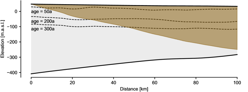
In order to define the inflow boundary condition, we would need to know the relative thickness of the incoming layers (or alternatively, the vertical age distribution at ). This is typically not available in radar measurements of the stratigraphy. It is therefore important to use only the IRH elevation information within the Local Meteoric Ice (LMI) body of the flow line. This is the region of our domain which is independent of the boundary condition we chose at (Fig. 10). This region can be found by tracking the trajectory traced by a particle initially at . The LMI body is the region of the domain above this path. As a consequence of this consideration, we need to discard more of the IRH elevation data for the deeper IRHs in the dataset.
For a complete definition of the simulator, we still need to define some boundary condition at . Since the true boundary condition is not known, we choose an inflow boundary condition which improves the numerical stability of the layer tracing model,
This boundary condition makes the implicit assumption that near the inflow boundary, the layer thickness profile is a scalar multiple of the total thickness,
We define a similar boundary condition at , however this boundary condition does not have a similar effect on the applicability of the IRH data.
Appendix B Calibrating the Simulator
We calibrate hyperparameters of the noise model using a set of 1000 simulations for the same ice shelf geometry, velocity, and mass balance parameters prior. This set of calibration simulations is not used again to train NPE (Sec. 2.2.1), to avoid overfitting. We use the same set of calibration simulations to calibrate the per-layer LMI boundary mask (Sec. 2.2.2).
B.1 Noise Distribution
Algorithm 1 defines our calibration procedure for the parameters of the noise distribution for Ekström Ice Shelf.
B.2 Boundary of LMI Body
In Sec. 2.2 we used the LMI boundary for each IRH in order to define the domain on which we compare the observed IRH data to the simulated isochronal layers. The physical interpretation of the LMI boundary is found in appendix A.2 , and here we specify the exact definition of .
For each simulation in the calibration set, we define the trajectory of a particle starting at the surface of the inflow boundary by . In practice, since we are on a flow line, everywhere, and thus increases monotonically with . Therefore the trajectory traces out a unique curve in the domain.
Using this path we define the LMI boundary for simulation and IRH to be the first point in the domain such that the path is below the IRH elevation,
In the case that the path stays above the IRH for the entire domain, we define , meaning that the IRH is entirely outside the LMI body.
This definition gives a different LMI body for each simulation. In order to perform inference, we require one a fixed LMI body boundary to use across all simulations. We define ”pessimistically” as the percentile of the calculated boundaries in the calibration set. Therefore, some of the simulated layer elevations we use will be dependent on the unknown boundary conditions, but a small amount that should not affect the inferred results.
Appendix C Implementation Details
For completeness we give the values of the important hyperparameters involved in the workflow - these are also explicit in the provided code repository.
C.1 Ice Flow Model
We provide the details of the spatial and temporal resolutions of our various simulations, along with the regularization strengths of the smoothing of the Ekström Ice Shelf data (Tables 1,2,3).
| Parameter | Value |
|---|---|
| mesh resolution | (310 \unitm, 250 \unitm) |
| spinup duration | 1000 years |
| spinup timestep | 1.0 years |
| Boundary Conditions | Dirichlet inflow and side boundaries |
| Parameter | Value |
|---|---|
| mesh resolution | 300 \unitm |
| Thickness smoothness reg. penalty | 1000 |
| Log fluidity reg. penalty | 1000 |
| Boundary Conditions | Dirichlet inflow and side boundaries |
| Parameter | Value |
|---|---|
| simulation time | 1000 years |
| time step | 0.5 years |
C.2 Network Architecture and Training
We applied Neural Posterior Estimation (NPE) as implemented in the sbi package [Tejero-Cantero \BOthers. (\APACyear2020)] to obtain the results for both the synthetic (Section 3) and Ekström (Section 4) ice shelves. We used the Neural Spline Flow (NSF) [Durkan \BOthers. (\APACyear2019)] as implemented in \citeALueckmann2021, and with the same network architecture as the NPE experiment. We also embedded the 500-dimensional observation of layer elevations to a 50-dimensional summary statistic used as the condition for the NSF. The embedding network consisted of two convolutional layers with kernel size 5, each followed by ReLU activations and max pooling with kernel size 2. The number of output channels for the two convolutional layers were 6 and 12 respectively. The output channels of the second convolutional layer were then concatenated and fed through two fully connected linear layers, each followed by ReLU activations. The number of hidden units was set to 50. Training was done as in \citeALueckmann2021, with the exception that the batch size was set to 1000 (default is 50). For each NPE run, we train 5 networks initialized with different random seeds, and report in our results the run with the best validation loss.
Appendix D Computational Costs
We provide a breakdown of the approximate computational costs of the different stages in our workflow for both synthetic and Ekström Ice Shelves in Tables 4 and 5 respectively. These are dependent the hardware used, and vary stochastically as a result of random number generators. This section is intended to provide intuition into the relative scales of the different stages of the workflow, rather than exact measurements. We had access to 16-core Intel Xeon Gold 2.9 GHz CPU nodes, and Nvidia RTX 2080ti GPU nodes. While the large number evaluations of the forward layer tracing model was by far the most computationally-intensive section of the workflow in both cases, these simulations were trivially performed in parallel across CPU cores, thus reducing the wall-clock time of the workflow.
This analysis highlights the advantages of our amortized approached to inference. For Ekström Ice Shelf, the total computational time of the noiseless simulations accounted for of the total computational time of the workflow. The simulations need not be repeated when we infer from other IRHs, greatly benefiting the computational efficiency of inference as the number of IRHs in the dataset increases. This advantage is slightly reduced when considering the parallelization we have used (Table 5), as the training of the probability density estimator is not easily parallelizable across GPU nodes. Accounting for this still results in of the computational cost being amortized.
| Task | Node [parallel] | Time [parallel] |
|---|---|---|
| Spin up of ice shelf | CPU | 120 |
| 1,000 calibration simulations | CPU [100 cores] | 1000 [10] |
| 189,000 noiseless simulations | CPU [100 cores] | [2000] |
| Noise and layer selection | CPU [100 cores] | 400 [20] |
| Training NPE for 1 IRH | GPU | 30 |
| Only the last two tasks need to be repeated for each IRH measurement. | ||
| Task | Node [parallel] | Time [parallel] |
| Generating Mesh | CPU | |
| Data preprocessing | CPU | 10 |
| 1,000 calibration simulations | CPU [100 cores] | 1000 [10] |
| 189,000 noiseless simulations | CPU [100 cores] | [2000] |
| Noise and layer selection | CPU [100 cores] | 400 [20] |
| Training NPE for 1 IRH | GPU | 30 |
| Only the last two tasks need to be repeated for each IRH measurement. | ||
Appendix E Additional Results
E.1 Synthetic Ice Shelf
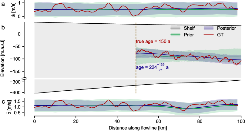
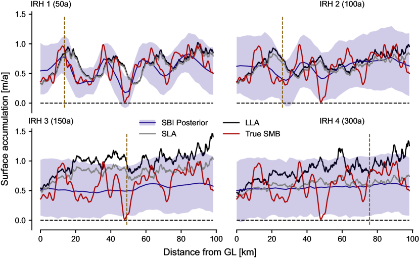
We show the posterior and posterior predictive distributions when inferring from isochronal layer 3 in the synthetic ice shelf dataset, of age 150 years (Fig. 11. This isochronal layer has average depth of 120 \unitm, comparable to the deepest IRH in the Ekström dataset. While the uncertainty is much higher than for the shallow layer, the posterior over the surface accumulation still shows a higher mean than the prior in the downstream section of the ice shelf. Additionally, the posterior predictive reconstructs the ground truth isochronal layer better than the prior predictive. The mean root mean square error (RMSE) of the posterior predictive layers relative to the ground truth is 13.6 \unitm, compared to 19.8 \unitm for the prior. Therefore we are still able to reconstruct additional information about the mass balance parameters, even from much deeper layers.
We also explore the dependence of the inferred posterior over surface accumulation rate on the depth of the layer used for inference in the synthetic case (Fig. 12), similar to the analysis done in Section 5.2 for Ekström Ice Shelf. For the synthetic ice shelf, the surface accumulation and basal melt rates were held constant for the entire simulation time, and hence the increased uncertainty with depth seen in Fig. 12 highlights that information about the mass balance parameters is gradually lost with time as a result of the action of the simulator. Indeed, for the deepest ground truth isochronal layer of average depth 183 \unitm, the posterior distribution is almost identical to the prior distribution.
E.2 Error in Predictive Distributions
Here we report the Root Mean Square Error (RMSE) in the predicted isochronal layer elevations, relative to the true IRH (for Ekström Ice Shelf) or the ground truth isochronal layer (for the synthetic ice shelf). This is done across simulations from 1000 simulations for each of the prior and posterior distributions, for each IRH. The RMSE is consistently lower for the posterior predictive distribution for all depths, for both the synthetic ice shelf (Table 6) and Ekström Ice Shelf (Table 7).
| prior | posterior | |||
|---|---|---|---|---|
| IRH number | RMSE mean | RMSE SD | RMSE mean | RMSE SD |
| 1 | 11.5 | 3.9 | 3.9 | 0.5 |
| 2 | 16.0 | 7.6 | 7.3 | 1.2 |
| 3 | 19.8 | 8.4 | 13.6 | 3.5 |
| 4 | 22.1 | 7.9 | 19.8 | 6.8 |
| prior | posterior | |||
|---|---|---|---|---|
| IRH number | RMSE mean | RMSE SD | RMSE mean | RMSE SD |
| 1 | 6.8 | 2.1 | 3.0 | 0.9 |
| 2 | 11.8 | 3.4 | 4.6 | 1.3 |
| 3 | 17.0 | 6.6 | 6.8 | 1.4 |
| 4 | 16.4 | 7.6 | 10.0 | 2.1 |
Appendix F Kottas Traverse Data
Here we describe the mapping of the surface accumulation measurements on Kottas traverse to the flow line transect. For each measurement year, and each location on the Kottas traverse, we find the nearest point on the flow line transect. We assume the accumulation rate at this point to be normally distributed, with mean (the Kottas traverse measurement at ), and variance . We set the length scale \unitkm and the accumulation rate variance \unitm^2\unita^-2. These values are chosen in accordance to the definition of the surface accumulation rate prior distribution (Sec. 2.2.3).
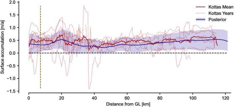
The yearly variations of the estimated surface accumulation as measured using the stake line along the Kottas traverse (Fig. 13 reasonably agree with the posterior inferred using IRH 2 (Section 4.1). These show that there is a high year-to-year variability in the surface accumulation (\citeAMengert2018, Fig. 13) even in this steady-state region in East Antarctica. However, the mean of these yearly measurements matches the inferred posterior mean closely.
Appendix G Synthetic Results with Miscalibrated Prior
An additional outcome of our approach is the estimation of the age of isochronal layers. However, the validity of this estimate depends on the prior distribution containing the true mass balance parameters. When the true mass balance parameters have low probability under the prior distribution, the resulting estimate for the age of the isochronal layer can be wrong. We test this on the synthetic ice shelf by choosing a ground truth surface accumulation that has low probability under the prior distribution. We calculate the isochronal layer of age 100 years under this ground truth and obtain the posterior distribution as before, using the same set of simulations as in the main text. The posterior does not capture that the mean surface accumulation rate should be higher than what is defined in the prior (Fig. 14a). However, this is not a failure of the inference method, as we can see that the posterior predictive still reconstructs the ground truth isochronal layer at higher fidelity than the prior (Fig. 14b). The predicted age of the isochronal layer years, which greatly overestimates the true age of 100 years.