Exploring the nonclassical dynamics of the “classical” Schrödinger equation

Abstract

The introduction of nonlinearities in the Schrödinger equation has been considered in the literature as an effective manner to describe the action of external environments or mean fields. Here, in particular, we explore the nonlinear effects induced by subtracting a term proportional to Bohm’s quantum potential to the usual (linear) Schrödinger equation, which generates the so-called “classical” Schrödinger equation. Although a simple nonlinear transformation allows us to recover the well-known classical Hamilton-Jacobi equation, by combining a series of analytical results (in the limiting cases) and simulations (whenever the analytical treatment is unaffordable), we find an analytical explanation to why the dynamics in the nonlinear “classical” regime is still strongly nonclassical. This is even more evident by establishing a one-to-one comparison between the Bohmian trajectories associated with the corresponding wave function and the classical trajectories that one should obtain. Based on these observations, it is clear that the transition to a fully classical regime requires extra conditions in order to remove any trace of coherence, which is the truly distinctive trait of quantum mechanics. This behavior is investigated in three paradigmatic cases, namely, the dispersion of a free propagating localized particle, the harmonic oscillator, and a simplified version of Young’s two-slit experiment.

1 Introduction

Typically, the emergence of the classical world from the quantum one is associated with the action of decoherence [1, 2, 3, 4, 5]. Accordingly, the constant interaction with an environment is what eventually leads a given (quantum) system of interest to loose its quantumness (its ability to display genuine quantum features, such as interference, for instance), and hence to behave like the objects that we observe in our everyday life. The theory of open quantum systems [6] contains a wide variety of effective models to investigate the effects and consequences arising from the environmental interaction, while avoiding the technical complexities (analytical and numerical) inherent to the corresponding many-body problems. Among all such models, the Lindblad equation provides us with the most general form of a master equation, where the environmental action on the system reduced density matrix is described by a dissipator term. Nonetheless, if we are interested in a wave-function based description, still the Lindblad equation can be recast in terms of a stochastic nonlinear equation, according to the quantum state diffusion approach [7, 8, 9].

To investigate the quantum-to-classical transition, however, there is an alternative route, which consists in considering effective nonlinear equations. This is the case of the so-called “classical” Schrödinger equation,

$$i\hbar\frac{\partial\psi({\bf r},t)}{\partial t}=-\frac{\hbar^{2}}{2m}\nabla^{2}\psi({\bf r},t)+V({\bf r})\psi({\bf r},t)+\frac{\hbar^{2}}{2m}\frac{\nabla^{2}A({\bf r},t)}{A({\bf r},t)}\psi({\bf r},t),$$ (1)

where the effect of introducing a nonlinear term on the right-hand side gives rise to a phase dynamics governed by a classical-like Hamilton-Jacobi equation. Concerning this addition, it is worth noting that the introduction of nonlinear terms into the Schrödinger equation has been considered in the literature as an effective manner to recover or reproduce classical-like behaviors. For instance, the Kostin or Schrödinger-Langevin equation [10, 11, 12] or the Schuch-Chung-Hartmann equation [13, 14, 15] constitute attempts to describe dissipation in a pure quantum state, in an analogous manner to how it is done in classical mechanics, with a friction term. In the first case, in particular, the dissipative term is associated with the phase of the wave function, while in the latter it is related to the square of its amplitude (i.e., the probability density). The so-called Schrödinger-Newton equation is another example of effective nonlinear equation, formerly intended to investigate the equilibrium configurations of self-gravitating systems of scalar bosons and spin$-1/2$ fermions, and later reconsidered to study the role of gravity in the collapse of the wave function (the so-called problem of the quantum state reduction) and, therefore, how classicality emerges in a cosmological scenario [16, 17].

Following the Van Vleck semiclassical formulation of quantum mechanics [18], Schiller found [19] that by modifying the classical Hamilton-Jacobi equation one can obtain a classical Schrödinger equation with classical complex-valued wave functions. Almost by the same time, Rosen also found the same equation while investigating when quantum and classical dynamics look the same [20, 21, 22, 23]. A heuristic derivation of this equation employing the language of Lagrangian dynamics is given by Holland [24], who also discusses a series of aspects related to it and its solutions concerning the dissimilarities between quantum and classical motions (“classical” in terms of this nonlinear equation). More recently, it has also been revisited by Schleich et al. [25], from whom “the linearity of quantum mechanics is intimately connected to the strong coupling between the amplitude and phase of a quantum wave”, which is, actually, what the Bohm’s picture of quantum mechanics emphasizes. On the other hand, numerical simulations of well-known paradigmatic quantum systems carried out by Chou [26, 27] and Benseny et al. [28] show that, despite of the strong connection between the classical Schrödinger equation and the classical Hamilton-Jacobi, there are still major discrepancies between the motions generated by one and the other.

To better understand what really makes interesting the classical Schrödinger equation, it is worth noting the fact that it includes a locally evaluated mean or self-consistent field term that antagonizes the dispersive contribution implicit in the kinetic operator. Thus, like Schiller [19], let us consider the system wave function in polar form,

$$\psi({\bf r},t)=A({\bf r},t)e^{iS({\bf r},t)/\hbar},$$ (2)

where both $A({\bf r},t)=\sqrt{\rho({\bf r},t)}$ and $S({\bf r},t)$ are real-valued fields describing, respectively, the local variations of the probability amplitude (or the probability density $\rho$) and the phase undergone by the system. The action of the kinetic operator, $\hat{\mathcal{K}}=-(\hbar^{2}/2m)\nabla^{2}$, on this ansatz, divided by $\psi({\bf r},t)$, produces

$$\frac{\hat{\mathcal{K}}\psi({\bf r},t)}{\psi({\bf r},t)}=\frac{[\nabla S({\bf r},t)]^{2}}{2m}-\frac{\hbar^{2}}{2m}\frac{\nabla^{2}A({\bf r},t)}{A({\bf r},t)}-\frac{i\hbar}{2}\frac{\nabla{\bf j}({\bf r},t)}{\rho({\bf r},t)}\ .$$ (3)

On the right-hand side of the above equation, we have

$${\bf j}({\bf r},t)=\rho({\bf r},t){\bf v}({\bf r},t)=\frac{1}{m}\ {\rm Re}\left[\psi^{*}({\bf r},t)\hat{\bf p}\psi({\bf r},t)\right],$$ (4)

which is the usual quantum flux [29], where $\hat{\bf p}=-i\hbar\nabla$ is the usual momentum operator, and

$${\bf v}({\bf r},t)=\frac{{\bf j}({\bf r},t)}{\rho({\bf r},t)}=\frac{1}{m}\ {\rm Im}\left[\frac{\hat{\bf p}\psi({\bf r},t)}{\psi({\bf r},t)}\right]=\frac{\nabla S({\bf r},t)}{m}$$ (5)

is a velocity field that accounts for the local phase variations. Within the context of Bohmian mechanics, this velocity field is directly related to the so-called Bohm’s momentum [30].

From a physical point of view, the three terms in Eq. (3) contribute to a different dynamical aspect displayed by the wave function during its evolution [31]. The imaginary term, which depends on the quantum flux and the probability density, is related to the conservation of the latter. As for the two real-valued contributions, they are specifically related to the wave function propagation dynamics. In analogy to the role of the kinetic term within the classical Hamilton-Jacobi formulation, the first one of these contributions is also a purely kinetic term, i.e., it is connected to the “motion” of the wave function in the corresponding configuration space. However, because a wave function is an extensive object, its dynamics is also strongly influenced by its own configuration, which is precisely what the second term accounts for, as it depends on the local changes undergone by the amplitude of the wave function (more specifically, it is a measure of its local curvature at a given time $t$). In the literature, this term is the so-called Bohm’s quantum potential [30, 32, 24], although the term “potential” might be certainly misleading, as neither its origin nor its action on the system have to do with those of a usual potential function. Note that it is responsible for dispersion or diffraction of the wave function, thus governing its spreading [31, 33].

The idea of a classical Schrödinger equation thus departs from the above considerations: if an anti-quantum potential term is added to the usual Schrödinger equation, then it should counteract the dispersive effects induced by the quantum potential generated by the kinetic operator and, therefore, the dynamics displayed by the quantum system should look pretty much like classical dynamics, since only the classical-like contribution, $(\nabla S)^{2}/2m$, remains. The purpose in this work is to investigate this conjecture, which, in principle, seems to solve the problem of the classical limit and the quantum-classical correspondence, as trajectories can also be introduced in quantum mechanics through Eq. (5). Specifically, by integrating in time the equation of motion $\dot{\bf r}={\bf v}({\bf r},t)$, we obtain the so-called Bohmian trajectories in a natural manner [34], which here are interpreted as paths or streamlines that serve to monitor the flux of the probability density [35] rather than the actual paths followed by real particles. Note that, if the polar ansatz (2) is substituted into the nonlinear Schrödinger equation (1), we obtain

$$-\frac{\partial S({\bf r},t)}{\partial t} = \frac{[\nabla S({\bf r},t)]^{2}}{2m}+V({\bf r}),$$ (6)

$$\frac{\partial\rho({\bf r},t)}{\partial t} = -\nabla{\bf j}({\bf r},t),$$ (7)

where Eq. (7) is the continuity equation, while Eq. (6) looks like a classical Hamilton-Jacobi equation.

Unlike previous works [26, 27, 28], here we are interested in providing analytical solutions to also paradigmatic cases in order to better understand the main differences between the quantum (Bohmian) solutions and the classical ones, and, more specifically, such differences come from. In particular, the analysis will focus on some paradigmatic systems, such as dispersion of a free particle, the harmonic oscillator, or two-wave packet interference, as all of them capture in one way or another the essence of what we understand by non-classical behavior in a simple manner, even though they are often invoked to explain more complex problems. To tackle the issue, we revisit the transition from a fully quantum or linear regime, described by the usual Schrödinger equation, to the (seemingly) classical one determined by the nonlinear Eq. (1) by adding a coupling factor, $\lambda$, to the nonlinearity. This coupling factor ranges from 0 to 1, which allows us to pass from the linear to the nonlinear case in a smooth manner. To proceed in an analytical manner in as much as possible, at least, in the limiting cases, we have considered Heller’s frozen Gaussian wave-packet method [36]. According to this method, the propagation of a Gaussian wave packet can be determined by means of a a series of time-dependent parameters that obey a set of coupled ordinary differential equations, to which the Bohmian equation of motion can also be added [33], which acquires a rather simple form. In some particular instances, these equations admit analytical solutions, which makes the interpretation of the corresponding dynamics more evident, even in those cases where the wave function consists of coherent superpositions of such wave packets and the full solution is no longer analytical. Thus, the results obtained show that, although the overall classical behaviors are nicely reproduced, there are still major differences that avoid us to speak about a true classical limit, in agreement with previously reported data. In this regard, even though a classical-like equation is recovered from the nonlinear Schrödinger equation (1), the dynamics still keeps strong non-classical features.

The organization of this work is as follows. In next section, we briefly introduced the equations of motion in the general case. The dynamics for single wave packets is discussed in Sec. 3, considering both free propagation and the harmonic oscillator. In Sec. 4 we present results for two wave-packet interference propagating both in free space and inside a harmonic potential. Finally, the main conclusions extracted from this work are presented in Sec. 5.

2 General framework

For simplicity, let us consider the case of a one-dimensional non-relativistic particle with mass $m$ acted by the nonlinear Schrödinger equation

$$i\hbar\frac{\partial\psi(x,t)}{\partial t}=-\frac{\hbar^{2}}{2m}\frac{\partial^{2}\psi(x,t)}{\partial t^{2}}+V(x)\psi(x,t)+\lambda\ \frac{\hbar^{2}}{2m}\frac{1}{A(x,t)}\frac{\partial^{2}A(x,t)}{\partial x^{2}}\ \psi(x,t),$$ (8)

where the potential function $V(x)$ can be recast as a second-degree polynomial (higher order polynomials are disregarded here because of their loss of analyticity, as discussed below) and the parameter $\lambda$ determines the strength of the coupling with the nonlinear contribution, with its value ranging between 0 (linear regime) and 1 (classical regime). Regardless of the nonlinear term, the equation of motion for the trajectories describing the time evolution of systems governed by Eq. (8) is

$$\dot{x}(x,t)=\frac{j(x,t)}{\rho(x,t)}=\frac{1}{m}\frac{\partial S(x,t)}{\partial x}.$$ (9)

Given the degree of the potential, let us then consider the suitable Gaussian ansatz

$$\psi(x,t)=e^{i\alpha_{t}(x-x_{t})^{2}/\hbar+i\beta_{t}(x-x_{t})/\hbar+i\gamma_{t}/\hbar}.$$ (10)

which depends on the parameters $\alpha_{t}$, $\beta_{t}$, $\gamma_{t}$, and $x_{t}$. The justification for this ansatz arises [36] from the fact that, if the wave packet is sufficiently narrow for a time and it is acted by a relatively smooth external potential, then the dynamics of such a wave packet will only be affected (for such a time duration) by the first terms in the Taylor expansion of the potential around its centroidal position, according to Ehrenfest’s theorem [29]. That is, if we retain terms up to $(x-x_{t})^{2}$ in this Taylor expansion, then the wave packet will be acted, in good approximation, by a harmonic potential, which means that initially Gaussian wave packets will preserve their Gaussian shape.

The ansatz (10) allows us to obtain the solutions to the nonlinear Schrödinger equation (8) from a set of partial differential equations instead of solving directly a nonlinear partial differential equation. Those equations arise after substituting (10) into Eq. (8), with the corresponding approximation, up to second order, for the potential function around $x_{t}$, i.e.,

$$V(x,t)=V_{t}(x_{t})+V^{\prime}_{t}(x_{t})(x-x_{t})+\frac{1}{2}\ V^{\prime\prime}_{t}(x_{t})(x-x_{t}),$$ (11)

and then separating in terms of the powers of $(x-x_{t})$. Moreover, let us also consider a series of conditions that simplify the calculations. From the normalization condition for the ansatz (10), we obtain a relationship between the imaginary parts of $\alpha_{t}$ and $\gamma_{t}$:

$$\gamma^{i}_{t}=-\frac{\hbar}{4}\ \ln\left[\frac{2\alpha^{i}_{t}}{\pi\hbar}\right],$$ (12)

where a superscript “i” is used to denote imaginary part (similarly, a superscript “r” will be used to label the real part of a quantity from now on). Since the condition (12) must be satisfied at any time and, at $t=0$ it implies the initial condition

$$\gamma^{i}_{0}=-\frac{\hbar}{4}\ \ln\left[\frac{2\alpha^{i}_{0}}{\pi\hbar}\right].$$ (13)

On the other hand, taking into account (12), if we compute the expectation value for the position and momentum of (8), we obtain

$$\langle\hat{x}\rangle=x_{t},\qquad\langle\hat{p}\rangle=\beta_{t}.$$ (14)

Accordingly, both $x_{t}$ and $\beta_{t}$ are real-valued quantities, which determine the instantaneous position and momentum of the centroid of the wave packet centroid in phase space.

Proceeding now as it was indicated above, we obtain, respectively, from the zeroth, first, and second orders in $(x-x_{t})$ the following equations

$$\dot{\gamma}_{t} = \frac{i\hbar\alpha_{t}}{m}+\beta_{t}\dot{x}_{t}-\frac{\beta_{t}^{2}}{2m}+V_{t}+\frac{\lambda\hbar}{m}\ \alpha^{i}_{t}-\frac{\lambda}{2m}\left(\beta^{i}_{t}\right)^{2},$$ (15)

$$2\alpha_{t}\left(\dot{x}_{t}-\frac{\beta_{t}}{m}\right) = \dot{\beta}_{t}+V^{\prime}_{t}+\frac{2\lambda\hbar}{m}\ \alpha^{i}_{t}\beta^{i}_{t},$$ (16)

$$\dot{\alpha}_{t} = -\frac{2\alpha_{t}^{2}}{m}-\frac{1}{2}\ V^{\prime\prime}_{t}-\frac{2\lambda}{m}\left(\alpha^{i}_{t}\right)^{2}.$$ (17)

Because $\beta_{t}$ is real, according to (14), Eq. (16) reduces to

$$2\alpha_{t}\left(\dot{x}_{t}-\frac{\beta_{t}}{m}\right)=\dot{\beta}_{t}+V^{\prime}_{t}.$$ (18)

Now, since $\alpha_{t}$ is complex and the right-hand side of Eq. (18) is real, the following identities must be satisfied:

$$\dot{x}_{t}=\frac{\beta_{t}}{m},\qquad\dot{\beta}_{t}=-V^{\prime}_{t},$$ (19)

which is in compliance with Ehrenfest’s theorem, i.e., the centroid of the wave packet evolves in time according to the classical Hamiltonian equations, with $x_{t}$ and $p_{t}$ defining a classical trajectory. Thus, from now on, we will denote $\beta_{t}$ as $p_{t}$. Accordingly, Eq. (15) can be recast in a simpler manner, as

$$\dot{\gamma}_{t}=\frac{i\hbar\alpha_{t}}{m}+p_{t}\dot{x}_{t}-E_{t}+\frac{\lambda\hbar}{m}\ \alpha_{t},$$ (20)

where $E_{t}=p_{t}^{2}/2m+V_{t}$.

Therefore, the set of equations of motion that determine the time evolution of the ansatz wave function (8) is

$$\dot{x}_{t} = \frac{p_{t}}{m},$$ (21)

$$\dot{p}_{t} = -V^{\prime}_{t},$$ (22)

$$\dot{\alpha}^{r}_{t} = -\frac{2(\alpha^{r}_{t})^{2}}{m}+(1-\lambda)\ \frac{2(\alpha^{i}_{t})^{2}}{m}-\frac{1}{2}V^{\prime\prime}_{t},$$ (23)

$$\dot{\alpha}^{i}_{t} = -\frac{4\alpha^{r}_{t}\alpha^{i}_{t}}{m},$$ (24)

$$\dot{\gamma}^{r}_{t} = -(1-\lambda)\ \frac{\hbar\alpha^{i}_{t}}{m}+p_{t}\dot{x}_{t}-E_{t},$$ (25)

$$\dot{\gamma}^{i}_{t} = \frac{\hbar\alpha^{r}_{t}}{m}.$$ (26)

To this set of equations, we need to add the general expression for the equation of motion of the trajectories, which reads as [33]

$$\dot{x}=\frac{1}{m}\left[p_{t}+2\alpha^{r}_{t}(x-x_{t})\right].$$ (27)

The trajectories obtained from this equation for each case will help us to understand the role played by the anti-quantum potential in terms of the coupling strength $\lambda$. Note that, if $\lambda=0$, the above system of equations reproduces the original Heller’s set [36, 33], while for $\lambda=1$, the real part of both $\alpha_{t}$ and $\gamma_{t}$ decouples from the imaginary part of $\alpha_{t}$, which is related to the dispersion of the wave packet. This is better appreciated if Eq. (27) is recast as

$$\frac{\dot{x}-p_{t}/m}{x-x_{t}}=\frac{2\alpha^{r}_{t}}{m},$$ (28)

which can readily be integrated to yield the general expression

$$x(t)=x_{t}+\left[x(0)-x_{0}\right]e^{\int_{0}^{t}2\alpha^{r}_{t^{\prime}}/m\ dt^{\prime}}.$$ (29)

Accordingly, any effect induced by $\alpha^{i}_{t}$ on the Bohmian trajectories disappears, as Eq. (27) will only depend on $\alpha^{r}_{t}$. On the other hand, the phase accumulated by the wave, accounted for by $\gamma^{r}_{t}$, will equal the classical action, $\mathcal{S}=\int\mathcal{L}\ dt$, where $\mathcal{L}=p_{t}\dot{x}_{t}/2-V_{t}$ is the classical Lagrangian.

3 Single wave packet dynamics

3.1 Free-space propagation

In the case of free-space propagation, $V(x)=0$, the set of equations (21)-(26) becomes

$$\dot{x}_{t} = \frac{p_{t}}{m},$$ (30)

$$\dot{p}_{t} = 0,$$ (31)

$$\dot{\alpha}^{r}_{t} = -\frac{2(\alpha^{r}_{t})^{2}}{m}+(1-\lambda)\ \frac{2(\alpha^{i}_{t})^{2}}{m},$$ (32)

$$\dot{\alpha}^{i}_{t} = -\frac{4\alpha^{r}_{t}\alpha^{i}_{t}}{m},$$ (33)

$$\dot{\gamma}^{r}_{t} = -(1-\lambda)\ \frac{\hbar\alpha^{i}_{t}}{m}+p_{t}\dot{x}_{t}-E_{t},$$ (34)

$$\dot{\gamma}^{i}_{t} = \frac{\hbar\alpha^{r}_{t}}{m}.$$ (35)

If the initial ansatz is

$$\psi(x,0)=\left(\frac{1}{2\pi\sigma_{0}^{2}}\right)^{1/4}e^{-(x-x_{0})^{2}/4\sigma_{0}^{2}+ip_{0}(x-x_{0})},$$ (36)

we have the following initial conditions for the Gaussian parameters:

$$\alpha_{0}=\frac{i\hbar}{4\sigma_{0}^{2}},\qquad\gamma_{0}=\frac{i\hbar}{4}\ \ln\left(2\pi\sigma_{0}^{2}\right),$$ (37)

and $(x_{0},p_{0})$ for $(x_{t},p_{t})$. For the linear case, the solutions are readily obtained, being

$$x_{t} = x_{0}+\frac{p_{0}}{m}\ t,$$ (38)

$$p_{t} = p_{0},$$ (39)

$$\alpha_{t} = \frac{i\hbar}{4\sigma_{0}^{2}}\left(\frac{1}{1+i\hbar t/2m\sigma_{0}^{2}}\right)=-\frac{i\hbar}{4\sigma_{0}\tilde{\sigma}_{t}},$$ (40)

$$\gamma_{t} = \gamma_{0}+\frac{i\hbar}{2}\ \ln\left(1+\frac{2\alpha_{0}t}{m}\right)=\frac{i\hbar}{4}\ \ln\left(2\pi\tilde{\sigma}_{t}\right),$$ (41)

where

$$\tilde{\sigma}_{t}=\sigma_{0}\left(1+\frac{i\hbar t}{2m\sigma_{0}^{2}}\right).$$ (42)

We thus obtain the usual Gaussian dispersion or diffraction, described by the wave function

$$\psi(x,t)=\left(\frac{1}{2\pi\tilde{\sigma}_{t}^{2}}\right)^{1/4}e^{-(x-x_{0})^{2}/4\sigma_{0}\tilde{\sigma}_{t}+ip_{0}(x-x_{t})/\hbar-E_{t}t/\hbar},$$ (43)

and the typical hyperbolic trajectories describing these dynamics,

$$x(t)=x_{t}+\frac{\sigma_{t}}{\sigma_{0}}\left[x(0)-x_{0}\right],$$ (44)

where

$$\sigma_{t}=|\tilde{\sigma}_{t}|=\sigma_{0}\sqrt{1+\left(\frac{\hbar t}{2m\sigma_{0}^{2}}\right)^{2}}.$$ (45)

The above results and their dynamical consequences are well-known (see Refs. [31, 33] for a general discussion). In order to better understand the physics associated with the $\alpha_{t}$-parameter as well as its contribution to the quantumness of the system, we now consider a more general initial condition $\alpha_{0}$, such that $\alpha^{r}_{0}\neq 0$. In this case, the integration in time of Eqs. (32) and (33) renders

$$\alpha_{t}=\frac{\alpha_{0}}{1+2\alpha_{0}t/m},$$ (46)

where its real part being

$$\alpha^{r}_{t}=\frac{\alpha^{r}_{0}}{1+(2|\alpha_{0}|t/m)^{2}}+\frac{2|\alpha_{0}|^{2}t/m}{1+(2|\alpha_{0}|t/m)^{2}}.$$ (47)

Substituting Eq. (47) into Eq. (29), and then integrating in time, yields

$$x(t)=x_{t}+\frac{\sigma_{t}}{\sigma_{0}}\left[x(0)-x_{0}\right]e^{(\alpha^{r}_{0}/|\alpha_{0}|)\ \tan^{-1}(2|\alpha_{0}|t/m)}.$$ (48)

According to this expression, a non-vanishing contribution of the real part of $\alpha_{t}$ introduces changes in the shape displayed by the trajectories of a free-propagating wave packet, even without the presence of an external potential. Specifically, these changes consist in a faster or a slower spreading, depending on whether the sign of $\alpha^{r}_{0}$ is positive or negative, respectively. Moreover, this also introduces an asymmetry in the propagation with respect to $t=0$, noting that, for positive $\alpha^{r}_{0}$, the spreading will approach $t=0$ (from $-\infty$) at a slower rate, while for negative $\alpha^{r}_{0}$, the spreading will reduce more drastically, at a faster rate.

With respect to the other limiting case, namely, the full nonlinear scenario, with $\lambda=1$, the initial conditions (37) lead to

$$\alpha_{t} = \frac{i\hbar}{4\sigma_{0}^{2}},$$ (49)

$$\gamma_{t} = \frac{i\hbar}{4}\ \ln\left(2\pi\sigma_{0}\right),$$ (50)

and, therefore, the “classical” wave function will read as

$$\psi(x,t)=\left(\frac{1}{2\pi\sigma_{0}^{2}}\right)^{1/4}e^{-(x-x_{t})^{2}/4\sigma_{0}^{2}+ip_{0}(x-x_{t})-iEt/\hbar}.$$ (51)

This wave function is very similar to the wave function (43), except for the lack of a dispersive term, since its width is constant in time, as one might expect once the dispersive contribution accounted for by $\alpha_{t}^{i}$ is suppressed. This gives rise to the phenomenon of spatial localization, which is precisely the behavior that one would expect for a free-propagating Gaussian classical statistical particle distribution, where all its constituents (an ensemble of identical, non-interacting particles) have exactly the same momentum $p_{0}$. Accordingly, given that the phase factor is linear in the position, the Bohmian trajectories will be straight lines described by the equation

$$x(t)=x(0)+\frac{p_{0}}{m}\ t,$$ (52)

as it corresponds to uniform motion.

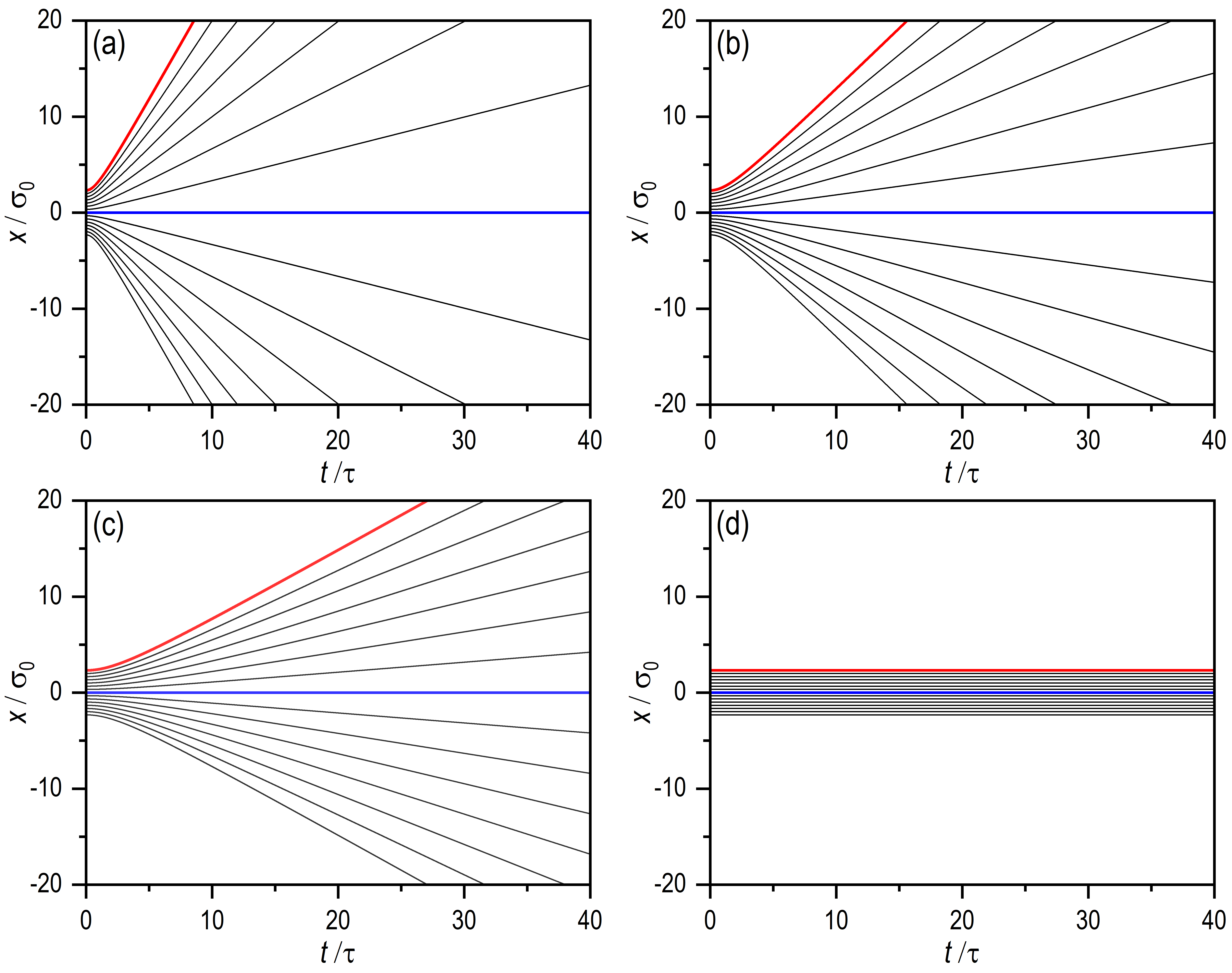
Figure 1: Suppression of the dispersion of a single Gaussian wave packet with an initial width $\sigma_{0}=$ and increasing coupling constant: (a) $\lambda=0$, (b) $\lambda=0.7$, (c) $\lambda=0.9$, and (d) $\lambda=1$. A set of 15 Bohmian trajectories has been used to illustrate the process and, in turn, to show how these trajectories eventually show a classical-like behavior, in the Newtonian sense, for $\lambda=1$ in panel (d). The initial conditions for these trajectories are such that the blue trajectory has been launched from the center of the wave packet, while the red one starts at a $2.5\sigma_{0}$-distance from it. In all simulations here, we have considered $\hbar=1$, $m=1$, $\sigma=0.5$, $x_{0}=0$, and $p_{0}=0$.

As we have seen, the classical wave function (51) is dispersionless and has a definite energy, $E$, which translates into Bohmian trajectories all with the same momentum. This results confirms the hypothesis that the quantum potential is directly responsible for dispersion or diffraction phenomena, since the rectilinear motion is unaffected. The four sets of trajectories plotted in Fig. 1 correspond to four different values of the strength coupling constant, $\lambda$, ranging from a full quantum regime to a full classical one: (a) $\lambda=0$, (b) $\lambda=0.7$, (c) $\lambda=0.9$, and (d) $\lambda=1$. These trajectories have been obtained by numerically integrating the set of coupled equations (30) to (35) together with Eq. (27). As it can be seen, the increase of $\lambda$ leads to a cancellation of the diffraction undergone by the wave packet. The trajectories represented with blue and red solid lines help to better visualize how, as $\lambda$ increases, the whole set approaches the dispersionless condition.

Usually, within the full quantum regime, an increase in $\sigma_{0}$ (or in the mass $m$) gives rise to slowing down the diffraction process, since the effective width of the wave packet, described by Eq. (45), becomes remains nearly constant ($\sigma_{t}\approx\sigma_{0}$) for longer times. The characteristic time that determines when diffractive effects are going to become apparent is

$$\tau=\frac{2m\sigma_{0}^{2}}{\hbar}.$$ (53)

However, the action of a non-vanishing anti-quantum potential generates an analogous inverse effect, as it annihilates the imaginary component in (42), which is equivalent to diminishing the relevance of the time scale $\tau$.

From the above results, it is thus clear that the presence of an anti-quantum potential nonlinear contribution in the Schrödinger equation leads to motions that, at least in appearance, are classical-like. This, however, does not constitute a proof itself of the classicality of the system in the regime $\lambda=1$. Note that, if we again consider a non-vanishing real part for $\alpha_{0}$, then the real and imaginary parts for $\alpha_{t}$ will read as

$$\alpha^{r}_{t} = \frac{\alpha^{r}_{0}}{1+2t\alpha^{r}_{0}/m},$$ (54)

$$\alpha^{i}_{t} = \alpha^{i}_{0}e^{-2\ln(1+2t\alpha^{r}_{0}/m)}$$ (55)

and, from Eq. (54), we obtain the trajectory equation

$$x(t)=x_{t}+\left(1+\frac{2t\alpha^{r}_{0}}{m}\right)[x(0)-x_{0}]=x(0)+\left\{\frac{p_{0}}{m}+\frac{2\alpha^{r}_{0}}{m}\ [x(0)-x_{0}]\right\}t,$$ (56)

which indicates that the trajectories will spread with a different rate depending on their distance with respect to the center of the wave packet, $x_{0}$, something that also happens in the fully linear regime ($\lambda=0$) for large $t$ [35].

Apart from the “non-classical” behavior that we have just found for a non-vanishing $\alpha^{r}_{t}$, an important distinctive trait of classical trajectories is that they can get across the same spatial point at the same instant, because of the multi-valuedness of the momentum. In the present context, therefore, this means that a genuine classical behavior should lead to a violation of the well-known Bohmian non-crossing rule [31]. To investigate this hypothesis, next we consider two scenarios that should help to prove it or disprove it, namely, the harmonic oscillator and the two wave-packet interference.

3.2 Harmonic oscillator

Consider a Gaussian wave packet acted by a harmonic potential,

$$V(x)=\frac{1}{2}\ m\omega^{2}x^{2}.$$ (57)

In the linear case ($\lambda=0$), the general solution to Heller’s equations (21) to (26) is

$$x_{t} = x_{0}\cos\omega t+\frac{p_{0}}{m\omega}\ \sin\omega t,$$ (58)

$$p_{t} = p_{0}\cos\omega t-m\omega x_{0}\sin\omega t,$$ (59)

$$\alpha_{t} = \frac{m\omega}{2}\frac{2\alpha_{0}/m\omega-\tan\omega t}{1+(2\alpha_{0}/m\omega)\tan\omega t},$$ (60)

$$\gamma_{t} = -\frac{i\hbar}{4}\ \ln\left(\frac{2\alpha^{i}_{0}}{\pi\hbar}\right)+\frac{i\hbar}{2}\ \ln\left(\cos\omega t+\frac{2\alpha_{0}}{m\omega}\sin\omega t\right)$$ (61)

$$+\frac{1}{2\omega}\left(\frac{p_{0}^{2}}{2m}-\frac{1}{2}\ m\omega^{2}x_{0}^{2}\right)\sin 2\omega t-p_{0}x_{0}\sin^{2}\omega t.$$

These solutions describe the dynamics of a “breathing” Gaussian wave packet, i.e., a wave packet with an oscillatory width as it propagates back and forth between the turning points of the potential function (57), $x_{\pm}=\pm\sqrt{2E/m\omega^{2}}$.

If we choose the initial condition $\alpha_{0}=im\omega/2\hbar$, from Eq. (60) we readily obtained that $\alpha_{t}=\alpha_{i}$, that is, the width of the wave packet is constant all the way down during its back and forth journey, with its wave function being

$$\psi(x,t) = \left(\frac{m\omega}{\pi\hbar}\right)^{1/4}e^{-(m\omega/2\hbar)(x-x_{t})^{2}}$$ (62)

$$\qquad\times e^{i[p_{t}x/\hbar-(p_{0}^{2}/2m-m\omega^{2}x_{0}^{2}/2)\sin 2\omega t/2\hbar\omega-p_{0}x_{0}\cos^{2}\omega t/\hbar-\omega t/2]},$$

which has a constant amplitude, because its width remains constant at any time, $\sigma_{0}=\sqrt{\hbar/2m\omega}$. Correspondingly, its space-dependent phase factor is linear with the $x$-coordinate, which gives rise to the trajectory equation

$$x(t)=x_{t}+\cos\omega t\left[x(0)-x_{0}\right],$$ (63)

which indicates that all associated Bohmian trajectories are parallel one another and also with respect to the classical one, described by $x_{t}$. The Gaussian wave packet in this specific case is called a Glauber coherent state, which is regarded as the most classical wave function that we may have, because, as seen above (and made more evident by the Bohmian trajectories), it reproduces the behavior of a classical oscillator. For any other arbitrary value of $\alpha_{0}$ we have the so-called squeezed coherent states, for which $\alpha_{t}$ oscillates every half a period between $\alpha_{0}$ (at $\omega t=0,\pi/2,\pi,\ldots$) and $-m^{2}\omega^{2}/4\alpha_{0}$ (at $\omega t=\pi/4,3\pi/4,\ldots$), thus generating the “breathing” type propagation mentioned above. In this case, the Bohmian trajectories follow the equation

$$x(t)=x_{t}+\left[\cos^{2}\omega t+\left(\frac{2\alpha^{i}_{0}}{m\omega}\right)^{2}\sin^{2}\omega t\right]^{1/2}\left[x(0)-x_{0}\right],$$ (64)

where the time-dependent prefactor in the second term accounts for the “breathing” of the wave packet.

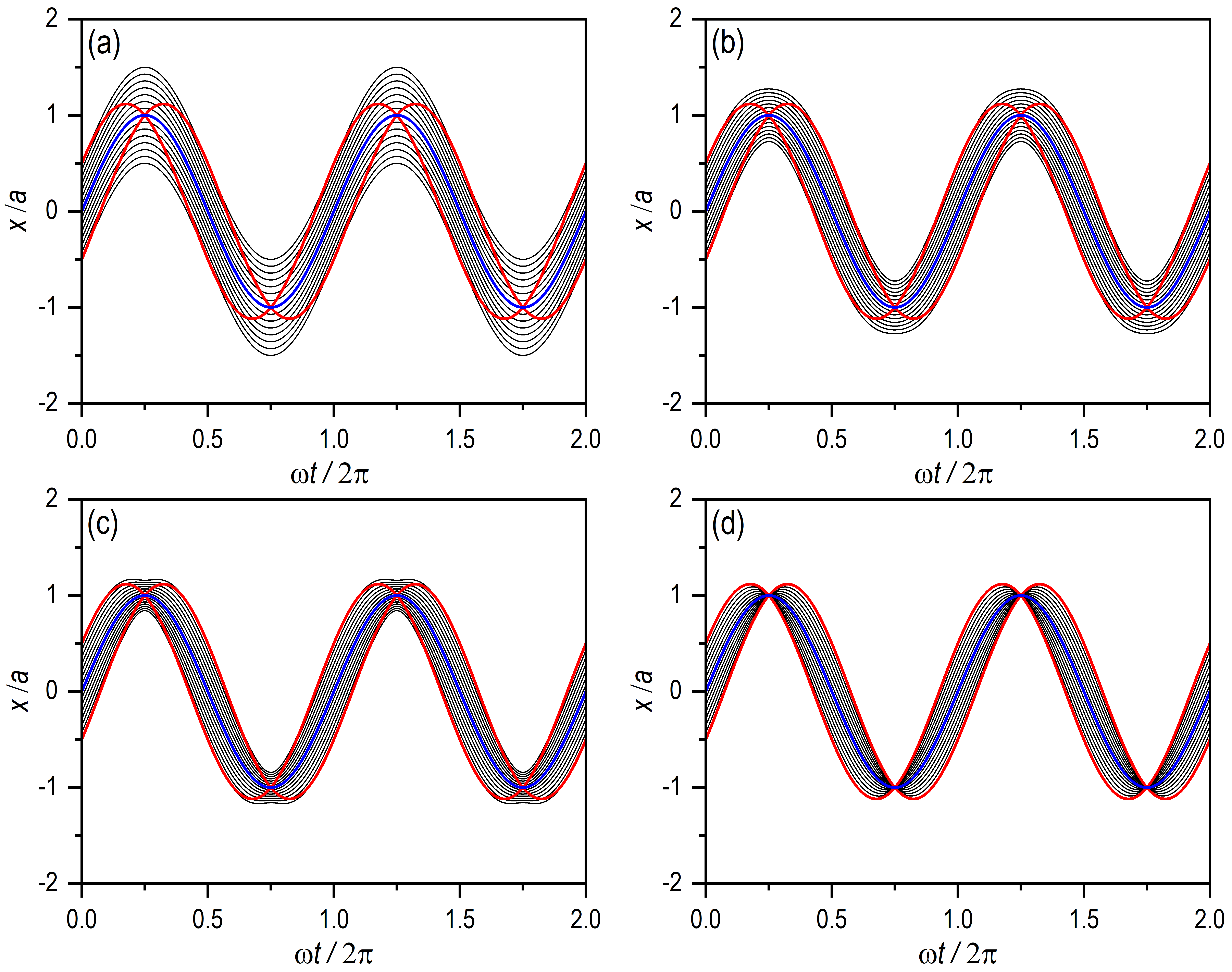
Figure 2: Gradual approach to a classical-like behavior, in a Newtonian sense, for a coherent wave packet in a harmonic oscillator with $\omega=1$ and launched from the center of the potential, at $x_{0}=0$, with $p_{0}=1$, as the coupling constant increases: (a) $\lambda=0$, (b) $\lambda=0.7$, (c) $\lambda=0.9$, and (d) $\lambda=0.999$. A set of 15 Bohmian trajectories has been used to illustrate the process, noticing that, as $\lambda$ becomes close to the unity, there is a kink denoting the position where the corresponding classical trajectories merge. Three classical trajectories superimposed to the set of Bohmian trajectories to show the turning points. The initial conditions for these trajectories are such that the blue trajectory has been launched from the center of the wave packet, while the two red ones start with the same initial conditions of their Bohmian counterparts at the margins. In all simulations here, we have considered $\hbar=1$ and $m=1$.

For simplicity in our analysis, we are going to consider Glauber states to remove any additional misleading element in the dynamics (e.g., “breathing”). Note that, since these states are regarded as the most classical ones, their associated trajectories constitute a very valuable tool to probe their dynamics, and hence to detect any particularity in the trend towards the classical limit. Thus, proceeding as in the previous section, after integrate Eq. (23) for $\lambda=1$, we obtain

$$\alpha^{r}_{t}=\frac{m\omega}{2}\frac{(2\alpha^{r}_{0}/m\omega)-\tan\omega t}{1+(2\alpha^{r}_{0}/m\omega)\tan\omega t},$$ (65)

which is totally uncoupled from the imaginary part of $\alpha_{t}$. If $\alpha^{r}_{t}$ is now substituted into Eq. (27) and then we integrate in time, we readily obtain

$$x(t)=x_{t}+\ln\left(\cos\omega t+\frac{2\alpha^{r}_{0}}{m\omega}\ \sin\omega t\right)\left[x(0)-x_{0}\right].$$ (66)

In the case of the coherent state, where $\alpha_{t}=im\omega/2$ ($\alpha^{r}_{0}=0$), this solution simplifies to

$$x(t)=x_{t}+|\cos\omega t|\left[x(0)-x_{0}\right].$$ (67)

which resembles the classical solution, except for the fact that Bohmian trajectories are kept either on one side or the other of the central one, described by the classical trajectory $x_{t}$. That is, they are prevented from coming together on the same point in the strict limit $\lambda=1$, where such a point refers to the spatial loci where a homologous set of classical trajectories focus on during the course of a full oscillation.

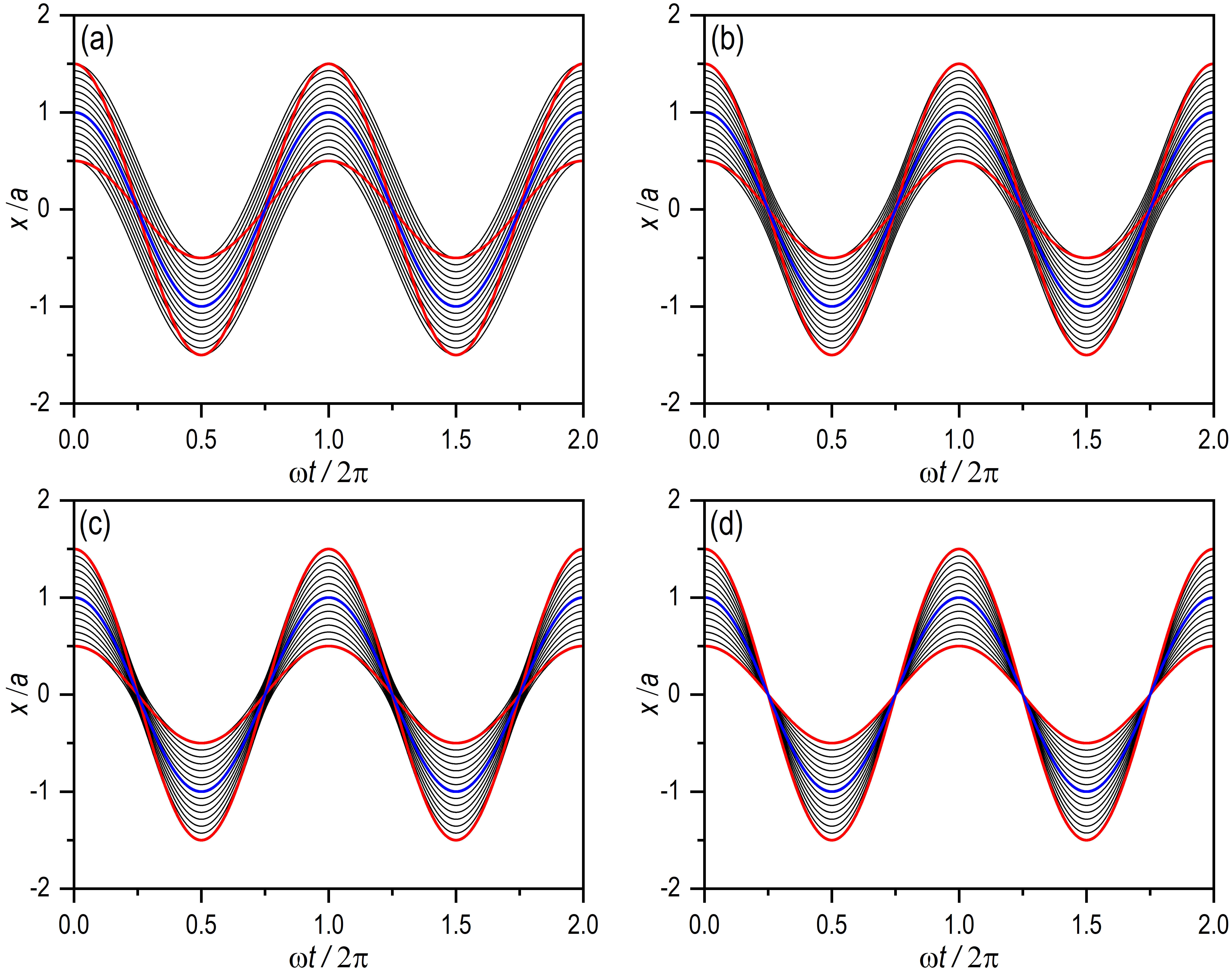
Figure 3: Gradual approach to a classical-like behavior, in a Newtonian sense, for a coherent wave packet in a harmonic oscillator with $\omega=1$ and launched from the turning point $x_{0}=1$, with $p_{0}=0$, as the coupling constant increases: (a) $\lambda=0$, (b) $\lambda=0.7$, (c) $\lambda=0.9$, and (d) $\lambda=0.999$. A set of 15 Bohmian trajectories has been used to illustrate the process, noticing that, as $\lambda$ becomes close to the unity, there is a kink denoting the position where the corresponding classical trajectories merge. Three classical trajectories superimposed to the set of Bohmian trajectories to show the turning points. The initial conditions for these trajectories are such that the blue trajectory has been launched from the center of the wave packet, while the two red ones start with the same initial conditions of their Bohmian counterparts at the margins. In all simulations here, we have considered $\hbar=1$ and $m=1$.

To illustrate the transition towards the classical limit, in Figs. 2 and 3 we have plotted sets of trajectories associated with wave packets launched from $x_{0}=0$ with $p_{0}=\sqrt{2mE}$, and from $x_{0}=x_{+}=\sqrt{2E/m\omega^{2}}$ and $p_{0}=0$, respectively. In both cases, in order to make more apparent the loci where classical trajectories focus, we have included classical trajectories launched from the center of the initial wave packet (dentoted with blue solid line) and also the same initial conditions as the two Bohmian trajectories launched from the margins (denoted with red solid line). Also, for an easier comparison, in both cases we have used the same four values for the strength coupling constant: (a) $\lambda=0$, (b) $\lambda=0.7$, (c) $\lambda=0.9$, and (d) $\lambda=0.999$. In Fig. 2, we observe a gradual transition from the characteristic parallel motion displayed by Bohmian trajectories in a fully linear regime ($\lambda=0$) to the incipient appearance of focal points in the turning points, $x_{\pm}$, which are the spatial loci where the classical trajectories with the same initial conditions meet together. Indeed, in the limit $\lambda\to 1$, in Fig. 2(d), the Bohmian and the classical trajectories are seemingly the same. The same behavior is observed in Fig. 3, although the focal point now appear at the center of the potential function, $x=0$, as it is clearly shown by the crossing undergone by the classical trajectories at that point. As it is clearly seen, the set of Bohmian trajectories gradually focuses on those points as $\lambda$ increases, until it is difficult to distinguish any difference between Bohmian and classical trajectories started at the same initial position.

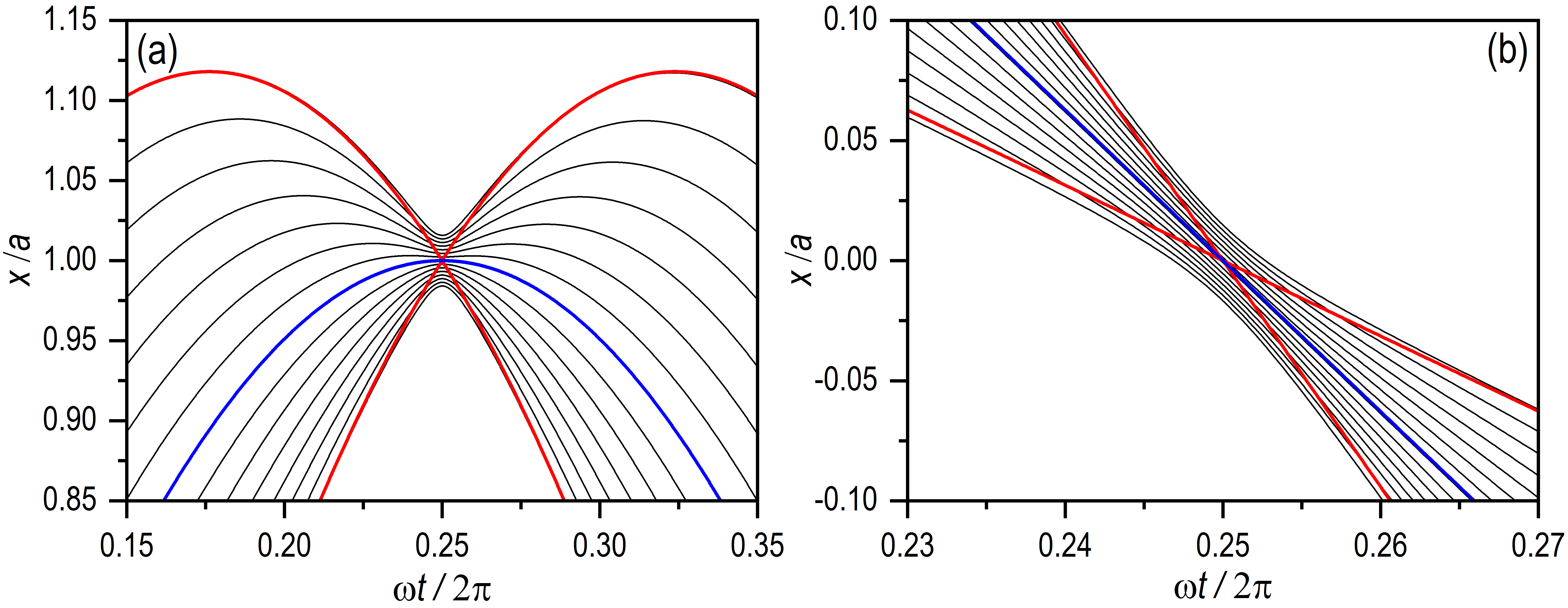
Figure 4: To better appreciate the focusing region in Figs. 2 and 3, here an enlargement of these figures is shown in panels (a) and (b), respectively, around the respective first focal points, at $\omega t=0.25$, for $\lambda=0.999$. As in the previous figures, regarding the classical trajectories at display, the blue one has been launched from the center of the wave packet, while the two red trajectories start with the same initial conditions of their Bohmian counterparts at the margins. In all simulations here, we have considered $\hbar=1$ and $m=1$.

A closer look at the foci in both cases shows, as it is seen in Fig. 4, that the approach is fast but leaving the Bohmian trajectories on one side or the other with respect to the central one (blue solid lines), unlike the behavior displayed by the classical trajectories (red solid lines), which cross at the foci. Although the simulations have been carried for $\lambda=0.999$, the trend is the same as we approach more and more the limit $\lambda\to 1$. Therefore, this behavior disproves the fact that including an anti-quantum potential leads to the classical limit. There are important differences, as we have seen in the case of the Glauber state, which is regarded as the most classical quantum state.

4 Two wave-packet interference dynamics

4.1 Free-space propagation

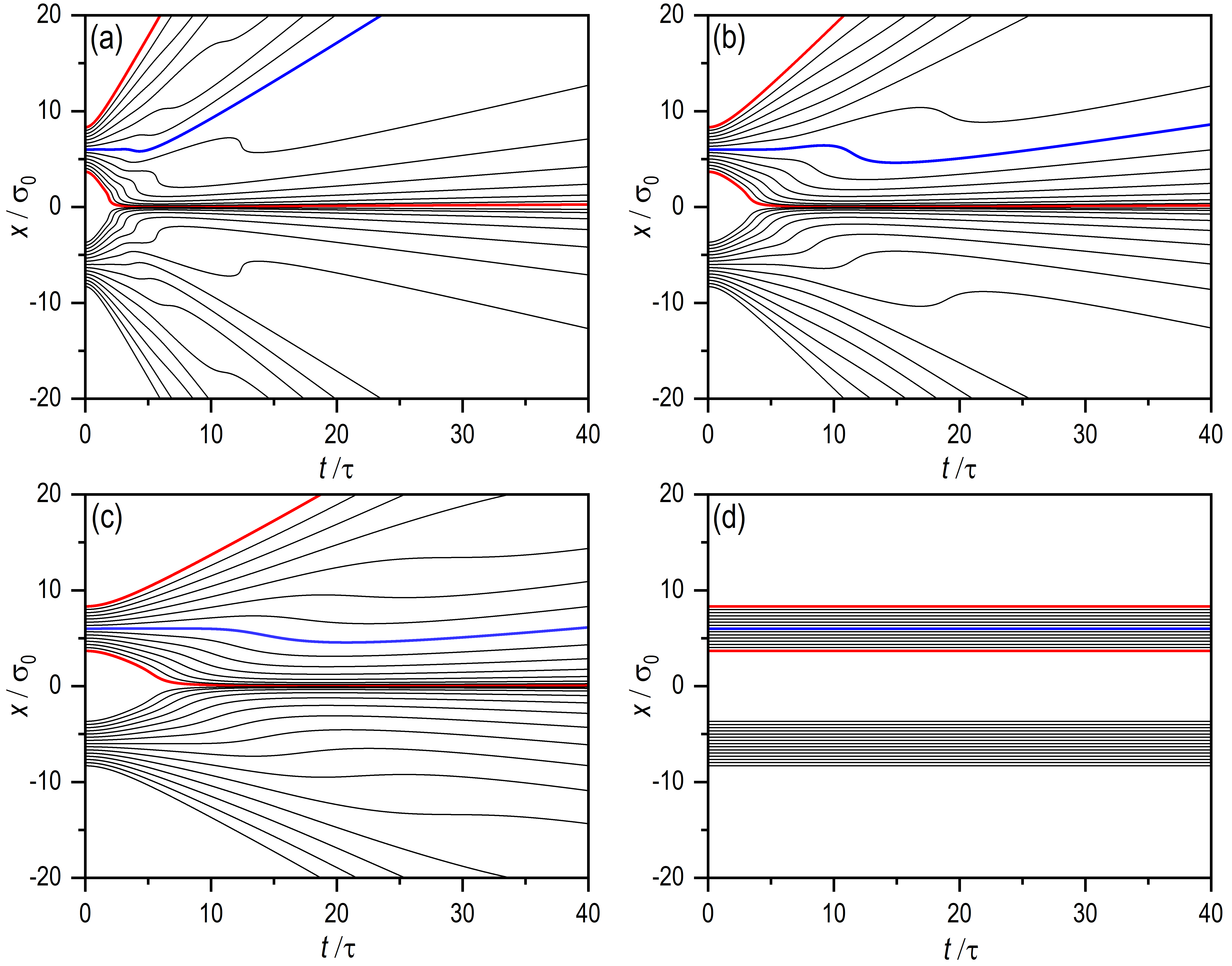
Figure 5: Suppression of the dispersion of two Gaussian wave packets in a coherent superposition, both with an initial width $\sigma_{0}=0.5$ and centered at $x_{\pm}=\pm x_{0}$ ($x_{0}=3$), as the coupling constant increases: (a) $\lambda=0$, (b) $\lambda=0.7$, (c) $\lambda=0.9$, and (d) $\lambda=1$. A set of 15 Bohmian trajectories has been launched from region covered by each wave packet in order to illustrate the process and, in turn, to show how these trajectories eventually show a classical-like behavior, in the Newtonian sense, for $\lambda=1$, as seen in panel (d). As it can be noticed, the lack of dispersion also produces that the wave packet cannot overlap and hence the trajectories will not accumulate along the directions expected from a typical interference process. The initial conditions for these trajectories are such that the blue trajectory has been launched from the center of the wave packet starting on the positive part of the $x$-axis, while the two red ones start at a $2.5\sigma_{0}$-distance from the previous one on either side. In all simulations here, we have considered $\hbar=1$, $m=1$, and $p_{0}=0$.

Apart from using the harmonic oscillator to investigate the classical limit, as seen in Sec. 3.2, one still may wonder whether there are other typical quantum traits that cannot be fully suppressed by this anti-quantum potential, such as interference. To investigate this scenario, let us remember that, in free space, we can have two interference situations worth discussing separately, namely, Young-type interference or interference produced by a head-on collision of two wave packets [31]. In both cases, we start with a superposition of two identical wave packets, like (51), localized at two different positions and with different momenta,

$$\psi(x,t) = \sqrt{N}\left(\frac{1}{2\pi\sigma_{0}^{2}}\right)^{1/4}\Bigg{[}e^{-(x-x_{1,t})^{2}/4\sigma_{0}^{2}+ip_{1,0}(x-x_{1,t})-iE_{1}t/\hbar}$$ (68)

$$\qquad\qquad+e^{-(x-x_{2,t})^{2}/4\sigma_{0}^{2}+ip_{2,0}(x-x_{2,t})-iE_{2}t/\hbar}\Bigg{]}.$$

Here, $N$ is the normalization factor of the superposition; if the center-to-center distance between the wave packets is such that $|x_{1,0}-x_{2,0}|\gg\sigma_{0}$, then $N\approx 1/\sqrt{2}$. To simplify, we consider $x_{1,0}=-x_{2,0}=x_{0}$ and $p_{1,0}=-p_{2,0}=-p_{0}$.

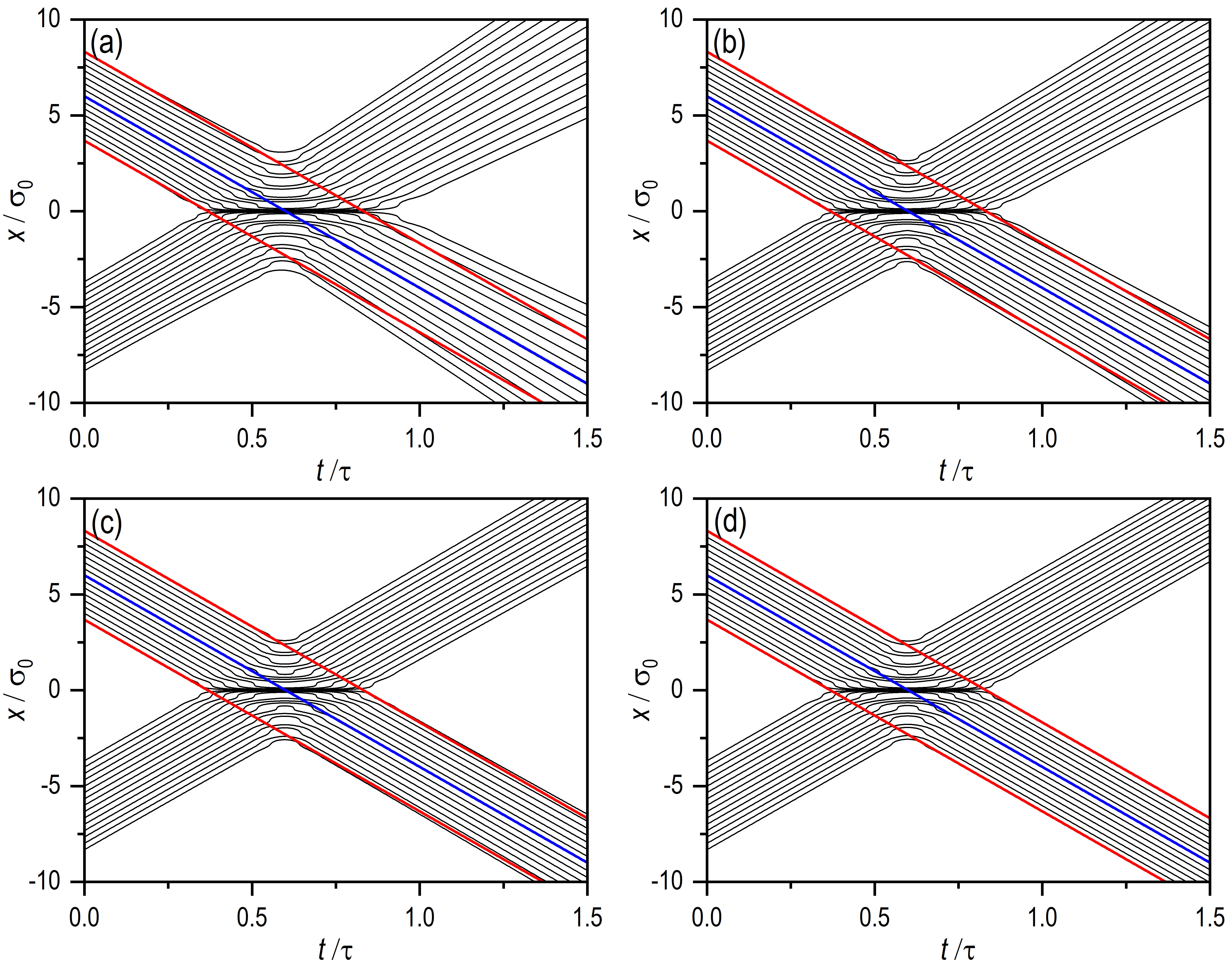
Figure 6: Same as Fig. 3, but adding an extra transverse momentum to each wave packet ($p_{\pm}=\mp 10$), so that they fully overlap at $t=3$. In this case, we find that the Bohmian trajectories do not cross the center of symmetry of the figure, although true classical trajectories would be able to do it, as it is inferred from the behavior displayed by the three classical trajectories included in the graphs. The initial conditions for these trajectories are such that the blue trajectory has been launched from the center of the wave packet starting on the positive part of the $x$-axis, while the two red ones start at a $2.5\sigma_{0}$-distance from the previous one on either side. In all simulations here, we have considered $\hbar=1$ and $m=1$.

As it is explained and discussed with detail in [31], a Young-type situation arises if $p_{0}=0$, because the gradual spreading of the wave packets eventually provokes their spatial overlapping and, hence, the appearance of interference fringes. Thus, in the long time limit, the interference profile displays a stationary shape, where the distance between consecutive minima (or maxima) increases linearly with time [37]. From a trajectory point of view, this phenomenon consists of two distinctive stages. In a first stage, the trajectories associated with each partial wave behave, in a good approximation, in an independent manner, showing the typical hyperbolic dispersion already seen in Sec. 3.1 for a free Gaussian wave packet. Once the two waves start overlapping importantly, this behavior is severely distorted, transitioning towards the second stage, where all the trajectories, as a single ensemble, start redistributing in space along different channels, each one directly related to an interference maximum. This is the behavior observed in Fig. 5(a), where we have put with different color several trajectories launched from one of the initial wave packets (with blue the one launched from the center, and with red those launched from the margins). As $\lambda$ increases, because the dispersion of the two initial wave packets is inhibited, the appearance of the channel sets of trajectories undergoes a longer and longer delay. In the limit $\lambda=1$, in Fig. 5(d), because the dispersion of the two wave packets is totally inhibited, we simply observe two separated sets of parallel trajectories.

Again, similarly to the case of a single Gaussian, if we only examine the Young-type scenario, one could conclude that all signatures of quantumness have been removed. However, if we consider the head-on collision of two wave packets, characterized by two wave packets that do not almost increase their width during the course of the propagation, but that show interference when they meet at an intermediate position, the situation is very different. This scenario is illustrated in Fig. 6. As $\lambda$ increases, we notice that, effectively, the dispersion of the wave packets is inhibited; in the limit $\lambda=1$, indeed, the Bohmian trajectories coincide with the classical ones at the margins (red solid lines). However, in analogy to the behaviors already observed with the harmonic oscillator, the divergence from a true classical behavior immediately arises if we observe what happens in the crossing region, which here is much larger than in the case of the oscillator. First, as $\lambda$ increases, interference features within this region do not disappear at all, but persist even for $\lambda=1$. Second, while the classical trajectories get across this interference region, the homologous pairs of Bohmian trajectories undergo a deflection backwards, such that the output part of a classical trajectory overlaps with the output part of a Bohmian trajectory corresponding to the opposite wave packet. Therefore, here we find another important behavior, which revels that the presence of the anti-quantum potential does not prevents the observation of typically quantum features (in this case, interference and non-crossing).

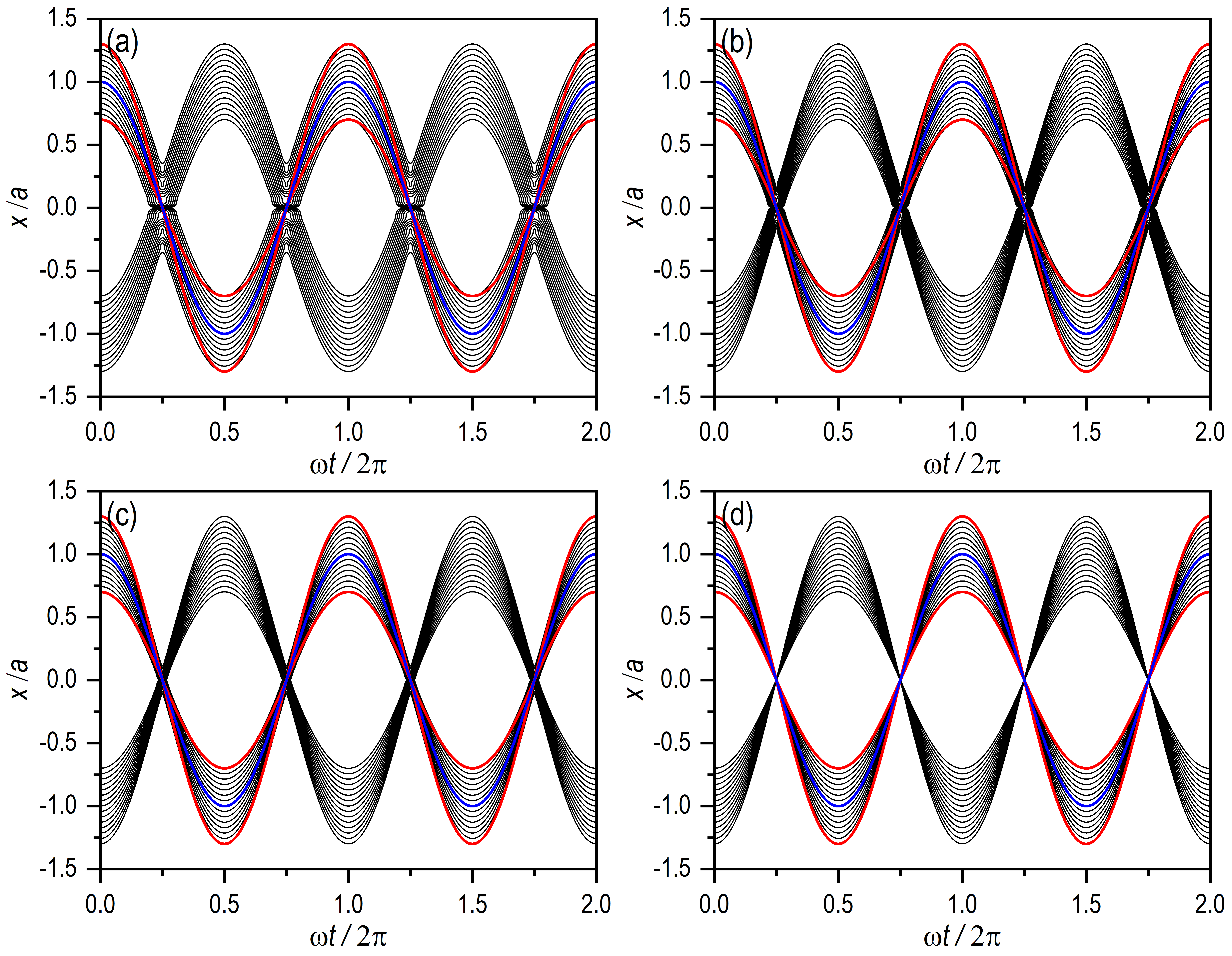
Figure 7: Same as Fig. 3, but for two wave packets inside the harmonic oscillator, each starting on an opposite turning point at $x_{\pm}=\pm x_{0}$ ($x_{0}=5$): (a) $\lambda=0$, (b) $\lambda=0.7$, (c) $\lambda=0.9$, and (d) $\lambda=0.999$. In this case, we find that the Bohmian trajectories do not cross the center of symmetry of the figure as $\lambda$ increases, although true classical trajectories would be able to do it, as the three classical trajectories superimposed make apparent. The initial conditions for these trajectories are such that the blue trajectory has been launched from the center of the wave packet, while the two red ones start with the same initial conditions of their Bohmian counterparts at the margins. In all simulations here, we have considered $\hbar=1$ and $m=1$.

4.2 Harmonic oscillator

Last, we consider another interference process, but this time inside a harmonic well, with two counter-propagating wave packets launched from opposite turning points, $x_{\pm}$. The superposition state is as described by (68), substituting the free-propagating Gaussian wave packets, but the wave packets for a harmonic oscillator (62). The results for these superpositions are represented in Fig. 7, where we have considered again four different values for the coupling strength constant: (a) $\lambda=0$, (b) $\lambda=0.7$, (c) $\lambda=0.9$, and (d) $\lambda=0.999$. In Fig. 7(a), we observe the appearance of a series of voids at the region where the two wave packets overlap. These voids arise as a consequence of the presence of nodes in the wave function, where the phase is undefined and hence also the velocity field, thus preventing the trajectories from crossing these regions and making them to undergo sudden turns, as we can also see in Fig. 6(a). Now, because Bohmian trajectories cannot cross, they undergo a bounce backwards, reaching again their initial positions in half a cycle, unlike the corresponding classical trajectories (denoted with blue and red solid lines), which require a full cycle. As $\lambda$ increases, though, the Bohmian trajectories seem to mimic the behavior observed in the classical trajectories, as it is seen in Fig. 7(d), with the ensembles coming from each wave packet focusing at the center of the potential function.

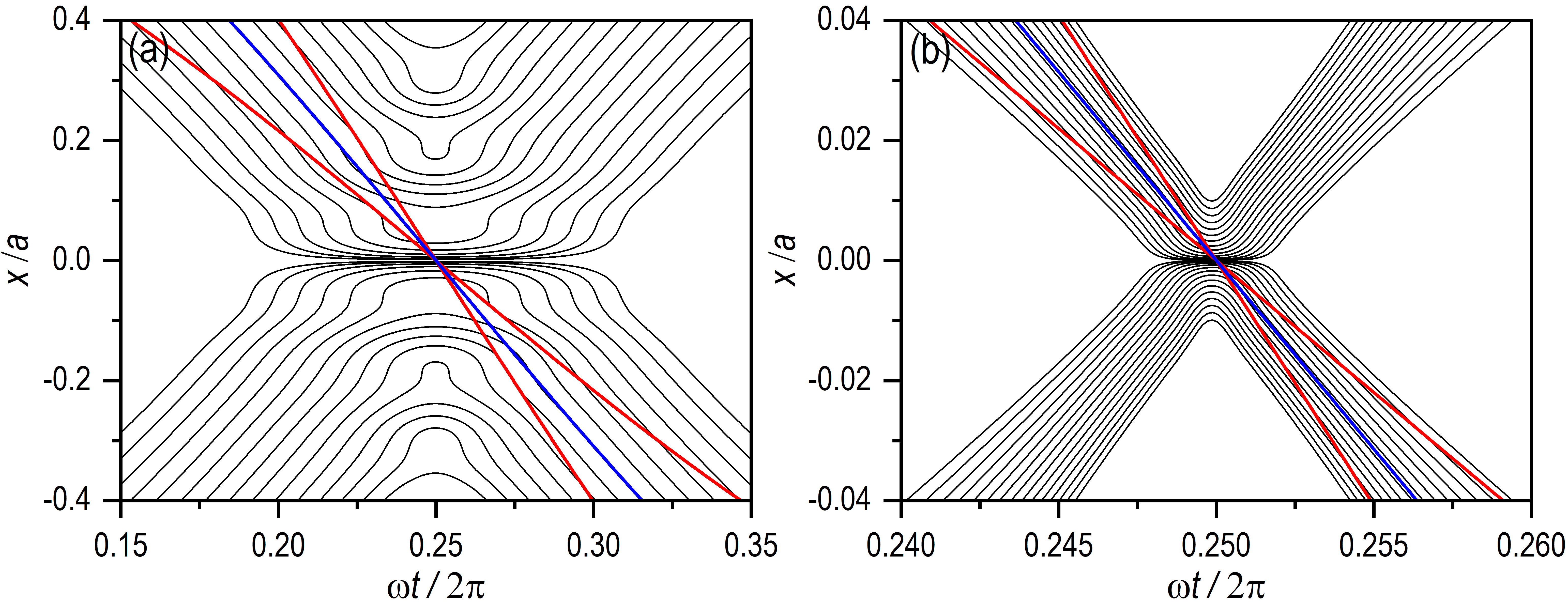
Figure 8: To better appreciate the details of the region where the two sets of Bohmian trajectories undergo the bounce backwards in Figs. 7a ($\lambda=0$) and 7d ($\lambda=0.999$), panels (a) and (b) show here, respectively, an enlargement around of the corresponding regions. The maximum approach takes place at $\omega t=0.25$. As in Fig. 7, the initial conditions for the trajectories plotted are such that the blue trajectory has been launched from the center of the wave packet, while the two red ones start with the same initial conditions of their Bohmian counterparts at the margins. In all simulations here, we have considered $\hbar=1$ and $m=1$.

To better understand what happens at the focus, in Fig. 8 we show an enlargement in a neighboring region around it for the cases displayed in Figs. 7(a) and 7(b), where we can clearly observe the presence of voids in the first case, and the focusing effect in the second one. Two remarks are worth noting. First, note the order of magnitude of difference between the two regions displayed despite in both cases we have used exactly the same initial conditions, which gives an idea of the induced focusing. Should we have used a $\lambda$-value closer to 1, the dimensions of the focus region would have decreased even more. Second, although we do not observe the presence of nodes in Fig. 8(b), this does not mean that they do not form. In symmetric head-on collisions (i.e., whenever both wave packets have exactly the same properties and they propagate with the same speed in opposite directions), the nodes formed when both wave packets fully overlap are separated by a distance $\Delta x=\pi\hbar/p_{0}$ provided the dispersion at that time with respect is negligible compared to the initial dispersion. In all panels in Fig. 6, this is precisely the case, so all the nodes are separated a distance $\Delta x\approx 0.31$ (their positions can be inferred from the sudden turns undergone by the trajectories at $t=0.3$). In the case of the two wave packet inside the harmonic well, the distance between nodes is given by the expression $\Delta x=\pi\hbar/m\omega x_{0}\approx\approx 0.63$, as it can be clearly seen in Fig. 8(a). As the focusing becomes stronger for sets of trajectories with the same initial conditions, it is clear that they will pack closer and closer, in distances of orders much below $\Delta x$, and hence we will not be able to see them, which is the case of Fig. 8(b). To do so, and hence to obtain a representation analogous to that of Fig. 6(d), we would therefore need to consider a much wider range for initial conditions around the center of each wave packet. Of course, this would imply considering to cover with initial conditions regions far away from the centroids of the wave packets, where the probability density already is already negligible (note that in all cases here we have chosen initial conditions reaching regions with very low values of the probability density).

5 Final remarks

Here we have analyzed the consequences of introducing nonlinearities in the Schrödinger equation in the form of the so-called Bohm’s quantum potential. In the literature, this has been widely regarded as a means to recover the classical limit, since, following the usual Bohmian prescription [24], the addition of this anti-quantum potential gives rise to an equation of motion for the phase field identical to the classical Hamilton-Jacobi equation. Hence, if from this latter equation one obtains the trajectories of classical mechanics, from the phase of the classical wave function resulting from the corresponding nonlinear Schrödinger equation one should also obtain Bohmian trajectories that behave like classical trajectories. Now, this hypothesis omits the fact that, while in classical mechanics it is allowed a bi-valuation of the momentum (also given by the gradient of the classical action), the Schrödinger equation is constructed under the implicit assumption that their solutions are single-valued, except for a constant global phase factor. This means that the phase of the wave function is also single valued, except for that constant factor, but the velocity field has to be single-valued. The most striking consequence from this constraint is the well-known Bohmian non-crossing rule. Nonetheless, within a more general perspective, this is nothing but a direct physical consequence arising from the preservation of the phase coherence, present in any wave theories, regardless of the physical system described and, in particular, of whether the corresponding equation is linear or nonlinear.

To analyze the above mentioned consequences led by the anti-quantum potential, we have considered the propagation of Gaussian wave packets both in free space and inside of a harmonic potential, as well as the corresponding superpositions. Given that Gaussian wave packets are exact solutions of the Schrödinger equation for potential functions that are polynomials of up to second order, and that the addition of the anti-quantum potential is analogous to partly considering a kinetic-type contribution, we have obtained exact solutions in all cases for both the linear and the fully nonlinear cases. For any other intermediate case, we have obtained analytical equations of motion for the parameters describing the evolution of the Gaussian as well as for the corresponding trajectories. Numerically integrating the latter, we have investigated the behavior for various values of the coupling strength constant, from $\lambda=0$ to $\lambda=1$.

From the results obtained, we conclude that the presence of the anti-quantum potential, although provides us with behaviors analogous to those displayed by classical trajectories, it is also revealed that its only presence does not prevent the observation of typically quantum features directly connected with the preservation of the quantum coherence, such as interference and non-crossing. This situation is similar to that found when dealing with trajectories that describe fully incoherent quantum systems, but that are obtained from the associated reduced density matrix [38]. In these situations, groups of trajectories associated with two different wave packets do not cross the symmetry axis between them, because the phase coherence connected to the information about having the two wave packets involved at the same time in the system dynamics is still preserved (even though any interference trait is fully washed out). Obtaining a genuine classical behavior thus requires a suppression of the wave packet that the trajectories are not associated with [39], which is the case when an environment is present [37].

References

- [1] W. H. Zurek, Decoherence and the transition from quantum to classical – revisited, Los Alamos Science 27 (2002) 86–109.
- [2] D. Giulini, E. Joos, C. Kiefer, J. Kupsch, I.-O. Stamatescu, H. D. Zeh, Decoherence and the Appearance of a Classical World in Quantum Theory, 2nd Edition, Springer, 1996, Berlin.
- [3] M. Schlosshauer, Decoherence, the measurement problem, and interpretations of quantum mechanics, Rev. Mod. Phys. 76 (2005) 1267–1305.
- [4] M. Schlosshauer, Quantum decoherence, Phys. Rep. 831 (2019) 1–57, quantum decoherence.
- [5] M. Schlosshauer, Decoherence and the Quantum-to-Classical Transition, Springer, Berlin, 2007.
- [6] H.-P. Breuer, F. Petruccione, The Theory of Open Quantum Systems, Oxford University Press, Oxford, 2002.
- [7] L. Diósi, Quantum stochastic processes as models for state vector reduction, J. Phys. A 21 (1988) 2885–2898.
- [8] N. Gisin, I. C. Percival, The quantum-state diffusion model applied to open systems, J. Phys. A 25 (1992) 5677–5691.
- [9] I. C. Percival, Quantum State Diffusion, Cambridge University Press, Cambridge, 1998.
- [10] M. D. Kostin, On the schrödinger-langevin equation, J. Chem. Phys. 57 (1972) 3589–3591.
- [11] R. Katz, P. Gossiaux, The schrödinger–langevin equation with and without thermal fluctuations, Ann. Phys. 368 (2016) 267–295.
- [12] H. Losert, F. Ullinger, M. Zimmermann, M. A. Efremov, E. M. Rasel, W. P. Schleich, The kostin equation, the deceleration of a quantum particle and coherent control, J. Low Temp. Phys. 210 (2023) 4–50.
- [13] D. Schuch, K.-M. Chung, H. Hartmann, Nonlinear schrödinger-type field equation for the description of dissipative systems. i. derivation of the nonlinear field equation and one-dimensional example, J. Math. Phys. 24 (1983) 1652–1660.
- [14] D. Schuch, K.-M. Chung, H. Hartmann, Nonlinear schrödinger-type field equation for the description of dissipative systems. ii. frictionally damped motion in a magnetic field, Int. J. Quantum Chem. 25 (1984) 391–410.
- [15] D. Schuch, K.-M. Chung, H. Hartmann, Nonlinear schrödinger-type field equation for the description of dissipative systems. iii. frictionally damped free motion as an example for an aperiodic motion, Phys. Rev. A 25 (1984) 3086–3092.
- [16] L. Diósi, Gravitation and quantum-mechanical localization of macro-objects, Physics Letters A 105 (4) (1984) 199–202.
- [17] R. Penrose, On gravity’s role in quantum state reduction, Gen. Rev. Grav. 28 (1996) 581–600.
- [18] J. H. V. Vleck, The correspondence principle in the statistical interpretation of quantum mechanics, Proc. Natl. Acad. Sci. 14 (1928) 178–188.
- [19] R. Schiller, Quasi-classical theory of the nonspinning electron, Phys. Rev. 125 (1962) 1100–1108.
- [20] N. Rosen, Identical motion in quantum and in classical mechanics, Am. J. Phys. 32 (1964) 377–379.
- [21] N. Rosen, The relation between classical and quantum mechanics, Am. J. Phys. 32 (1964) 597–600.
- [22] N. Rosen, Mixed states in classical mechanics, Am. J. Phys. 33 (1965) 146–150.
- [23] N. Rosen, Quantum particles and classical particles, Found. Phys. 16 (1986) 687–700.
- [24] P. R. Holland, The Quantum Theory of Motion, Cambridge University Press, Cambridge, 1993.
- [25] W. P. Schleich, D. M. Greenberger, D. H. Kobe, M. O. Scully, Schrödinger equation revisited, Proc. Nat. Acad. Sci. 110 (14) (2013).
- [26] C.-C. Chou, Trajectory description of the quantum–classical transition for wave packet interference, Annals of Physics 371 (2016) 437–459.
- [27] C.-C. Chou, Trajectory-based understanding of the quantum–classical transition for barrier scattering, Annals of Physics 393 (2018) 167–183.
- [28] A. Benseny, D. Tena, X. Oriols, On the classical schrödinger equation, Fluct. Noise Lett. 15 (2016) 1640011.
- [29] L. I. Schiff, Quantum Mechanics, 3rd Edition, McGraw-Hill, Singapore, 1968.
- [30] D. Bohm, A suggested interpretation of the quantum theory in terms of “hidden” variables. i, Phys. Rev. 85 (1952) 166–179.
- [31] A. S. Sanz, S. Miret-Artés, A trajectory-based understanding of quantum interference, J. Phys. A: Math. Theor. 41 (43) (2008) 435303.
- [32] D. Bohm, B. J. Hiley, The Undivided Universe, Routledge, New York, 1993.
- [33] A. S. Sanz, S. Miret-Artés, A Trajectory Description of Quantum Processes. II. Applications, Vol. 831 of Lecture Notes in Physics, Springer, Berlin, 2014.
- [34] A. S. Sanz, Bohm’s approach to quantum mechanics: Alternative theory or practical picture?, Front. Phys. 14 (2019) 11301.
- [35] A. S. Sanz, S. Miret-Artés, Quantum phase analysis with quantum trajectories: A step towards the creation of a bohmian thinking, Am. J. Phys. 80 (2012) 525–533.
- [36] E. J. Heller, Time-dependent approach to semiclassical dynamics, J. Chem. Phys. 62 (1975) 1544–1555.
- [37] A. S. Sanz, Young’s experiment with entangled bipartite systems: The role of underlying quantum velocity fields, Entropy 25 (7) (2023).
- [38] A. S. Sanz, F. Borondo, A quantum trajectory description of decoherence, Eur. Phys. J. D 44 (2007) 319–326.
- [39] A. S. Sanz, F. Borondo, Contextuality, decoherence and quantum trajectories, Chem. Phys. Lett. 478 (2009) 301–306.