Describing Differences in Image Sets with Natural Language

Abstract

How do two sets of images differ? Discerning set-level differences is crucial for understanding model behaviors and analyzing datasets, yet manually sifting through thousands of images is impractical. To aid in this discovery process, we explore the task of automatically describing the differences between two sets of images, which we term Set Difference Captioning. This task takes in image sets $\mathcal{D}_{A}$ and $\mathcal{D}_{B}$, and outputs a description that is more often true on $\mathcal{D}_{A}$ than $\mathcal{D}_{B}$. We outline a two-stage approach that first proposes candidate difference descriptions from image sets and then re-ranks the candidates by checking how well they can differentiate the two sets. We introduce VisDiff, which first captions the images and prompts a language model to propose candidate descriptions, then re-ranks these descriptions using CLIP. To evaluate VisDiff, we collect VisDiffBench, a dataset with 187 paired image sets with ground truth difference descriptions. We apply VisDiff to various domains, such as comparing datasets (e.g., ImageNet vs. ImageNetV2), comparing classification models (e.g., zero-shot CLIP vs. supervised ResNet), characterizing differences between generative models (e.g., StableDiffusionV1 and V2), and discovering what makes images memorable. Using VisDiff, we are able to find interesting and previously unknown differences in datasets and models, demonstrating its utility in revealing nuanced insights.

Figure 2: VisDiff algorithm. VisDiff consists of a GPT-4 proposer on BLIP-2 generated captions and a CLIP ranker. The proposer takes randomly sampled image captions from $\mathcal{D}_{A}$ and $\mathcal{D}_{B}$ and proposes candidate differences. The ranker takes these proposed differences and evaluates them across all the images in $\mathcal{D}_{A}$ and $\mathcal{D}_{B}$ to assess which ones are most true.

1 Introduction

What kinds of images are more likely to cause errors in one classifier versus another [11, 18]? How do visual concepts shift from a decade ago to now [33, 53, 20]? What types of images are more or less memorable for humans [17]? Answering these questions can help us audit and improve machine learning systems, understand cultural changes, and gain insights into human cognition.

Although these questions have been independently studied in prior works, they all share a common desideratum: discovering differences between two sets of images. However, discovering differences in many, potentially very large, sets of images is a daunting task for humans. For example, one could gain insights into human memory by discovering systematic differences between memorable images and forgettable ones, but finding these differences may require scanning through thousands of images. An automated solution would be more scalable.

In this work, we explore the task of describing differences between image sets, which we term Set Difference Captioning (Figure 1). Specifically, given two sets of images $\mathcal{D}_{A}$ and $\mathcal{D}_{B}$, set difference captioning aims to find the most salient differences by generating natural language descriptions that are more often true in $\mathcal{D}_{A}$ than $\mathcal{D}_{B}$. We show in Section 6 that many dataset and model analysis tasks can be formulated in terms of set difference captioning, and methods that address this problem can help humans discover new patterns in their data.

Set difference captioning presents unique challenges to current machine learning systems, since it requires reasoning over all the given images. However, no existing models in the vision and language space can effectively reason about thousands of images as input. Furthermore, while there are usually many valid differences between $\mathcal{D}_{A}$ and $\mathcal{D}_{B}$, end users are typically interested in what can most effectively differentiate between the two sets. For example, “birthday party” is a valid difference in Figure 1, but “people posing for a picture” better separates the sets.

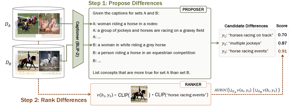
We introduce a two-stage proposer-ranker approach [49, 50, 53] for set difference captioning that addresses these challenges. As shown in Figure 2, the proposer randomly samples subsets of images from $\mathcal{D}_{A}$ and $\mathcal{D}_{B}$ to generate a set of candidate differences in natural language. The ranker then scores the salience and significance of each candidate by validating how often this difference is true for individual samples in the sets. Within the proposer-ranker framework, there are many plausible design choices for each component, and in this work we investigate three categories of proposers and rankers that utilize different combinations of models pre-trained with different objectives.

To evaluate design choices, we construct VisDiffBench (Figure 3), a dataset consisting of 187 paired image sets with ground-truth differences. We also propose a large language model-based evaluation to measure correctness. By benchmarking different designs on VisDiffBench, we identify our best algorithm, VisDiff, which combines a proposer based on BLIP-2 captions and GPT-4 with a ranker based on CLIP features. This method accurately identifies 61% and 80% of differences using top-1 and top-5 evaluation even on the most challenging split of VisDiffBench.

Finally, we apply VisDiff to a variety of applications, such as finding dataset differences, comparing model behaviors, and understanding questions in cognitive science. VisDiff identifies both differences that can be validated by prior works, as well as new findings that may motivate future investigation. For example, VisDiff uncovers ImageNetV2’s temporal shift compared to ImageNet [35, 5], CLIP’s strength in recognizing texts within images compared to ResNet [34, 13], StableDiffusionV2 generated images’ stylistic changes compared to StableDiffusionV1 [38], and what images are more memorable by humans [16]. These results indicate that the task of set difference captioning is automatic, versatile, and practically useful, opening up a wealth of new application opportunities for future work and potentially mass-producing insights unknown to even experts across a wide range of domains.

2 Related Works

Many prior works explored difference captioning [22, 21, 1, 46] and change captioning [31, 2, 19], which aim to describe differences between a single pair of images with language. Recent large visual language models (VLMs) like GPT-4V [30] have shown promise in describing differences in small groups of images. However, the question of how to scale this problem to sets containing thousands of images remains unanswered. Meanwhile, some existing works in vision tackle understanding large amounts of visual data through finding concept-level prototypes [42, 8], “averaging” large collections of images [52], using simple methods like RGB value analysis [41, 28], or using a combination of detectors and classifiers to provide dataset level statistics [44]. However, they do not describe the differences in natural language, which is flexible and easy to interpret.

Our work draws inspiration from D3 [49] and D5 [50] frameworks, which use large language models (LLMs) to describe differences between text datasets. A recent work GS-CLIP [53] applied a similar framework as D3 in the image domain, using CLIP features to retrieve differences from a pre-defined text bank. While this work targets the task of set difference captioning, it struggles at generating descriptive natural language and has a limited evaluation on the MetaShift [24] dataset that we found contains a significant amount of noise. Inspired by D3 [49], our study advances a proposer-ranker framework tailored for the visual domain, leveraging large visual foundation models and a well-designed benchmark dataset. The versatility and effectiveness of our approach are further demonstrated through applications across a variety of real-world scenarios, underscoring its potential impact and utility in practical settings.

Lastly, the set difference captioning setting is closely related to the field of explainable computer vision. Traditional explainable computer vision methodologies have predominantly concentrated on interpreting features or neurons within deep neural networks, as exemplified by approaches like LIME [37], CAM [51], SHAP [27], and MILAN [15]. Recent shifts towards a data-centric AI paradigm have sparked a wave of research focusing on identifying influential data samples that impact predictions [32, 39], and on discerning interpretable data segments [4, 11, 6], thereby elucidating model behaviors. Our set difference captioning aligns with these objectives, offering a unique, purely data-driven approach to understanding and explaining differences in image sets with natural language.

3 Set Difference Captioning

In this section, we first describe the task of set difference captioning, then introduce VisDiffBench, which we use to benchmark performance on this task.

Figure 3: Top 5 descriptions generated by the caption-based, image-based, and feature-based proposer. All the top 5 descriptions from the caption-based proposer and the top 2 from the image-based proposer identify the ground-truth difference between “practicing yoga” and “meditating”, while feature-based fails. We report AUROC scores from the same feature-based ranker described in Section 4.2.

3.1 Task Definition

Given two image datasets $\mathcal{D}_{A}$ and $\mathcal{D}_{B}$, the goal of set difference captioning (SDC) is to generate a natural language description $y$ that is more true in $\mathcal{D}_{A}$ compared to $\mathcal{D}_{B}$. For example, in Figure 3, both $\mathcal{D}_{A}$ and $\mathcal{D}_{B}$ contain images of horses, but the images from $\mathcal{D}_{A}$ are all from racing events, so a valid choice of $y$ would be “horse racing events”.

In our benchmarks below, we annotate ($\mathcal{D}_{A}$, $\mathcal{D}_{B}$) with a ground truth $y^{*}$ based on knowledge of the data-generating process. In these cases, we consider an output $y$ to be correct if it matches $y^{*}$ up to semantic equivalence (see Section 3.3 for details). In our applications (Section 6), we also consider cases where the ground truth $y^{*}$ is not known.

3.2 Benchmark

To evaluate systems for set difference captioning, we construct VisDiffBench, a benchmark of 187 paired image sets each with a ground-truth difference description. To create VisDiffBench, we curated a dataset PairedImageSets that covers 150 diverse real-world differences spanning three difficulty levels. We supplemented this with 37 differences obtained from two existing distribution shift benchmarks, ImageNet-R and ImageNet^∗. Aggregate statistics for VisDiffBench are given in Table 1.

Dataset	# Paired Sets	# Images Per Set
ImageNetR (sampled)	14	500
ImageNet∗ (sampled)	23	500
PairedImageSets-Easy	50	100
PairedImageSets-Medium	50	100
PairedImageSets-Hard	50	100

Table 1: Summary of VisDiffBench. In experiments, we merge ImageNetR and ImageNet^∗ because they have limited sets.

ImageNet-R: ImageNet-R [14] contains renditions of 200 ImageNet classes across 14 categories (e.g., art, cartoon, painting, sculpture, sketch). For each category, we set $y^{*}$ to be the name of the category, $\mathcal{D}_{A}$ to be 500 images sampled from that category, and $\mathcal{D}_{B}$ to be 500 original ImageNet images sampled from the same 200 classes.

ImageNet^∗: ImageNet^∗ [43] contains 23 categories of synthetic images transformed from original ImageNet images using textual inversion. These categories include particular style, co-occurrence, weather, time of day, etc. For instance, one category, “at dusk,” converts ImageNet images with the prompt “a photo of a [inverse image token] at dusk”. We generated differences analogously to ImageNet-R, taking $\mathcal{D}_{A}$ to be 500 image samples from the category and $\mathcal{D}_{B}$ to be 500 original ImageNet images.

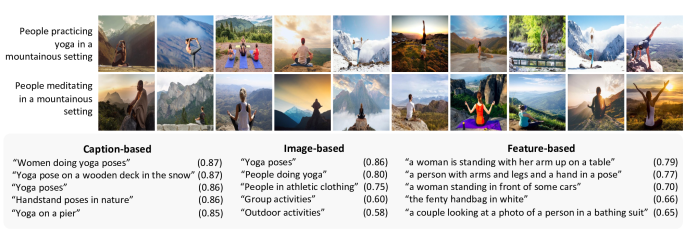
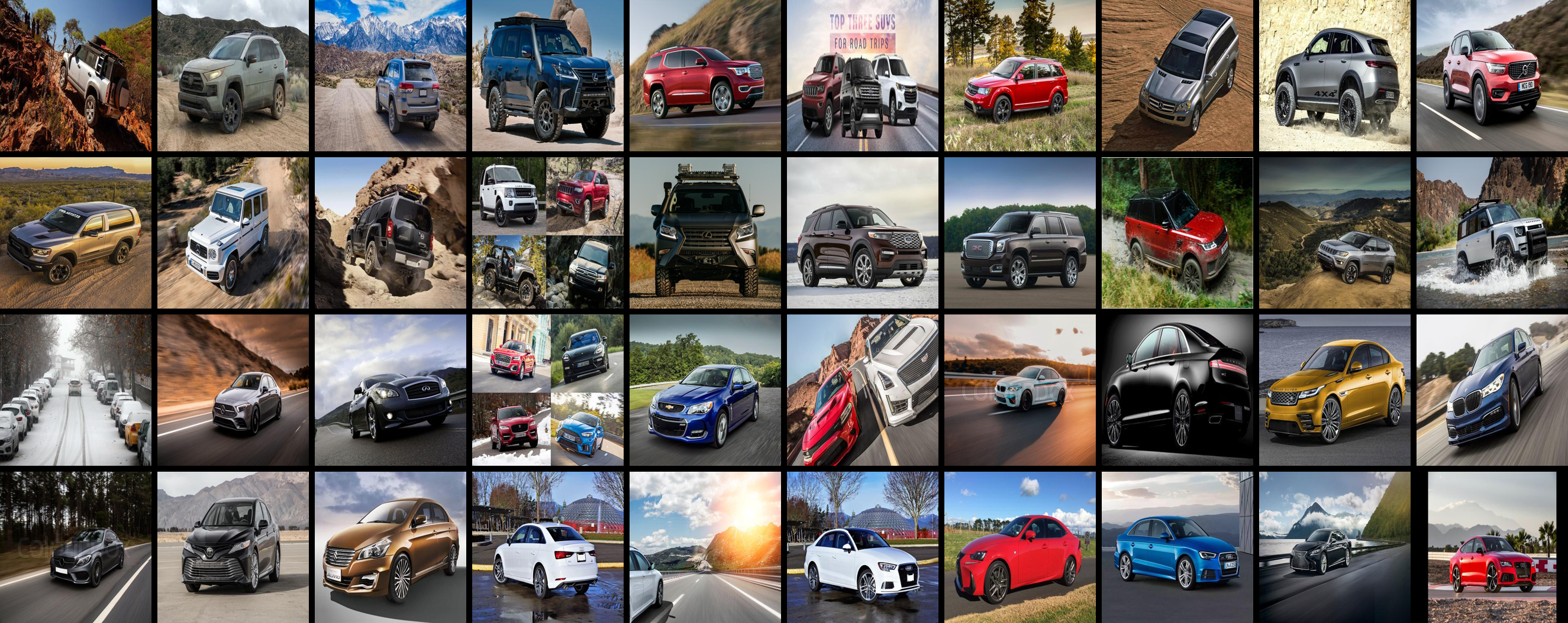
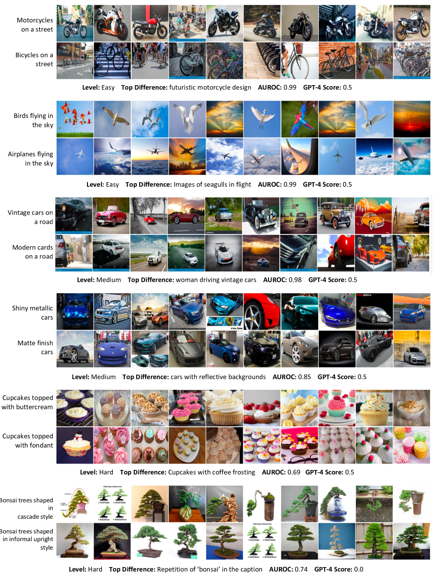
PairedImageSets: ImageNetR and ImageNet^∗ mainly capture stylistic differences, and only contain 37 differences in total. To address these shortcomings, we construct PairedImageSets, consisting of 150 paired image sets representing diverse differences. The dataset was built by first prompting GPT-4 to generate 150 paired sentences with three difficulty levels of differences (see Appendix A for exact prompts). Easy level represents apparent difference (e.g., “dogs playing in a park” vs. “cats playing in a park”), medium level represents fine-grained difference (e.g., “SUVs on the road” vs. “sedans on the road”), and hard level represents subtle difference (e.g., “people practicing yoga in a mountainous setting” vs. “people meditating in a mountainous setting”).

Once GPT-4 generates the 150 paired sentences, we manually adjusted the annotated difficulty levels to match the criteria above. We then retrieved the top 100 images from Bing for each sentence. As a result, we collected 50 easy, 50 medium, and 50 hard paired image sets, with 100 images for each set. One example pair from this dataset is shown in Figure 3, with further examples and a complete list of paired sentences provided in Appendix A. We will release this dataset and the data collection pipeline.

3.3 Evaluation

To evaluate performance on VisDiffBench, we ask algorithms to output a description $y$ for each ($\mathcal{D}_{A}$, $\mathcal{D}_{B}$) pair and compare it to the ground truth $y^{*}$. To automatically compute whether the proposed difference is semantically similar to the ground truth, we prompt GPT-4 to categorize similarity into three levels: 0 (no match), 0.5 (partially match), and 1 (perfect match); see Appendix A for the exact prompt.

To validate this metric, we sampled 200 proposed differences on PairedImageSets and computed the correlation of GPT-4’s scores with the average score across four independent annotators. We observe a high Pearson correlation of 0.80, consistent with prior findings that large language models can align well with human evaluations [48, 9].

We will evaluate systems that output ranked lists of proposals for each ($\mathcal{D}_{A}$, $\mathcal{D}_{B}$) pair. For these systems, we measure Acc@k, which is the highest score of any of the top-k proposals, averaged across all 187 paired image sets.

Proposer	Ranker	PIS-Easy		PIS-Medium		PIS-Hard		ImageNet-R/*
		Acc@1	Acc@5	Acc@1	Acc@5	Acc@1	Acc@5	Acc@1	Acc@5
LLaVA-1.5 Image	CLIP Feature	0.71	0.81	0.39	0.49	0.28	0.43	0.27	0.39
BLIP-2 Feature	CLIP Feature	0.48	0.69	0.13	0.33	0.12	0.23	0.68	0.85
GPT-4 Caption	Vicuna-1.5 Caption	0.60	0.92	0.49	0.77	0.31	0.61	0.42	0.70
GPT-4 Caption	LLaVA-1.5 Image	0.78	0.99	0.58	0.80	0.38	0.62	0.78	0.88
GPT-4 Caption	CLIP Feature	0.88	0.99	0.75	0.86	0.61	0.80	0.78	0.96

Table 2: Results on VisDiffBench. GPT-4 caption-based proposer and CLIP feature-based ranker consistently outperform other proposers and rankers by a large margin. We use this combination as the final VisDiff algorithm. PIS is short for PairedImageSets.

4 Our Method: VisDiff

It is challenging to train a neural network to directly predict $y$ based on $\mathcal{D}_{A}$ and $\mathcal{D}_{B}$: $\mathcal{D}_{A}$ and $\mathcal{D}_{B}$ can be very large in practice, while currently no model can encode large sets of images and reliably reason over them. Therefore, we employ a two-stage framework for set difference captioning, using a proposer and a ranker [49, 50]. The proposer takes random subsets $\mathcal{S}_{A}\subseteq\mathcal{D}_{A}$ and $\mathcal{S}_{B}\subseteq\mathcal{D}_{B}$ and proposes differences. The ranker takes these proposed differences and evaluates them across all of $\mathcal{D}_{A}$ and $\mathcal{D}_{B}$ to assess which ones are most true. We explore different choices of the proposer and ranker in the next two subsections. Full experiment details for this section, including the prompts for the models, can be found in Appendix B.

4.1 Proposer

The proposer takes two subsets of images $\mathcal{S}_{A}$ and $\mathcal{S}_{B}$ as inputs and outputs a list $\mathcal{Y}$ of natural language descriptions that are (ideally) more true on $\mathcal{S}_{A}$ than $\mathcal{S}_{B}$. We leverage visual language models (VLM) as the proposer in three different ways: from the images directly, from the embeddings of the images, or by first captioning images and then using a language model. In all cases, we set $|\mathcal{S}_{A}|=|\mathcal{S}_{B}|=20$ based on ablations.

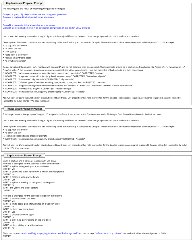
Image-based Proposer: We arrange the 20+20 input images into a single 4-row, 10-column grid and feed this as a single image into a VLM (in our case, LLaVA-1.5 [25]). We then prompt the VLM to propose differences between the top and bottom half of images.

Feature-based Proposer: We embed images from $\mathcal{S}_{A}$ and $\mathcal{S}_{B}$ into the VLM’s visual representation space, then subtract the mean embeddings of $\mathcal{S}_{A}$ and $\mathcal{S}_{B}$. This subtracted embedding is fed into VLM’s language model to generate a natural language description of the difference. We use BLIP-2 [23] for this proposer.

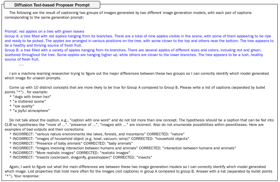
Caption-based Proposer: We first use the VLM to generate captions of each image in $\mathcal{S}_{A}$ and $\mathcal{S}_{B}$. Then, we prompt a pure language model to generate proposed differences between the two sets of captions. We use BLIP-2 to generate the captions and GPT-4 to propose differences.

Experiments in Section 5.1 show that the caption-based proposer works best, so we will take it as our main method and the other two as baselines. To further improve performance, we run the proposer multiple times over different sampled sets $\mathcal{S}_{A}$ and $\mathcal{S}_{B}$, then take the union of the proposed differences as inputs to the ranker.

4.2 Ranker

Since the proposer operates on small subsets $\mathcal{S}_{A}$ and $\mathcal{S}_{B}$ and could generate invalid or noisy differences, we employ a ranker to validate and rank the proposed differences $y\in\mathcal{Y}$. The ranker sorts hypotheses by computing a difference score $s_{y}=\mathbb{E}_{x\in\mathcal{D}_{A}}v(x,y)-\mathbb{E}_{x\in\mathcal{D}_{B}}v(x,y)$, where $v(x,y)$ is some measure of how well the image $x$ satisfies the hypothesis $y$. As before, we leverage VLMs to compute the ranking score $v(x,y)$ in three ways: from images directly, from image embeddings, and from image captions.

Image-based Ranker: We query the VQA model LLaVA-1.5 [25] to ask whether the image $x$ contains $y$, and set $v(x,y)=\text{VQA}(x,y)$ to be the resulting binary output.

Caption-based Ranker: We generate a caption $c$ from $x$ using BLIP-2 [23], then ask Vicuna-1.5 [3] whether the caption $c$ contains $y$. We set $v(x,y)=\text{QA}(c,y)$ to be the resulting binary output.

Feature-based Ranker: We use CLIP ViT-G/14 [34] to compute the cosine similarity between the image embedding $e_{x}$ and text embedding $e_{y}$, so that $v(x,y)=\frac{e_{x}\cdot e_{y}}{\|e_{x}\|\|e_{y}\|}$. In contrast to the other two scores, since $v(x,y)$ is continuous rather than binary, we compute $s_{y}$ as the AUROC of using $v$ to classify between $\mathcal{D}_{A}$ and $\mathcal{D}_{B}$.

Experiments in Section 5.2 show that the feature-based ranker achieves the best performance and efficiency, so we use it as our main method and the other two as baselines. We also filter out proposed differences that are not statistically significant, by running a t-test on the two score distributions $v(x,y)$ with significance threshold $0.05$.

5 Results

In this section, we present experimental results to understand 1) which proposer / ranker works best, 2) can our algorithm consistently find the ground truth difference, and 3) can our algorithm work under noisy settings.

5.1 Which Proposer is Best?

Our comparative results, presented in Table 2, demonstrate that the caption-based proposer consistently outperforms its image-based and feature-based counterparts by a large margin across all subsets of the VisDiffBench. This difference is particularly pronounced in the most challenging subset, PairedImageSets-Hard. While the captioning process may result in some loss of information from the original images, the strong reasoning capabilities of large language models effectively compensate for this by identifying diverse and nuanced differences between image sets. We provide a qualitative example in Figure 3.

The image-based proposer shows commendable performance on PairedImageSets-Easy but significantly lags behind the caption-based proposer on the PairedImageSets-Medium/Hard subsets. This discrepancy can be attributed to the loss of visual details when aggregating numerous images into a single gridded super-image. The image-based proposer performs worst on ImageNetR and ImageNet^∗, which we hypothesize that the visual language model struggles with reasoning across a wide range of classes.

In contrast, the feature-based proposer outperforms the image-based proposer on ImageNetR and ImageNet^∗ but is much less effective across all subsets of PairedImageSets. We believe this is because the feature-based approach excels at distinguishing groups when one possesses attributes absent in the other (e.g., “clipart of an image” minus “an image” equates to “clipart”). Most cases in ImageNetR/ImageNet^∗ fit this scenario. However, this approach falls short in other situations where vector arithmetic does not yield meaningful semantic differences (e.g., “cat” minus “dog” is not semantically meaningful), which is a common scenario in PairedImageSets.”

5.2 Which Ranker is Best?

In Table 2, our results demonstrate that the feature-based ranker consistently outperforms both the caption-based and image-based rankers, particularly in the most challenging subset, PairedImageSets-Hard. The feature-based approach’s advantage is primarily due to its continuous scoring mechanism, which contrasts with the binary scores output by image-based and caption-based question answering. This continuous scoring allows for more fine-grained image annotation and improved calibration. It is also logical to observe the image-based ranker outperforms the caption-based one, as answering questions from original images tends to be more precise than from image captions.

Moreover, the efficiency of the feature-based ranker is remarkable. In scenarios where $M$ hypotheses are evaluated on $N$ images with $N\gg M$, the computation of image features is required only once. This results in a computational complexity of $O(M+N)\approx O(N)$, compared to $O(MN)$ for both image-based and caption-based rankers. Hence, the feature-based ranker requires significantly less computation, especially when ranking many hypotheses. This efficiency is crucial in practical applications, as we have found that a higher volume of proposed differences is essential for accurately identifying correct differences in the Appendix C.

5.3 Can Algorithm Find True Difference?

In Table 2, the results demonstrate the effectiveness of our algorithm in discerning differences. The best algorithm, comprising a GPT-4 [30] caption-based proposer and a CLIP [34] feature-based ranker, achieves accuracies of 88%, 75%, and 61% for Acc@1, and 99%, 86%, and 80% for Acc@5 on the PairedImageData-Easy/Medium/Hard subsets, respectively. The PairedImageData-Hard subset poses a significant challenge, requiring models to possess strong reasoning abilities to perceive extremely subtle variations, such as distinguishing between “Fresh sushi with salmon topping” and “Fresh sushi with tuna topping”, or possess enough world knowledge to discern “Men wearing Rolex watches” from “Men wearing Omega watches”. Despite these complexities, our model demonstrates impressive performance, accurately identifying specifics like “Sushi with salmon” and “Men wearing Rolex watches”.

5.4 Performance Under Noisy Data Splits

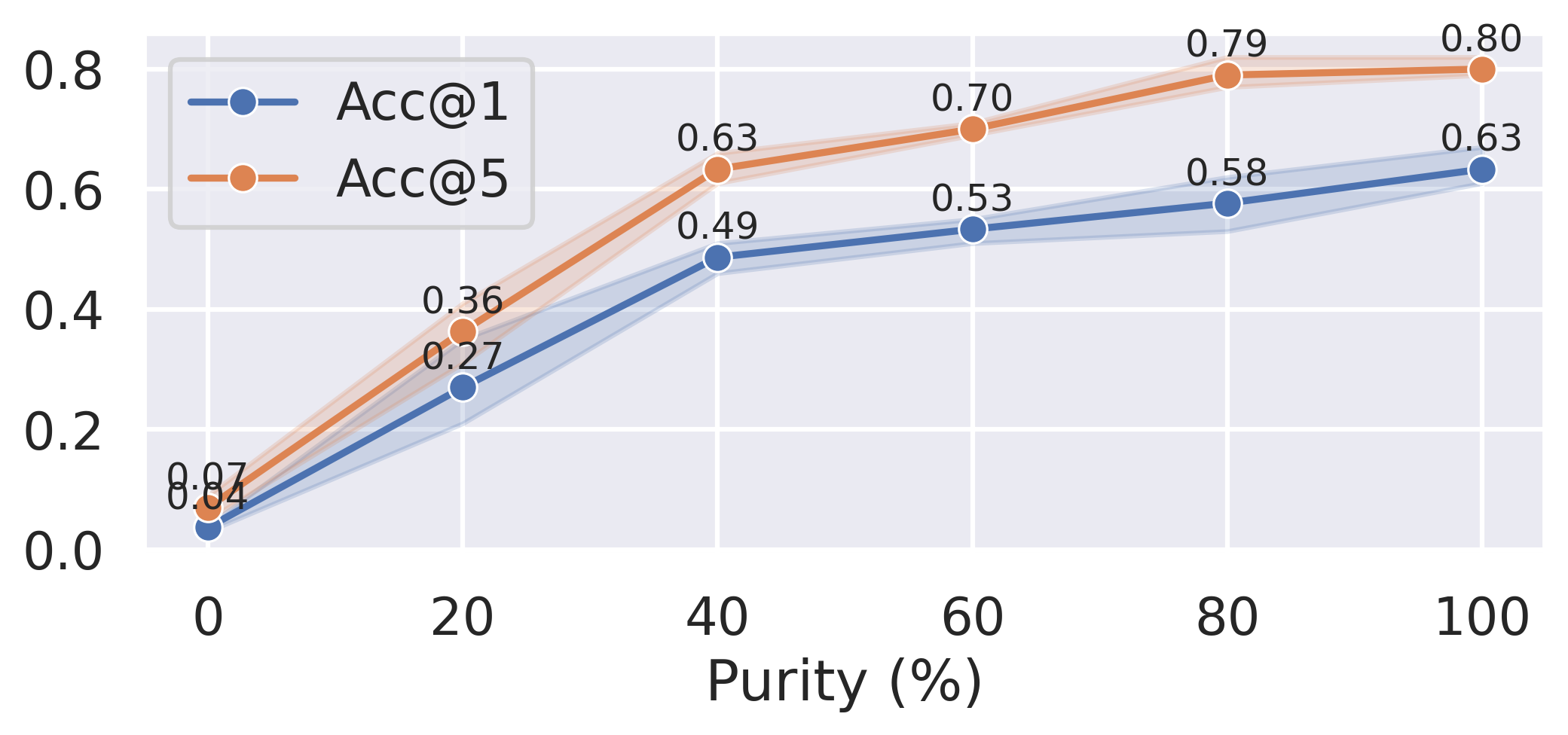
In the VisDiffBench dataset, image sets are composed with perfect purity. For instance, $\mathcal{D}_{A}$ exclusively contains cat images (100%), while $\mathcal{D}_{B}$ is entirely made up of dog images (100%). However, this level of purity is rare in real-world scenarios. Typically, such sets include a mix of elements – for example, $\mathcal{D}_{A}$ might comprise 70% cat images and 30% dog images, and $\mathcal{D}_{B}$ vice versa. To evaluate the robustness of the VisDiff algorithm against such noise, we introduced randomness in VisDiffBench by swapping a certain percentage of images between $\mathcal{D}_{A}$ and $\mathcal{D}_{B}$. Here, 0% purity signifies 50% image swapping and an equal distribution of two sets, whereas 100% purity indicates no image swapping.

Figure 4 presents the Acc@1 and Acc@5 performance of VisDiff across various purity levels, tested on 50 paired sets within PairedImageSets-Hard. As anticipated, a decline in purity correlates with a drop in accuracy since identifying the difference becomes harder. However, even at 40% purity, Acc@1 remains at 49%, only modestly reduced from 63% at 100% purity. This result underscores the robustness of the VisDiff algorithm to noisy data. It is also worth noting that VisDiff reaches near 0% accuracy at 0% purity, which is expected since the two sets have exactly the same distribution and our method filters out invalid differences.

Other ablations of VisDiff algorithm.

In Appendix C, we further discuss how caption style, language model, sample size, and # sampling rounds affect VisDiff performance.

Figure 4: VisDiff performance under noise. We randomly swap different percentages of images between $\mathcal{D}_{A}$ and $\mathcal{D}_{B}$ to inject noise. Results are computed on 50 paired sets in PairedImageSets-Hard. 95% confidence intervals are reported over three runs.

6 Applications

We apply the best configuration of our VisDiff method to a set of five applications in computer vision: 1) comparing ImageNet and ImageNetV2 (Section 6.1), 2) interpreting the differences between two classifiers at the datapoint level (Section 6.2), 3) analyzing model errors (Section 6.3), 4) understanding the distributional output differences between StableDiffusionV1 and V2 (Section 6.4), and 5) discovering what makes an image memorable (Section 6.5). Since VisDiff is automatic, we used it to discover differences between (1) large sets of images or (2) many sets of images, thus mass-producing human-interpretable insights across these applications. In this section, we report VisDiff-generated insights including some that can be confirmed with existing work and others that may motivate future investigation in the community. Additional details for each application can be found in Appendix D.

6.1 Comparing ImageNetV2 with ImageNet

In 2019, a decade after ImageNet [5] was collected, Recht et al. introduced ImageNetV2 [35], which attempted to mirror the original ImageNet collection process, including restricting data to images uploaded in a similar timeframe. However, models trained on ImageNet showed a consistent 11-14% accuracy drop on ImageNetV2, and the reasons for this have remained unclear. While some studies have employed statistical tools to reveal a distributional difference between ImageNet and ImageNetV2 [10], we aim to discover more interpretable differences between these two datasets.

To uncover their differences, we first ran VisDiff with $\mathcal{D}_{A}$ as all of ImageNetV2 images and $\mathcal{D}_{B}$ as all of ImageNet images. Interestingly, the highest scoring description generated by our system is “photos taken from Instagram”. We conjecture that this highlights temporal distribution shift as a potential reason behind model performance drops on ImageNetV2 vs V1. Indeed, while ImageNetV2 aimed to curate images uploaded in a similar timeframe to ImageNet, all images in ImageNet were collected prior to 2012 whereas a portion of ImageNetV2 was collected between 2012 and 2014 [35]. This shift in years happens to coincide with the explosion of social media platforms such as Instagram, which grew from 50M users in 2012 to 300M users in 2014 [7]. In this case, we hypothesize that a small difference in the time range had a potentially outsized impact on the prevalence of Instagram-style photos in ImageNetV2 and the performance of models on this dataset.

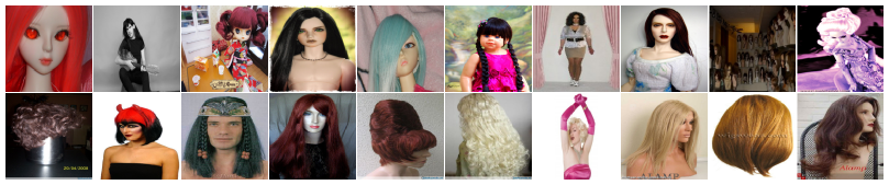
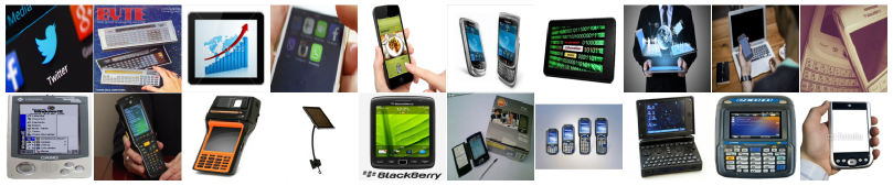
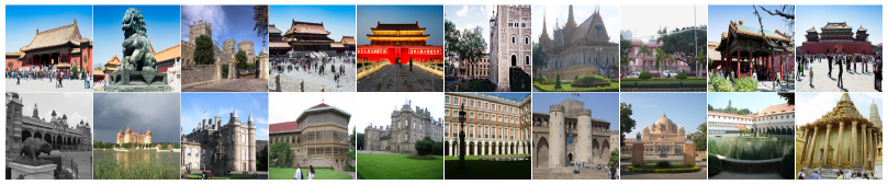
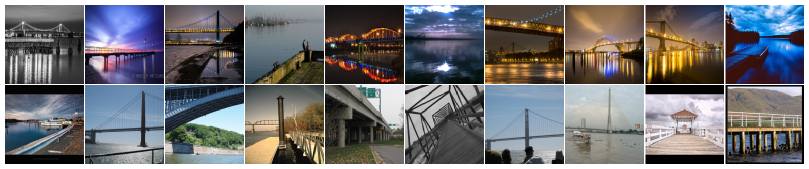
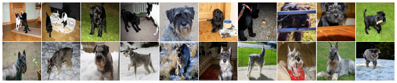
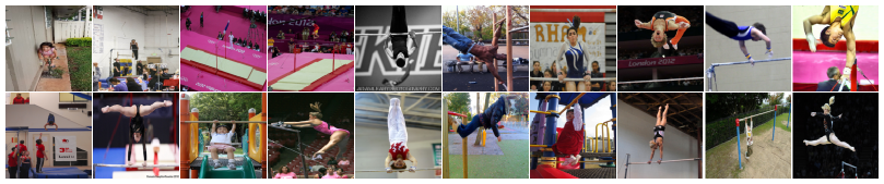
Beyond dataset-level analysis, we applied VisDiff to each of the 1,000 ImageNet classes, comparing ImageNetV2 images ($\mathcal{D}_{A}$) against ImageNet images ($\mathcal{D}_{B}$). Notable class-specific differences are listed in Table 3, ranked by difference score, with visualizations in Figure 13. Several of these differences suggest more specific examples of Instagram-style photos, consistent with our dataset-level finding. For example, for the class “Dining Table”, ImageNetV2 contains substantially more images showing “people posing for a picture”, visualized in Figure 1. For the class “Horizontal Bar”, ImageNetV2 is also identified to have more images of “men’s gymnastics events.” Upon manual inspection, we find that this highlights the difference that ImageNetV2 happens to contain photographs of the Men’s High Bar gymnastics event in the 2012 Olympics, which occurred after the ImageNet collection date. These examples illustrate how VisDiff can be used as a tool for surfacing salient differences between datasets.

Class	More True for ImageNetV2
Dining Table	People posing for a picture
Wig	Close up views of dolls
Hand-held Computer	Apps like Twitter and Whatsapp
Palace	East Asian architecture
Pier	Body of water at night
Schnauzer	Black dogs in different settings
Pug	Photos possibly taken on Instagram
Horizontal Bar	Men’s gymnastics events

Table 3: Top per-class differences between ImageNet and V2.

6.2 Comparing Behaviors of CLIP and ResNet

In 2021, OpenAI’s CLIP [34] showcased impressive zero-shot object recognition, matching the fully supervised ResNet [13] in ImageNet accuracy while showing a smaller performance drop on ImageNetV2. Despite similar in-distribution performance on ImageNet, CLIP and ResNet differ in robustness [29]. This naturally leads to two questions: 1) do these models make similar predictions on individual datapoints in ImageNet? 2) on what datapoints does CLIP perform better than ResNet in ImageNetV2?

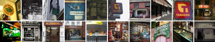
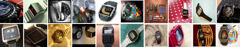
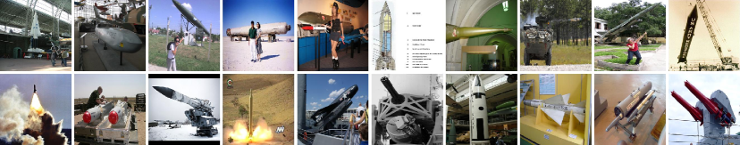
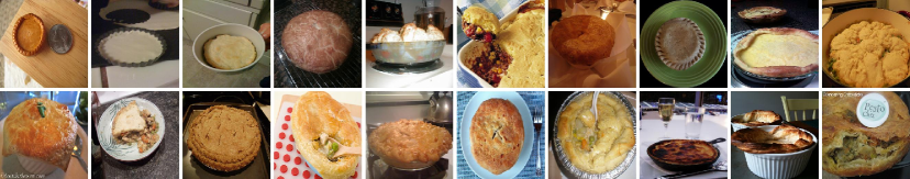
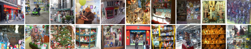
To investigate these questions, we analyzed ResNet-50 and zero-shot CLIP ViT-H, which achieve similar accuracies of 75% and 72% on ImageNet, respectively. To study the first question, VisDiff was applied to the top 100 classes where CLIP surpasses ResNet. $\mathcal{D}_{A}$ comprised images correctly identified by CLIP but not by ResNet, and $\mathcal{D}_{B}$ included all other images. The top discoveries included “close-ups of everyday objects”, “brands and specific product labeling”, and “people interacting with objects”. The first two align well with existing works that show CLIP is robust to object angles and sensitive to textual elements (e.g., a fruit apple with text “iPod” on it will be misclassified as “iPod”) [34, 12]. In addition, we ran VisDiff at finer granularity on each of the top 5 classes where CLIP outperforms ResNet. The discovered class-level differences are shown in Table 4, demonstrating CLIP’s proficiency in identifying “tobacco shops with signs”, “group displays of digital watches”, and “scenes involving missiles and toyshops with human interactions”, which echos the dataset-level findings about label, object angle, and presence of people.

Class	AccC	AccR	More Correct for CLIP
Tobacco Shop	0.96	0.50	Sign hanging from the side of a building
Digital Watch	0.88	0.52	Watches displayed in a group
Missile	0.78	0.42	People posing with large missiles
Pot Pie	0.98	0.66	Comparison of food size to coins
Toyshop	0.92	0.60	People shopping in store

Table 4: Top per-class differences between CLIP and ResNet. Acc_C and $Acc_{R}$ are accuracy of CLIP and ResNet, respectively.

To study the second question, we applied VisDiff to ImageNetV2’s top 100 classes where CLIP outperforms ResNet. We set $\mathcal{D}_{A}$ as images where CLIP is correct and ResNet is wrong, and $\mathcal{D}_{B}$ as the rest. The top three differences are: 1) “Interaction between humans and objects”, suggesting CLIP’s robustness in classifying images with human presence; 2) “Daytime outdoor environments”, indicating CLIP’s temporal robustness; and 3) “Group gatherings or social interactions”, which is similar to the first difference. These findings provide insight into CLIP’s strengths versus ResNet on ImageNetV2, and are also consistent with the findings in Section 6.1 that ImageNetV2 contains more social media images with more presence of people.

Figure 5: StableDiffusionV2 vs. V1 generated images. For the same prompt, StableDiffusionV2 images often contain more “vibrant contrasting colors” and “artworks placed on stands or in frames”. Randomly sampled images can be found in Figure 16.

6.3 Finding Failure Modes of ResNet

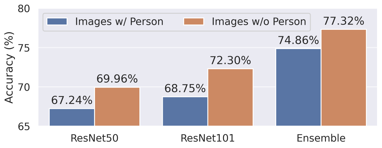
We utilize VisDiff to identify failure modes of a model by contrasting images that are correctly predicted against those that are erroneously classified. Using a ResNet-50 and ResNet-101 [13] trained on ImageNet, we set $\mathcal{D}_{A}$ as ImageNet images misclassified by both ResNet-50 and ResNet-101 and $\mathcal{D}_{B}$ as correctly classified images. The two highest scoring descriptions were “humanized object items” and “people interacting with objects”, suggesting that ResNet models perform worse when the images include human subjects, echoing the finding in Section 6.2.

To validate this hypothesis, we applied a DETR [36] object detector to find a subset of ImageNet images with human presence. Using the classes which have a roughly equal number of human/no-human images, we evaluated ResNets on this subset and their accuracy indeed declined 3-4%, as shown in Figure 6.

Figure 6: Accuracy on images with / without people.

6.4 Comparing Versions of Stable Diffusion

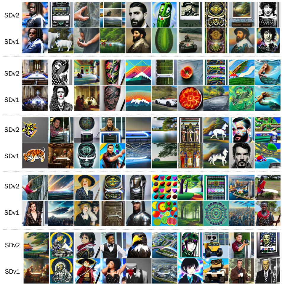
In 2022, Stability AI released StableDiffusionV1 (SDv1), followed by StableDiffusionV2 (SDv2) [38]. While SDv2 can be seen as an update to SDv1, it raises the question: What are the differences in the images produced by these two models?

Using the prompts from PartiPrompts [47] and DiffusionDB [45], we generated 1634 and 10000 images with SDv2 and SDv1, respectively. The Parti images are used to propose differences and the DiffusionDB images are used to validate these differences transfer to unseen prompts.

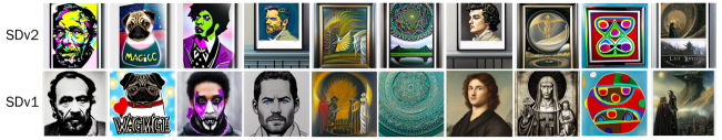
The top differences show that SDv2 produces more “vibrant and contrasting colors” and interestingly “images with frames or borders” (see Table 7). We confirmed the color difference quantitatively by computing the average saturation: 112.61 for SDv2 versus 110.45 for SDv1 from PartiPrompts, and 97.96 versus 93.49 on unseen DiffusionDB images. Qualitatively, as shown in Section Figure 5, SDv2 frequently produces images with white borders or frames, a previously unknown characteristic. This is further substantiated in Section Appendix D, where we employ edge detection to quantify white borders, providing 50 random image samples from both SDv1 and SDv2.

6.5 Describing Memorability in Images

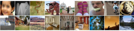
Finally, we demonstrate the applicability of VisDiff in addressing diverse real-world questions beyond machine learning, such as computational cognitive science. A key area of interest, especially for photographers and advertisers, is enhancing image memorability. Isola et al. [16] explored this question and created the LaMem dataset, where each image is assigned a memorability score by humans in the task of identifying repeated images in a sequence.

Applying VisDiff to the LaMem dataset, we divided images into two groups: $\mathcal{D}_{A}$ (the most memorable 25th percentile) and $\mathcal{D}_{B}$ (the least memorable 25th percentile). Our analysis found that memorable images often include “presence of humans”, “close-up views”, and “humorous settings”, while forgettable ones feature “landscapes” and “urban environments”. These findings are consistent with those of Isola et al. [16], as further detailed qualitatively in Figure 7 and quantitatively in Appendix D.

Figure 7: Memorable(top) vs. forgettable(bottom) images. Memorable images contain more “humans”, “close-up views of body part or objects”, and “humorous settings”, while forgettable images contain more “landscapes” and “urban environments”

7 Conclusion

In this work, we introduce the task of set difference captioning and develop VisDiff, an algorithm designed to identify and describe differences in image sets in natural language. VisDiff first uses large language models to propose differences based on image captions and then employs CLIP to effectively rank these differences. We rigorously evaluate VisDiff’s various design choices on our curated VisDiffBench, and show VisDiff’s utility in finding interesting insights across a variety of real-world applications.

Limitations.

As we see in Section 5, VisDiff still has a large room for improvement and hence far from guaranteed to uncover all meaningful differences. Furthermore, VisDiff is meant to be an assistive tool for humans to better understand their data and should not be applied without a human in the loop: the users hold the ultimate responsibility to interpret the descriptions by VisDiff properly. As VisDiff relies heavily on CLIP, GPT, and BLIP, any biases or errors these models may extend to VisDiff. Further investigation of VisDiff’s failure cases can be found in Appendix E.

Supplementary Material

Reproducibility Statement

We provide code implementations of VisDiff at https://github.com/Understanding-Visual-Datasets/VisDiff. We also provide VisDiffBench at https://drive.google.com/file/d/1vghFd0rB5UTBaeR5rdxhJe3s7OOdRtkY. The implementations and datasets will enable researchers to reproduce all the experiments described in the paper as well as run their own analyses on additional datasets.

Ethics Statement

In this work, we introduce VisDiff, a novel method designed to discern subtle differences between two sets of images. VisDiff represents not just a technical advance in the analysis of image sets, but also serves as a useful tool to promote fairness, diversity, and scientific discovery in AI and data science. First, VisDiff has the potential to uncover biases in datasets. For instance, comparing image sets of workers from diverse demographic groups, such as men and women, can reveal and quantify career stereotypes associated with each group. This capability is pivotal in addressing and mitigating biases present in datasets. Furthermore, VisDiff holds substantial promise for scientific discovery. By comparing image sets in various scientific domains, such as cellular images from patients and healthy individuals, VisDiff can unveil novel insights into the disease impacts on cellular structures, thereby driving forward critical advancements in medical research. However, VisDiff is meant to be an assistive tool and should be applied with humans in the loop. The users are responsible for interpreting the results properly and avoiding misinformation. In summary, VisDiff emerges as a crucial tool for ethical AI considerations, fostering fairness and catalyzing scientific progress.

Table of Contents

In this supplementary material, we provide additional details of datasets, methods, results, and applications.

• In Appendix A, we provide examples of our benchmark VisDiffBench and prompts to generate and evaluate this benchmark.

• In Appendix B, we provide additional details of each proposer and ranker.

• In Appendix C, we ablate various design choices of our algorithm VisDiff.

• In Appendix D, we provide supplementary evidence of findings for each application.

• In Appendix E, we explain more failure cases and limitations of VisDiff.

Appendix A Supplementary Section 3

In this section, we provide additional details of Section 3 in the main paper.

A.1 Paired Sentences for VisDiffBench

VisDiffBench contains five subsets: PairedImageSets-Easy, PairedImageSets-Medium, PairedImageSets-Hard, ImageNetR, and ImageNet^∗. We provide all the paired sentences of PairedImageSets in Table 5. For ImageNetR, $\mathcal{D}_{A}$ is one of the “art”, “cartoon”, “deviantart”, “embroidery”, “graffiti”, “graphic”, “origami”, “painting”, “sculpture”, “sketch”, “sticker”, “tattoo”, “toy”, “videogame”, and $\mathcal{D}_{B}$ is “imagenet”. For ImageNet^∗, $\mathcal{D}_{A}$ is one of the “in the forest”, “green”, “red”, “pencil sketch”, “oil painting”, “orange”, “on the rocks”, “in bright sunlight”, “person and a”, “in the beach”, “studio lighting”, “in the water”, “at dusk”, “in the rain”, “in the grass”, “yellow”, “blue”, “and a flower”, “on the road”, “at night”, “embroidery”, “in the fog”, “in the snow”, and $\mathcal{D}_{B}$ is “base”.

Easy (50 Paired Sets)		Medium (50 Paired Sets)		Hard (50 Paired Sets)
Set A	Set B	Set A	Set B	Set A	Set B
Dogs playing in a park	Cats playing in a park	SUVs on a road	Sedans on a road	Sunrise over Santorini, Greece	Sunset over Santorini, Greece
Children playing soccer	Children swimming in a pool	Wooden chairs in a room	Plastic chairs in a room	People practicing yoga in a mountainous setting	People meditating in a mountainous setting
Snow-covered mountains	Desert sand dunes	Golden retriever dogs playing	Labrador dogs playing	Fresh sushi with salmon topping	Fresh sushi with tuna topping
Butterflies on flowers	Bees on flowers	Green apples in a basket	Red apples in a basket	Lush vineyards in spring	Lush vineyards in early autumn
People shopping in a mall	People dining in a restaurant	Leather shoes on display	Canvas shoes on display	Men wearing Rolex watches	Men wearing Omega watches
Elephants in the savannah	Giraffes in the savannah	Freshwater fish in an aquarium	Saltwater fish in an aquarium	Cupcakes topped with buttercream	Cupcakes topped with fondant
Birds flying in the sky	Airplanes flying in the sky	Steel bridges over a river	Wooden bridges over a river	People playing chess outdoors	People playing checkers outdoors
Boats in a marina	Cars in a parking lot	Mountain bikes on a trail	Road bikes on a road	Hand-painted porcelain plates	Hand-painted ceramic plates
Tulips in a garden	Roses in a garden	Ceramic mugs on a shelf	Glass mugs on a shelf	Cyclists in a time-trial race	Cyclists in a mountain stage race
People skiing on a slope	People snowboarding on a slope	People playing electric guitars	People playing acoustic guitars	Gardens with Japanese cherry blossoms	Gardens with Japanese maples
Fish in an aquarium	Turtles in an aquarium	Laptop computers on a desk	Desktop computers on a desk	People wearing traditional Korean hanboks	People wearing traditional Japanese kimonos
Books on a shelf	Plants on a shelf	Hardcover books on a table	Paperback books on a table	Alpine lakes in summer	Alpine lakes in early spring
Grapes in a bowl	Apples in a bowl	Digital clocks on a wall	Analog clocks on a wall	Merlot wine in a glass	Cabernet Sauvignon wine in a glass
Motorcycles on a street	Bicycles on a street	Children playing with toy cars	Children playing with toy trains	Football players in defensive formation	Football players in offensive formation
Cows grazing in a field	Sheep grazing in a field	White roses in a vase	Pink roses in a vase	Classic novels from the 19th century	Modern novels from the 21st century
Babies in cribs	Babies in strollers	Electric stoves in a kitchen	Gas stoves in a kitchen	Orchestras playing Baroque music	Orchestras playing Classical music
Hot air balloons in the air	Kites in the air	Leather jackets on hangers	Denim jackets on hangers	Men in British army uniforms from WWI	Men in British army uniforms from WWII
Penguins in the snow	Seals in the snow	People eating with chopsticks	People eating with forks	Sculptures from the Renaissance era	Sculptures from the Hellenistic era
Lions in a jungle	Monkeys in a jungle	Pearl necklaces on display	Gold necklaces on display	People preparing macarons	People preparing meringues
Watches on a display	Rings on a display	Mushrooms in a forest	Ferns in a forest	Female ballet dancers in pointe shoes	Female ballet dancers in ballet slippers
Pizzas in a box	Donuts in a box	Stainless steel kettles in a store	Plastic kettles in a store	Dishes from Northern Italian cuisine	Dishes from Southern Italian cuisine
Bricks on a wall	Tiles on a wall	Porcelain vases on a shelf	Metal vases on a shelf	Classic rock bands performing	Alternative rock bands performing
Pianos in a room	Guitars in a room	Vintage cars on a road	Modern cars on a road	Historical films set in Medieval Europe	Historical films set in Ancient Rome
Trains on tracks	Buses on roads	Handmade quilts on a bed	Factory-made blankets on a bed	Bonsai trees shaped in cascade style	Bonsai trees shaped in informal upright style
Pots on a stove	Plates on a table	Shiny silk dresses on mannequins	Matte cotton dresses on mannequins	Lace wedding dresses	Satin wedding dresses
Stars in the night sky	Clouds in the day sky	Mechanical pencils on a desk	Ballpoint pens on a desk	Birds with iridescent plumage	Birds with matte plumage
Sunflowers in a field	Wheat in a field	Ginger cats lying down	Tabby cats lying down	Women wearing matte lipstick	Women wearing glossy lipstick
Dolls on a shelf	Teddy bears on a shelf	People riding racing horses	People riding dressage horses	Cities with Gothic architecture	Cities with Modernist architecture
Pine trees in a forest	Oak trees in a forest	Steel water bottles on a table	Glass water bottles on a table	Poems written in free verse	Poems written in sonnet form
Men playing basketball	Women playing volleyball	Men wearing leather gloves	Men wearing wool gloves	Acoustic guitars being played	Classical guitars being played
Ice cream in a cone	Juice in a glass	Rubber ducks in a tub	Plastic boats in a tub	Books with hardcover binding	Books with leather-bound covers
Dancers on a stage	Singers on a stage	Porcelain tea cups on a tray	Glass tea cups on a tray	Portraits painted in cubist style	Portraits painted in impressionist style
Rainbows in the sky	Lightning in the sky	Sparrows on a tree	Canaries on a tree	Residential buildings in Art Deco style	Residential buildings in Brutalist style
Towers in a city	Houses in a suburb	Shiny metallic cars	Matte finish cars	Male professional swimmers in freestyle race	Male professional swimmers in butterfly race
Frogs by a pond	Ducks by a pond	Stuffed teddy bears on a bed	Stuffed bunny rabbits on a bed	Basketball players attempting free throws	Basketball players attempting slam dunks
Football players on a field	Rugby players on a field	Round dinner plates on a table	Square dinner plates on a table	Cakes decorated with marzipan	Cakes decorated with buttercream roses
Pillows on a bed	Blankets on a bed	Butter on a slice of bread	Jam on a slice of bread	People practicing the Sun Salutation in yoga	People practicing the Tree Pose in yoga
Deer in a forest	Rabbits in a forest	Bengal cat in sitting posture	Siamese cat in sitting posture	Men wearing suits	Men wearing tuxedos
Tea in a cup	Coffee in a cup	Violinists playing in a quartet	Cellists playing in a quartet	Butterflies with spotted wings	Butterflies with striped wings
Children on a slide	Children on a swing	Gothic cathedrals in Europe	Baroque churches in Europe	Oak trees in summer	Oak trees in autumn
Kangaroos in a desert	Camels in a desert	People dancing tango	People dancing waltz	Tennis shoes on a rack	Running shoes on a rack
Tomatoes in a basket	Eggs in a basket	Abstract oil paintings with warm colors	Abstract oil paintings with cool colors	People playing classical violin	People playing fiddle
People in an elevator	People on an escalator	Candies made from dark chocolate	Candies made from milk chocolate	Men wearing fedoras	Men wearing baseball caps
Sandcastles on a beach	Umbrellas on a beach	Rivers in tropical rainforests	Rivers in alpine meadows	Passenger planes in the sky	Cargo planes in the sky
Mice in a barn	Horses in a barn	Cars from the 1960s	Cars from the 1980s	Women wearing ankle boots	Women wearing knee-high boots
Chocolates in a box	Candies in a jar	Seascapes during a storm	Seascapes during a calm day	Diesel trucks on a highway	Electric trucks on a highway
Zebra crossings on a street	Traffic lights on a street	Fruits arranged in a still life setting	Flowers arranged in a still life setting	Children reading comic books	Children reading fairy tales
Bridges over a river	Boats on a river	Dishes from Thai cuisine	Dishes from Vietnamese cuisine	Men wearing round glasses	Men wearing square glasses
Oranges on a tree	Bird nests on a tree	Wild horses in American plains	Wild zebras in African savannahs	Vinyl records in a store	CDs in a store
Lanterns in a festival	Fireworks in a festival	Classic movies in black and white	Classic movies in Technicolor	Bonsai trees in pots	Cacti in pots

Table 5: Paired sentences for PairedImageSets. Easy, medium, and hard examples are shown in the left, middle, and right.

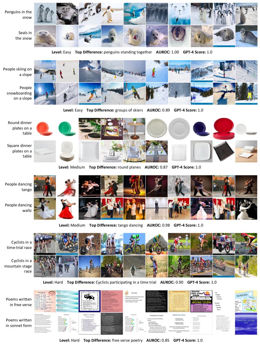
A.2 Examples for VisDiffBench

We provide 4 examples for PairedImageSets-Easy, PairedImageSets-Medium, PairedImageSets-Hard, respectively, in Figure 8 and Figure 17. For ImageNetR and ImageNet^∗, we refer readers to the original papers [14, 43].

Figure 8: PairedImageSets examples where VisDiff succeeds. We show the ground-truth difference, top difference predicted by VisDiff, AUROC score output by the ranker, and evaluation of the predicted difference by GPT-4.

A.3 Prompts for VisDiffBench Generation

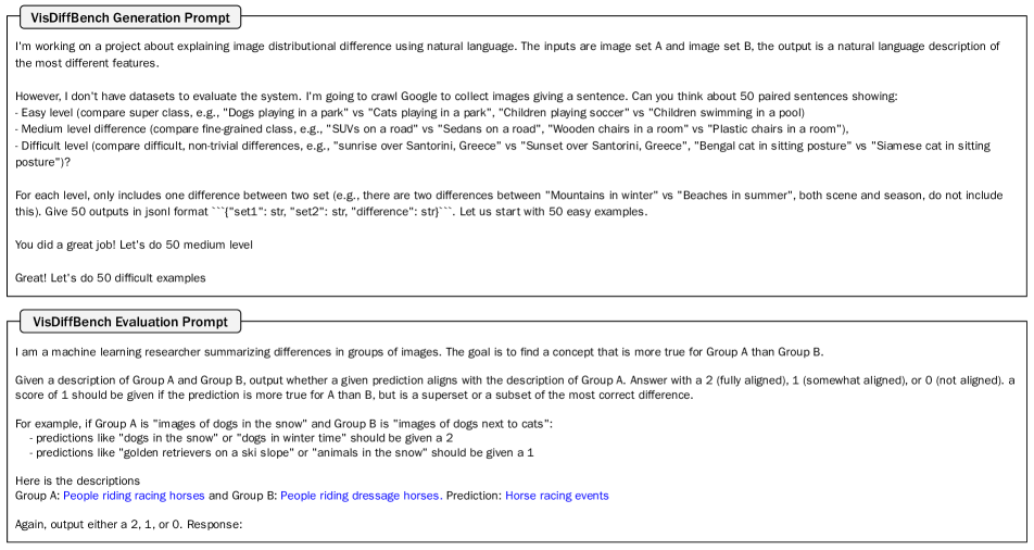
We provide the GPT-4 prompt we used to generate paired sentences for PairedImageSets in Figure 9 (top).

A.4 Prompts for VisDiffBench Evaluation

We provide the GPT-4 prompt we used to evaluate the generated difference description against the ground-truth difference description in Figure 9 (bottom).

Figure 9: Prompt used to generate paired sentences for VisDiffBench (top) and evaluate VisDiffBench (bottom). Input-dependent texts are colored in blue.

Appendix B Supplementary Section 4

In this section, we provide additional details of Section 4 in the main paper.

B.1 Details for Proposer

We ran each proposer for 3 rounds. For each round, we sample 20 examples per set and generate 10 hypotheses.

Image-based Proposer.

We provide an example input of the gridded image in Figure 10. We feed the image and the prompt shown in Figure 11 (middle) to LLaVA-1.5 to generate 10 hypotheses.

Figure 10: Example input to the image-based proposer. We arrange 20+20 input images into a single 4-row, 10-column gridded image.

Feature-based Proposer.

To generate 10 hypotheses, we sample BLIP-2 10 times using top-p sampling given the subtracted embedding.

Caption-based Proposer.

We generate captions for each image using BLIP-2 with the prompt “Describe this image in detail.”. We apply a simple filtering of the captions, which removes any special tokens and captions simply repeating words. We feed the filtered captions and the prompt shown in Figure 11 (top) to GPT-4 to generate 10 hypotheses.

B.2 Details for Ranker

Image-based Ranker.

Given each hypothesis, we prompt LLaVA-1.5 with the image and the prompt “Does this image contain {hypothesis}?”.

Caption-based Ranker.

Given each hypothesis, we prompt Vicuna-1.5 with the image caption and hypothesis using the prompt shown in Figure 11 (bottom).

Feature-based Ranker.

We use the OpenCLIP model ViT-bigG-14 trained on laion2b_s39b_b160k.

Appendix C Supplementary Section 5

In this section, we provide additional details of Section 5 in the main paper. We ablate various design choices of VisDiff.

Figure 11: Prompt for caption-based proposer (top), image-based proposer (middle), and caption-based ranker (bottom). Input-dependent texts are colored in blue.

Proposer	Ranker	PIS-Easy		PIS-Medium		PIS-Hard		ImageNet-R/*
		Acc@1	Acc@5	Acc@1	Acc@5	Acc@1	Acc@5	Acc@1	Acc@5
GPT-4 on BLIP-2 Captions	CLIP	0.88	0.99	0.75	0.86	0.61	0.80	0.78	0.96
GPT-4 on LLaVA-1.5 Captions	CLIP	0.89	0.98	0.73	0.85	0.51	0.70	0.84	0.93
GPT-3.5 on BLIP-2 Captions	CLIP	0.81	0.95	0.67	0.87	0.60	0.76	0.85	0.96

Table 6: Results on VisDiffBench with different captions and language models. We bold any numbers within 0.02.

Figure 12: Analysis of the number of rounds (left) and number of samples (right) for the proposer on 50 PairedImageSets-Hard sets. 3 rounds and 20 samples are the best in terms of performance and efficiency.

C.1 Caption Styles

Given that our leading proposer is caption-based, it naturally raises the question of how captions derived from vision language models influence performance. We conducted a comparative analysis of captions generated by two state-of-the-art vision language models: BLIP-2 and LLaVA-1.5. Notably, compared to BLIP-2, LLaVA-1.5 has been instruction-tuned and can produce captions that are much longer with detailed information. The average caption length for LLaVA is around 391 characters compared to BLIP-2’s 41 characters. As shown in Table 6, despite the clear disparity between these two captions, the algorithm achieves similar performances. This suggests that language models possess a robust inductive reasoning ability that allows them to discern the most notable differences in language. BLIP-2’s captions, being marginally superior, could be attributed to their shortness and conciseness.

C.2 Language Models

We compared GPT-4 with GPT-3.5 in Table 6 to assess how different language models affect the caption-based proposer. While both models achieve strong performances on VisDiffBench, GPT-4 outperforms GPT-3.5 in most cases, demonstrating that the stronger reasoning capability of language models is important to accomplish the set difference captioning task.

C.3 Sampling Rounds

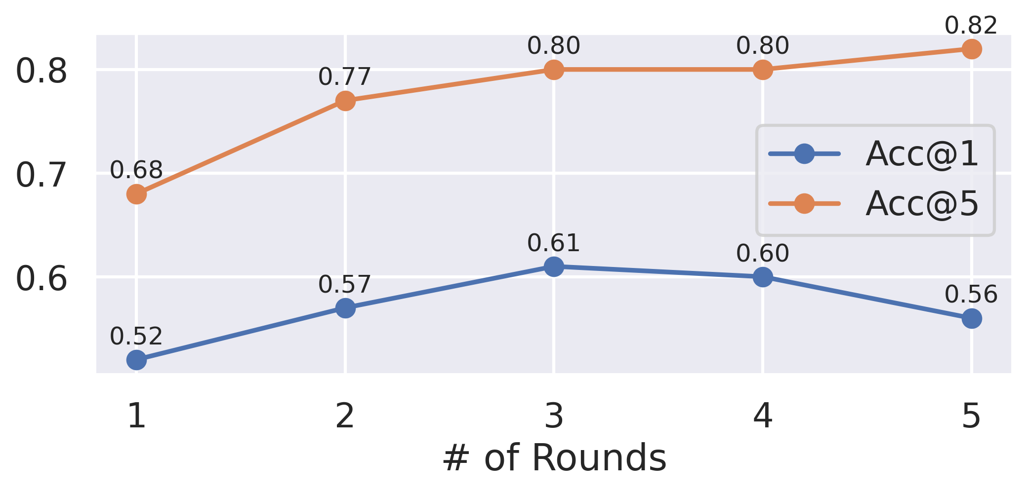
The proposer’s generated differences rely on the random samples drawn from each image set; thus, extensive sampling is paramount to capture all the differences. Our ablation studies presented in Figure 12 (left), conducted on the PairedImageSets hard subset, suggest that an increase in sampling iterations typically correlates with enhanced performance. However, a point of diminishing returns is observed beyond three rounds of proposals. In this paper, we standardize the experiments based on three rounds of proposal generation.

C.4 Number of Sampled Examples

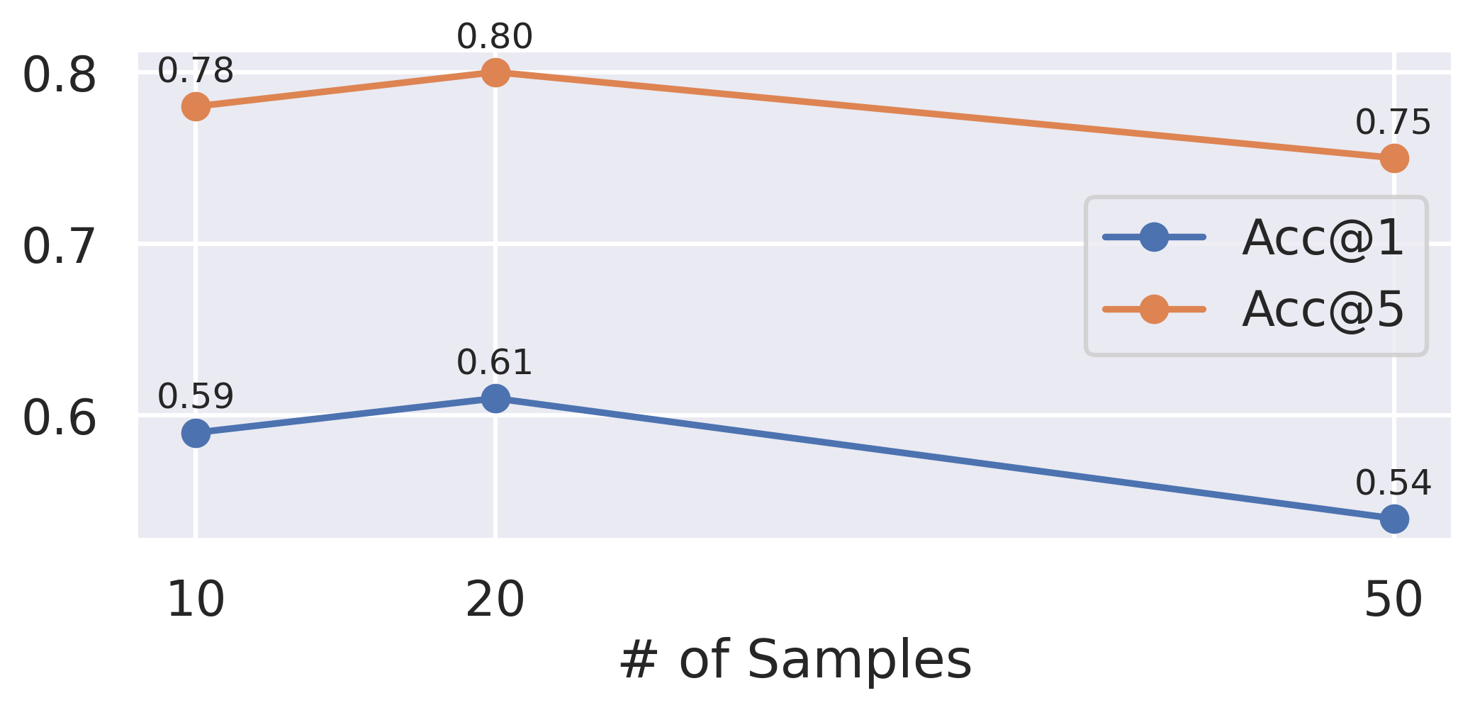
Inputting more samples from $\mathcal{D}_{A}$ and $\mathcal{D}_{B}$ into the proposer may not be advantageous, as a long context could result in information getting lost in the middle [26, 40]. Results shown in Figure 12 (right) reflect this, as inputting more captions to the large language models sees performance benefits up to 20 captions, at which point performance degrades.

C.5 Necessity of Ranker

Since the proposer may already generate and sort the most salient difference descriptions based on the sampled images, we conduct ablations to understand whether the ranker is necessary. We observe that, on PairedImageSets hard subset, VisDiff achieves 0.54 Acc@1 and 0.68 Acc@5 without ranker, which is much lower than the 0.61 Acc@1 and 0.80 Acc@5 with ranker, demonstrating the necessity of the ranker.

Appendix D Supplementary Section 6

In this section, we provide additional details of Section 6 in the main paper.

D.1 Comparing ImageNetV2 with ImageNet

Per-class visualizations.

Along with the “Dinner Table” example shown in Figure 1, we provide other per-class differences with the highest difference scores in Figure 13. These examples clearly reveal salient differences between ImageNetV2 and ImageNet. Moreover, we observe time differences between these two datasets, as ImageNetV2 images contain Twitter and WhatsApp in the “Hand-held Computer” class and London 2012 Oylmpics in the “Horizontal Bar” class.

(a) Wig    Diffs: “Close up views of dolls”, “Japanese style dolls”, “Images including Barbie dolls”

(b) Hand-held Computer    Diffs: “Apps like Twitter and Whatsapp”, “Digital devices with green screen”, “Interconnection between laptop and smart phone”

(c) Palace    Diffs: “East Asian architecture”, “Images featuring the Forbidden City in Beijing”, “Images including red buildings with Chinese writing”

(d) Pier    Diffs: “Body of water at night”,“Urban night skyline”, “Long exposure shots”

(e) Schnauzer    Diffs: “Black dogs in different settings”, “Terrier puppies with objects”, “Interaction with different objects”

(f) Horizontal Bar    Diffs: “Men’s gymnastics events”, “London 2012 Olympics”, “Gymnastics event in 2013”

Figure 13: ImageNetV2 vs. ImageNet. All V2 images are shown in the first row while V1 images are shown in the second row. We show the class name and top 3 difference descriptions generated by VisDiff.

ImageNetV2 metadata analysis.

To get more precise statistics on when the ImageNetV2 images were collected, we analyzed the metadata of each image, which reports the minimum and maximum upload date of that image to Flickr. We find that 72% images were uploaded between 2012 and 2013, and 28% were uploaded between 2013 and 2014. This is different from ImageNet images that were all collected on or before 2010.

D.2 Comparing Behaviors of CLIP and ResNet

Per-class visualizations.

We provide per-class differences where CLIP outperforms ResNet most in Figure 14. These examples clearly reveal salient differences between CLIP and ResNet, such as CLIP’s robustness to label within images, object angle, and presence of people.

(a) Tobacco Shop    Diffs: “Sign hanging from the side of a building”, “Falcon images”,“Presence of street signs”

(b) Digital Watch    Diffs: “Watches displayed in a group”,“Arrangement of multiple watches”,“Watches with colored straps”

(c) Missile    Diffs: “People posing with large missiles”,“people posing with rockets”,“missiles on display”

(d) Pot Pie    Diffs: “Comparison of food size to coins”,“Utilization of cutting board”,“Inclusion of beverages”

(e) Toy Shop    Diffs: “People shopping in store”,“Female customer in store”,“Specific location based scene”

Figure 14: CLIP vs. ResNet. All CLIP correctly classified but ResNet incorrectly classified images are shown in the first row while other images are shown in the second row. We show the class name and top 3 difference descriptions generated by VisDiff.

D.3 Finding Failure Modes of ResNet

Model details.

We use the PyTorch pre-trained ResNet-50 and ResNet-101 models and the Huggingface “facebook/detr-resnet-50” object detector.

Top differences.

The top 5 difference descriptions from VisDiff were “humanized object items”, “people interacting with objects”, “electronics and appliances”, “objects or people in a marketplace setting”, and “household objects in unusual placement”.

D.4 Comparing Versions of Stable Diffusion

Figure 15: Modified proposer’s prompt for StableDiffusion analysis.

Text-to-image generation details.

We use the Huggingface models “CompVis/stable-diffusion-v1-4” and “stabilityai/stable-diffusion-2-1” with guidance of 7.5 and negative prompts “bad anatomy, bad proportions, blurry, cloned face, cropped, deformed, dehydrated, disfigured, duplicate, error, extra arms, extra fingers, extra legs, extra limbs, fused fingers, gross proportions, jpeg artifacts, long neck, low quality, lowres, malformed limbs, missing arms, missing legs, morbid, mutated hands, mutation, mutilated, out of frame, poorly drawn face, poorly drawn hands, signature, text, too many fingers, ugly, username, watermark, worst quality”.

VisDiff details.

Unlike the previous applications, there exists a one-to-one mapping between $\mathcal{D}_{A}$ and $\mathcal{D}_{B}$ through the generation prompt. Therefore, we modify the subset sampling process to include the images generated from the same prompts and modify the proposer’s prompt to include the generation prompts (Figure 15). We used LLaVA-1.5 for captioning rather than BLIP-2 because we were particularly interested in the details of the images.

Top differences.

Top 5 differences are shown in Table 7.

	AUROC
More True for SDv2	Parti	DiffDB
colorful and dynamic collages of shapes or items	0.70	0.71
vibrant colors	0.72	0.70
strong contrast in colors	0.68	0.68
reflective surfaces	0.68	0.68
artworks placed on stands or in frames	0.64	0.66

Table 7: Concepts more true for SDv2 than v1. Differences are proposed by running VisDiff on PartiPrompts images. These differences obtain similar scores on the unseen DiffusionDB images, indicating that these differences generalize to various prompts.

Visualizations.

We provide 50 random samples of SDv2 and SDv1 images generated with DiffusionDB prompts in Figure 16. These examples clearly verify that SDv2-generated images contain more vibrant contrasting colors and artwork or objects in frames or stands.

Figure 16: Randomly sampled images generated from SDv2 and v1 using DiffusionDB prompts.

Edge analysis.

One interesting finding from VisDiff is that SDv2 generated images contain more image frames than SDv1, such as a white border characterized by thick, straight lines spanning much of the image. To quantify this, we employed a Canny edge detector and searched for straight white lines in the images, with a thickness ranging from 5 to 20 pixels and a length exceeding 300 pixels (given the image size is 512x512). Applying this analysis to DiffusionDB images revealed that 13.6% of SDv2 images exhibited such lines, as opposed to only 5.4% from SDv1. This statistic provides additional evidence for such difference.

D.5 Memorable Images

Top differences.

The top 25 difference descriptions generated by VisDiff are presented in Table 8.

Memorable

close-up of individual people, use of accessories or personal items, tattoos on human skin, close-up on individuals, humorous or funny elements, artistic or unnaturally altered human features, humorous elements, detailed description of tattoos, fashion and personal grooming activities, pop culture references, collectibles or hobbies, light-hearted or humorous elements, themed costumes or quirky outfits, animated or cartoonish characters, emphasis on fashion or personal style, close-up of objects or body parts, close-up facial expressions, unconventional use of everyday items, images with a playful or humorous element, focus on specific body parts, silly or humorous elements, people in casual or humorous situations, detailed description of attire, quirky and amusing objects, humorous or playful expressions

Forgettable

Sunsets and sunrises, serene beach settings, sunset or nighttime scenes, agricultural fields, clear daytime outdoor settings, landscapes with water bodies, images captured during different times of day and night, Beautiful skies or sunsets, abandoned or isolated structures, natural elements like trees and water, urban cityscapes, urban cityscapes at night, various weather conditions, Afar shots of buildings or architectural structures, outdoor landscapes, cityscapes, Cityscapes and urban environments, Scenic outdoor landscapes, landscapes with mountains, Picturesque mountain views, expansive outdoor landscapes, Scenic landscapes or nature settings, Serene and tranquil environments, scenic landscapes, scenes with a serene and peaceful atmosphere

Table 8: Top 25 differences for memorable and forgettable images.

Classification analysis.

To validate whether the generated differences for memorable and forgettable images make sense, we use CLIP to classify each image in the LaMem dataset to these 25+25 differences and then assign the label “forgettable” or “memorable” based on where the difference is from. For example, if an image has the highest cosine similarity with “close-up of individual people”, we assign its label as “memorable”. We observe a 89.8% accuracy on the LaMem test set, demonstrating that these differences provide strong evidence to classify whether images are memorable or forgettable.

Appendix E Failure Cases and Limitations

Figure 17: PairedImageSets examples where VisDiff fails. We show the ground-truth difference, top difference predicted by VisDiff, AUROC score output by the ranker, and evaluation of the predicted difference by GPT-4.

In this section, we summarize the failure cases and limitations of VisDiff algorithm.

E.1 Caption-based Proposer

While our evaluation in the main paper shows that the caption-based proposer outperforms other counterparts by a large margin, translating images to captions may lead to information loss. For example, as shown in Figure 17, fine-grained differences between groups “Cupcakes topped with buttercream” and “Cupcakes topped with fondant” is overlooked due to generic captions. We expect using captioning prompts tailored to the application domain can mitigate this issue.

Furthermore, despite providing task context and several in-context examples, we noted instances where GPT-4 predominantly focused on the captions rather than the underlying high-level visual concepts. A frequent error involves generating concepts related more to the caption than the image, such as “repetition of ’bonsai’ in the caption,” as illustrated in Figure 17. We anticipate that this issue will diminish as LLMs’ instruction-following ability improves.

E.2 Feature-based Ranker

Several of VisDiff’s ranker failure cases stem from biases and limitations in CLIP. For example, nuanced differences such as “a plant to the left of the couch” are often assigned lower rankings because CLIP struggles with precise location details, and minor variations in phrasing can lead to significant differences in similarity scores.

Additionally, using AUROC on cosine similarities as a ranking metric is sensitive to outliers in cosine similarity scores. In practice, we have noticed that outliers can cause very specific difference descriptions to be scored higher than more general differences. For instance, as shown in Figure 17, with $\mathcal{D}_{A}$ being “Birds flying in the sky” and $\mathcal{D}_{B}$ “Airplanes flying in the sky,” the hypothesis “Images of seagulls in flight” received a higher AUROC score than the more broadly applicable “birds in flight”.

E.3 LLM-based Evaluation

As demonstrated in the main paper, large language models generally align well with human evaluations. However, there are instances where they fail to accurately score differences against the ground truth descriptions. An example from VisDiffBench involves the description “Green apples in a basket” for $\mathcal{D}_{A}$ and “Red apples in a basket” for $\mathcal{D}_{B}$. Here, the top hypothesis by VisDiff, “Green apples” received a score of only 0.5 instead of the expected 1.0. These errors are expected to diminish as LLM improves.

E.4 VisDiffBench

Most differences in VisDiffBench focus on objects, styles, and actions. Differences such as object position, size, or image quality are missing. Additionally, since PairedImageSets is compiled by scraping images from the web, the datasets inevitably include noise. For instance, searching for “a cat to the left of a dog” often yields images with a cat on the right instead.

E.5 Reliance on Large Pre-trained Models

Our approach is fundamentally based on large, pre-trained vision-language foundation models. These models’ extensive capabilities make them adaptable for a variety of tasks. However, inherent biases and limitations in these models may be transferred to our method. Additionally, these models might be confined to domains observed during pre-training, potentially limiting their applicability to novel domains, such as biomedical imaging. Nevertheless, we anticipate that rapid advancements in foundation model development will mitigate these issues, thereby enhancing our method’s effectiveness.

References

- Alayrac et al. [2022] Jean-Baptiste Alayrac, Jeff Donahue, Pauline Luc, Antoine Miech, Iain Barr, Yana Hasson, Karel Lenc, Arthur Mensch, Katherine Millican, Malcolm Reynolds, et al. Flamingo: a visual language model for few-shot learning. In NeurIPS, 2022.
- Chang and Ghamisi [2023] Shizhen Chang and Pedram Ghamisi. Changes to captions: An attentive network for remote sensing change captioning. TIP, 2023.
- Chiang et al. [2023] Wei-Lin Chiang, Zhuohan Li, Zi Lin, Ying Sheng, Zhanghao Wu, Hao Zhang, Lianmin Zheng, Siyuan Zhuang, Yonghao Zhuang, Joseph E Gonzalez, et al. Vicuna: An open-source chatbot impressing gpt-4 with 90%* chatgpt quality. Technical Report, 2023.
- Chung et al. [2019] Yeounoh Chung, Tim Kraska, Neoklis Polyzotis, Ki Hyun Tae, and Steven Euijong Whang. Automated data slicing for model validation:a big data - ai integration approach. In ICDE, 2019.
- Deng et al. [2009] Jia Deng, Wei Dong, Richard Socher, Li-Jia Li, Kai Li, and Li Fei-Fei. Imagenet: A large-scale hierarchical image database. In CVPR, 2009.
- d’Eon et al. [2021] Greg d’Eon, Jason d’Eon, James R. Wright, and Kevin Leyton-Brown. The spotlight: A general method for discovering systematic errors in deep learning models. In FAccT, 2021.
- Digital [2018] by: Power Digital. Instagram algorithm change history, 2018.
- Doersch et al. [2012] Carl Doersch, Saurabh Singh, Abhinav Gupta, Josef Sivic, and Alexei A. Efros. What makes paris look like paris? In SIGGRAPH, 2012.
- Dubois et al. [2023] Yann Dubois, Xuechen Li, Rohan Taori, Tianyi Zhang, Ishaan Gulrajani, Jimmy Ba, Carlos Guestrin, Percy Liang, and Tatsunori B Hashimoto. Alpacafarm: A simulation framework for methods that learn from human feedback. arXiv preprint arXiv:2305.14387, 2023.
- Engstrom et al. [2020] Logan Engstrom, Andrew Ilyas, Shibani Santurkar, Dimitris Tsipras, Jacob Steinhardt, and Aleksander Madry. Identifying statistical bias in dataset replication. In ICML, 2020.
- Eyuboglu et al. [2022] Sabri Eyuboglu, Maya Varma, Khaled Kamal Saab, Jean-Benoit Delbrouck, Christopher Lee-Messer, Jared Dunnmon, James Zou, and Christopher Re. Domino: Discovering systematic errors with cross-modal embeddings. In ICLR, 2022.
- Goh et al. [2021] Gabriel Goh, Nick Cammarata, Chelsea Voss, Shan Carter, Michael Petrov, Ludwig Schubert, Alec Radford, and Chris Olah. Multimodal neurons in artificial neural networks. Distill, 2021.
- He et al. [2016] Kaiming He, Xiangyu Zhang, Shaoqing Ren, and Jian Sun. Deep residual learning for image recognition. In CVPR, 2016.
- Hendrycks et al. [2021] Dan Hendrycks, Steven Basart, Norman Mu, Saurav Kadavath, Frank Wang, Evan Dorundo, Rahul Desai, Tyler Zhu, Samyak Parajuli, Mike Guo, Dawn Song, Jacob Steinhardt, and Justin Gilmer. The many faces of robustness: A critical analysis of out-of-distribution generalization. In ICCV, 2021.
- Hernandez et al. [2021] Evan Hernandez, Sarah Schwettmann, David Bau, Teona Bagashvili, Antonio Torralba, and Jacob Andreas. Natural language descriptions of deep visual features. In ICLR, 2021.
- Isola et al. [2011a] Phillip Isola, Devi Parikh, Antonio Torralba, and Aude Oliva. Understanding the intrinsic memorability of images. In NeurIPS, 2011a.
- Isola et al. [2011b] Phillip Isola, Jianxiong Xiao, Antonio Torralba, and Aude Oliva. What makes an image memorable? In CVPR, 2011b.
- Jain et al. [2023] Saachi Jain, Hannah Lawrence, Ankur Moitra, and Aleksander Madry. Distilling model failures as directions in latent space. In ICLR, 2023.
- Kim et al. [2021] Hoeseong Kim, Jongseok Kim, Hyungseok Lee, Hyunsung Park, and Gunhee Kim. Viewpoint-agnostic change captioning with cycle consistency. In ICCV, 2021.
- Koh et al. [2021] Pang Wei Koh, Shiori Sagawa, Henrik Marklund, Sang Michael Xie, Marvin Zhang, Akshay Balsubramani, Weihua Hu, Michihiro Yasunaga, Richard Lanas Phillips, Irena Gao, et al. Wilds: A benchmark of in-the-wild distribution shifts. In ICML, 2021.
- Li et al. [2023a] Bo Li, Yuanhan Zhang, Liangyu Chen, Jinghao Wang, Fanyi Pu, Jingkang Yang, Chunyuan Li, and Ziwei Liu. Mimic-it: Multi-modal in-context instruction tuning. arXiv preprint arXiv:2306.05425, 2023a.
- Li et al. [2023b] Bo Li, Yuanhan Zhang, Liangyu Chen, Jinghao Wang, Jingkang Yang, and Ziwei Liu. Otter: A multi-modal model with in-context instruction tuning. arXiv preprint arXiv:2305.03726, 2023b.
- Li et al. [2023c] Junnan Li, Dongxu Li, Silvio Savarese, and Steven Hoi. Blip-2: Bootstrapping language-image pre-training with frozen image encoders and large language models. arXiv preprint arXiv:2301.12597, 2023c.
- Liang and Zou [2022] Weixin Liang and James Zou. Metashift: A dataset of datasets for evaluating contextual distribution shifts and training conflicts. In ICLR, 2022.
- Liu et al. [2023a] Haotian Liu, Chunyuan Li, Qingyang Wu, and Yong Jae Lee. Visual instruction tuning. arXiv preprint arXiv:2304.08485, 2023a.
- Liu et al. [2023b] Nelson F. Liu, Kevin Lin, John Hewitt, Ashwin Paranjape, Michele Bevilacqua, Fabio Petroni, and Percy Liang. Lost in the middle: How language models use long contexts. arXiv preprint arXiv:2307.03172, 2023b.
- Lundberg and Lee [2017] Scott M Lundberg and Su-In Lee. A unified approach to interpreting model predictions. In NeurIPS, 2017.
- Manovich [2012] Lev Manovich. How to Compare One Million Images?, pages 249–278. Palgrave Macmillan UK, London, 2012.
- Miller et al. [2021] John P Miller, Rohan Taori, Aditi Raghunathan, Shiori Sagawa, Pang Wei Koh, Vaishaal Shankar, Percy Liang, Yair Carmon, and Ludwig Schmidt. Accuracy on the line: on the strong correlation between out-of-distribution and in-distribution generalization. In ICML, 2021.
- OpenAI [2023] OpenAI. Gpt-4 technical report. arXiv preprint arXiv:2303.08774, 2023.
- Park et al. [2019] Dong Huk Park, Trevor Darrell, and Anna Rohrbach. Robust change captioning. In ICCV, 2019.
- Park et al. [2023] Sung Min Park, Kristian Georgiev, Andrew Ilyas, Guillaume Leclerc, and Aleksander Madry. Trak: Attributing model behavior at scale. In ICML, 2023.
- Quinonero-Candela et al. [2008] Joaquin Quinonero-Candela, Masashi Sugiyama, Anton Schwaighofer, and Neil D Lawrence. Dataset shift in machine learning. Mit Press, 2008.
- Radford et al. [2021] Alec Radford, Jong Wook Kim, Chris Hallacy, Aditya Ramesh, Gabriel Goh, Sandhini Agarwal, Girish Sastry, Amanda Askell, Pamela Mishkin, Jack Clark, et al. Learning transferable visual models from natural language supervision. In ICML, 2021.
- Recht et al. [2019] Benjamin Recht, Rebecca Roelofs, Ludwig Schmidt, and Vaishaal Shankar. Do imagenet classifiers generalize to imagenet? In ICML, 2019.
- Redmon et al. [2016] Joseph Redmon, Santosh Divvala, Ross Girshick, and Ali Farhadi. You only look once: Unified, real-time object detection. In CVPR, 2016.
- Ribeiro et al. [2016] Marco Tulio Ribeiro, Sameer Singh, and Carlos Guestrin. ”why should i trust you?” explaining the predictions of any classifier. In KDD, 2016.
- Rombach et al. [2022] Robin Rombach, Andreas Blattmann, Dominik Lorenz, Patrick Esser, and Björn Ommer. High-resolution image synthesis with latent diffusion models. In CVPR, 2022.
- Shah et al. [2023] Harshay Shah, Sung Min Park, Andrew Ilyas, and Aleksander Madry. Modeldiff: A framework for comparing learning algorithms. In ICML, 2023.
- Shi et al. [2023] Freda Shi, Xinyun Chen, Kanishka Misra, Nathan Scales, David Dohan, Ed Chi, Nathanael Schärli, and Denny Zhou. Large language models can be easily distracted by irrelevant context. arXiv preprint arXiv:2302.00093, 2023.
- Torralba and Efros [2011] Antonio Torralba and Alexei Efros. Unbiased look at dataset bias. In CVPR, 2011.
- van Noord [2023] Nanne van Noord. Prototype-based dataset comparison. In ICCV, 2023.
- Vendrow et al. [2023] Joshua Vendrow, Saachi Jain, Logan Engstrom, and Aleksander Madry. Dataset interfaces: Diagnosing model failures using controllable counterfactual generation. arXiv preprint arXiv:2302.07865, 2023.
- Wang et al. [2020] Angelina Wang, Arvind Narayanan, and Olga Russakovsky. REVISE: A tool for measuring and mitigating bias in visual datasets. In ECCV, 2020.
- Wang et al. [2022] Zijie J. Wang, Evan Montoya, David Munechika, Haoyang Yang, Benjamin Hoover, and Duen Horng Chau. DiffusionDB: A large-scale prompt gallery dataset for text-to-image generative models. arXiv preprint arXiv:2210.14896, 2022.
- Yao et al. [2022] Linli Yao, Weiying Wang, and Qin Jin. Image difference captioning with pre-training and contrastive learning. In AAAI, 2022.
- Yu et al. [2022] Jiahui Yu, Yuanzhong Xu, Jing Yu Koh, Thang Luong, Gunjan Baid, Zirui Wang, Vijay Vasudevan, Alexander Ku, Yinfei Yang, Burcu Karagol Ayan, et al. Scaling autoregressive models for content-rich text-to-image generation. TMLR, 2022.
- Zheng et al. [2023] Lianmin Zheng, Wei-Lin Chiang, Ying Sheng, Siyuan Zhuang, Zhanghao Wu, Yonghao Zhuang, Zi Lin, Zhuohan Li, Dacheng Li, Eric. P Xing, Hao Zhang, Joseph E. Gonzalez, and Ion Stoica. Judging llm-as-a-judge with mt-bench and chatbot arena. In NeurIPS Datasets and Benchmarks, 2023.
- Zhong et al. [2022] Ruiqi Zhong, Charlie Snell, Dan Klein, and Jacob Steinhardt. Describing differences between text distributions with natural language. In ICML, 2022.
- Zhong et al. [2023] Ruiqi Zhong, Peter Zhang, Steve Li, Jinwoo Ahn, Dan Klein, and Jacob Steinhardt. Goal driven discovery of distributional differences via language descriptions. arXiv preprint arXiv:2302.14233, 2023.
- Zhou et al. [2016] Bolei Zhou, Aditya Khosla, Agata Lapedriza, Aude Oliva, and Antonio Torralba. Learning deep features for discriminative localization. In CVPR, 2016.
- Zhu et al. [2014] Jun-Yan Zhu, Yong Jae Lee, and Alexei A Efros. Averageexplorer: Interactive exploration and alignment of visual data collections. In SIGGRAPH, 2014.
- Zhu et al. [2022] Zhiying Zhu, Weixin Liang, and James Zou. Gsclip: A framework for explaining distribution shifts in natural language. In ICML DataPerf Workshop, 2022.