Resolving Multiphoton Coincidences in Single-Photon Detector Arrays with
Row–Column Readouts

Single-photon detectors that use superconducting nanowires have advantages like near-unity quantum efficiency and low dark counts, that make them desriable for use in photon-starved conditions. Recent efforts to implement large-scale arrays of superconducting nanowire single-photon detectors involve the use of the row–column readout architecture where each row and column is read out instead of each pixel individually. While this mechanism enables the array size to reach kilopixel and megapixel resolutions, it imposes a limitation on the incident photon flux for unambiguous signal reconstruction. When multiple photons are incident on the array within the period of a single readout, the spatial locations of their incidences become ambiguous since the readouts only provide a set of possible pixel coordinates where incidences could have occurred. Traditional signal reconstruction techniques either assume photon incidences at each candidate pixel or discard data with multiple detected photons. The former method introduces misattributions in the reconstruction, while the latter results in an underutilization of measured data. This limits the usage of these arrays in applications like imaging where high reconstruction accuracy and count rate are desired. In this work, we propose a method to resolve up to 4-photon coincidences in single-photon detector arrays with row–column readouts. By utilizing unambiguous measurements to estimate probabilities of detection at each pixel, we redistribute the ambiguous multiphoton counts among candidate pixel locations such that the peak signal-to-noise-ratio of the reconstruction is increased between 3 and 4 dB compared to conventional methods at optimal operating conditions. We also show that our method allows the operation of these arrays at higher incident photon fluxes as compared to previous methods. The application of this technique to imaging natural scenes is demonstrated using Monte Carlo experiments.

1 Introduction

Single-photon detector arrays have been of increasing interest in recent years in applications such as lidar [1, 2], remote sensing [3, 4], and quantum optics [5, 6]. Among the different single-photon detection mechanisms, single-photon avalanche diodes (SPADs) have been widely studied due to compatibility with CMOS manufacturing techniques and advantages like high timing resolution and low jitter [7, 8, 9]. However, these devices suffer from low photon detection efficiency, which means that only a small fraction of the light incident on the sensor is detected as photon counts. In contrast, superconducting nanowire single-photon detectors (SNSPDs) offer advantages such as low dark counts and near-unity quantum efficiency, in addition to low jitter and high timing resolution [10]. Commercial applications like imaging require cameras with high spatial resolution. Due to ease of integration, SPAD arrays have recently been deployed in mobile devices for low-light imaging[11, 12]. While SNSPDs would ideally be preferred over SPADs in photon-starved conditions, scaling arrays to the size of commercial cameras has been challenging due to the requirements of cryogenic cooling and complex readout architectures [13]. Using readout cables at every pixel of an array introduces a heat load that cannot be sufficiently handled by the cryogenic systems for large-scale arrays. Hence, as the sizes of these arrays increase, it becomes particularly important to develop a readout mechanism that does not introduce additional hardware complexities.

To address the challenge of efficient readout with SNSPD arrays, Allman et al. [14] introduced a row–column readout architecture, which reduced the required number of readout lines for an $n\times n$ array from $n^{2}$ to $2n$. Wollman et al. [15] extended this scheme to demonstrate the first kilopixel SNSPD array. McCaughan et al. [16] improved this method to introduce the thermally coupled imager, where individual readout lines from each row and column are replaced with a single bus for all rows and all columns. Recently, Oripov et al. [17] demonstrated the scaling of this architecture to 400,000 pixels, thus showing the viability of this scheme to approach the sizes of commercial imaging arrays. While this architecture helps reduce the required number of readout lines, it suffers from poor photon count rate as it requires the incident photon flux to be $\sim$ 1 photon per frame for unambiguous signal reconstruction.

When two or more photons are incident on the array within the period of a single readout, the row–column architecture gives an ambiguous set of candidate locations where photon incidences could have occurred. Traditional reconstruction techniques [15] do not disambiguate between these locations and assume equal probabilities of detection at each candidate pixel. This may result in the misattribution of photon counts to locations where no photon incidences occurred. In contrast, readouts with a single detected photon provide the exact row and column indices at which the photon was incident on the array. This means that despite realizing large-scale arrays with this readout mechanism, the optimal operating conditions for conventional signal reconstruction require the incident photon flux to be low so that most readout frames contain a single detected photon. Alternatively, in high-flux conditions where the probability of detecting more than one photon per readout is high, frames with two or more detections can be discarded for improved signal reconstruction. However, this results in poor utilization of measured data.

To address this problem, in this work, we propose a multiphoton estimator that redistributes photon counts from ambiguous readouts to achieve a significant reduction in the mean-squared error (MSE) compared to conventional methods. Inspired by a combinatorial study of ambiguous detection events, the multiphoton estimator maximizes an approximate likelihood of measurements. Since this estimator utilizes data where more than one photon is incident per readout frame, it also allows the operation of the detector array at a high incident photon flux which increases the photon count rate of the overall system.

Monte Carlo simulations show that our proposed method increases the peak signal-to-noise ratio (PSNR) of reconstruction by $\sim$3–4 dB compared to conventional methods under optimal incident flux conditions for each estimator. Simultaneously, the count rate of the array can be doubled without requiring any additional modifications to the physical components of the imaging system. This is in contrast to the solution proposed by Wang et al. [18], where the probability of multiphoton detection at each pixel is interpolated based on the readout from an idle pixel whose readout only depends on multiphoton events. While the method described in this work provides a framework to resolve an arbitrarily large number of coincident photons, we limit the analysis presented in the next sections to four coincident photons to make the demonstrated solutions computationally tractable and simple to analyze.

2 Problem Description

Figure 1 illustrates the concept of imaging a scene using an SNSPD array with row–column readouts. A single measurement consists of multiple frames of data, each of which is readout after integrating for a fixed period of time. Let $\Lambda\in\mathbb{R}^{n\times n}$ be the flux of an $n\times n$ ground truth image over one time frame. The number of photons arriving at pixel $(i,j)$, i.e., the pixel at row $i$ and column $j$, in frame $t$ is

$$X_{ij}^{t}\sim\rm{Poisson}(\Lambda_{ij}).$$ (1)

The measurement at frame $t$ is then the row readout $R^{t}\in\{0,1\}^{n}$ and the column readout $C^{t}\in\{0,1\}^{n}$. The row and column readouts are counts per row and per column saturated at 1, i.e.,

$$R^{t}_{i}=\mathbf{1}\!\left[X^{t}_{ij}>0\text{ for any }j\in\{1,\ldots,n\}\right],\qquad C^{t}_{j}=\mathbf{1}\!\left[X^{t}_{ij}>0\text{ for any }i\in\{1,\ldots,n\}\right],$$ (2)

where $\mathbf{1}[\cdot]$ is the indicator function. A frame $(R^{t},C^{t})$ is unambiguous if $\sum_{i=1}^{n}R_{i}^{t}=1$ or $\sum_{j=1}^{n}C_{j}^{t}=1$; otherwise, it is ambiguous. Our problem is to estimate $\Lambda$ from measurements in $T$ frames $\{(R^{t},C^{t})\}_{t=1}^{T}$. Due to saturation, the probability of detecting a photon in a given frame is $q\in\mathbb{R}^{n\times n}$, which is related to $\Lambda$ by

$$q_{ij}=1-e^{-\Lambda_{ij}}.$$ (3)

Note that since each row and each column saturates at 1, effectively each pixel saturates at 1. Thus, the row–column readout does not distinguish between multiple photon detections and a single photon detection at a pixel.

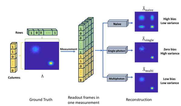
Figure 1: Schematic of the proposed reconstruction technique. A ground truth image is measured using the SNSPD array to give time-resolved row–column readouts. The readout rows and columns are used to reconstruct the ground truth image using three methods. The proposed multiphoton estimator provides the lowest mean-squared error among the techniques compared.

When more than one photon is incident on the array within a single integration period, the problem of resolving the spatial locations of incidence is ill-posed. As an example, consider the readout $R^{t}=[1,1]$ and $C^{t}=[1,1]$ from a $2\times 2$ array. This readout could have resulted from multiple detection events such as 2 photons at $\{(1,1)$,$(2,2)\}$, 2 photons at $\{(1,2)$, $(2,1)\}$, 3 photons at $\{(1,1$, $(1,2)$,$(2,1)\}$, and so on.

A naive reconstruction assumes that a photon was incident at each of the candidate pixels. This causes “ghost spots” in the reconstructed image as depicted in $\widehat{\Lambda}_{\rm naive}$ in Figure 1. A simple solution to prevent the ghost spots is to only use frames where a single row and a single column have fired for reconstruction, since these readouts are unambiguous with respect to the spatial location of photon incidence. However, this method disregards the information contained in frames with multiphoton coincidences. To utilize large-scale SNSPD arrays for imaging with a good count rate, there is a need to develop alternative reconstruction techniques that exploit the spatial dimensions of the array. The naive, single-photon, and our proposed mulitphoton reconstruction techniques depicted in Figure 1 are described in Section 3.

3 Estimators

In this section, we develop analytical expressions for three estimators: naive, single-photon, and multiphoton. For simplicity, we start with a $2\times 2$ array. The different types of photon incidences and their corresponding readouts in a $2\times 2$ array are shown in Figure 2. For the three estimators discussed in this section, the overall probability of detecting a photon at each pixel $(i,j)$ of the array can be denoted by $\widehat{Q}_{ij,\rm naive}$, $\widehat{Q}_{ij,\rm single}$, and $\widehat{Q}_{ij,\rm multi}$. The incident flux at each pixel can then be estimated elementwise as

$$\widehat{\Lambda}_{ij}=-\log\!\left(1-e^{-\widehat{Q}_{ij}}\right).$$ (4)

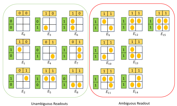
Figure 2: A $2\times 2$ array can have 16 possibilities for one or more detected photon. Row–column readout results in 9 unambiguous events $E_{0},E_{1},\ldots,E_{8}$ and 7 events $E_{9},E_{10},\ldots,E_{15}$ that are ambiguous because they all results in $R^{t}=[1,1]$ and $C^{t}=[1,1]$.

3.1 Naive Estimator

The naive estimator (NE) assumes that a photon is detected at each of the candidate pixels. Thus,

$$\widehat{Q}_{ij,\rm naive}=\frac{1}{T}\sum_{t=1}^{T}R_{i}^{t}C_{j}^{t}.$$ (5)

The naive estimator overestimates $q$, because it always counts ghost spots as photon detections. Let us compute the bias of $\widehat{Q}_{ij,\rm naive}$. For simplicity, we consider the case of $2\times 2$ array and assume that the probability of detecting more than two photons in a frame is negligible. Then, $R_{i}^{t}C_{j}^{t}=1$ if either of the following disjoint events occurs in frame $t$.

1. There is one photon detected at pixel $(i,j)$.

2. There are two photons detected – one in row $i$ and another in column $j$, but both photons are not at pixel $(i,j)$.

Then,

$$R_{i}^{t}C_{j}^{t}\sim\text{Bernoulli}\left(q_{ij}+q_{i,1-j}q_{1-i,j}\right).$$ (6)

Therefore, the bias of the naive estimator is

$$\mathbb{E}\left[{\widehat{Q}_{ij,\rm naive}}\right]-q_{ij}=q_{i,1-j}q_{1-i,j}.$$ (7)

3.2 Single-Photon Estimator

Since the naive estimator is biased and produces ghost spots in the reconstruction, we develop alternate methods to mitigate these artifacts. A simple way of preventing misattributions is to only use frames with a single detected photon in the reconstruction since these give the exact spatial locations of photon incidence. We consider the single-photon estimator (SPE):

$$\widehat{Q}_{ij,\rm single}=\begin{cases}\frac{N_{n(i-1)+j}}{N_{n(i-1)+j}+N_{0}},&\text{ if }N_{n(i-1)+j}+N_{0}>0;\\ 0,&\text{ if }N_{n(i-1)+j}+N_{0}=0,\end{cases}$$ (8)

where $N_{n(i-1)+j}$ is the number of frames where a photon is detected only at pixel $(i,j)$, and $N_{0}$ is the number of frames without any detected photons. Since we consider incident flux levels of a few photons per frame in this work, we assume that the probability of $N_{n(i-1)+j}+N_{0}=0$ is neglible; if all frames have more than 1 detected photon, setting the estimate $\widehat{Q}_{ij,\rm single}$ to 0 is arbitrary. Under these conditions, the SPE has approximately zero bias. To compute the bias, note that $N_{n(i-1)+j}$ and $N_{0}$ are the outcomes of a multinomial distribution. For a $2\times 2$ array,

$$(N_{0},N_{1},\ldots,N_{9})\sim\text{Multinomial}(r_{0},r_{1},...,r_{9};T),$$ (9)

where $N_{0},N_{1},\ldots,N_{8}$ are the numbers of frames for events $E_{0},E_{1},\ldots,E_{8}$ respectively, and $N_{9}$ is the number of all events $E_{9},\ldots,E_{15}$, as shown in Figure 2. The corresponding probabilities of their occurence is $r_{0},r_{1},...,r_{9}$. Consider the pixel $(1,1)$. The $\mathbb{E}[q_{11}]$ is the same as the conditional expectation, $\mathbb{E}\bigg{[}\frac{N_{1}}{N_{1}+N_{0}}\big{|}N_{1}+N_{0}>0\bigg{]}$, (since $P(N_{n(i-1)+j}+N_{0}=0)=0$) and can be obtained using the Taylor series expansion similar to [19]. Let $f(N_{1},N_{0})=N_{1}/(N_{1}+N_{0})$. Then,

$$\begin{split}f(N_{1},N_{0})&\approx f(\mathbb{E}[N_{1}],\mathbb{E}[N_{0}])+(N_{1}-\mathbb{E}[N_{1}])\frac{\partial f}{\partial N_{1}}(\mathbb{E}[N_{1}],\mathbb{E}[N_{0}])\\ &\quad+(N_{0}-\mathbb{E}[N_{0}])\frac{\partial f}{\partial N_{0}}(\mathbb{E}[N_{1}],\mathbb{E}[N_{0}]).\end{split}$$ (10)

The expectation of approximated $f(N_{1},N_{0})$ is therefore

$$\begin{split}\mathbb{E}\left[\frac{N_{1}}{N_{1}+N_{0}}\right]&\approx\mathbb{E}\left[\frac{Tr_{1}}{Tr_{1}+Tr_{0}}\right]+\mathbb{E}\left[(N_{1}-Tr_{1})\frac{Tr_{0}}{(Tr_{1}+Tr_{0})^{2}}\right]\\ &\quad-\mathbb{E}\left[(N_{0}-Tr_{0})\frac{Tr_{1}}{(Tr_{1}+Tr_{0})^{2}}\right].\end{split}$$ (11)

Since $\mathbb{E}[N_{1}]=Tr_{1}$ and $\mathbb{E}[N_{0}]=Tr_{0}$, the expectation simplifies to

$$\mathbb{E}\left[\frac{N_{1}}{N_{1}+N_{0}}\right]\approx\frac{r_{1}}{r_{1}+r_{0}}.$$ (12)

Further, $r_{1}=q_{11}(1-q_{12})(1-q_{21})(1-q_{22})$ and $r_{0}=(1-q_{11})(1-q_{12})(1-q_{21})(1-q_{22})$, Equation 12 reduces to $\mathbb{E}\left[\frac{n_{11}}{n_{11}+n_{0}}\right]=q_{11}$. Therefore, the SPE is approximately unbiased.

3.3 Multiphoton Estimator

While the SPE provides a simple way to compute an approximately unbiased estimate, it discards frames with multiple detected photons and hence has a high variance. Here, we develop an analytical expression for the multiphoton estimator (ME) which utilizes photon counts from ambiguous readouts for reconstruction. We first consider the maximum-likelihood estimation method (MLE). The likelihood function of the readouts from all frames can be written as:

$$\mathcal{L}(q_{11},q_{12},...,q_{nn})=\left(\prod_{i=1}^{n}\prod_{j=1}^{n}(1-q_{ij})^{U_{ij}}(q_{ij})^{F_{ij}}\right)\left(\prod_{m\in N_{\rm amb}}(q_{m,\rm amb})^{m}\right)$$ (13)

where $U_{ij}$ and $F_{ij}$ are the number of unambiguous readouts where pixel $(i,j)$ has zero and at least one incident photons respectively, $N_{\rm amb}$ is the set containing the number of ambiguous readouts of each type and $q_{\rm amb}$ is the corresponding probability of each type of ambiguous readout.

For a $2\times 2$ array as shown in Figure 2, the only ambiguous readout type is $R^{t}=[1,1]$ and $C^{t}=[1,1]$. Each of the events $E_{9},\ldots,E_{14}$ can result in this readout. Thus, Equation 13 takes the form:

$$\mathcal{L}(q_{11},q_{12},q_{21},q_{22})=\left(\prod_{i=1}^{2}\prod_{j=1}^{2}(1-q_{ij})^{U_{ij}}(q_{i})^{F_{ij}}\right)(q_{11}q_{22}+q_{12}q_{21}-q_{11}q_{12}q_{21}q_{22})^{N_{9}}$$ (14)

where $N_{9}$ is the number of readouts such that $R^{t}=[1,1]$ and $C^{t}=[1,1]$, which are result from any of the events $E_{9},\ldots,E_{14}$. Thus, the probability of the union of events $E_{9},\ldots,E_{14}$ gives the last term in equation (14). As the log-likelihood is nonconcave due to this term, computing the maximum likelihood estimate is challenging. However, if we can estimate the probability of occurrence of each of the events $E_{9},\ldots,E_{14}$ individually, given that an ambiguous frame is measured, we can divide the last term into seven different terms. Let $g_{1}$,$g_{2}$,…,$g_{7}$ represent the conditional probabilities of the events $E_{9}$, $E_{10}$, …, $E_{15}$. An approximate likelihood function can now be written as:

$$\mathcal{L}(q_{11},q_{12},\ldots,q_{22})=\left(\prod_{i=2}^{n}\prod_{j=2}^{n}(1-q_{ij})^{U_{ij}+U_{ij}^{a}}(q_{ij})^{F_{ij}+F_{ij}^{a}}\right)$$ (15)

where $U_{ij}^{a}$ and $F_{ij}^{a}$ are the number of ambiguous readouts where pixel $(i,j)$ has zero and at least one incident photon respectively. We estimate $U_{ij}^{a}$,$F_{ij}^{a}$ as:

$$\centering U_{ij}^{a}=\sum_{g\in G_{ij}^{e}}gN_{9},\qquad F_{ij}^{a}=\sum_{g\in G_{ij}^{f}}gN_{9}\@add@centering$$ (16)

where $G_{ij}^{u}$ and $G_{ij}^{f}$ are sets containing the probabilities of each type of multiphoton event where pixel $(i,j)$ has no detected photons and at least one detected photon respectively conditioning on the event that the readout is ambiguous. Note that $\sum_{i=1}^{7}g_{i}$ = 1. As an example, consider pixel $(1,1)$ in Figure 2. $G_{11}^{f}$ contains the conditional probabilities of the events $E_{9}$, $E_{11}$, $E_{12}$, $E_{13}$, and $E_{15}$ while $G_{11}^{e}$ contains the conditional probabilities of events $E_{10}$ and $E_{14}$. To compute the conditional probability $g$ for each of these events, we leverage the single-photon estimate at each pixel. Let, $g_{1},\ldots,g_{7}$ represent the the conditional probabilities of events $E_{9},\ldots,E_{15}$. Let $E_{\rm amb}$ represent the event that an ambiguous readout is measured. In this case, $E_{\rm amb}=\bigcup_{i=9}^{15}E_{i}$. The conditional probability $g_{1}$ can now be calculated as follows:

$$g_{1}=P(E_{9}|E_{\rm amb})=\frac{P(E_{9})}{P(E_{\rm amb})}$$ (17)

Using the single-photon probability estimate at each pixel $\widehat{q}_{ij}^{s}$ in Equation 17, we get an estimate of $g_{1}$:

$$\widehat{g}_{1}=\frac{\widehat{q}_{11}^{s}\widehat{q}_{22}^{s}(1-\widehat{q}_{12}^{s})(1-\widehat{q}_{21}^{s})}{\widehat{q}_{11}^{s}\widehat{q}_{22}^{s}+\widehat{q}_{12}^{s}\widehat{q}_{21}^{s}-\widehat{q}_{11}^{s}\widehat{q}_{12}^{s}\widehat{q}_{21}^{s}\widehat{q}_{22}^{s}}$$ (18)

Similar estimates can be derived for $g_{2},\ldots,g_{7}$. Finally, the multiphoton estimate of the probability of detecting a photon at pixel $(i,j)$ for a $2\times 2$ array can be written as:

$$\begin{split}\widehat{q}_{11}=\frac{N_{1}+N_{5}+N_{6}+N_{9}(g_{1}+g_{3}+g_{4}+g_{5}+g_{7})}{N},\\ \widehat{q}_{12}=\frac{N_{2}+N_{5}+N_{7}+N_{9}(g_{2}+g_{3}+g_{4}+g_{6}+g_{7})}{N},\\ \widehat{q}_{21}=\frac{N_{3}+N_{6}+N_{8}+N_{9}(g_{2}+g_{4}+g_{5}+g_{6}+g_{7})}{N},\\ \widehat{q}_{22}=\frac{N_{4}+N_{7}+N_{8}+N_{9}(g_{1}+g_{3}+g_{5}+g_{6}+g_{7})}{N}\end{split}$$ (19)

Computing the bias of the multiphoton estimates analytically is complex since the terms $g_{1},\ldots,g_{7}$ are random. Numerical simulations show the ME has a low bias although it is not unbiased. Furthermore, the ME depends on the SPE for an estimate of the prior detection probability at each pixel. Thus, in cases where the SPE is poor (due to few single-photon frames), the mean-squared error of the ME reconstruction is high.

3.4 Scaling to Higher Dimensional Arrays

Although illustrated for a $2\times 2$ array, the multiphoton solution in Equation 19 can be used with higher dimensional arrays where 2 rows and 2 columns have photon incidences. However, in these cases, the total set of measurements includes ambiguous readouts of other types. For instance, in a $3\times 3$ array, we can have the following ambiguous readouts:

• 2 rows and 3 columns fired - 6 candidate pixel locations.

• 3 rows and 2 columns fired - 6 candidate pixel locations.

• 3 rows and 3 columns fired - 9 candidate pixel locations.

Using the approximate ML method described in the previous section to resolve these ambiguous readouts requires the modification of the term $q_{m,\rm amb}$ in Equation 13 and the expressions for conditional probabilities $g_{i}$’s to account for additional events. For instance, consider $R=[1,1,0]$ and $C=[1,1,1]$ in a 3x3 array. This readout can be the result of six different 3-photon events, twelve different 4-photon events, six different 5-photon events, or a 6-photon events. It is evident that as the number of rows and columns with photon coincidences increases, the number of unique terms in the expressions for $q_{m,amb}$ and $g_{i}$’s grows rapidly. As a result, we restrict our analysis and simulations to the 4-photon coincidence case and ignore terms resulting from 5-photon coincidences and above. This means that the readout $R=[1,1,0]$ and $C=[1,1,1]$ can only result from 3 or 4 photons being incident on the array, although 6 coincident photons would result in the same readout. Thus, our multiphoton estimator can resolve up to 4 photon coincidences at a minimum of 4 ambiguous pixel locations (2 rows and 2 columns case) and a maximum of 16 ambiguous pixel locations (4 rows and 4 columns case). We expect that the assumption of at most 4-photon coincidences introduces a small bias in the ME which is confirmed by numerical simulations.The results of reconstructing a ground truth image using NE, SPE, and ME are shown in the following section.

4 Results

4.1 Imaging Natural Scenes

Figure 3 shows the Monte Carlo simulation results of reconstructing a 32x32 ground truth image using each of the estimators. Each simulation consists of 100 trials, with 100,000 frames per trial. Reconstructions in rows (a),(b),(c), and (d) have an average of 3 photons per frame (PPF), while row (e) has a PPF of 4. In rows (a),(b), and (c), it can be seen that the NE introduces horizontal and vertical streaks due to misattributions from multiphoton coincidences. In row (a) the SPE achieves $\sim$5dB PSNR improvement over the NE and doesn’t show the same artifacts. However, we observe that the image is blurry and the petals of the flower appear noisy. Our proposed ME performs much better than both the SPE and NE. It outperforms the naive estimator by  6-10dB while its improvement over the single-photon estimator is  4-6dB. Further, we note that the ME preserves features in the ground truth image better than both the other estimators. The petals of the flower in row (a) are more clearly visible, while these are missing in the other reconstructions.

The improvement in the reconstruction depends on some features of the ground truth image. For example, in row (d) we consider a rotated version of the BU logo in row (b). It can be seen that the misattributions in the NE are more concentrated towards the center of the image as compared to row (b) where the horizontal and vertical streaks cut across the image. The PSNR of the naive reconstruction is lower than that in row (b), however, the multiphoton reconstruction achieves  5dB improvement compared to row (b). In row (e) we consider the BU logo with a PPF of 4. We note that the PSNR of the NE reduces by $\sim$ 0.4 dB while the PSNR of the SPE and ME reduce by $\sim$ 3 dB each. This behavior is expected as with an increase in the average PPF, the number of frames with a single detected photon decreases, which reduces the PSNR of the SPE and consequently the ME.

\begin{overpic}[width=390.25534pt,trim=42.67912pt 312.9803pt 28.45274pt 341.43306pt,clip]{fig/yellow_lilly.pdf} \put(-5.0,15.0){(a)} \put(5.0,28.0){Ground Truth} \put(35.0,28.0){Naive} \put(56.0,28.0){Single-Photon} \put(82.5,28.0){Multiphoton} \end{overpic}\begin{overpic}[width=390.25534pt,trim=42.67912pt 312.9803pt 28.45274pt 341.43306pt,clip]{fig/BULogo.pdf} \put(-5.0,15.0){(b)} \end{overpic}\begin{overpic}[width=390.25534pt,trim=42.67912pt 312.9803pt 28.45274pt 341.43306pt,clip]{fig/Coins.pdf} \put(-5.0,15.0){(c)} \end{overpic}\begin{overpic}[width=390.25534pt,trim=42.67912pt 312.9803pt 28.45274pt 341.43306pt,clip]{fig/BULogo-Rotated.pdf} \put(-5.0,15.0){(d)} \end{overpic}\begin{overpic}[width=390.25534pt,trim=42.67912pt 312.9803pt 28.45274pt 341.43306pt,clip]{fig/BULogo-PPF4.pdf} \put(-5.0,15.0){(e)} \end{overpic}

Figure 3: Comparison of the estimator performance on the reconstruction of natural images. Rows (a - c) show that the multiphoton estimator is between 4-6dB better than the single-photon estimator and around 6-10dB better than the naive estimator. Row (d) shows the impact of rotating the ground truth image on the reconstruction. Row (e) shows the impact of increasing the average number of coincident photons per frame from 3 to 4.

4.2 Optimal Photons Per Frame

To study the dependence of estimator performance on the incident photon flux, we perform a simulation with a high emitted photon flux from a source (PPF = 10) that is attenuated by a neutral density filter before being incident on the array. We then study the change in mean-squared error of the reconstructed image with an increase in the mean PPF. The results of this simulation are shown in Figure 4 (Right). Note that as the mean PPF increases, the MSE of all three estimators initially decreases, reaches a minimum, and then increases. While the increase in MSE at high PPF is expected, the high values at very low PPFs indicate that in this regime, attenuation $\alpha$ is the dominant contributor to the mean-squared error. It can also be seen that the minimum MSE of the multiphoton estimator is lower than that of the single-photon estimator and both of these are much lower than the naive estimator. Furthermore, the minimum value of MSE for the ME occurs at a PPF of 1.4 which is higher than that for the SPE at 0.9, and that for NE at 0.3. Thus, the ME produces a better reconstruction compared to both the NE and the SPE while operating at a higher incident photon flux.

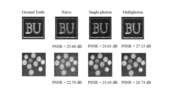
Figure 4: (Left) Reconstructions of images using the three estimators. (Right) Mean-squared errors of the estimators as a function of mean photons per frame.

Figure 4 (Left) shows a comparison of the estimators operated at their respective optimal attenuation values. The naive reconstruction in this case doesn’t possess the horizontal and vertical stripes in rows (a),(b) and (c) of Figure 3. This is because the incident photon flux has been sufficiently attenuated so that most readout frames contain only one photon. This is also reflected in the relatively small improvement observed by the SPE, compared to the same flux case as in Figure 3. While operating at their optimal attenuations, the single-photon estimator sees  1dB improvement over the naive estimator, while the multiphoton estimator achieves  4dB decrease in MSE over the naive estimator and  3dB decrease over the single-photon estimator respectively.

4.3 2,3 and 4-Photon Estimators

As explained in Section 3.4, our estimator resolves up to 4 simultaneously incident photons. The expression for $q_{m,\rm amb}$ in Equation 13 contains terms corresponding to conditional probabilities of every possible photon event that can result in the measured readout as shown in Equation 14.

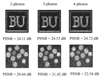
Figure 5: Increase in PSNR with increase in number of photons resolved by the multiphoton estimator. Mean PPF is kept constant at 3.

However, we can simplify this expression by restricting the number of events we consider as part of $q_{m,\rm amb}$. For instance, if we include only 2-photon coincidences in the case of a $2\times 2$ array, only conditional probabilities of events $E_{9}$ and $E_{10}$ would be summed in $q_{m,\rm amb}$. Here we compare the performance of the multiphoton estimator as the number of resolved photons increases from 2 to 4. Figure 5 shows the reconstruction of the BU logo and coins images with the 2,3 and 4-photon estimators. We observe a small increase in the PSNR ($\sim$0.2-0.4 dB) for the BU logo with each additional photon resolved whereas the increase is more signficant in the coins image ($\sim$0.8-1.1 dB). Note that the mean PPF for these reconstructions is constant at 3. This shows that when the incident photon flux is constant, reconstruction of the ME improves with an increase in the number of resolved photons.

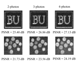
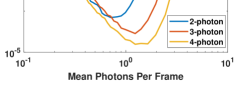
Figure 6: (Left) Reconstruction of BU logo and coins image using the 2-photon, 3-photon and 4-photon estimators at their optimal PPF values. (Right) MSE as a function of mean PPF for the three multiphoton estimators.

Figure 6 shows the behavior of the 2-photon,3-photon and 4-photon estimators as a function of the mean PPF. The 4-photon estimator has the lowest MSE that is attained at PPF = 1.4, whereas the 3-photon and 2-photon estimators achieve their lowest MSE at PPF = 1.23 and 0.7 respectively. In general, we note that as the term $q_{m,\rm amb}$ in Equation 13 includes more types of ambiguous readout events, the reconstruction quality improves both at constant incident flux and at different incident flux regimes.

\begin{overpic}[width=216.81pt,trim=28.45274pt 170.71652pt 49.79231pt 170.71652pt,clip]{fig/Final_ArraySize_1.pdf} \end{overpic}

\begin{overpic}[width=216.81pt,trim=28.45274pt 170.71652pt 49.79231pt 170.71652pt,clip]{fig/Final_ArraySize_2.pdf} \end{overpic}

Figure 7: (Left) Variation of the optimal PPF of the NE, SPE and ME with an increase in array size. (Right) Change in factor decrease of MSE for the three estimators with an increase in array size.

Since scaling SNSPD arrays to high spatial dimensions is an active area of research, here we study the behavior of the estimators as the array size increases from $2\times 2$ to $32\times 32$.

4.4 Scaling with Array Size

Figure 7 shows the change in performance of the NE, SPE and ME with an increase in the array size. It can be seen that the number of coincident photons per frame that results in optimal MSE is generally higher for the ME compared the SPE and the NE. Specifically, the optimal PPF value for the ME is greater than one across the range of array sizes. This indicates that the multiphoton estimator is well-suited for operation in flux regimes where more than one photon is incident on the array. Furthermore, we note that the factor decrease in MSE decreases with an increase in array size. However, for a $32\times 32$ array, our ME still achieves a decrease in MSE over the naive reconstruction by a factor of  5. With increasing array size, the number of unique ambiguous events also increases. Hence, this trend in part can be compensated by resolving more than 4-photon coincidences, although this can be computationally expensive.

5 Conclusions

In summary, we have demonstrated a new method to mitigate the artifacts introduced by the row-column readout architecture in state-of-the-art single-photon detector arrays. Our method, based on a combinatorial study of events that cause ambiguous readouts, achieves a significant improvement in image reconstruction over conventional techniques which either cause misattributions or discard ambiguous data. Since this reconstruction utilizes ambiguous readouts, it allows the utilization of the spatial dimensions of the array and consequently, operations at higher photon fluxes. Furthermore, our study provides a framework to resolve an abitrarily large number of multiphoton coincidences in larger arrays, although a brute-force implementation of such a solution would be computationally intractable. Nevertheless, our method shows that information contained in ambiguous readouts can be exploited to improve imaging capabilities of SNSPD arrays without requiring addittional hardware modifications. This could enable the wider use of SNSPD arrays in applications like lidar and quantum imaging.

References

- [1] Y. Guan, H. Li, L. Xue, et al., “Lidar with superconducting nanowire single-photon detectors: Recent advances and developments,” \JournalTitleOptics and Lasers in Engineering 156, 107102 (2022).
- [2] J. Rapp, J. Tachella, Y. Altmann, et al., “Advances in single-photon lidar for autonomous vehicles: Working principles, challenges, and recent advances,” \JournalTitleIEEE Signal Processing Magazine 37, 62–71 (2020).
- [3] T. Gerrits, S. Allman, D. J. Lum, et al., “A high-resolution single-photon camera based on superconducting single photon detector arrays and compressive sensing,” \JournalTitleProc. of IISW p. 300 (2015).
- [4] F. Villa, D. Bronzi, S. Bellisai, et al., “Spad imagers for remote sensing at the single-photon level,” in Electro-Optical Remote Sensing, Photonic Technologies, and Applications VI, vol. 8542 (SPIE, 2012), pp. 122–127.
- [5] L. You, “Superconducting nanowire single-photon detectors for quantum information,” \JournalTitleNanophotonics 9, 2673–2692 (2020).
- [6] M. Zarghami, L. Gasparini, L. Parmesan, et al., “A 32 32-pixel cmos imager for quantum optics with per-spad tdc, 19.48% fill-factor in a 44.64-m pitch reaching 1-mhz observation rate,” \JournalTitleIEEE Journal of Solid-State Circuits 55, 2819–2830 (2020).
- [7] I. Cusini, D. Berretta, E. Conca, et al., “Historical perspectives, state of art and research trends of spad arrays and their applications (part ii: Spad arrays),” \JournalTitleFrontiers in Physics 10, 906671 (2022).
- [8] C. Bruschini, H. Homulle, I. M. Antolovic, et al., “Single-photon avalanche diode imagers in biophotonics: review and outlook,” \JournalTitleLight: Science & Applications 8, 87 (2019).
- [9] F. Piron, D. Morrison, M. R. Yuce, and J.-M. Redouté, “A review of single-photon avalanche diode time-of-flight imaging sensor arrays,” \JournalTitleIEEE Sensors Journal 21, 12654–12666 (2020).
- [10] I. Holzman and Y. Ivry, “Superconducting nanowires for single-photon detection: progress, challenges, and opportunities,” \JournalTitleAdvanced Quantum Technologies 2, 1800058 (2019).
- [11] G. Luetzenburg, A. Kroon, and A. A. Bjørk, “Evaluation of the apple iphone 12 pro lidar for an application in geosciences,” \JournalTitleScientific reports 11, 22221 (2021).
- [12] M. Razali, A. Idris, M. Razali, and W. Syafuan, “Quality assessment of 3d point clouds on the different surface materials generated from iphone lidar sensor.” \JournalTitleInternational Journal of Geoinformatics 18 (2022).
- [13] S. Steinhauer, S. Gyger, and V. Zwiller, “Progress on large-scale superconducting nanowire single-photon detectors,” \JournalTitleApplied Physics Letters 118 (2021).
- [14] M. S. Allman, V. B. Verma, M. Stevens, et al., “A near-infrared 64-pixel superconducting nanowire single photon detector array with integrated multiplexed readout,” \JournalTitleApplied Physics Letters 106 (2015).
- [15] E. E. Wollman, V. B. Verma, A. E. Lita, et al., “Kilopixel array of superconducting nanowire single-photon detectors,” \JournalTitleOptics express 27, 35279–35289 (2019).
- [16] A. N. McCaughan, Y. Zhai, B. Korzh, et al., “The thermally coupled imager: A scalable readout architecture for superconducting nanowire single photon detectors,” \JournalTitleApplied Physics Letters 121 (2022).
- [17] B. G. Oripov, D. S. Rampini, J. Allmaras, et al., “A superconducting-nanowire single-photon camera with 400,000 pixels,” \JournalTitlearXiv preprint arXiv:2306.09473 (2023).
- [18] H. Wang, Z.-j. Li, X.-M. Hu, et al., “Image distortion by ambiguous multiple-photon detections in a superconducting nanowire single-photon imager and the correction method,” \JournalTitleOptics Express 31, 23579–23588 (2023).
- [19] F. Duris, J. Gazdarica, I. Gazdaricova, et al., “Mean and variance of ratios of proportions from categories of a multinomial distribution,” \JournalTitleJournal of Statistical Distributions and Applications 5, 1–20 (2018).