Detecting algorithmic bias in medical-AI models

Abstract

With the growing prevalence of machine learning and artificial intelligence-based medical decision support systems, it is equally important to ensure that these systems provide patient outcomes in a fair and equitable fashion. This paper presents an innovative framework for detecting areas of algorithmic bias in medical-AI decision support systems. Our approach efficiently identifies potential biases in medical-AI models, specifically in the context of sepsis prediction, by employing the Classification and Regression Trees (CART) algorithm. We verify our methodology by conducting a series of synthetic data experiments, showcasing its ability to estimate areas of bias in controlled settings precisely. The effectiveness of the concept is further validated by experiments using electronic medical records from Grady Memorial Hospital in Atlanta, Georgia. These tests demonstrate the practical implementation of our strategy in a clinical environment, where it can function as a vital instrument for guaranteeing fairness and equity in AI-based medical decisions.

1 Introduction

The integration of machine learning (ML) and artificial intelligence (AI) in healthcare has ushered in a new era of medical decision-making, characterized by advancements in precision diagnosis, personalized treatment, and enhanced patient care [19, 21]. These advancements, enabled by ML-based decision support systems, which we term medical-AI models, have the potential to transform the healthcare sector fundamentally; however, this rapid advancement in technology raises considerable ethical concerns, specifically concerning the inherent biases, both social and statistical, that may be encoded in the electronic health record (EHR) data that underpin these systems. The critical nature of healthcare decisions, coupled with the nuanced ethical landscape, underscores the urgency of identifying these biases to ensure fair and equitable ML applications in healthcare, especially for diverse and often underrepresented patient subpopulations.

Central to the discussion of ML in healthcare is the multifaceted challenges of clinical and algorithmic bias. From a clinical perspective, biases can be observed in two primary categories: explicit bias and implicit bias. Explicit biases refer to consciously held views and opinions of healthcare personnel, which directly result in differential treatment depending on particular characteristics of patients, such as race, ethnicity, or age [23, 1]. Conversely, implicit biases are subconscious prejudices that subtly but significantly influence clinical practices and decision-making, often avoiding straightforward identification and regulation [8, 11, 1, 10]. Although efforts have been made to eliminate explicit biases in the healthcare space, the impact of implicit biases on patient-provider interactions and outcomes remains prevalent[23]. These biases are of the utmost importance as they directly impact the data that serves as the foundation for ML models in the healthcare domain.

Algorithmic bias poses another significant challenge within the realm of ML and AI systems. This bias commonly emerges as a result of erroneous assumptions made during the training of prediction models, frequently mirroring biases present in the real world or originating from incorrect or insufficient datasets. Within the realm of healthcare, this bias has the potential to result in inaccurate diagnoses or suboptimal interventions, thereby disproportionately affecting particular subgroups of patients and further amplifying preexisting disparities. The exacerbation of existing disparities in healthcare data is well documented in terms of race [17, 20, 16], gender [15], and socio-economic status[9]. Recognition and mitigation of algorithmic bias remain of significant importance, especially in high-stakes situations where patients’ lives are at risk [10]. The complexity of identifying these biases arises from the sophisticated nature of algorithmic processes and the wide variety of potential biases that can arise from different data characteristics.

This study presents a novel application of a well-studied statistical approach, specifically the Classification and Regression Trees (CART) decision trees, to detect regions of algorithmic bias in medical AI models. This method offers a systematic and rigorous way to identify and quantify algorithmic bias, addressing the gaps in current methods that often assume known biases. Additionally, this method is model-agnostic, detecting bias regions by retrospectively analyzing the results of a given prediction algorithm. We implemented and evaluated this model using synthetic data simulations and a real-world healthcare dataset from Grady Memorial Hospital in Atlanta, Georgia. These case studies demonstrate our approach’s efficacy in identifying algorithmically biased regions and provide insights into the features that categorize these regions. This paper presents a novel approach to understanding and mitigating algorithmic bias in medical AI models, paving the way for safer and more trustworthy AI applications in this critical domain.

2 Related Works

With the growing integration of machine learning (ML) and artificial intelligence (AI) in medical models, there is also an increasing demand to identify and quantify the sources and types of algorithmic bias that exist in these systems. This section draws on the seminal works of Corbett-Davies et al.[6] and Xu et al.[24] to explore commonly used fairness definitions in the context of algorithmic bias, with a specific focus on measures for group fairness.

Demographic parity [6] evaluates the fairness of treatment between different protected groups, including those classified by race, sex, age, etc. This metric measures whether individuals in various categories achieve positive outcomes in proportion to their representation in the population. Demographic parity can be expressed mathematically as follows:

$$\text{P}(d(X)=1|Y=0,X_{p})=\text{P}(d(X)=1)$$

Here, $d(X)=1$ represents a positive outcome in the algorithm’s prediction, $Y=0$ represents the absence of a specific condition, and $X_{p}$ is a variable denoting membership in a protected group.

Anti-classification, also known as ”Fairness Through Unawareness”[14], prohibits the use of any protected features in the decision-making procedure of an algorithm. The objective is to proactively avoid any type of bias that may occur if these features were considered during the algorithm’s prediction process. Although direct, this method has drawbacks when non-protected features are strongly correlated with protected features. In such cases, simply eliminating these attributes may not be sufficient to eliminate bias.

Disparate impact[7] measures the proportion of positive outcomes for one group to the proportion for another and is often applied in legal and regulatory contexts. This metric plays an important role in identifying unintentional discrimination by analyzing the proportionality of positive outcomes between various protected attributes.

In a given dataset $\mathcal{D}=(X,Y,C)$ where $X$ represents the protected attribute, $Y$ includes the remaining attributes, and $C$ is the binary class predicted by the algorithm to be predicted, disparate impact focuses on the comparisons of outcomes between different groups. It is commonly linked to the ”80% rule”, a principle used to detect notable disparities in treatments or outcomes. The rule is defined mathematically as follows: $D$ has disparate impact if

$$\frac{\text{P}(C=1|X=0)}{\text{P}(C=1|X=1)}\leq\tau=0.8$$

Here, $\text{P}(C=1|X=0)$ and $\text{P}(C=1|X=1)$ represent the conditional probabilities of obtaining a positive outcome (class ”1”) for the minority (X=0) and majority (X=1) protected groups, respectively. The threshold $\tau=0.8$ signifies that if the ratio of these probabilities falls below 80%, the system is considered to have a disparate impact, indicating a potential unintentional bias against the minority group.

Calibration, according to Corbett-Davies and Goel [6], is the process of checking whether risk scores, which are estimates of the likelihood of something happening, are the same for all protected groups. This implies that a properly calibrated model’s predicted probabilities accurately represent the actual probability distributions across various groups. In turn, the outcomes should be independent of any protected attributes, given the risk score. Mathematically, calibration can be defined as follows: Given risk scores $s(x)$ as predicted by the model, calibration conditions are met when

$$\text{P}(Y=1|s(X),X_{p})=\text{P}(Y=1|s(X))$$

The expression $\text{P}(Y=1|s(X),X_{p})$ denotes the conditional probability of the occurrence Y=1 given the risk score $s(X)$ for individuals who are part of a protected group $X_{p}$. Alternatively, $\text{P}(Y=1|s(X))$ represents the chance of the event happening for any individual who possesses an identical risk score, regardless of their affiliation to a particular group.

Equalized odds, as described by Hardt et al. [12], is a metric that permits the prediction $\hat{Y}$ to be influenced by protected characteristics, but only through the target variable $Y$, thus preventing the features from acting as proxies for the protected attributes. This concept differs from demographic parity and promotes the use of features that enable the direct prediction of $Y$.

Equal opportunity [12] is a more robust indicator of equalized probabilities, which assesses whether individuals in similar circumstances have an equal probability of achieving a favorable result. In practice, this involves ensuring that the model’s positive predictions are distributed evenly among various demographic groups. This implies that the model should not exhibit a bias towards any particular group when it comes to reliably recognizing true positives.

Pan et al. [18] propose a novel machine learning (ML) framework called the ”Fairness-Aware Causal Path Decomposition” framework. This model-agnostic framework places a strong emphasis on explaining and quantifying the various causal mechanisms that contribute to overall disparities in model outcomes. This approach breaks down the decision-making process of an ML model into distinct causal paths. Each path represents a specific process by which the input variables (features) influence the model’s predictions. By analyzing these paths, the framework identifies how different features and their interactions impact the fairness or bias of the model.

2.1 Fairness Measure Limitations

While the group fairness measures outlined above are widely used to identify potential algorithmic bias in ML models, they have limitations. According to research by Castelnovo et al., [3], simply excluding protected features from the decision-making process does not inherently guarantee demographic parity. Achieving demographic parity may involve using different treatment strategies for different groups in order to mitigate the impact of correlations between variables, a strategy that may be considered inequitable or counterintuitive.

Kleinberg et al.[13] discuss the inherent challenges in satisfying both calibration and balance measures, such as those proposed by equalized odds and equal opportunity. The incompatibility of these measures underscores the complexity of achieving fairness in algorithmic systems, particularly when multiple fairness criteria are considered simultaneously.

AI-medical decision support systems frequently function as black-box models, oftentimes providing limited insight into the structure of their training data, if any, as well as no visibility into the parameters used in model development. Developing effective and fair prediction models in this context poses unique difficulties, such as the potential absence of patient demographic representation in the training data and, in some instances, the complete absence of demographic information. Additional challenges may include the possibility of health conditions or measurement variables being used as proxies for demographic data. Additional challenges may arise due to the potential use of health conditions or measurement variables as proxies for demographic data. This occurrence can be linked to the increased prevalence of distinct conditions among specific demographic groups, potentially influenced by genetic, environmental, or socio-economic factors. On the other hand, models that do not incorporate all extensive information and health conditions of a patient may result in an oversimplified model.

2.2 Contribution

To address these issues, this study proposes an approach that identifies areas in a model where patient outcomes are suboptimal. This approach allows researchers and clinicians to evaluate the reliability of a prediction model, $\mathcal{A}$, for a patient, $p$, considering their individual characteristics, $X_{p}$. It helps to evaluate the effectiveness of the model in making accurate predictions for a specific patient and to assess whether the model should be applied to that type of patient.

3 Proposed Method

Given a pre-trained prediction algorithm $\mathcal{A}$, our objective is to identify a region $\mathcal{S}$ in the $p$-dimensional feature space where the algorithm exhibits suboptimal performance, which we refer to as the ”algorithmic bias” region. Here $p$ represents the number of features which can be categorical and/or continuous-valued.

We assume that the true region $\mathcal{S}$ is defined by a subset of key variables (features) $j\in S$. For real-valued features, this is represented as $X_{j}\in[L_{j},U_{j}]$, with some lower and upper bounds, and for categorical value features $X_{j}\in C_{j}$, $j\in S$. For example, $p=10$ and $S=\{1,3\}$,the algorithmic bias region might be defined by age $X_{1}\in[35,50]$, gender $X_{3}=\{Female\}$.

This formulation implies that the subset of variables in the set $S$ will be the most critical in causing bias, defining the algorithmic bias region $\mathcal{S}$. For instance, in our example, age and gender are the two most important features in defining the algorithmic bias region $\mathcal{S}$. Fig. 1 illustrates the idea, where the algorithmic bias region is a box in the feature space for $X\in\mathbb{R}^{p}$.

Figure 1: Illustration of the algorithmic bias region $\mathcal{S}$ in the feature space, where the algorithm $\mathcal{A}$ exhibits suboptimal performance.

Without knowing the true algorithmic bias region, $\mathcal{S}$, of the algorithm $\mathcal{A}$, as represented using blue dots in Fig. 1, we want to estimate it using test data. We can evaluate the performance of the algorithm on a collection of test samples $x_{i}\in\mathbb{R}^{p}$, $i=1,\ldots,n$. The response associated with each test sample is $y_{i}\in\mathbb{R}$. Based on this, we can evaluate the algorithm performance using residuals.

$$\epsilon_{i}=y_{i}-f(x_{i}),\quad i=1,\ldots,n.$$

We note that alternative measures of algorithm performance, such as conformity scores, may replace residuals.

Our goal is to estimate the region $\widehat{\mathcal{S}}$ using $\{\epsilon_{i}\}_{i=1}^{n}$ as follows:

$$\widehat{\mathcal{S}}=\{X_{j}\in[L_{j},U_{j}]\mbox{ or }X_{j}\in C_{j},j\in\widehat{S}\},$$ (1)

where $S$, $L_{j}$, $U_{j}$, and $C_{j}$ are parameters to be determined.

Continuing with our previous example, if we estimate $\widehat{S}=\{1,5\}$, this implies that we have correctly predicted the first important feature and incorrectly predicted the second. If $\widehat{S}=S$, then we estimate the correct subset variables used to define the algorithmic bias region. Once $S$ is estimated, the other parameters can be easier to decide.

We hypothesize that the residuals within the bias region are larger. Thus, we formulate our problem as follows.

$$\begin{split}\max_{\widehat{S}}\frac{1}{n(\widehat{S})}\sum_{x_{i}\in\widehat{S}}|\epsilon_{i}|\end{split}$$ (2)

where $\widehat{S}$ is defined in (1), and $n(\widehat{S})$ represents the number of data points $\widehat{S}$.

We apply CART: Classification And Regression Trees, as proposed by Brieman et al. [2], to solve (2) with a regularization term accounting for tree complexity. CART partitions the feature space and provides a piecewise-constant approximation of the response function, here representing algorithm performance. The effectiveness of our methodology relies on the closeness of the estimated value $\widehat{S}$ to the true value $S$. This distance measure will be assessed using test samples $(x_{i},y_{i})$, taking into account the inherent stochastic nature of the data.

3.1 Classification and Regression Trees (CART)

The Classification And Regression Trees (CART) model, as proposed by Breiman et al.[2], is a non-parametric machine learning technique that is well suited for the prediction of dependent variables through the utilization of both categorical and continuous predictors. CART models offer a versatile approach to defining the conditional distribution of a response variable $y$ based on a set of predictor values $x$ [5]. The main idea behind the CART algorithm is to recursively partition the dataset (feature space) into subsets, with the aim of achieving progressively more homogeneous distributions of the response variable $y$ within each subset. These partitions are made recursively in a top-down fashion using a greedy approach. Beginning from the root node, an optimal feature and split point are identified based on an appropriate optimization metric. The feature, split-point pair defines the partition splitting the feature space, and this procedure is repeated for every sub-feature space that is created. These partitions will ultimately result in the binary tree structure consisting of interconnected root, decision, and terminal nodes as depicted in Figure 2.

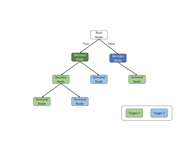
Figure 2: Typical CART structure

Root nodes encapsulate the entire dataset, forming the foundational layer. Decision nodes are points in the dataset characterized by features and split points that serve as points of division for partitioning the feature space. Each of these decision nodes extends branches to subsequent child nodes. Terminal (leaf) nodes are the final nodes in the tree, classifying or predicting data points based on their localized patterns.

CART models may be used for both classification and regression problems, as the name implies. Partitions are determined by using a specified loss function to evaluate the quality of a potential split and are based on both the features and feature values, that provide optimal splits. CART models, as applied to both tasks, have two main stages: the decision tree’s generation and subsequent pruning. We transition to a more granular discussion on CART’s implementation for both classification and regression problems.

Classification Trees

The CART method is used within the classification paradigm to make predictions about qualitative responses, specifically class labels, at terminal nodes. The objective is to maximize the Information Gain at each partition, hence maximizing the uniformity of the response variable in each node during the partitioning process. In the domain of decision trees, Information Gain gauges the value of the insight a feature offers about the target variable. In practical applications, this measure is determined using Entropy or the Gini index.

Entropy functions as a metric of disorder or unpredictability. It measures the impurity or randomness of a node, especially in binary classification problems. Mathematically, it is expressed as:

$$E=-\sum_{i=1}^{c}p_{i}\log_{2}p_{i}$$

where $p_{i}$ is the probability of an instance belonging to the $i^{th}$ class.

Gini Index serves as an alternate measure of node impurity. Considered a computationally efficient alternative to entropy, it is formulated as follows:

$$E=\sum_{i=1}^{c}p_{i}(1-p_{i})$$

where, yet again, $p_{i}$ is the probability of an instance belonging to the $i^{th}$ class.

Information Gain is a metric calculated by observing the impurity of a node before and after a split and is formulated as:

$$\text{IG}=E_{\text{parent}}-\sum_{i=1}^{c}w_{i}E_{\text{child}_{i}}$$

where $w_{i}$ is the relative weight of the child node with respect to the parent node.

Regression Trees

In contrast to their classification counterpart, regression trees exhibit notable performance in the prediction of continuous output variables. The key aspect of this problem involves partitioning the feature space to minimize the variation of the target variable inside each node. The variance, for a node with data points $y_{1},y_{2},\ldots,y_{N}$, is defined as:

$$V(D)=\frac{1}{N}\sum_{i=1}^{N}\left(y_{i}-\bar{y}\right)^{2}$$

where $\bar{y}$ represents the mean of the target variable for the data points in the node. The variance following a potential split is expressed by:

$$\Delta V=V(D_{\text{p}arent})-\sum_{i=1}^{N_{i}}w_{i}V(\text{D}_{child_{i}})$$

Tree Pruning

Without any constraints, the tree generation process of the CART algorithm will continue until each point is represented by a leaf node. Fully growing a tree to maturity will make the model vulnerable to overfitting. Tree pruning has been identified as a potential solution, which involves selective removal of branches from the tree to promote improved generalization. Implementing constraints such as minimal sample split, maximum tree depth, and cost-complexity pruning are employed to optimize the depth and fit of the decision tree. In particular, cost-complexity pruning, or weakest link pruning, is a technique that uses a parameter $\alpha$ to strike a balance between the depth of a decision tree and its fit to the training data. The trade-off is quantified by the following equation:

$$R_{\alpha}(T)=R(T)+\alpha|T|$$

Here, $R(T)$ is the misclassification rate of the tree $T$ and $|T|$ represents the count of the terminal nodes. The parameter $\alpha\geq 0$ controls the trade-off, with larger values of $\alpha$ resulting in smaller trees.

3.2 Algorithmic Bias Detection via CART

The CART algorithm is designed to iteratively partition the feature space. Its primary objective is to maximize the homogeneity within each resulting subset. In the regression setting, this is achieved by minimizing the variance of the data points within each subset. The algorithm’s design enables the isolation of similar data points into distinct leaf nodes.

Consider a regression tree, denoted as $\mathcal{T}$. Within this tree, each node $m$ represents a specific region $R_{m}$ in the feature space, encompassing $N_{m}$ observations. For each observation $i$ in this region, the associated response variable is given by $y_{i}$. The algorithm’s goal is to recursively partition $R_{m}$ into two subregions, $R_{1}$ and $R_{2}$, in a manner that minimizes the sum of squared deviations from the mean response within each subregion. Mathematically, this objective is expressed as follows:

$$\min\left(\sum_{y_{i}\in R_{1}}(y_{i}-\hat{y}_{1})^{2}+\sum_{y_{i}\in R_{2}}(y_{i}-\hat{y}_{2})^{2}\right)$$

The CART algorithm excels in detecting and separating groups of data points in the response variable $y$ that display unique patterns or relationships with specific features. Given that there is a cluster of points in $y$ with reduced values, the CART algorithm will strategically make feature splits that effectively separate these clusters as effectively as possible. This process creates subgroups within leaf nodes where the response variable $y$ is mostly made up of points with similar values.

4 Experiments

In this section, we conduct experiments utilizing two synthetic data simulations and an extensive real-world healthcare dataset obtained from Grady Memorial Hospital in Atlanta, Georgia. The objective of the simulation studies is to methodically assess the effectiveness of the CART algorithm in the context of detecting algorithmic bias regions. This comparison is carried out by evaluating the coverage ratio, which serves as our primary performance criterion. This metric has been designed to effectively analyze and encompass the potential presence of an algorithmic bias region that may emerge within the feature space.

4.1 Performance Metrics

We introduce a refined performance metric, namely the coverage ratio, designed to account for the presence of distinct region(s) characterized by algorithmic bias within the feature space.

Coverage Ratio in $n$-Dimensional Space

The Coverage Ratio in $n$-dimensional space is a metric that quantifies the relationship between the hypervolumes of the true and estimated regions compared to the overlapping hypervolume covered by both regions. When $n=2$ or $n=3$, the coverage ratio is comparable to measuring the ratio of overlap between the area or volume of two sets, respectively. This metric is extended to higher-dimensional spaces as follows:

Given a dataset $\mathcal{D}\subset\mathbb{R}^{n}$, consider two n-dimensional bounded regions defined by sets $\mathcal{S}$ (true region) and $\mathcal{\hat{S}}$ (estimated region).

Let $|S\cap\hat{S}|$ denote the hypervolume of overlap common to both regions. The coverage ratio, $\mathit{CVR}$, for $N$ regions in an $n$-dimensional space is defined as:

$$\mathit{CVR}=\frac{1}{2N}\sum_{i=1}^{N}\left(\frac{|S_{i}\cap\hat{S}_{i}|}{|S_{i}|}+\frac{|S_{i}\cap\hat{S}_{i}|}{|\hat{S}_{i}|}\right)$$ (3)

Here, $|S_{i}|$ and $|\hat{S}_{i}|$ represent the hypervolumes of the true and estimated regions, respectively, in the $n$-dimensional space. The Coverage Ratio provides a measure of how well the estimated region approximates the true region in higher-dimensional space.

4.2 Simulation

To investigate the impacts of algorithmic bias within a feature space, we generated synthetic datasets, using multidimensional uniform distributions. In this simulation, we perform a set of experiments using a single implicit bias region on a range of sample sizes, represented as $n_{s}$ = [500, 750, 1000, 2000, 3000, 6000, 8000] in a lower-dimensional setting, i.e. $p$ = [2,3], and $n_{S}$ = [5000, 7500, 10000, 20000, 30000, 60000, 80000] for higher-dimensional settings, i.e. $p=[4,5,\ldots,P]$. Features $x_{i}\in i=0,1,\ldots,P$ were selected from a uniform distribution within the restricted range of [-10, 10]. The corresponding $y$ values for these data points were produced similarly from a uniform distribution, spanning the range [0.8, 1.0]. To incorporate algorithmic bias regions with alternate output distribution, a central point, denoted $c_{i}$, was stochastically chosen within the feature space. Subsequently, the data points located within a specified radius around the given central point were modified to ensure that their corresponding output values, $y$, followed a uniform distribution limited to the interval [0.3, 0.6]. The region having reduced output values in the feature space is indicative of the region that may possess algorithmic biases.

Synthetic data experiments

The focus of our initial experiment was to explore the relationship between the topology of the data samples and the resulting performance of the CART model given a fixed predefined algorithmic bias region. For each sample size, $n_{s}$, we established a single algorithmic bias region, which was maintained consistently throughout each replication of the experiment as our benchmark (true regions). The emphasis here was on experimenting with the positional variability of data points with the random generation of new data points in each replication.

In the second experiment, our objective was to measure the influence exerted by the location of the algorithmic bias region on the performance of the CART model. This experiment maintained a fixed feature space topology across each replication, allowing the analysis to focus on the implications of varying the location of the algorithmic bias region.

The effectiveness of the model was evaluated using the coverage ratio performance metric as described above. This metric was used to compare the estimated region produced by the model with the previously defined true region.

4.3 Real Data Experiments

The real data experiment is divided into two main phases: first, we use extreme gradient boosting (XGBoost) to develop a time series-based sepsis prediction model on a diverse patient cohort; second, we use the predictions of the model to evaluate its performance measures and identify regions of algorithmic bias. This section begins with a discussion of how the data was selected and how a cohort definition for the sepsis prediction model was developed. Next, we explain how the data set was divided into training, validation, and test sets. Lastly, we explain the formulation of the XGBoost model and finish with a description of how we process the prediction model’s output using our algorithmic bias detection methodology.

4.3.1 Data

Electronic health record (EHR) data was retrospectively acquired from 16,167 adult subjects who were admitted to the intensive care unit (ICU) at Grady Memorial Hospital, Atlanta, Georgia. Data spanned years 2014 to 2020 and included a total of 17,782 individual patient visits, which we refer to as ”encounters”. The dataset includes a diverse range of continuous physiological measurements, vital signs, laboratory results, and medical treatment information. Data also incorporated demographic information, including age, sex, race, zip code, and insurance status. The following data preprocessing procedures were designed to support two primary tasks: developing the sepsis prediction model and detecting algorithmic bias.

Preprocessing: Prediction Model

Preprocessing of continuous physiological measurement data began with addressing data sparsity. We excluded patients with fewer than 24 hours of continuous data after admission to the ICU. We then implemented a six-hour rolling imputation technique in which missing values were forward-filled using the aggregated median value for each patient and feature. Lastly, we implemented a sliding window function to generate six-hour rolling window calculations that include mean, median, minimum, maximum, and standard deviation for each continuous feature.

4.3.2 Sepsis Definition

We adopted the revised Sepsis-3 definition as proposed by Singer et al.[22], which defines sepsis as a life-threatening organ failure induced by a dysregulated host response to infection. This definition was used to identify patients who meet the criteria for sepsis and to determine the most probable time of sepsis onset. To prioritize the early detection of sepsis, we introduced a six-hour lag on the sepsis response variable. The general demographic and clinical characteristics of the analyzed cohort of patients are summarized in Table 1.

Table 1: Baseline characteristics of study patients grouped by cohort

Grouped by sepsis
Variable		Overall	Non-Sepsis	Sepsis	P-Value
n		13246	8490	4756
Age, median [Q1,Q3]		55.0 [39.0,66.0]	53.0 [36.0,64.0]	58.0 [45.0,68.0]	$<$0.001
Gender, n (%)	Female	4588 (34.6)	2904 (34.2)	1684 (35.4)	0.169
	Male	8658 (65.4)	5586 (65.8)	3072 (64.6)
Race, n (%)	American Indian and Alaskan Native	39 (0.3)	29 (0.3)	10 (0.2)	$<$0.001
	Asian	141 (1.1)	97 (1.1)	44 (0.9)
	Black or African American	9088 (68.6)	5623 (66.2)	3465 (72.9)
	Hispanic	583 (4.4)	387 (4.6)	196 (4.1)
	Multi-Racial	44 (0.3)	27 (0.3)	17 (0.4)
	Native Hawaiian and Other Pacific Islander	9 (0.1)	3 (0.0)	6 (0.1)
	Other	119 (0.9)	72 (0.8)	47 (1.0)
	Unknown	163 (1.2)	102 (1.2)	61 (1.3)
	White or Caucasian	3060 (23.1)	2150 (25.3)	910 (19.1)
Length of stay (LOS): ICU, mean (SD)		7.1 (9.6)	4.3 (3.5)	12.2 (14.0)	$<$0.001
No. days on ventilator, mean (SD)		3.8 (9.7)	1.0 (2.6)	8.9 (14.4)	$<$0.001
LOS: hospital, mean (SD)		15.5 (21.2)	10.6 (10.6)	24.3 (30.6)	$<$0.001
Albumin, mean (SD)		3.1 (0.6)	3.3 (0.5)	2.8 (0.5)	$<$0.001
Anion Gap, mean (SD)		9.1 (2.8)	8.7 (2.3)	9.8 (3.5)	$<$0.001
Mean Arterial Pressure (MAP), mean (SD)		91.7 (10.8)	93.0 (11.0)	89.3 (10.1)	$<$0.001
Bicarbonate (HCO3), mean (SD)		25.2 (3.5)	25.6 (3.0)	24.5 (4.2)	$<$0.001
Blood Urea Nitrogen, mean (SD)		21.2 (17.2)	16.8 (12.6)	29.1 (21.1)	$<$0.001
Calcium, mean (SD)		8.2 (0.7)	8.4 (0.6)	8.0 (0.7)	$<$0.001
Chloride, mean (SD)		104.9 (5.5)	104.0 (4.8)	106.5 (6.4)	$<$0.001
Creatinine, mean (SD)		1.5 (1.7)	1.2 (1.5)	1.9 (1.9)	$<$0.001
Weight (lbs), mean (SD)		183.9 (52.9)	182.8 (48.7)	185.9 (59.7)	0.003
Glasgow Comma Scale, mean (SD)		12.5 (3.4)	13.7 (2.6)	10.4 (3.6)	$<$0.001
Glucose, mean (SD)		132.3 (37.4)	127.6 (35.1)	140.8 (39.9)	$<$0.001
Hematocrit, mean (SD)		32.8 (6.4)	34.0 (6.4)	30.8 (5.8)	$<$0.001
Hemoglobin, mean (SD)		11.0 (2.1)	11.4 (2.1)	10.4 (1.9)	$<$0.001
Platelets, mean (SD)		199.7 (87.3)	208.3 (83.1)	184.2 (92.3)	$<$0.001
Potassium, mean (SD)		4.0 (0.4)	4.0 (0.3)	4.0 (0.4)	$<$0.001
procedure, mean (SD)		0.0 (0.0)	0.0 (0.0)	0.0 (0.0)	$<$0.001
Heart Rate, mean (SD)		86.5 (14.9)	84.8 (14.9)	89.7 (14.5)	$<$0.001
Sodium, mean (SD)		139.1 (4.6)	138.3 (3.9)	140.7 (5.3)	$<$0.001
SpO2, mean (SD)		97.3 (1.9)	97.3 (1.7)	97.4 (2.2)	0.044
Respiratory Rate, mean (SD)		18.7 (2.8)	18.3 (2.5)	19.5 (3.2)	$<$0.001
White Blood Cell Count, mean (SD)		10.6 (5.2)	9.9 (4.2)	11.8 (6.6)	$<$0.001
Temperature, mean (SD)		98.5 (1.0)	98.4 (0.8)	98.7 (1.2)	$<$0.001

4.3.3 Train-Validation-Test Splits

To ensure that the labels of the response variables (in this case, ”sepsis,” which showed whether a patient was retrospectively diagnosed with sepsis while in the ICU) are distributed proportionally between the training and test sets, we first performed a stratified training and test split of the original data. The stratified sampling process consisted of first calculating the proportion of each class in the original dataset. Next, we split the data into 80% training and 20% test sets. We then sampled data from the original data set so that the proportion of class labels in the training and test sets was comparable to that of the original dataset. This stratification was based on each individual patient encounter, with the aim of achieving proportional distributions of sepsis and non-sepsis encounters across both training and test sets compared to the original dataset. The training set consisted of 9,921 patient encounters, with 3,536 cases of sepsis and 6,385 cases of non-sepsis sequences. Similarly, the test set consisted of 2,493 patient encounters, with 880 cases of sepsis and 1,613 cases of non-sepsis sequences.

The training set was then put through five-fold stratified cross-validation to make the final training and validation sets. Each fold had an evenly split distribution of sepsis and non-sepsis patient encounters. We then implemented a sequential train-test split approach to partition each patient’s continuous physiological data. The first 24 hours of data for each patient were allocated for training, while the remaining data, up to the 168th hour, were used as a validation set to tune the model hyperparameters. The implementation of a 168-hour time limit was imposed to mitigate any potential impacts of data bias caused by potential complications that may affect a patient’s health status beyond the initial week of their ICU stay.

The test set was prepared following a similar protocol, using all continuous physiological data beginning with a patient’s admission to the ICU. Test set data was also subject to the same 168-hour limitation. We used this data to internally validate our model, with the test set consisting of completely new data sequences. The visual representation of the complete data preprocessing pipeline is depicted in Figure 3.

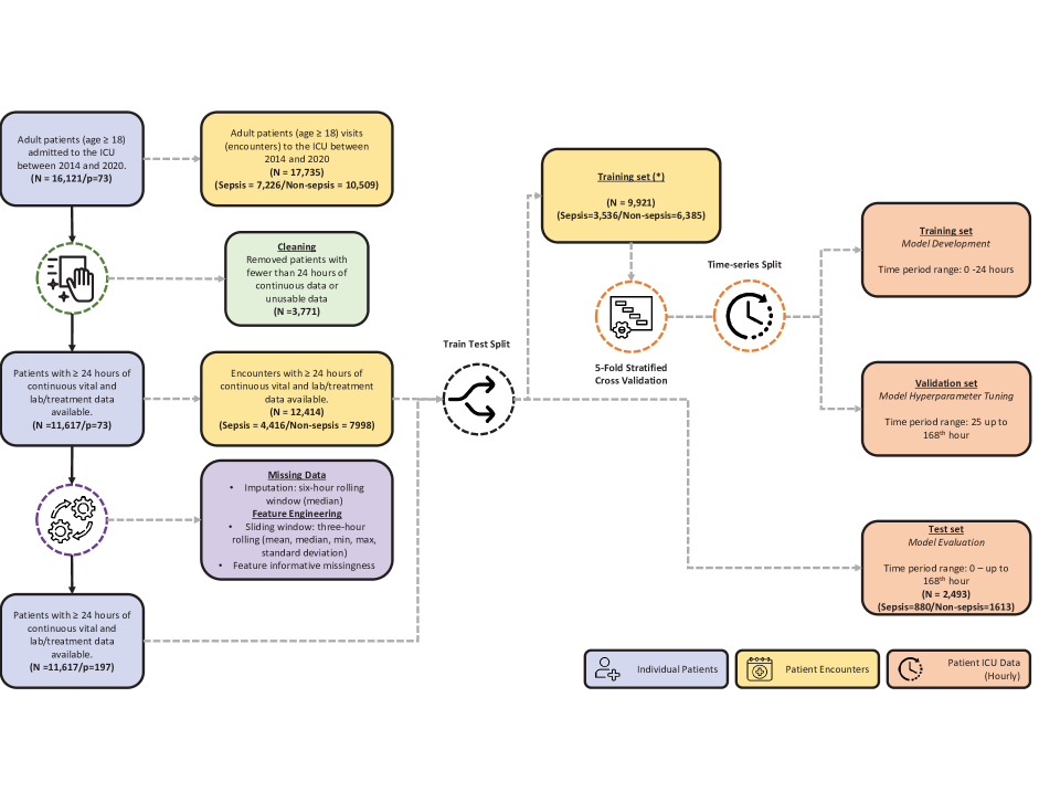
Figure 3: Data Preprocessing Diagram

4.3.4 Prediction Model

The foundation of the sepsis prediction model developed for this analysis was centered on the implementation of XGBoost [4], a robust tree-based gradient boosting algorithm known for its high computational efficiency and exceptional performance in managing complex and large datasets. We constructed this model using the Bayesian optimization technique with a Tree-structured Parzen Estimator (TPE) approach. We applied this method to optimize hyperparameters, which helped establish the learning process, complexity, and generalization capability of the model. Hyperparameters included but were not limited to, the following: max depth, learning rate, and alpha and lambda regularization terms.

The Bayesian optimization technique involved a series of 20 evaluations. In each iteration, we tune the hyperparameters with the aim of minimizing our selected loss function. For the purposes of sepsis prediction, we selected the f2-score as the loss function as it places more emphasis on the model’s recall performance. In the medical setting, the F2-score is particularly useful when the cost of false negatives (i.e., failing to accurately predict a patient having sepsis) is higher than that of false positives.

$$F2=5\left(\frac{{\rm precision}\times{\rm recall}}{4\times{\rm precision}+{\rm recall}}\right)$$

and we use the standard definition for precision and recall.

The final model is an ensemble based on the average five-fold cross-validation performance measured across the F2-score loss function.

4.3.5 Algorithmic Bias Detection

In the second stage of our real-data experiment, we assess the performance of the sepsis prediction model and identify potential algorithmic biases. We use the complete training dataset utilized for the development of the prediction model to perform this assessment. Here, each patient in the training set undergoes a sequential processing of their continuous data through the prediction algorithm. The subsequent calculation of each patient’s f2-score compares the algorithm’s sequential predictions with the actual observations made for that patient.

The f2-scores serve as the response variable for our algorithmic bias detection method. This process involves integrating the output of each patient’s visit from the prediction model with their respective demographic information. These demographic data include a variety of features such as sex, race, age, type of insurance, type and number of comorbidities, and reason for hospital admission.

Using this enriched dataset, we employ our algorithmic bias detection methodology, utilizing the CART (Classification and Regression Trees) algorithm. This enables the identification of potential areas in the feature space that may be subject to algorithmic bias. Figure 4 visually depicts the full bias detection process, providing an illustrative overview of how data flows through the analysis and how bias detection is integrated into this workflow.

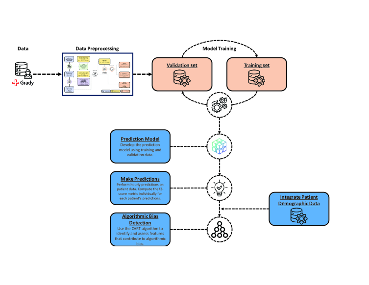
Figure 4: Algorithmic bias detection pipeline

5 Results

5.1 Simulation results

The simulation aimed to investigate the complex relationships between algorithmic bias regions and feature space topologies. Using a systematic and rigorous methodology, the experiments sought to gain insight into how these relationships affect the performance and reliability of the CART model. Figure 5 provides a visual representation of the ability of our approach to accurately estimate the borders of regions characterized by algorithmic bias. The true region(s) are delineated and filled in blue, whereas the estimated region(s) consist of points located inside the red dashed lines. Figure 5a illustrates an example of the simulated output in the context of a two-dimensional scenario. Similarly, Figure 5b demonstrates the ability to identify algorithmic biases in a three-dimensional scenario.

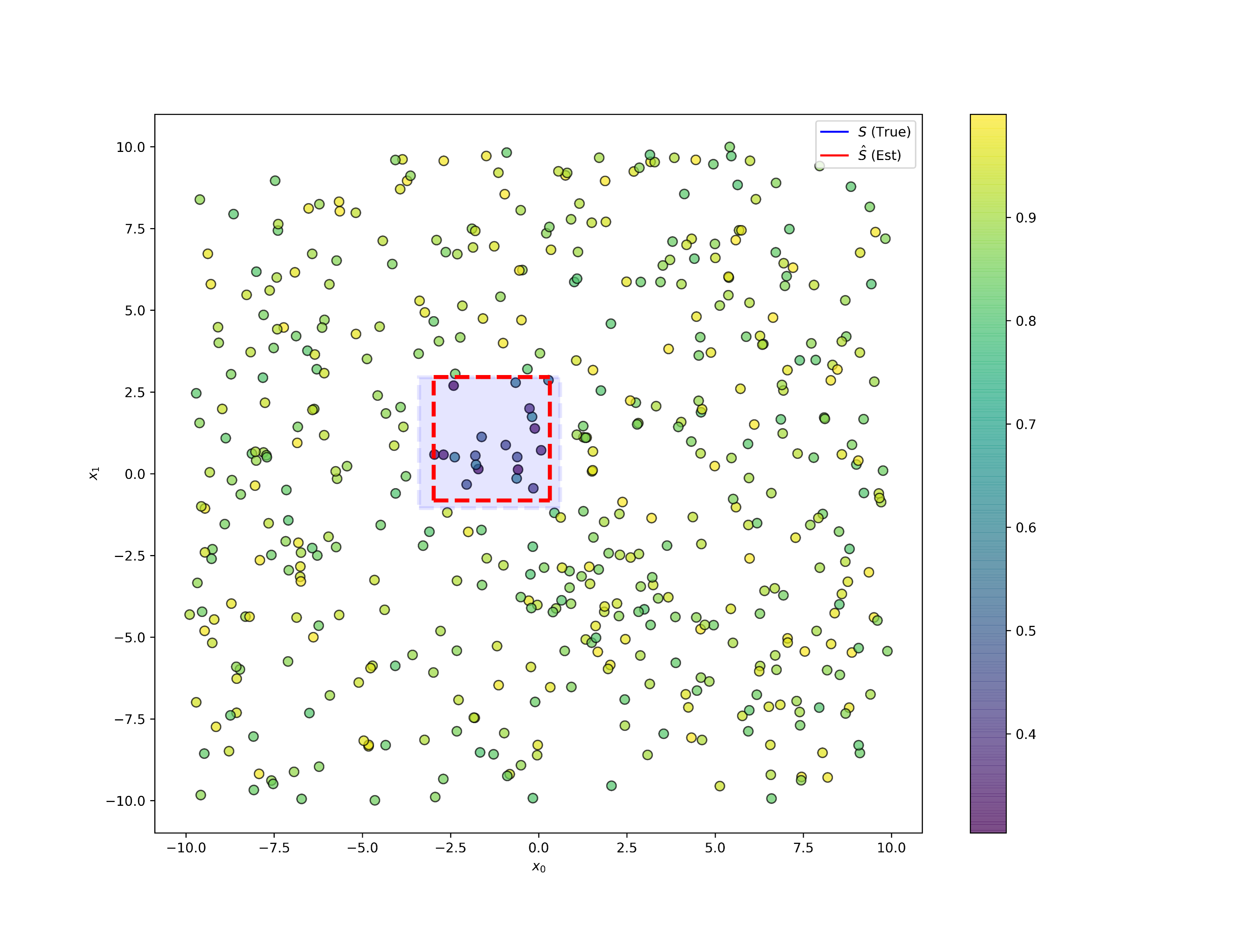
(a)

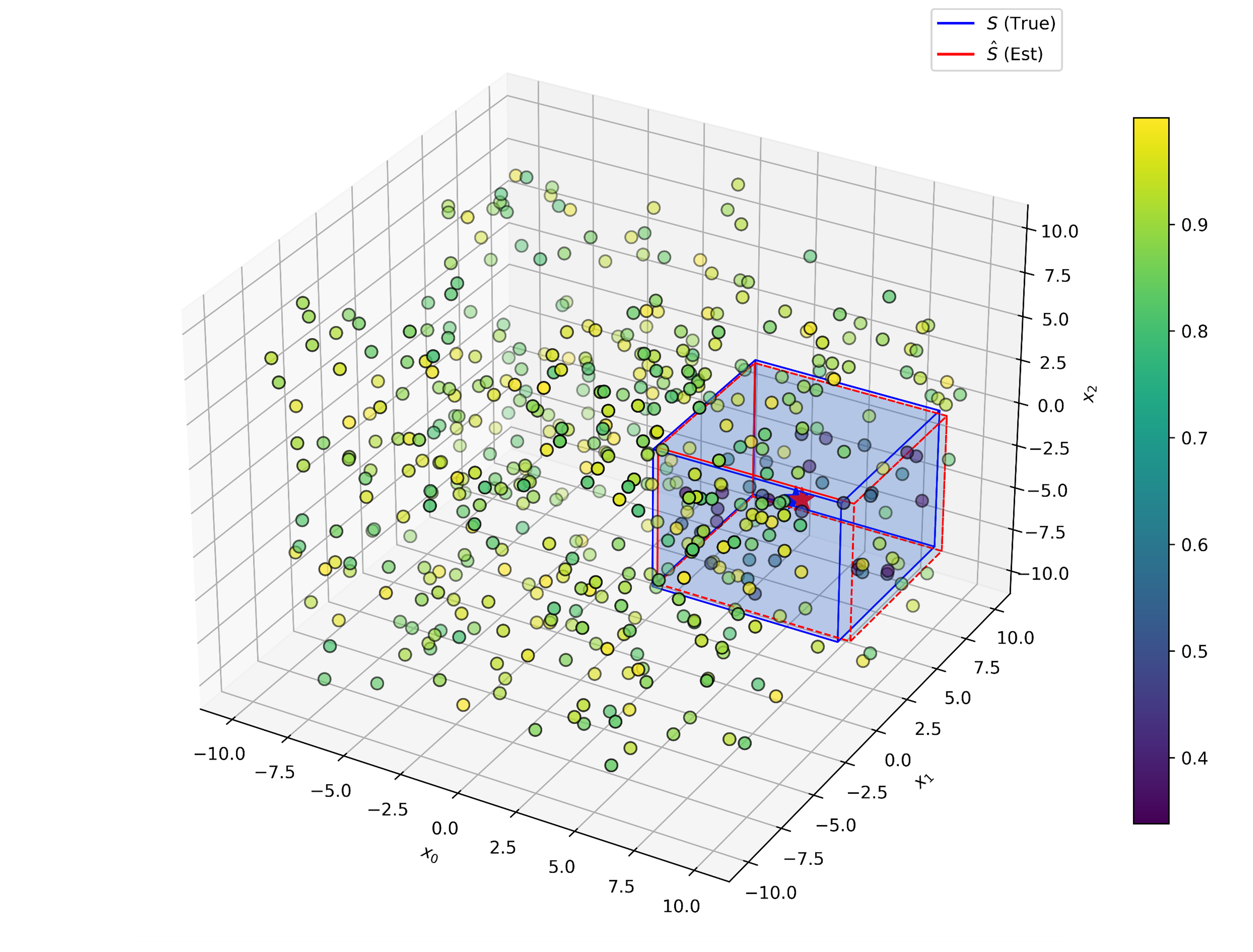
(b)

Figure 5: Examples of the experimental results in 2(a) and 3(b) dimensional space.

We provide a summary of the results achieved by our approach, as depicted in Figure 6, and confirm the efficacy of the CART algorithm in accurately detecting algorithmic bias regions. To provide precise details, Figure 6 shows the mean performance of each experiment at the various sample size test points for multiple $n$-dimensional cases. The figures incorporate 95% confidence intervals for both experiments. These results indicate that our method can efficiently detect the presence of algorithmic bias layered in the feature space.

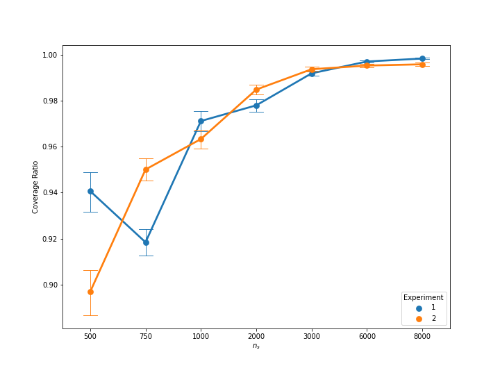
(a)

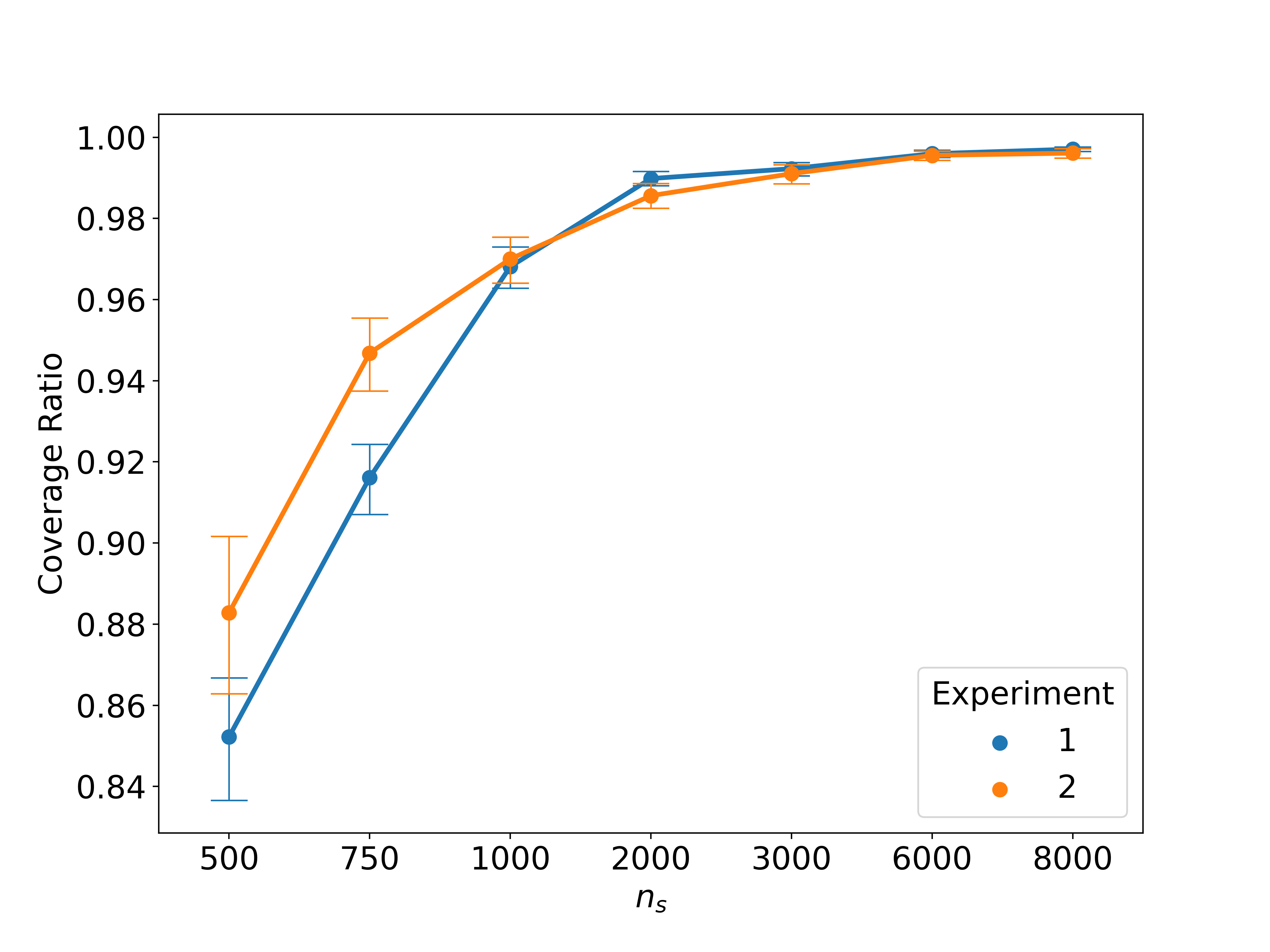
(b)

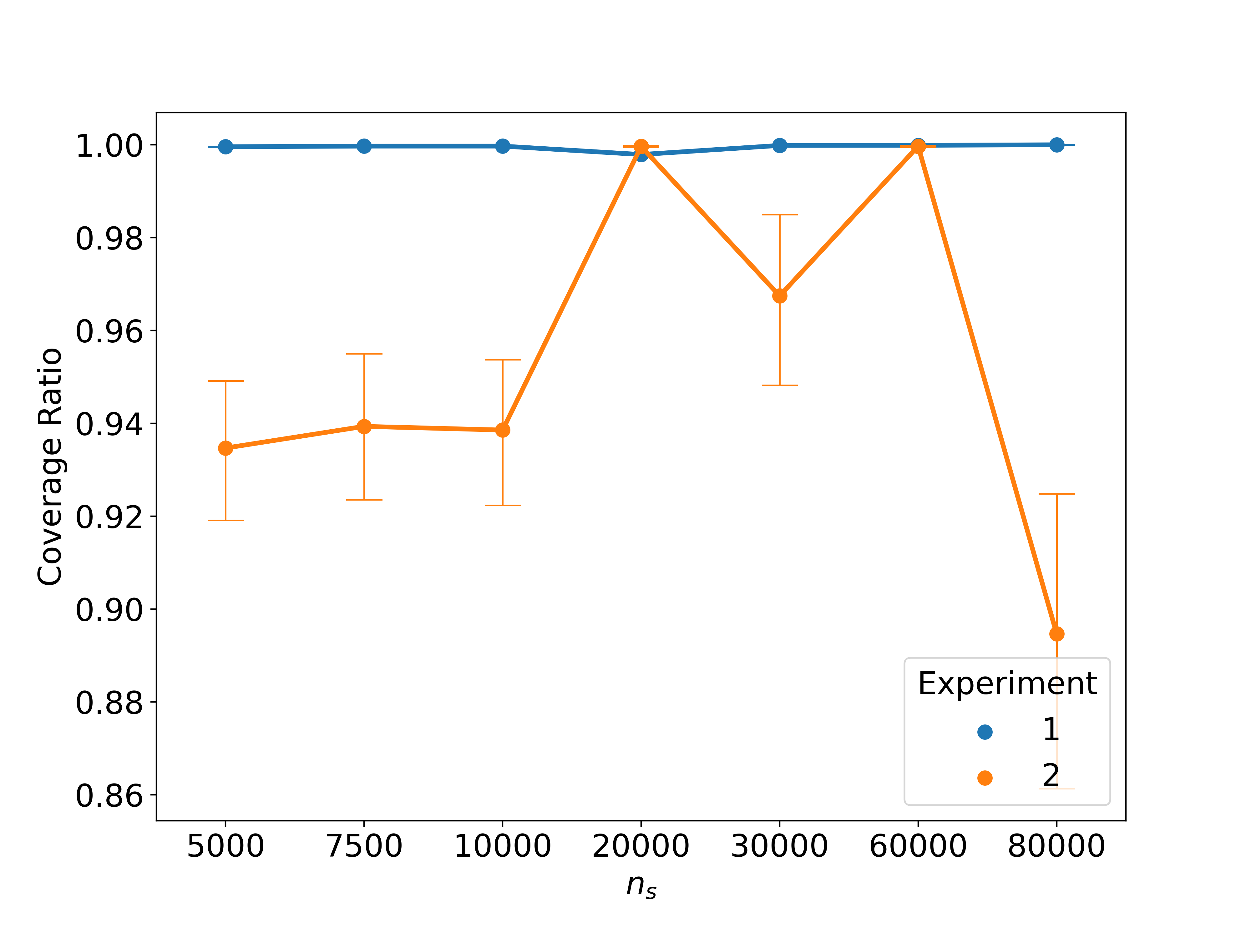
(c)

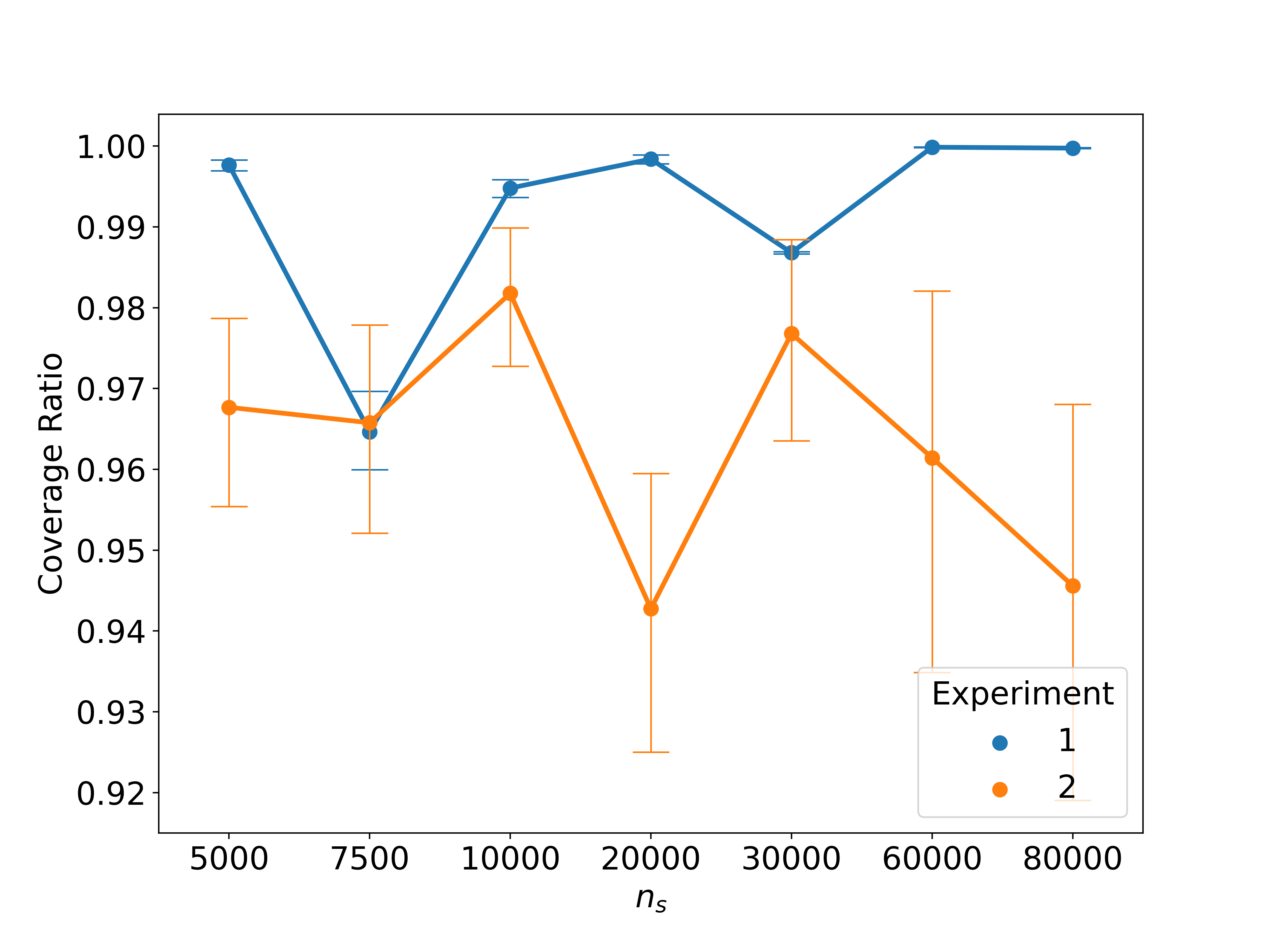
(d)

Figure 6: The plots show the mean coverage ratio for multiple $n$-dimensional test points: 2D(a), 3D(b), 4D(c), and 5D(d)

5.2 Real data experiment results

We summarize the complete performance of our sepsis prediction model in Figure 7. The results are organized according to the two previously described phases of the analysis, with each phase focused on different subsets of data. The first row of Figure 7 depicts the performance of the model based on the training set. Figure 7a illustrates the ability of the model to predict sepsis using a confusion matrix that presents the quantity (and proportion) of true positives, false positives, true negatives, and false negative results. Figure 7b presents the receiver operator characteristics (ROC) curve. The ROC curve is a graphical representation that shows the diagnostic ability of the prediction model by displaying the true positive rate (recall) versus the false positive rate (specificity) at different threshold values. The second row of the figure examines the model’s performance on the test data, providing insight into how well the model generalizes to unseen data. Similarly to the first row, Figure 7c illustrates the model’s predictive performance through a confusion matrix, while Figure 7d displays the ROC curve for the test data. Table 2 provides a detailed summary of the classification performance metrics of the prediction model.

(a)

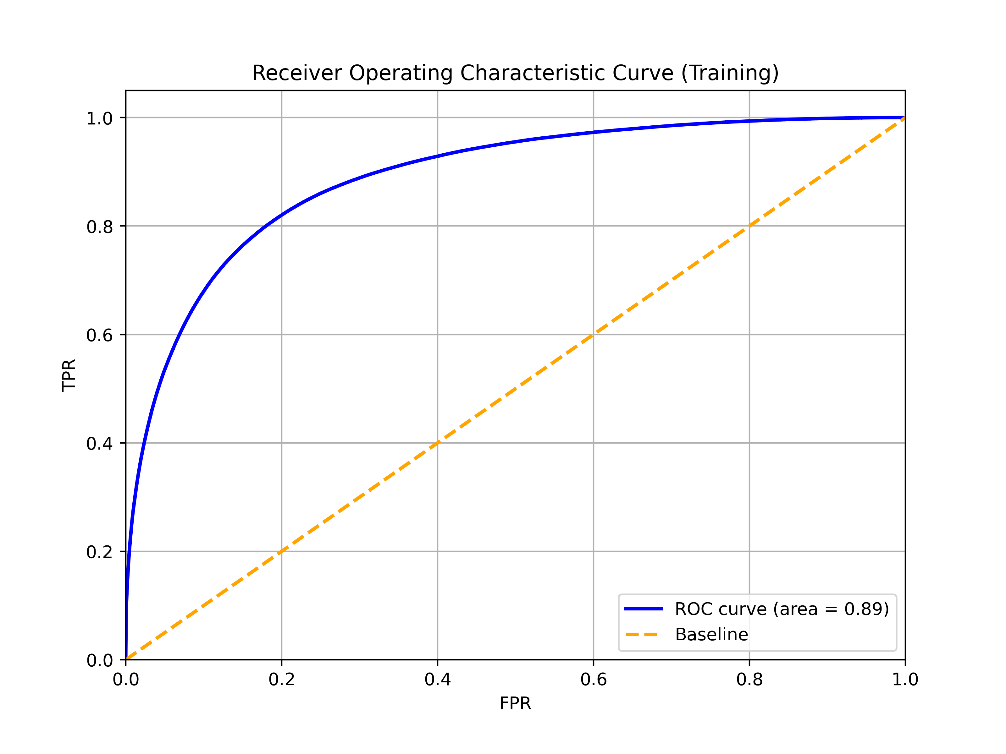
(b)

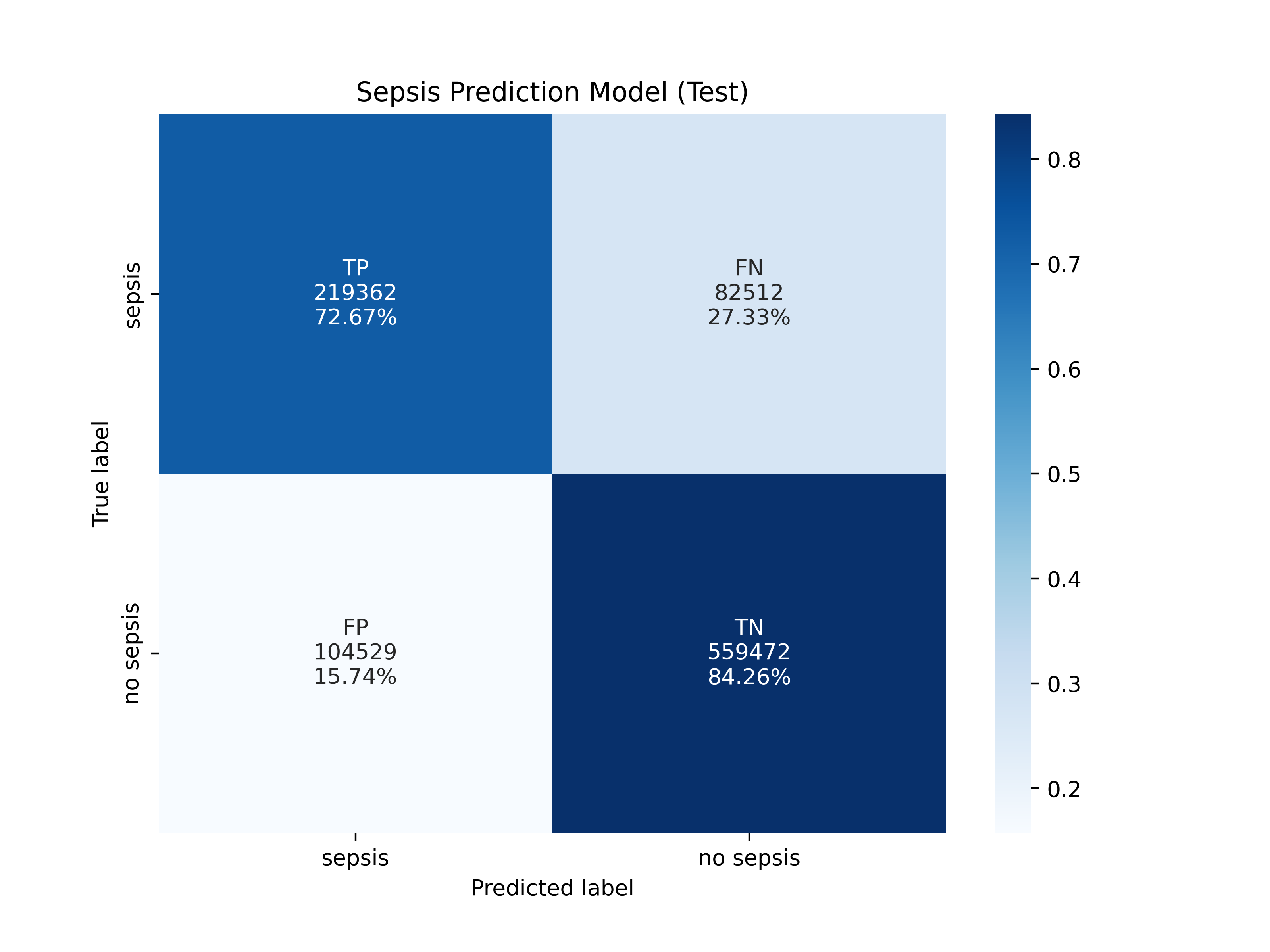
(c)

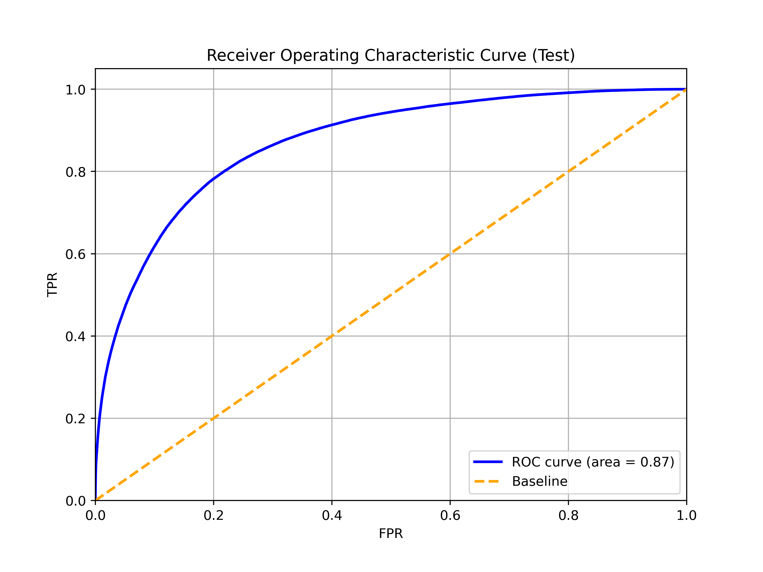
(d)

Figure 7: The plots present the sepsis prediction model’s performance measures. Plots (a) and (b) show the confusion matrix and ROC curve results of the model against the training data, respectively. Plots (c) and (d) provide similar measures for the test dataset.

	Accuracy	Precision	Recall	F1-Score	F2-Score
Training Set	0.82	072	0.75	0.74	0.75
Test Set	0.81	0.68	0.73	0.70	0.72

Table 2: Sepsis prediction model classification performance metrics for training and test sets

For the second stage of our real-data experiments, we used the f-s2-score as the primary measure of performance. After using the sepsis prediction model with the training data, we compute this measure for each patient. This metric represents how well the model predicts sepsis for each patient. We integrate this metric with each patient’s respective demographic information to produce a comprehensive dataset that offers an overview of the performance of the model in a diverse sample of patients. We use one-hot encoding to convert non-numeric features into a numeric representation. Additionally, we implement a five-fold cross-validated grid search technique to improve the performance of the CART algorithm. We do this to identify the best set of hyperparameters for the decision tree model. Figure 8 presents a graphical representation of the decision tree that was generated using the training data.

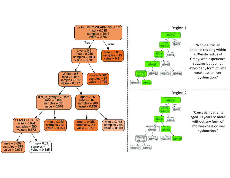
Figure 8: A visual representation of the decision tree derived from the training data. The right column highlights the two worst-performing regions with a summary of their respective paths.

The visualization’s left column displays the decision tree generated by the outcomes of the sepsis prediction model for the training data. The visualization’s right column highlights two nodes that demonstrate suboptimal performance. We identify these nodes as regions where potential algorithmic bias may be present within the model. In Region 1, the data points in the lowest node, which is colored green, are assigned a prediction value of 0.385. Region 2, which represents a different node, predicts a value of 0.609 for all data points within the node. To better characterize these regions, we mark the path from the root node to each poorly performing node of the decision tree. This path helps identify the specific circumstances that lead to these biased predictions. For example, in Region 1, the path from the root node to the worst-performing node can be represented by the path in Figure 9.

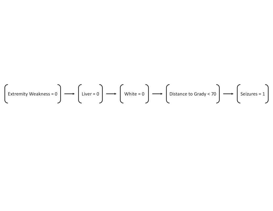
Figure 9: Illustration of the path from the root to suboptimal region

Based on this data, we can summarize this path as follows: ”Non-Caucasian patients living within a 70-mile distance from Grady, who have been hospitalized for seizures, but do not experience weakness in their limbs and do not have any liver disorders.” This summary offers a clear and practical explanation of the path of the decision tree, allowing a more comprehensive understanding of the demographic and clinical characteristics of the patient(s) linked to these biased areas.

Tracing decision tree routes and evaluating them in this way offers useful information about the decision-making process of the model. It emphasizes the key variables that have the greatest impact on the model’s predictions, enabling us to identify and potentially mitigate any potential biases in the model’s sepsis prediction approach.

6 Conclusion

This paper presents a new approach to detect and analyze regions of algorithmic bias in medical-AI decision support systems. This framework, which uses the Classification and Regression Trees (CART) method, is an important step in recognizing and dealing with potential biases in AI applications in the healthcare sector. We evaluated our technique through synthetic data experiments and successfully demonstrated the method’s ability to identify areas of bias, assuming that such regions exist in the data. Additionally, we extended our examination to a real-world dataset by carrying out an experiment using electronic health record (EHR) data obtained from Grady Memorial Hospital.

The increasing integration of machine learning and artificial intelligence in healthcare highlights the pressing requirement for tools, techniques, and procedures that guarantee the fair and equitable use of these technologies. The framework we present provides a tangible solution to this challenge. It offers a means for healthcare practitioners and AI developers to identify and remedy algorithmic biases, therefore promoting the development of medical ML/AI decision support systems that are both ethically sound and clinically effective.

References

- [1] Irene V Blair, John F Steiner and Edward P Havranek “Unconscious (Implicit) Bias and Health Disparities: Where Do We Go from Here?” In The Permanente Journal 15.2, 2011 DOI: 10.7812/tpp/11.979
- [2] Leo Breiman, Jerome H. Friedman, Richard A. Olshen and Charles J. Stone “Classification and regression trees” In Classification and Regression Trees, 2017 DOI: 10.1201/9781315139470
- [3] Alessandro Castelnovo et al. “A clarification of the nuances in the fairness metrics landscape” In Scientific Reports 12.1, 2022 DOI: 10.1038/s41598-022-07939-1
- [4] Tianqi Chen and Carlos Guestrin “XGBoost: A scalable tree boosting system” In Proceedings of the ACM SIGKDD International Conference on Knowledge Discovery and Data Mining 13-17-August-2016, 2016 DOI: 10.1145/2939672.2939785
- [5] Hugh A. Chipman, Edward I. George and Robert E. McCulloch “Bayesian CART model search” In Journal of the American Statistical Association 93.443, 1998 DOI: 10.1080/01621459.1998.10473750
- [6] Sam Corbett-Davies and Sharad Goel “The Measure and Mismeasure of Fairness: A Critical Review of Fair Machine Learning”, 2018
- [7] Michael Feldman et al. “Certifying and removing disparate impact” In Proceedings of the ACM SIGKDD International Conference on Knowledge Discovery and Data Mining 2015-August, 2015 DOI: 10.1145/2783258.2783311
- [8] Chloë Fitzgerald and Samia Hurst “Implicit bias in healthcare professionals: A systematic review” In BMC Medical Ethics 18.1, 2017 DOI: 10.1186/s12910-017-0179-8
- [9] Milena A. Gianfrancesco, Suzanne Tamang, Jinoos Yazdany and Gabriela Schmajuk “Potential Biases in Machine Learning Algorithms Using Electronic Health Record Data” In JAMA Internal Medicine 178.11, 2018 DOI: 10.1001/jamainternmed.2018.3763
- [10] Anthony G. Greenwald et al. “Implicit-Bias Remedies: Treating Discriminatory Bias as a Public-Health Problem” In Psychological Science in the Public Interest 23.1, 2022 DOI: 10.1177/15291006211070781
- [11] William J. Hall et al. “Implicit racial/ethnic bias among health care professionals and its influence on health care outcomes: A systematic review” In American Journal of Public Health 105.12, 2015 DOI: 10.2105/AJPH.2015.302903
- [12] Moritz Hardt, Eric Price and Nathan Srebro “Equality of opportunity in supervised learning” In Advances in Neural Information Processing Systems, 2016
- [13] Jon Kleinberg, Sendhil Mullainathan and Manish Raghavan “Inherent trade-offs in the fair determination of risk scores” In Leibniz International Proceedings in Informatics, LIPIcs 67, 2017 DOI: 10.4230/LIPIcs.ITCS.2017.43
- [14] Matt Kusner, Joshua Loftus, Chris Russell and Ricardo Silva “Counterfactual fairness” In Advances in Neural Information Processing Systems 2017-December, 2017
- [15] Agostina J. Larrazabal et al. “Gender imbalance in medical imaging datasets produces biased classifiers for computer-aided diagnosis” In Proceedings of the National Academy of Sciences of the United States of America 117.23, 2020 DOI: 10.1073/pnas.1919012117
- [16] Jeff Larson, Surya Mattu, Lauren Kirchner and Julia Angwin “How We Analyzed the COMPAS Recidivism Algorithm” In ProPublica, 2016
- [17] Ziad Obermeyer, Brian Powers, Christine Vogeli and Sendhil Mullainathan “Dissecting racial bias in an algorithm used to manage the health of populations” In Science 366.6464, 2019 DOI: 10.1126/science.aax2342
- [18] Weishen Pan et al. “Explaining Algorithmic Fairness through Fairness-Aware Causal Path Decomposition” In Proceedings of the ACM SIGKDD International Conference on Knowledge Discovery and Data Mining, 2021 DOI: 10.1145/3447548.3467258
- [19] Nirali M. Patel et al. “Enhancing Next-Generation Sequencing-Guided Cancer Care Through Cognitive Computing” In The Oncologist 23.2, 2018 DOI: 10.1634/theoncologist.2017-0170
- [20] Michael J. Pencina, Benjamin A. Goldstein and Ralph B. D’Agostino “Prediction Models — Development, Evaluation, and Clinical Application” In New England Journal of Medicine 382.17, 2020 DOI: 10.1056/nejmp2000589
- [21] Mohammed Yousef Shaheen “Applications of Artificial Intelligence (AI) in healthcare: A review” In ScienceOpen Preprints, 2021
- [22] Mervyn Singer et al. “The third international consensus definitions for sepsis and septic shock (sepsis-3)” In JAMA - Journal of the American Medical Association 315.8, 2016 DOI: 10.1001/jama.2016.0287
- [23] Monica B. Vela et al. “Eliminating Explicit and Implicit Biases in Health Care: Evidence and Research Needs” In Annual Review of Public Health 43, 2022 DOI: 10.1146/annurev-publhealth-052620-103528
- [24] Jie Xu et al. “Algorithmic fairness in computational medicine” In eBioMedicine 84, 2022 DOI: 10.1016/j.ebiom.2022.104250