Choroidalyzer: An open-source, end-to-end pipeline for choroidal analysis in optical coherence tomography

Abstract

Purpose To develop Choroidalyzer, an open-source, end-to-end pipeline for segmenting the choroid region, vessels, and fovea, and deriving choroidal thickness, area, and vascular index.

Methods We used 5,600 OCT B-scans (233 subjects, 6 systemic disease cohorts, 3 device types, 2 manufacturers). To generate region and vessel ground-truths, we used state-of-the-art automatic methods following manual correction of inaccurate segmentations, with foveal positions manually annotated. We trained a U-Net deep-learning model to detect the region, vessels, and fovea to calculate choroid thickness, area, and vascular index in a fovea-centred region of interest. We analysed segmentation agreement (AUC, Dice) and choroid metrics agreement (Pearson, Spearman, mean absolute error (MAE)) in internal and external test sets. We compared Choroidalyzer to two manual graders on a small subset of external test images and examined cases of high error.

Results Choroidalyzer took 0.299 seconds per image on a standard laptop and achieved excellent region (Dice: internal 0.9789, external 0.9749), very good vessel segmentation performance (Dice: internal 0.8817, external 0.8703) and excellent fovea location prediction (MAE: internal 3.9 pixels, external 3.4 pixels). For thickness, area, and vascular index, Pearson correlations were 0.9754, 0.9815, and 0.8285 (internal) / 0.9831, 0.9779, 0.7948 (external), respectively (all p<0.0001). Choroidalyzer’s agreement with graders was comparable to the inter-grader agreement across all metrics.

Conclusions Choroidalyzer is an open-source, end-to-end pipeline that accurately segments the choroid and reliably extracts thickness, area, and vascular index. Especially choroidal vessel segmentation is a difficult and subjective task, and fully-automatic methods like Choroidalyzer could provide objectivity and standardisation. Choroidalyzer is openly available here: https://github.com/justinengelmann/Choroidalyzer

1 Introduction

The retinal choroid is a densely vascularised tissue at the back of the eye, providing essential nutrients and support to the outer retinal pigment epithelium and photoreceptors [1]. The choroid is emerging as a window into systemic vascular health including brain [2], kidney [3], and heart [4]. The choroid is also affected by ophthalmic conditions like myopia [5]. Thus, the choroid is a potential source of biomarkers for ocular and non-ocular disease [6, 7, 8, 9]. This is driven by improvements in optical coherence tomography (OCT) imaging, especially enhanced depth imaging OCT (EDI-OCT) [10]. Previously, only the retinal layers were well-captured whereas the choroid, which sits below the hyper-reflective retinal pigment epithelium, was not imaged well and thus received little attention. Now, the choroid can be captured well and is a promising frontier for systemic health assessment [11], especially as OCT devices become commonplace even at high street optometrists. To compute choroidal metrics that could serve as potential vascular biomarkers like choroidal thickness, area, or vascular index, the choroid region and vasculature must be identified and segmented accurately and reliably.

While choroidal region segmentation is relatively straightforward compared to vessel segmentation, as only a single shape needs to be identified per scan, accurate detection of the lower choroid boundary (Choroid-Sclera, C-S, junction) can be time consuming and at times ambiguous due to poor contrast or image noise. While semi-automatic methods have been proposed [6, 12, 13, 14, 15, 16, 17, 18, 19, 20], these typically require training and expertise to use and do not remove human error and subjectivity. Fully-automatic, deep learning-based approaches to region segmentation have been proposed and address both the time-intensive and the ambiguous nature of region segmentation, drastically improving both the ease and standardisation of choroidal segmentation. Many of these methods are not openly available to the research community [21, 22, 23, 24], but recently DeepGPET, an open-source choroidal region segmentation method, was published that can be freely downloaded from GitHub [25].

Choroidal vessel segmentation is a far more complex and time-consuming task. The choroidal vessels are highly heterogeneous in terms of vessel size, shape, and edge contrast and are sometimes hard to discern due to poor contrast or noise, making manual segmentations prohibitively time consuming and very subjective. Currently, local thresholding algorithms are commonplace for choroidal vessel segmentation [26, 27, 28], and the current state-of-the-art is the Niblack algorithm [29, 30]. Niblack is a local thresholding technique which segments the vessels using a fixed-size sliding window and a standard deviation offset to determine a pixel-level threshold. However, there is evidence of wide inter-grader disagreement between the two commonly used adaptations to Niblack’s algorithm [31]. Deep learning approaches have been proposed previously trained on manual annotations or Niblack’s algorithm[32, 33], but are not openly available at the time of writing.

Finally, in addition to region and vessel segmentation, there are two more necessary steps that are often overlooked, namely fovea detection and computation of choroidal metrics. OCT B-scans are not necessarily perfectly centred and the size of a pixel can differ not only between devices but also between scans. Thus, once region, vessels, and fovea are extracted, choroidal metrics should be computed in a fovea-centred region-of-interest [6], which must account for key details like the pixel-scaling of the scan. Currently, each of these four steps is done by a different tool [34, 35] with ad-hoc and non-standardised approaches used especially for fovea detection. [36].

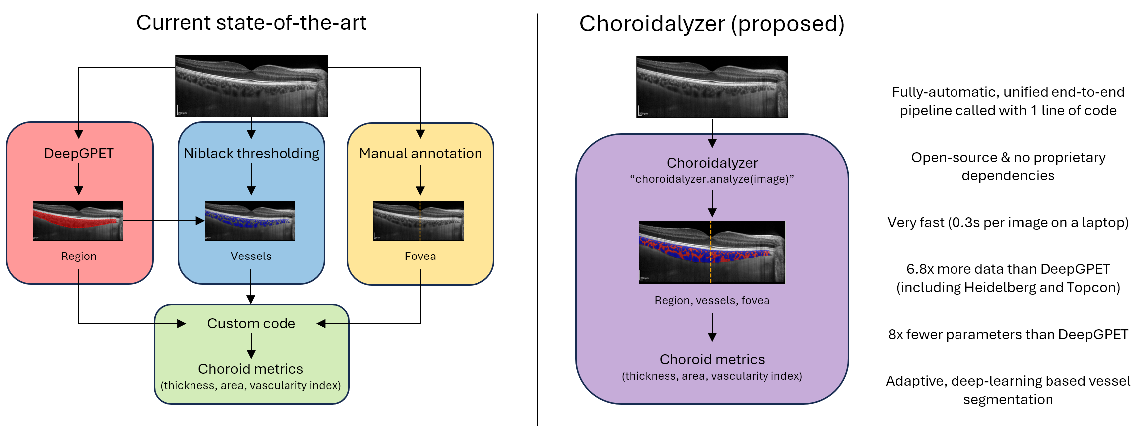
Figure 1: A comparison between Choroidalyzer and the existing state of choroidal analysis. To obtain choroidal metrics in a fovea-centred region of interest, researchers currently need to combine many different tools. Choroidalyzer unifies everything into a end-to-end pipeline that is very fast and convenient to use.

We address these issues by proposing Choroidalyzer, an end-to-end pipeline for choroidal analysis. Choroidalyzer consists of a single deep learning model that simultaneously segments the choroidal region and vessels and detects the fovea location, combined with all the code needed to extract choroidal thickness, area, and vascular index in a fovea-centred region of interest. Fig. 1 shows how Choroidalyzer improves on the current state-of-the-art by providing a comprehensive solution for all elements of choroidal analysis. To our knowledge, Choroidalyzer is the first open-source method for comprehensive, automatic analysis of the choroid from a raw OCT B-scan. Choroidalyzer is highly effective, can be run on a standard laptop in less than one-third of a second per image, does not require any specialist training in image processing and is available on GitHub: https://github.com/justinengelmann/Choroidalyzer.

2 Methods

OCTANE Diurnal Variation Normative i-Test Prevent Dementia GCU Topcon Total Subjects 46 20 1 21 121 24 233 Control/Case 0 / 46 20 / 0 1 / 0 11 / 10 56 / 65 24 / 0 112 / 121 Male/Female 24 / 22 11 / 9 1 / 0 0 / 21 66 / 55 14 / 9 116 / 116 Right/Left eyes 46 / 0 20 / 0 1 / 1 21 / 21 117 / 115 22 / 21 227 / 158 Age (mean (SD)) 47.5 (12.3) 21.4 (2.3) 23.0 (0.0) 32.8 (5.4) 50.8 (5.6) 21.8 (7.9) 42.9 (13.7) Device manufacturer Heidelberg Heidelberg Heidelberg Heidelberg Heidelberg Topcon All Device type Standard Standard FLEX FLEX Standard DRI Triton Plus All Scan location Horizontal/Vertical 168 / 0 55 / 50 4 / 4 76 / 76 381 / 369 132 / 139 816 / 638 Volume/Radial/Peripapillary 0 / 0 / 0 0 / 0 / 66 365 / 0 / 0 2,408 / 0 / 0 0 / 0 / 0 0 / 1,307 / 0 2,773 / 1,307 / 66 Total B-scans 168 171 373 2,560 750 1,578 5,600

Table 1: Overview of population characteristics. SD, standard deviation. Note that one participant’s sex from the GCU Topcon cohort was not recorded.

2.1 Study population

Our dataset contains 5,600 OCT B-scans of 233 participants from 6 cohorts of healthy and diseased individuals, unrelated to ocular pathology; OCTANE[37], a longitudinal cohort study investigating choroidal microvascular changes in renal transplant recipients and healthy donors; Diurnal Variation[37], a sub-cohort of OCTANE of young individuals investigating the possible effects of diurnal variation on the relationship between the choroid and markers of renal function; Normative, a detailed OCT examination of one of the authors (J.B.) with informed consent; i-Test[37], a cohort of pregnant women evaluating whether the choroidal microvasculature reflects cardiovascular changes in both healthy and complicated pregnancies; Prevent Dementia, a longitudinal cohort tracking middle-aged individuals with varying risk of developing late onset Alzheimer’s dementia [38]; GCU Topcon[39], an investigation into diurnal variation of the choroid in emmetropic and myopic individuals. All studies adhered to the Declaration of Helsinki and received relevant ethical approval and informed consent from all subjects was obtained in all cases from the host institution. Table 1 describes the population statistics and image acquisition statistics for each cohort.

Three OCT device types were used from two device manufacturers: the spectral domain OCT SPECTRALIS Standard Module OCT1 system and the spectral domain OCT SPECTRALIS portable FLEX Module OCT2 system (both Heidelberg engineering, Heidelberg, Germany), and the swept source OCT DRI Triton Plus (Topcon, Tokyo, Japan). For the Heidelberg devices, active eye tracking with built-in Automatic Real Time (ART) software was used with horizontal and vertical line scans capturing a 30^∘ (9mm) fovea-centred region of interest, with an ART of 100, i.e. each final B-scan is the average of 100 B-scans. Posterior pole macular line scans covered a 30-by-25-degree rectangular region of interest using 31 consecutive scans, each with an ART of 50 (Posterior pole scans in the Normative cohort were acquired with an ART of 9). All Heidelberg data was collected at a pixel resolution of $768\times 768$ pixels, with a signal quality $\geq$ 15. The Topcon device imaged the macular region using 12 fovea-centred radial scans, spaced 30^∘ apart and covering a 30^∘ (9mm) region of interest. Each B-scan had a resolution of $992\times 1024$ pixels which was cropped horizontally by 32 pixels and resized to the resolution of the Heidelberg scans of $768\times 768$. All Topcon data had an image quality score > 88 determined by the built-in TopQ software.

Five of the six cohorts were split into training (4,144 B-scans, 122 subjects), validation (466 B-scans, 28 subjects) and internal test sets (756 B-scans, 37 subjects) containing approximately 75, 10, and 15% of the B-scans. We split the data on the subject-level, such that no individual ended up in more than one set. The remaining cohort, OCTANE, was entirely held-out as an external test set (168 B-scans, 46 individuals). Supplementary Table S1 gives a detailed overview of population and image characteristics for each of the four sets.

2.2 Ground-truth (GT) labels

The fovea coordinate was defined as the horizontal (column) pixel index which aligned with the deepest point of the foveal pit depression [36], i.e. where the central foveal pit was most illuminated, typically aligning with a ridge formed at the photoreceptor layer. The choroidal region was defined as the space posterior to the boundary delineating the retinal pigment epithelium layer and Bruch’s membrane complex (RPE-Choroid, RPE-C, junction) and superior to the boundary delineating the sclera from the posterior most point of Haller’s layer (Choroid-Sclera, C-S, junction). Between the choroid and sclera lies the suprachoroidal space, which is rarely visible on OCT B-scans and we consider not to be part of the choroid itself. The choroidal space is made up of interstitial fluid, or stroma, seen as brightly illuminated strips in the OCT B-scans, with interspersed, irregular areas of darker intensity representing choroidal vasculature This has been both empirically observed [40, 26] and widely accepted among the research community [29]. The choriocapillaris, a dense network of choroidal capillaries, is seen as a small band below Bruch’s membrane complex approximately 10 microns thick [1] (roughly 3 pixels deep in OCT B-scans), and is assumed as part of the choroidal vasculature alongside larger vessels seen in Haller and Sattler’s layers.

For OCT B-scans centred at the fovea (i.e. horizontal, vertical and radial scans), the foveal column location was detected manually. Those not centred at the fovea do not show the fovea. The GTs for choroidal region segmentation were generated using DeepGPET [25] with the default threshold of 0.5. 897 scans were excluded from the dataset (and removed from Table 1 and supplementary Table S1) because of poor region segmentations — these were primarily Topcon B-scans which DeepGPET had not been trained on before.

GTs for vessel segmentation were generated using a novel, multi-scale quantisation and clustering-based approach, called multi-scale median cut quantisation (MMCQ), which we found to produce superior results to standard application of Niblack in preliminary analysis on the training set. MMCQ segments the choroidal vasculature by performing patch-wise local contrast enhancement at several scales using median cut clustering (quantisation) [41] and histogram equalisation. The pixels of the subsequently enhanced choroidal space are then clustered globally using median cut clustering once more, classifying the pixels belonging to the clusters with the darkest pixel intensities as vasculature. The code for this algorithm is freely available here [LINK TO BE ADDED UPON ACCEPTANCE].

To improve the fidelity and robustness of our vessel segmentation GTs, we randomly varied the brightness and contrast of each OCT B-scan before application of MMCQ. We used 5 linearly spaced gamma levels to fix the mean brightness of each image between 0.2 and 0.5 and simultaneously altered the contrast using 5 linearly spaced factors between 0.5 and 3. A 3:2 majority vote for vessel label classification was used across all 25 variants. This improves robustness as spurious over- and undersegmentation contigent on specific image statistics are averaged out.

2.3 Choroidalyzer’s deep learning model

Choroidalyzer segments the choroid region and vessels, and detects the fovea using a UNet deep learning model [42] with a depth of 7. This relatively high depth allows our model to better consider the global context. The first 3 blocks increase the internal channel dimension from 8 to 64, after which it is kept constant to reduce memory consumption and parameter count. Blocks consist of two convolutional layers, each followed by BatchNorm [43] and ReLU activation. Our up-blocks use a $1\times 1$ convolution to reduce the channel dimension followed by bilinear interpolation, which is more compute and memory efficient than the standard transposed convolutions. We train our model for 40 epochs using the AdamW optimizer [44] with a learning rate of $5\times 10^{-4}$ and weight decay of $10^{-8}$ to minimise binary crossentropy, clamping the maximum gradient norm to $3$ before each step. We use automatic mixed precision to speed up training dramatically while reducing memory consumption by almost half. Forward pass and loss computation are done in bfloat16, a half-precision datatype optimised for machine learning.

During training, we apply the following data augmentations in random order per sample: Horizontal flip ($p=0.5$), changing the brightness and contrast independently (factors $\sim U(0.5,1.5)$, $p=0.95$), random rotation and shear (degrees $\sim U(-25,25)$ and $\sim U(-15,15)$ respectively, $p=\nicefrac{{1}}{{3}}$), scaling the image (factor $\sim U(0.8,1.2)$, $p=\nicefrac{{1}}{{3}}$), where $U(a,b)$ denotes a uniform distribution between $a$ and $b$, and $p$ the probability of the transform being applied. For peripapillary scans which have a resolution of $1536\times 768$, we use a crop of $768\times 768$ using a random multiple of $192$ as offset per example and epoch.

The fovea is only a single point which would be difficult for a segmentation model to learn, as predicting close to 0 for all pixels would yield virtually the same loss as a perfect prediction. Thus, we create a target 51 pixels high and 19 pixels wide centred at the GT fovea location. The exact fovea location is set to 1, the whole column to 0.95, and adjacent columns to $0.95-(d*0.1)$ where d is the column distance from the fovea. Finally, we employ one-sided label smoothing and set all other pixels to 0.01 instead of 0 to stabilise training. We extract fovea column predictions by applying a 21-width triangular filter to the column-wise sums of our model’s predictions and taking the column with the highest value.

2.4 Statistical analysis

We evaluate agreement in segmentations using the area under the receiver operating characteristic curve (AUC) and Dice coefficient, applying a fixed threshold of 0.5 to binarize our model’s predictions. For the fovea column location, we use mean absolute error (MAE) and median absolute error (Median AE). For derived choroid metrics, we evaluate agreement with Pearson and Spearman correlations and further report MAEs.

All choroidal metrics were computed using a region of interest (ROI) centred at the foveal pit, measuring 3mm temporally and nasally — the ROI for volume scans was centred at the middle column index of the image — corresponding to the standardised ROI according to the Early Treatment Diabetic Retinopathy Study (ETDRS) macular grid of 6,000 $\times$ 6,000 microns [45]. As peripapillary scans do not allow for a fovea-centred region of interest, we only look at segmentation metrics and use a threshold of 0.25 for vessel predictions. Area was computed by counting the pixels within the ETDRS grid, while thickness was measured at three linearly spaced locations, spanning the ETDRS grid, as point-source micron distances between the RPE-C and C-S junctions, locally perpendicular to the RPE-C junction.

Choroid vascular index is the ratio of vessel to non-vessel pixels in the choroid within the ETDRS grid. Our deep learning model outputs probabilities instead of discrete predictions, which capture uncertainty. As capturing uncertainty is desirable, we propose a “soft” vascular index which takes the ratio of predicted probabilities instead of discretized binary predictions. On the validation set, we found that this improves agreement.

To examine and characterise the behaviour of our model, we analysed cases of high error in detail. Concretely, for each of the three tasks (region and vessel segmentation, fovea detection), we selected the 15 examples from each test set where Choroidalyzer produced the highest errors. For redundant cases (i.e. adjacent, highly-similar slices from a volume scan) only one was retained. For fovea detection, cases of low error were also discarded. This left 28 cases for region, 29 for vessel, and 25 for fovea.

An adjudicating clinical ophthalmologist (I.M.) was provided with the original image, Choroidalyzer’s prediction and the GT while being masked to the identity of the methods. Images and labels were provided individually and as composites. For each example, the adjudicator was asked which label they preferred. They also rated each label qualitatively on a 5-level ordinal scale (“Very bad”, “Bad”, “Okay”, “Good” and “Very good”) for region segmentation quality, as well as intravascular and interstitial vessel segmentation quality. The latter two to quantify any potential under-segmentation of vessels and over-segmentation of the interstitial space.

Finally, we selected a random subsample of 20 B-scans at the patient-level from the external test set to be manually segmented by two graders, M1 and M2. M1 was a clinical ophthalmologist (I.M.) and M2 was a a PhD student who has worked with choroidal OCT data for the last 4 years (J.B.). Manual graders segmented the region and choroidal vessels using ITK-Snap [46]. The manual segmentations were compared to Choroidalyzer and to the current state-of-the-art, namely DeepGPET for region segmentations [25] and Niblack for vessel segmentation using a window size of 51 and standard deviation offset of -0.05, which mirrors previously published work [33].

3 Results

Set Region Vessel Fovea Thickness Area Vascular Index AUC Dice AUC Dice MAE Median AE pearson spearman MAE ($\mu$m) pearson spearman MAE (mm²) pearson spearman MAE Internal test 0.9998 0.9789 0.9982 0.8817 3.9 px 3.0 px 0.9754^∗∗∗ 0.9692^∗∗∗ 8.2252 0.9815^∗∗∗ 0.9786^∗∗∗ 0.0385 0.8285^∗∗∗ 0.8097^∗∗∗ 0.0206 External test 0.9998 0.9749 0.9980 0.8703 3.4 px 3.0 px 0.9831^∗∗∗ 0.9868^∗∗∗ 8.0888 0.9779^∗∗∗ 0.9848^∗∗∗ 0.0487 0.7948^∗∗∗ 0.7991^∗∗∗ 0.0306

Table 2: Metrics for Choroidalyzer against ground-truth annotations from the internal and external test sets. ^∗∗∗ indicates p<0.0001.

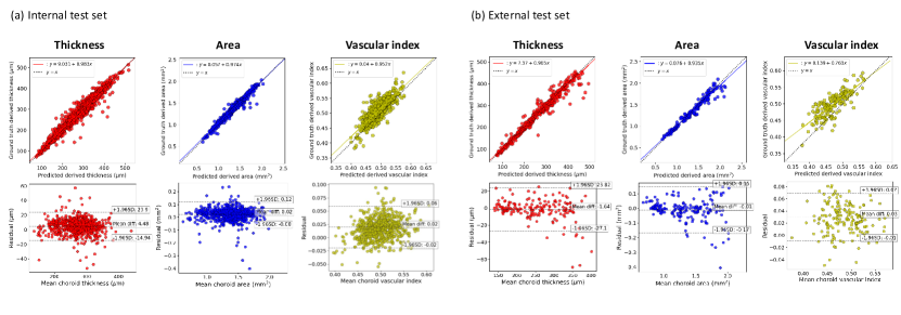
Figure 2: Agreement in thickness, area and vascular index for a) the internal and b) the external test sets. Top row are scatterplots with best regression fit and identity lines, bottom row are Bland-Altman plots. Note that we chose to fit each plot to the data range and thus the scale of the axes are not exactly the same between internal and external test sets, especially for vascular index.

3.1 Performance on internal and external test sets

Table 2 shows the performance of Choroidalyzer on the internal and external test sets. Our model achieves very good performance in terms of AUC and Dice for region and vessels on both sets. Metrics for region are higher than for vessels, which is expected as choroidal vessel segmentation is much more difficult and ambiguous than region segmentation, and thus the GTs are themselves imperfect. Performance was slightly higher for the internal test set than the external test set, which is expected, but only marginally so, indicating that our model generalises well to new cohorts. For the peripapillary scans which only exist in the internal test set, our model achieved an AUC of 0.9996 (region) / 0.9925 (vessel) and Dice of 0.9636 (region) / 0.7155 (vessel). This is reasonable performance but lower than for other scans.

For fovea detection, the model had a MAE of 3.9 px for the internal and 3.4 px for the external test set, with the median absolute error being 3 px for both. This is excellent performance as an error of 3 px on a 768 px-wide image will not meaningfully change our region-of-interest or resulting metrics (data not shown — see the supplementary materials for the analysis effects of fovea location on downstream metrics). For the derived choroid metrics, Choroidalyzer shows excellent agreement with the GTs on thickness and area, with Pearson and Spearman correlations of 0.9692 or greater for both internal and external test sets. For the vascular index, performance is a bit lower, with correlations between 0.7948 and 0.8285. Although vascular index depends on both region and vessel segmentation, the other metrics indicate that the differences in vascular index are driven primarily by differences in vessel segmentation. Still, the observed correlations are high in absolute terms. Fig. 2 shows correlation and Bland-Altman plots for the three derived metrics on both test sets, which likewise indicate generally very good agreement. Fig. 3 shows some examples for each of the three imaging devices.

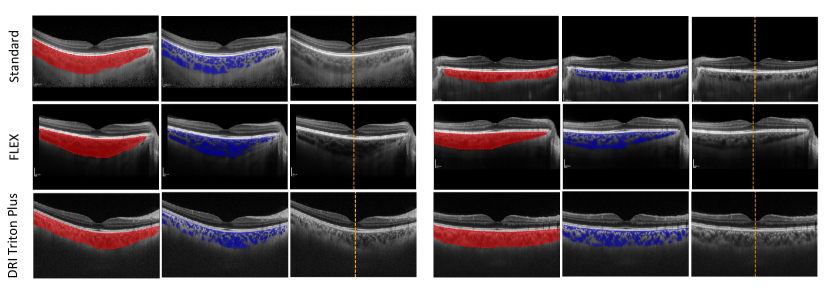
Figure 3: Examples of Choroidalyzer being applied to scans from different imaging devices. Six fovea-centred OCT B-scans, two per imaging device type, from the internal test set showing region segmentations (left), vessel segmentations (middle), and fovea column location (right).

3.2 Comparison with manual segmentations

Table 3 shows the results from manual segmentations. For automated methods, we compare with each manual grader and then averaged the performance across both graders to make the results more concise. The comparisons with individual graders are reported in the supplementary Table S2. Interestingly, while vessel Dice for Choroidalyzer (0.7410 vs M1 and 0.7927 vs M2; mean 0.7669) is again much worse than region Dice and even worse than the vessel Dice on both test sets, it is very similar to the inter-grader agreement of 0.7699. More generally, the inter-grader agreements for all other metrics are similar to Choroidalyzer’s agreement with the graders, with the notable exception of vascular index. Here, Choroidalyzer’s MAE is better (0.0555 vs M1 and 0.0506 vs M2; mean 0.0531) than the inter-grader agreement (0.0618), as is the Spearman correlation, but Pearson correlation and ICC are worse. Compared to the respective state-of-the-art (SOTA, i.e. DeepGPET for region, Niblack for vessel segmentation), Choroidalyzer has better agreement with the graders for most of the metrics, although methods are generally comparable.

Table 4 shows the time per scan for the manual graders and automatic approaches. The manual graders on average needed more than 26 and 22 minutes (mean 24), with the vast majority of that time spent on the vessel segmentation. By contrast, the automatic methods on a standard laptop needed about a second per scan and no human time at all. Thus, to get through a dataset of 100 scans, it would take manual graders about 40 hours of work, but with automated methods it would be less than 2 minutes. With GPU-acceleration, Choroidalyzer and DeepGPET could achieve throughputs of dozens or hundreds of scans per second even on consumer-grade hardware. Comparing the automated methods with each other, Choroidalyzer took 73% less time than DeepGPET and Niblack, while also detecting the fovea location. All three methods are very fast but for very large datasets or deployment on edge devices, Choroidalyzer’s efficiency is an additional advantage over existing automated methods.

Comparison Region Vessel Thickness Area Vascular Index AUC Dice AUC Dice pearson spearman ICC MAE ($\mu$m) pearson spearman ICC MAE (mm²) pearson spearman ICC MAE M1 vs. M2 0.9639 0.9474 0.8891 0.7699 0.9503 0.9521 0.9783 17.8833 0.9516 0.9248 0.9751 0.1096 0.8074 0.6857 0.8172 0.0618 Choroidalyzer vs. Manual (avg) 0.9978 0.9375 0.9914 0.7669 0.9534 0.9663 0.9873 20.9750 0.9554 0.9368 0.9756 0.1150 0.6654 0.7383 0.7613 0.0530 SOTA vs. Manual (avg) 0.9444 0.9333 0.9223 0.7742 0.9676 0.9636 0.9802 19.9250 0.9548 0.9233 0.9769 0.1202 0.6907 0.6105 0.7103 0.1682

Table 3: Comparison metrics for the 20 images assessed manually and algorithmically from the external test set. Comparisons made between the 2 manual graders, the proposed model and current state of the art, DeepGPET for region segmentation and the Niblack thresholding algorithm for vessel segmentation. SOTA: current state-of-the-art, i.e. DeepGPET for region and Niblack for vessel segmentation.

     Method    Region (s)     Vessel (s)     Total (s) M1 78.400 $\pm$ 12.261 1506.000 $\pm$ 744.073 1584.400 $\pm$ 771.284 M2 165.000 $\pm$ 23.889 1176.700 $\pm$ 744.073 1341.700 $\pm$ 265.800 SOTA 0.751 $\pm$ 0.081 0.370 $\pm$ 0.105 1.121 $\pm$ 0.140 Choroidalyzer - - 0.299 $\pm$ 0.018

Table 4: Mean (standard deviation) execution time of the four different approaches to region and vessel segmentation for the 20 images assessed manually and algorithmically from the external test set. SOTA: current state-of-the-art, i.e. DeepGPET for region and Niblack for vessel segmentation. Automated methods were run on a standard laptop with a 4 year old i5 CPU and 16 GB of RAM but no GPU.

3.3 Detailed error analysis

Preferred Choroidalyzer Preferred SOTA Both equally good Region 8/28 5/28 15/28 Vessel 13/29 4/29 12/29 Fovea 23/25 1/25 1/25 Method Region: quality Vessel: intravascular Vessel: interstitial Choroidalyzer VG: 3, G: 14, O: 9, B: 1, VB: 1 VG: 0, G: 17, O: 12, B: 0, VB: 0 VG: 0, G: 20, O: 9, B: 0, VB: 0 SOTA VG: 0, G: 17, O: 8, B: 1, VB: 2 VG: 0, G: 5, O: 19, B: 3, VB: 2 VG: 0, G: 17, O: 8, B: 2, VB: 2

Table 5: Preference and segmentation scores from masked expert adjudicator (I.M.) comparing the highest region segmentation, vessel segmentation and fovea column errors between Choroidalyzer and the ground truth labels. VG, very good; G, good; O, okay; B, bad; VB, very bad.

Table 5 shows the results of manual inspection of scans where Choroidalyzer produced the highest error compared to the GT on the test sets. For region segmentation, Choroidalyzer was preferred in 8 cases, the GT in 5, and both methods were considered equally good in 15 cases. In terms of quality, Choroidalyzer was “Very bad” in only one case compared with 2 for the GT and “Very good” 3 times compared to none for the GT. For the vessels, Choroidalyzer was preferred in 13 cases, the GT in 4, and both were tied in 12 cases. Vessel segmentation is a harder task, with no methods achieving “Very good”. However, the intravascular scores for Choroidalyzer are substantially better, with no “Bad” or “Very bad” (vs. 3 and 2, respectively for GT) and far more “Good” (17 vs. 5), and the interstitial scores are similarly better. Finally, for the fovea, Choroidalyzer was preferred 23/25 times and the GT only twice, indicating that large fovea errors are almost exclusively due to mistakes in the manual GT labels.

Fig. 4 shows the distributions of fovea errors for both test sets along with each example in both sets. For very large residuals (10+px), the GTs are wrong and Choroidalyzer correctly identifies the fovea location. For errors around 7px, still twice the MAE, both methods are similar with either method sometimes being more correct. Further exploration revealed the majority of incorrectly labelled ground-truths to be Topcon OCT B-scans, as each 12-stack of radial scans are not centred at the fovea, and initial manual annotation detected the fovea for only one to represent each stack. Despite this oversight, Choroidalyzer learned to dectect the fovea robust and accurately.

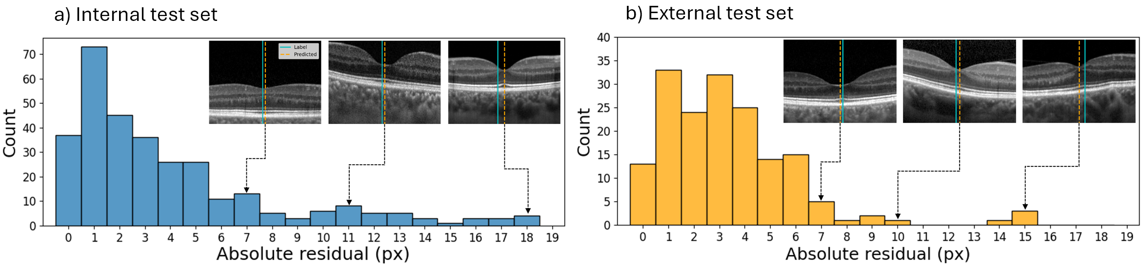
Figure 4: Histogram of absolute errors for fovea column detection for the internal (left) and external (right) test sets. Examples for different levels of error are shown with dotted lines indicating which part of the distribution they come from. In the examples, the teal line indicates the GT label, the dashed orange line the prediction.

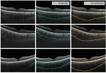
Figure 5: Three example Topcon OCT B-scans with successful region segmentations from Choroidalyzer (right) and failed segmentations from DeepGPET (middle).

4 Discussion

We developed Choroidalyzer, an end-to-end pipeline for choroidal analysis. Choroidalyzer shows excellent performance on the internal and external test sets. Where Choroidalyzer produced the highest errors were primarily cases of imperfect GTs and Choroidalyzer was generally preferred by a blinded adjudicating ophthalmologist (I.M.), further indicating robustness and good performance. Its agreement with manual segmentations, which demand substantial time and attention from a human expert, is comparable to the inter-grader agreement. This suggests that Choroidalyzer performs well compared to laborious manual segmentation and also highlights the subjectivity introduced by manual graders. Choroidalyzer not only produces results similar to that of a skilled manual grader, it also does so fully-automatically without introducing subjectivity and thus increases standardisation and reproducibility. If researchers use Choroidalyzer, their results are repeatable and would be much more comparable to other studies also using Choroidalyzer than if different manual graders were used in each case.

Additionally, Choroidalyzer saves a substantial amount of time per image over manual segmentation, freeing up researcher time and enabling large scale analyses that otherwise would not be possible. Even compared to the current state-of-the-art for automated methods, DeepGPET and Niblack, Choroidalyzer can do the analysis in roughly a quarter of the time. More importantly, Choroidalyzer provides an end-to-end pipeline which makes it easier to implement and use than having to combine multiple methods like Niblack and DeepGPET. Ease-of-use is often underappreciated in the literature but key in saving researchers time and allowing them to focus on the science.

Choroidalyzer performed well against manual graders relative to the state of the art methods, reaching or surpassing the levels of agreement even between the two manual graders, particularly for vascular index, a far more difficult metric to calculate accurately than area and thickness. The inter-grader agreement between manual graders for these metrics indicate a potential lower bound of what effect sizes we might expect from these metrics. This has important downstream impact on the statistical confidence of results from cohort studies, particularly when assessing the choroidal vasculature [31, 28].

It is often difficult to visualise the choroid due to imaging noise, poor eye tracking and patient fixation, or operator inexperience. Thus, in some cases vessel boundaries can be hard to discern. This is why we proposed to use a soft version of choroid vascular index where the probabilities that Choroidalyzer outputs are used instead of thresholded, binarized segmentations. The probabilities capture uncertainty about the precise location of the vessel wall and thus is more robust than using a single, somewhat arbitrary threshold. Users could also tune the binarization threshold for their own images, if desired, which might help in instances of poor visibility of the choroidal vasculature.

Segmentation performance for peripapillary scans was reasonable but much worse than for other scan types. This could be due to those scans being relatively rare in our dataset and showing parts of the retina on the nasal side of the optic disc that are not captured in fovea-centred scans. More peripapillary training data would likely increase performance. In our opinion, at present Choroidalyzer can be used for these scans but requires subsequent manual inspection and potential correction. Furthermore, adjusting the binarization threshold for the vessel predictions can improve results.

Our model detected the fovea well, and the largest errors were cases where ground-truths were incorrectly labelled with the model correctly identifying the fovea location as confirmed by masked adjudication. Thus, the model performed even better than what the quantitative results suggest. In the present work, we have focused on identifying the fovea column which is needed to define the fovea-centred region of interest. However, after selecting and evaluating our final model, we realised that in relatively rare, highly myopic cases, the retina and choroid can be at a steep angle relative to the image axes. For those, it would be best to define the region of interest along the choroid axes rather than image axes, most easily done by drawing a centre line from the fovea perpendicularly through the retina and choroid. Thus, it could be useful to also segment the retina and to determine both the row and column of the fovea. While not our initial objective, we did some preliminary analyses and found that we can derive the fovea row well with our current model (data not shown). Furthermore, to understand the effect of fovea location error on downstream choroidal metrics, we simulated random per-sample deviations of $\pm 6$px, twice the Median AE, and found that they yielded virtually identical results (see supplementary Fig. S1 and Fig. S2).

The dataset in the present work was substantially larger than the one used for DeepGPET and importantly contains both Heidelberg and Topcon scans. As a result, Choroidalyzer can segment even difficult Topcon scans where DeepGPET failed (Fig. 5). Choroidalyzer was trained on region and vessel GTs generated by fully- and semi-automatic methods, respectively, which were then checked for errors and only manually improved where needed. Recent work argues that such approaches to generating GTs are preferable as they reduce subjectivity and thus bias and inconsistency[47].

Choroidalyzer also has limitations. Most importantly, there is no quality scoring component to reject B-scans that do not show the choroid in sufficient detail to allow for reasonable analysis. While modern OCT devices typically show the choroid in good detail, especially if EDI is used, this is not always the case. Most devices provide some quality indicators, but we have not investigated quality thresholds for specific devices, below which Choroidalyzer would not function. Furthermore, OCT quality indicators are typically focused on the retina, and although poor visualisation of the retina might imply poor visualisation of the choroid, the reverse is not necessarily the case. A quality scoring method specific to the choroid would be a useful addition to the field. Another limitation is that Choroidalyzer was trained only on cohorts relating to systemic health but not ocular disease or data acquired during routine clinical practice.

Future work could improve the underlying deep learning model of Choroidalyzer, e.g. by training and evaluating it on data from more diverse sources. Data with ocular pathology, e.g. abnormally sized choroids due to myopia, age-related macular degeneration or central serous chorio-retinopathy, could be used to investigate whether Choroidalyzer is robust in those contexts and to train an improved version if needed. Moreover, automated quality scoring methods relating to the choroid would address a key need in choroidal analysis. Finally, Choroidalyzer could be extended to measure additional choroidal metrics, such as macular thickness and vessel density maps across a volume, or relating to its curvature.

5 Conclusion

Choroidal thickness, area, and especially vascular index are highly interesting metrics and potential biomarkers for both systemic and ocular health. However, calculating them used to be laborious and - when done manually - subjective. Choroidalyzer provides an efficient, end-to-end pipeline to alleviate these problems. We hope that by making Choroidalyzer openly accessible, we will enable researchers and clinicians to conveniently calculate these metrics and use them for their research, while improving reproducibility and standardisation in the field.

6 Conflicts of Interest

The authors declare no conflicts of interest.

Supplementary Material

	Training	Validation	Testing	External test	Total
Subjects	122	28	37	46	233
Male/Female	64 / 57	12 / 16	16 / 21	24 / 22	116 / 116
Control/Case	76 / 46	16 / 12	20 / 17	0 / 46	112 / 121
Right/Left eyes	117 / 107	27 / 23	37 / 28	46 / 0	227 / 158
Standard/FLEX/DRI Triton Plus	88 / 14 / 20	24 / 2 / 2	29 / 6 / 2	46 / 0 / 0	187 / 22 / 24
Heidelberg/Topcon	102 / 20	26 / 2	35 / 2	46 / 0	209 / 24
Age (mean (SD))	40.7 (14.2)	42.5 (11.9)	44.5 (13.4)	47.5 (12.3)	42.9 (13.4)
Cohort
OCTANE	0	0	0	46	46
Diurnal Variation	12	4	4	0	20
Normative	1	0	0	0	1
i-Test	13	2	6	0	21
Prevent Dementia	76	20	25	0	121
GCU Topcon	20	2	2	0	24
B-scans
Standard/Flex/DRI Triton Plus	582 / 2,281 / 1,281	136 / 190 / 140	137 / 462 / 157	168 / 0 / 0	1,023 / 2,933 / 1,578
Heidelberg/TopCon	2,863 / 1,281	326 / 140	599 / 157	168 / 0	3,956 / 1,578
Horizontal/Vertical scans	462 / 461	90 / 82	95 / 95	168 / 0	816 / 638
Volume/Radial/Peripapilary scans	2,161 / 1,060 / 39	178 / 116 / 15	434 / 131 / 12	0 / 0 / 0	2,773 1,307 / 0
Total B-scans	4,183	481	768	168	5,600

Table S1: Overview of population and image characteristics of the internal training, validation and test sets, and also the external test set. Note that one participant’s sex from the Topcon cohort was not recorded.

Comparison Region Vessel Thickness Area Vascular Index AUC Dice AUC Dice pearson spearman ICC MAE ($\mu$m) pearson spearman ICC MAE (mm²) pearson spearman ICC MAE M1 vs. M2 0.9639 0.9474 0.8891 0.7699 0.9503 0.9521 0.9783 17.8833 0.9516 0.9248 0.9751 0.1096 0.8074 0.6857 0.8172 0.0618 M1 Choroidalyzer 0.9964 0.9242 0.9896 0.7410 0.9322 0.9490 0.9761 27.2167 0.9211 0.8872 0.9570 0.1598 0.7668 0.8406 0.7265 0.0555 SOTA 0.9370 0.9227 0.9271 0.7714 0.9437 0.9378 0.9676 25.8500 0.9198 0.8692 0.9589 0.1631 0.7150 0.6857 0.7157 0.1901 M2 Choroidalyzer 0.9993 0.9507 0.9933 0.7927 0.9746 0.9838 0.9984 14.7333 0.9896 0.9865 0.9942 0.0702 0.5640 0.6361 0.7960 0.0506 SOTA 0.9175 0.9439 0.9175 0.7770 0.9914 0.9894 0.9927 14.0000 0.9897 0.9774 0.9948 0.0770 0.6663 0.5353 0.7047 0.1464

Table S2: Full comparison metrics between Choroidalyzer, two manual graders M1 and M2, and state of the art region and vessel segmentation methods DeepGPET and Niblack.

6.1 Analysis effects of fovea location error on downstream metrics

Choroidalyzer measured the fovea column coordinate with a median absolute error of 3 pixels in both the internal and external test sets. We tested the effect of perturbing the fovea column on choroidal metrics by comparing fovea-centred metrics and metrics derived after the fovea column was randomly perturbed using a discretised uniform distribution $\sim U(-6,6\}$ (excluding 0). 50 simulations were run on approximately 10% of the dataset (495 OCT B-scans), selected at random to represent eye type and location on the macula. All metrics had excellent Pearson correlation ($r$ > 0.99, p<0.00001, supplementary Fig. S1). Scatterplots of metrics for the poorest performing simulation according to absolute error across all metrics (supplementary Fig. S2) shows excellent agreement with the identity line, with limits of agreement in the Bland-Altman plots well within acceptable bounds for all metrics [48, 49]. Thus, the fovea column quantitative error observed from Choroidalyzer does not significantly impact the choroidal metrics.

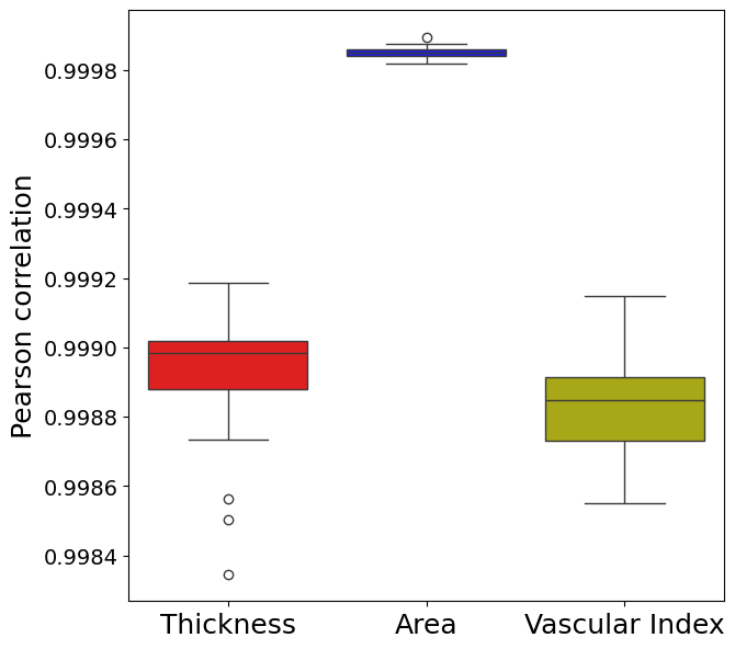
Figure S1: Distribution of Pearson correlation coefficients for each choroidal metric when perturbing the fovea coordinate column. Note the scale of the y-axis, even the lowest correlation we observed was $>0.99$.

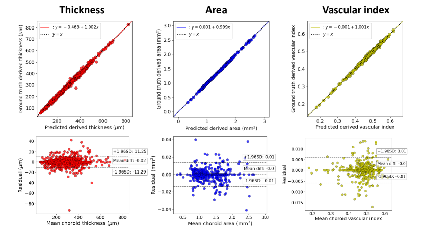
Figure S2: Correlation and Bland-Altman plots for choroidal metrics for the poorest performing simulation of perturbing the fovea column coordinate on a random 10% subsample of the dataset.

References

- [1] Debora L Nickla and Josh Wallman. The multifunctional choroid. Progress in retinal and eye research, 29(2):144–168, 2010.
- [2] Cason B Robbins, Dilraj S Grewal, Atalie C Thompson, James H Powers, Srinath Soundararajan, Hui Yan Koo, Stephen P Yoon, Bryce W Polascik, Andy Liu, Rupesh Agrawal, et al. Choroidal structural analysis in alzheimer disease, mild cognitive impairment, and cognitively healthy controls. American Journal of Ophthalmology, 223:359–367, 2021.
- [3] Craig Balmforth, Job JMH van Bragt, Titia Ruijs, James R Cameron, Robert Kimmitt, Rebecca Moorhouse, Alicja Czopek, May Khei Hu, Peter J Gallacher, James W Dear, et al. Chorioretinal thinning in chronic kidney disease links to inflammation and endothelial dysfunction. JCI insight, 1(20), 2016.
- [4] Shanna C Yeung, Yuyi You, Kathryn L Howe, and Peng Yan. Choroidal thickness in patients with cardiovascular disease: a review. Survey of ophthalmology, 65(4):473–486, 2020.
- [5] Scott A Read, James A Fuss, Stephen J Vincent, Michael J Collins, and David Alonso-Caneiro. Choroidal changes in human myopia: insights from optical coherence tomography imaging. Clinical and Experimental Optometry, 102(3):270–285, 2019.
- [6] Jamie Burke, Dan Pugh, Tariq Farrah, Charlene Hamid, Emily Godden, Thomas J. MacGillivray, Neeraj Dhaun, J. Kenneth Baillie, Stuart King, and Ian J. C. MacCormick. Evaluation of an Automated Choroid Segmentation Algorithm in a Longitudinal Kidney Donor and Recipient Cohort. Translational Vision Science & Technology, 12(11):19–19, 11 2023.
- [7] Jamie Burke, Neeraj Dhaun, Baljean Dhillon, Kyle J Wilson, Nicholas AV Beare, and Ian JC MacCormick. The retinal contribution to the kidney–brain axis in severe malaria. Trends in parasitology, 2023.
- [8] Yong Un Shin, Sang Eun Lee, Min Ho Kang, Sang-Woong Han, Joo-Hark Yi, and Heeyoon Cho. Evaluation of changes in choroidal thickness and the choroidal vascularity index after hemodialysis in patients with end-stage renal disease by using swept-source optical coherence tomography. Medicine, 98(18), 2019.
- [9] Anita Kundu, Justin P Ma, Cason B Robbins, Praruj Pant, Vithiya Gunasan, Rupesh Agrawal, Sandra Stinnett, Burton L Scott, Kathryn PL Moore, Sharon Fekrat, et al. Longitudinal analysis of retinal microvascular and choroidal imaging parameters in parkinson’s disease compared with controls. Ophthalmology Science, page 100393, 2023.
- [10] Richard F Spaide, Hideki Koizumi, and Maria C Pozonni. Enhanced depth imaging spectral-domain optical coherence tomography. American journal of ophthalmology, 146(4):496–500, 2008.
- [11] Kara-Anne Tan, Preeti Gupta, Aniruddha Agarwal, Jay Chhablani, Ching-Yu Cheng, Pearse A Keane, and Rupesh Agrawal. State of science: choroidal thickness and systemic health. Survey of ophthalmology, 61(5):566–581, 2016.
- [12] Jamie Burke and Stuart King. Edge tracing using gaussian process regression. IEEE Transactions on Image Processing, 31:138–148, 2021.
- [13] Reza Alizadeh Eghtedar, Mahdad Esmaeili, Alireza Peyman, Mohammadreza Akhlaghi, and Seyed Hossein Rasta. An update on choroidal layer segmentation methods in optical coherence tomography images: a review. Journal of Biomedical Physics & Engineering, 12(1):1, 2022.
- [14] Saleha Masood, Bin Sheng, Ping Li, Ruimin Shen, Ruogu Fang, and Qiang Wu. Automatic choroid layer segmentation using normalized graph cut. IET Image Processing, 12(1):53–59, 2018.
- [15] Bahareh Salafian, Rahele Kafieh, Abdolreza Rashno, Mohsen Pourazizi, and Saeid Sadri. Automatic segmentation of choroid layer in edi oct images using graph theory in neutrosophic space. arXiv preprint arXiv:1812.01989, 2018.
- [16] Vedran Kajić, Marieh Esmaeelpour, Boris Považay, David Marshall, Paul L Rosin, and Wolfgang Drexler. Automated choroidal segmentation of 1060 nm oct in healthy and pathologic eyes using a statistical model. Biomedical optics express, 3(1):86–103, 2012.
- [17] Chuang Wang, Ya Xing Wang, and Yongmin Li. Automatic choroidal layer segmentation using markov random field and level set method. IEEE journal of biomedical and health informatics, 21(6):1694–1702, 2017.
- [18] Nizampatnam Srinath, A Patil, V Kiran Kumar, Soumya Jana, Jay Chhablani, and Ashutosh Richhariya. Automated detection of choroid boundary and vessels in optical coherence tomography images. In 2014 36th Annual International Conference of the IEEE Engineering in Medicine and Biology Society, pages 166–169. IEEE, 2014.
- [19] Neetha George and CV Jiji. Two stage contour evolution for automatic segmentation of choroid and cornea in oct images. Biocybernetics and biomedical Engineering, 39(3):686–696, 2019.
- [20] Hajar Danesh, Raheleh Kafieh, Hossein Rabbani, and Fedra Hajizadeh. Segmentation of choroidal boundary in enhanced depth imaging octs using a multiresolution texture based modeling in graph cuts. Computational and mathematical methods in medicine, 2014, 2014.
- [21] Javier Mazzaferri, Luke Beaton, Gisèle Hounye, Diane N Sayah, and Santiago Costantino. Open-source algorithm for automatic choroid segmentation of oct volume reconstructions. Scientific reports, 7(1):42112, 2017.
- [22] Jason Kugelman, David Alonso-Caneiro, Scott A Read, Jared Hamwood, Stephen J Vincent, Fred K Chen, and Michael J Collins. Automatic choroidal segmentation in oct images using supervised deep learning methods. Scientific reports, 9(1):13298, 2019.
- [23] Sripad Krishna Devalla, Prajwal K Renukanand, Bharathwaj K Sreedhar, Giridhar Subramanian, Liang Zhang, Shamira Perera, Jean-Martial Mari, Khai Sing Chin, Tin A Tun, Nicholas G Strouthidis, et al. Drunet: a dilated-residual u-net deep learning network to segment optic nerve head tissues in optical coherence tomography images. Biomedical optics express, 9(7):3244–3265, 2018.
- [24] Hung-Ju Chen, Yu-Len Huang, Siu-Lun Tse, Wei-Ping Hsia, Chung-Hao Hsiao, Yang Wang, and Chia-Jen Chang. Application of artificial intelligence and deep learning for choroid segmentation in myopia. Translational Vision Science & Technology, 11(2):38–38, 2022.
- [25] Jamie Burke, Justin Engelmann, Charlene Hamid, Megan Reid-Schachter, Tom Pearson, Dan Pugh, Neeraj Dhaun, Stuart King, Tom MacGillivray, Miguel O. Bernabeu, Amos Storkey, and Ian J. C. MacCormick. An open-source deep learning algorithm for efficient and fully-automatic analysis of the choroid in optical coherence tomography, 2023.
- [26] Lauren A Branchini, Mehreen Adhi, Caio V Regatieri, Namrata Nandakumar, Jonathan J Liu, Nora Laver, James G Fujimoto, and Jay S Duker. Analysis of choroidal morphologic features and vasculature in healthy eyes using spectral-domain optical coherence tomography. Ophthalmology, 120(9):1901–1908, 2013.
- [27] Shozo Sonoda, Taiji Sakamoto, Takehiro Yamashita, Makoto Shirasawa, Eisuke Uchino, Hiroto Terasaki, and Masatoshi Tomita. Choroidal structure in normal eyes and after photodynamic therapy determined by binarization of optical coherence tomographic images. Investigative ophthalmology & visual science, 55(6):3893–3899, 2014.
- [28] Rupesh Agrawal, Preeti Gupta, Kara-Anne Tan, Chui Ming Gemmy Cheung, Tien-Yin Wong, and Ching-Yu Cheng. Choroidal vascularity index as a measure of vascular status of the choroid: measurements in healthy eyes from a population-based study. Scientific reports, 6(1):21090, 2016.
- [29] Rupesh Agrawal, Jianbin Ding, Parveen Sen, Andres Rousselot, Amy Chan, Lisa Nivison-Smith, Xin Wei, Sarakshi Mahajan, Ramasamy Kim, Chitaranjan Mishra, et al. Exploring choroidal angioarchitecture in health and disease using choroidal vascularity index. Progress in retinal and eye research, 77:100829, 2020.
- [30] Bjorn Kaijun Betzler, Jianbin Ding, Xin Wei, Jia Min Lee, Dilraj S Grewal, Sharon Fekrat, Srinivas R Sadda, Marco A Zarbin, Aniruddha Agarwal, Vishali Gupta, et al. Choroidal vascularity index: a step towards software as a medical device. British Journal of Ophthalmology, 106(2):149–155, 2022.
- [31] Xin Wei, Shozo Sonoda, Chitaranjan Mishra, Neha Khandelwal, Ramasamy Kim, Taiji Sakamoto, and Rupesh Agrawal. Comparison of choroidal vascularity markers on optical coherence tomography using two-image binarization techniques. Investigative Ophthalmology & Visual Science, 59(3):1206–1211, 2018.
- [32] Xiaoxiao Liu, Lei Bi, Yupeng Xu, Dagan Feng, Jinman Kim, and Xun Xu. Robust deep learning method for choroidal vessel segmentation on swept source optical coherence tomography images. Biomedical Optics Express, 10(4):1601–1612, 2019.
- [33] Joshua Muller, David Alonso-Caneiro, Scott A Read, Stephen J Vincent, and Michael J Collins. Application of deep learning methods for binarization of the choroid in optical coherence tomography images. Translational Vision Science & Technology, 11(2):23–23, 2022.
- [34] Gu Zheng, Yanfeng Jiang, Ce Shi, Hanpei Miao, Xiangle Yu, Yiyi Wang, Sisi Chen, Zhiyang Lin, Weicheng Wang, Fan Lu, et al. Deep learning algorithms to segment and quantify the choroidal thickness and vasculature in swept-source optical coherence tomography images. Journal of Innovative Optical Health Sciences, 14(01):2140002, 2021.
- [35] Tin Tin Khaing, Takayuki Okamoto, Chen Ye, Md Abdul Mannan, Hirotaka Yokouchi, Kazuya Nakano, Pakinee Aimmanee, Stanislav S Makhanov, and Hideaki Haneishi. Choroidnet: a dense dilated u-net model for choroid layer and vessel segmentation in optical coherence tomography images. IEEE Access, 9:150951–150965, 2021.
- [36] Meng Xuan, Wei Wang, Danli Shi, James Tong, Zhuoting Zhu, Yu Jiang, Zongyuan Ge, Jian Zhang, Gabriella Bulloch, Guankai Peng, et al. A deep learning–based fully automated program for choroidal structure analysis within the region of interest in myopic children. Translational Vision Science & Technology, 12(3):22–22, 2023.
- [37] Neeraj Dhaun. Optical coherence tomography and nephropathy: The octane study. https://clinicaltrials.gov/ct2/show/NCT02132741, 2014. ClinicalTrials.gov identifier: NCT02132741. Updated November 4, 2022. Accessed May 31st, 2023.
- [38] Craig W Ritchie and Karen Ritchie. The prevent study: a prospective cohort study to identify mid-life biomarkers of late-onset alzheimer’s disease. BMJ open, 2(6):e001893, 2012.
- [39] Diana Moukaddem, Niall Strang, Lyle Gray, Paul McGraw, and Chris Scholes. Comparison of diurnal variations in ocular biometrics and intraocular pressure between hyperopes and non-hyperopes. Investigative Ophthalmology & Visual Science, 63(7):1428–F0386, 2022.
- [40] Mahsa Sohrab, Katherine Wu, and Amani A Fawzi. A pilot study of morphometric analysis of choroidal vasculature in vivo, using en face optical coherence tomography. PloS one, 7(11):e48631, 2012.
- [41] Paul Heckbert. Color image quantization for frame buffer display. ACM Siggraph Computer Graphics, 16(3):297–307, 1982.
- [42] Olaf Ronneberger, Philipp Fischer, and Thomas Brox. U-net: Convolutional networks for biomedical image segmentation. In Medical Image Computing and Computer-Assisted Intervention–MICCAI 2015: 18th International Conference, Munich, Germany, October 5-9, 2015, Proceedings, Part III 18, pages 234–241. Springer, 2015.
- [43] Sergey Ioffe and Christian Szegedy. Batch normalization: Accelerating deep network training by reducing internal covariate shift. In International conference on machine learning, pages 448–456. pmlr, 2015.
- [44] Ilya Loshchilov and Frank Hutter. Decoupled weight decay regularization. arXiv preprint arXiv:1711.05101, 2017.
- [45] Early Treatment Diabetic Retinopathy Study Research Group et al. Early treatment diabetic retinopathy study design and baseline patient characteristics: Etdrs report number 7. Ophthalmology, 98(5):741–756, 1991.
- [46] Paul A. Yushkevich, Joseph Piven, Heather Cody Hazlett, Rachel Gimpel Smith, Sean Ho, James C. Gee, and Guido Gerig. User-guided 3D active contour segmentation of anatomical structures: Significantly improved efficiency and reliability. Neuroimage, 31(3):1116–1128, 2006.
- [47] Peter M Maloca, Maximilian Pfau, Lucas Janeschitz-Kriegl, Michael Reich, Lukas Goerdt, Frank G Holz, Philipp L Müller, Philippe Valmaggia, Katrin Fasler, Pearse A Keane, et al. Human selection bias drives the linear nature of the more ground truth effect in explainable deep learning optical coherence tomography image segmentation. Journal of Biophotonics, page e202300274, 2023.
- [48] Waheeda Rahman, Fred Kuanfu Chen, Jonathan Yeoh, Praveen Patel, Adnan Tufail, and Lyndon Da Cruz. Repeatability of manual subfoveal choroidal thickness measurements in healthy subjects using the technique of enhanced depth imaging optical coherence tomography. Investigative ophthalmology & visual science, 52(5):2267–2271, 2011.
- [49] Rupesh Agrawal, Xin Wei, Abhilash Goud, Kiran Kumar Vupparaboina, Soumya Jana, and Jay Chhablani. Influence of scanning area on choroidal vascularity index measurement using optical coherence tomography. Acta ophthalmologica, 95(8):e770–e775, 2017.