Striking the balance: Life Insurance Timing and Asset Allocation in Financial Planning

Abstract.

This paper investigates the consumption and investment decisions of an individual facing uncertain lifespan and stochastic labor income within a Black-Scholes market framework. A key aspect of our study involves the agent’s option to choose when to acquire life insurance for bequest purposes. We examine two scenarios: one with a fixed bequest amount and another with a controlled bequest amount. Applying duality theory and addressing free-boundary problems, we analytically solve both cases, and provide explicit expressions for value functions and optimal strategies in both cases. In the first scenario, where the bequest amount is fixed, distinct outcomes emerge based on different levels of risk aversion parameter $\gamma$: (i) the optimal time for life insurance purchase occurs when the agent’s wealth surpasses a critical threshold if $\gamma\in(0,1)$, or (ii) life insurance should be acquired immediately if $\gamma>1$. In contrast, in the second scenario with a controlled bequest amount, regardless of $\gamma$ values, immediate life insurance purchase proves to be optimal.

Keywords: Portfolio Optimization; Consumption Planning; Life Insurance; Optimal Stopping; Stochastic Control.

MSC Classification: 91B70, 93E20, 60G40.

JEL Classification: G11, E21, I13.

1. Introduction

In the literature on optimal consumption and investment decisions, as discussed in [Richard, 1975] and the literature review provided in the penultimate paragraph of this introduction, there has been thorough exploration of integrating life insurance. The emphasis is on investigating the demand for life insurance and comprehending its influence on consumption and portfolio choices across an individual’s life cycle. Nevertheless, in alignment with the groundbreaking work of [Richard, 1975], the existing theoretical literature predominantly focuses on determining the optimal sum insured for the policy rather than investigating the optimal timing for purchasing insurance.

Determining the optimal time to purchase life insurance is of utmost importance. The timing of purchasing life insurance is relevant because it affects the cost of premiums and the insurability. When considering an individual’s entire lifespan, it may not be feasible for them to purchase life insurance or build an estate for their heirs at a young age due to limited capital. Even if an individual has sufficient capital, purchasing life insurance too early may adversely affect their standard of living during their youth. On the other hand, purchasing life insurance at a young age often results in lower premiums, reducing the total amount the individual will need to spend over their lifetime. As premiums tend to be higher for older policyholders, it may not be optimal to delay acquiring life insurance until later in life. This is because the risk of mortality increases with age. To sum up, by purchasing life insurance at a younger age, you can lock in lower premium rates for the duration of the policy. Starting early can save you money in the long run and make coverage more affordable. In addition, as we human beings progress through life, our financial responsibilities tend to increase. This may include getting married, starting a family, purchasing a home, or taking on significant debts. Analyzing when to buy life insurance allows us to align the coverage with our changing financial responsibilities.

In this paper, we explore the optimal timing for purchasing life insurance in the context of an agent facing uncertain lifetime and stochastic labor income. The agent can continuously invest in a Black-Scholes market and decides when to buy life insurance for bequest purposes. Two cases for modeling bequest are considered: one where bequest is a predetermined amount, and the other where the policyholder can choose the bequest amount as an additional choice variable. From a mathematical point of view, we model the previous problem as a random time horizon, two-dimensional stochastic control problem with discretionary stopping. The two coordinates of the state process are the wealth process $X$ and the stochastic labor income $Y$. The dominant feature of the wealth process $X$ is that it is not the same before and after the life insurance purchasing time $\eta$. Moreover, the utility increases after purchasing life insurance due to the bequest motives. The agent’s aim is to choose consumption rate $c$, portfolio $\pi$, and the life insurance purchase time $\eta$ in order to maximize the total expected utility, up to the random death time $\tau$.

To address the intricate mathematical structure of our problem, where the interplay of consumption, portfolio choice, and life insurance purchase is nontrivial, we employ a combination of duality and a free-boundary approach. We proceed our analysis as follows: First, we conduct successive transformations (see Subsections 3.2 and 4.2) and formulate the original stochastic control-stopping problem in terms of a dual problem by martingale and duality methods (similar to [Karatzas and Wang, 2000]). Then we study the dual problem, which turns out to be a one-dimensional optimal stopping problem, in which the dual variable $Z$ (Lagrange multiplier) evolves as a geometric Brownian motion. Employing a classical “guess and verify” approach, we derive explicit solutions for the critical wealth level and the value function. Subsequently, we revert to the original coordinate system, and through duality relations, we obtain a comprehensive solution encompassing the critical wealth level (determining the optimal time to purchase life insurance), optimal consumption and portfolio policies, and the optimal bequest amount.

Notably, we find distinct results for the two cases of bequest:

• When the bequest amount is predetermined, the optimal timing for life insurance purchase depends significantly on the relative risk aversion. For a relative risk aversion greater than 1, it is optimal to acquire life insurance immediately. For a relative risk aversion between 0 and 1, the optimal time to buy life insurance is not a corner solution, but rather corresponds to the point where the policyholder’s wealth reaches an early exercise boundary at each moment in time. If the wealth level exceeds the early exercise boundary, purchasing life insurance becomes advantageous. Conversely, if the wealth remains below the early exercise boundary, it is more beneficial not to buy life insurance. Additionally, we can determine the associated optimal consumption and investment strategies.

• On the contrary, when the policyholder has freedom to independently choose the bequest amount, irrespective of relative risk aversion, the optimal decision is always to purchase insurance without delay. In cases where relative risk aversion falls within the range of (0, 1), the optimal timing for acquiring life insurance differs from situations where the bequest amount is predetermined. With a fixed bequest amount, a trade-off emerges between the premium cost and the utility derived from the bequest, leading to the establishment of a boundary dictating the optimal purchase time. However, when the agent has the flexibility to determine the bequest amount, this trade-off can be mitigated by strategically selecting the bequest amount based on their wealth at the time of purchase; in other words, the agent will always choose the optimal bequest amount (the corresponding premium cost) at the purchasing time. Therefore, early acquiring the life insurance would obtain more utility from the bequest amount. Consequently, the optimal strategy becomes an immediate purchase of life insurance, maximizing utility derived from the bequest amount.

The problem of determining the optimal time to purchase life insurance bears resemblance to the challenge of identifying the optimal time to retire. It is crucial to highlight that finding an analytical solution for the optimal retirement time, considering an age-dependent force of mortality in conjunction with dynamic consumption and asset allocation, introduces significantly more intricate mathematical analysis (see [Ferrari and Zhu, 2023]). Consequently, researchers mainly focused on and solved the problem of determining the optimal retirement time under the assumption of a constant force of mortality in previous studies [Choi and Shim, 2006], [Farhi and Panageas, 2007], [Choi et al., 2008], [Dybvig and Liu, 2010], [Chen et al., 2021]. Similarly in our paper, in the context of determining the optimal time to purchase life insurance, we assume that the investor’s lifetime follows a known distribution with a constant force of mortality, to enhance the clarity of our results. While it is theoretically possible to consider the dynamic age-dependent force of mortality, doing so substantially complicates the mathematical analysis by introducing two additional variables (time variable and mortality variable), rendering explicit solutions unattainable. To make our results more intuitive, we focus on the constant force of mortality case and leave the extension for future work.

As previously indicated, there exists a considerable body of literature integrating life insurance decisions into optimal consumption and asset allocation frameworks. Our research contributes to this existing literature by examining the optimal timing for acquiring life insurance within the context of a life-cycle consumption and portfolio planning problem. [Richard, 1975] introduces the notion of optimal consumption and asset allocation when confronted with uncertain life expectancy. Building upon Merton’s optimal consumption and investment problem in a continuous-time framework (see [Merton, 1971]), [Richard, 1975] expands the scope by incorporating the investor’s arbitrary yet known lifetime distribution, addressing a broader range of scenarios. Surprisingly, the study unveils that the investment strategy remains consistent even when compared to situations with specific lifetime assumptions. The framework proposed by [Richard, 1975] has since been extended in various directions. Both empirical and theoretical studies exploring the demand for life insurance have grown, with empirical investigations focusing on discerning factors influencing life insurance consumption (e.g., [Li et al., 2007], [Braun et al., 2016] and references therein). On the theoretical front, [Pliska and Ye, 2007] look into an optimal life insurance and consumption problem for an income earner when the lifetime random variable is unbounded. Subsequently, [Huang and Milevsky, 2008] address a portfolio choice problem incorporating mortality-contingent claims and labor income under general HARA utilities. [Bayraktar and Young, 2013] consider a case of exponential utility, determining the optimal amount of life insurance for a household with two wage earners. Expanding on this, [Wei et al., 2020] investigate a scenario where a couple with correlated lifetimes seeks to optimize their consumption, portfolio, and life insurance purchasing strategies to maximize the family objective until retirement. Recently, [Chen et al., 2022] proposes a dynamic control modeling of income allocation between life insurance purchase and consumption subject to health risk and market incompleteness. Furthermore, [Park et al., 2023] examine a robust consumption-investment problem involving retirement and life insurance decisions for an agent concerned about inflation risk and model ambiguity.

The reminder of the paper is structured as follows: Section 2 introduces the underlying financial market and formulates the optimization problem encompassing consumption, investment, and the timing of life insurance purchase. Section 3 solves the optimization problem when the bequest amount is predetermined and provides the corresponding numerical illustrations. Section 4 addresses the optimization problem when the bequest amount is an additional choice variable and gives the numerical examples. Section 5 concludes the paper and includes an appendix providing further technical details.

2. The model

Let $({\Omega},{\mathcal{F}},\mathbb{F}:=\{\mathcal{F}_{t},t\geq 0\},{\mathbb{P}})$ be a complete filtered probability space, on which it is defined a strictly positive random variable $\tau$ independent of $\mathcal{F}_{\infty}$. Think of an $x_{0}$-year economic agent who considers to buy a life insurance contract for bequest motive. We assume that the random remaining lifetime $\tau$ of the agent is distributed exponentially with a constant force of mortality $m>0$; that is, for any $t\geq 0$

$${}_{t}p_{x_{0}}=\mathbb{P}(\tau\geq t)=e^{-mt}$$

is the probability that the agent with age $x_{0}$ survives at least $t$ years.

If the agent purchases life insurance at time $t$, we assume that she would like to leave a target amount $B_{t}\geq 0$ to her heirs upon death, and would like to choose the optimal time $\eta$ to invest in the life insurance. By investing in the life insurance, we assume that she needs to pay a continuous premium $h_{t}$ until death. Then at the purchase time $t$, the premium $h_{t}$ is determined such that

(2.1) $$\int^{\infty}_{t}h_{t}e^{-r(s-t)}\px[s-t]{x_{0}+t}ds=-\int^{\infty}_{t}B_{t}e^{-r(s-t)}\frac{\partial}{\partial s}\px[s-t]{x_{0}+t}ds,$$

where $\px[s-t]{x_{0}+t}$, $s\geq t$, can be interpreted as the conditional survival probability that an $x_{0}$-year today survives $x_{0}+s$ given that she has survived $x_{0}+t$. In terms of the constant force of mortality, from (2.1) we have

(2.2) $$h_{t}=B_{t}\cdot m.$$

In this paper we will consider two different cases: a predetermined bequest amount and a controlled bequest amount. In the former case, the bequest amount $B_{t}:=B$ is a predetermined constant, whereas $\{B_{t},t\geq 0\}$ is an $\mathcal{F}_{t}$-adapted control variable in the latter case.

We assume that the agent also invests in a financial market with two assets. One of them is a risk-free bond, whose price $S^{0}:=\{S^{0}_{t},t\geq 0\}$ evolves as

$$dS^{0}_{t}=rS^{0}_{t}dt,\quad S^{0}_{0}=s^{0}>0,$$

where $r>0$ is a constant risk-free rate. The second one is a stock, whose price is denoted by $S:=\{S_{t},t\geq 0\}$ and it satisfies the stochastic differential equation

$$dS_{t} =\mu S_{t}dt+\sigma S_{t}dW_{t},\quad S_{0}=s>0,$$

where $\mu>r$ and $\sigma>0$ are given constants. Here, $W:=\{W_{t},t\geq 0\}$ is an $\mathbb{F}$-adapted standard Brownian motion on $(\Omega,\mathcal{F},\mathbb{P})$.

As highlighted by [Campbell, 1980], stochastic income is a significant factor in household economic choices, including the decision to purchase life insurance. In this study, we assume that the stochastic income is contingent on the individual’s mortality risk and the uncertainty inherent in the financial market. More specifically, we assume that the agent receives a stochastic labor income $Y:=\{Y_{t},t\geq 0\}$ as long as she is alive. We assume the labor income to be spanned by the market and is driven by the same Brownian motion as the stock (see also [Dybvig and Liu, 2010]):

(2.3) $$Y_{t}=ye^{(\mu_{y}-\frac{1}{2}\sigma_{y}^{2})t+\sigma_{y}W_{t}},\ \text{for}\ t>0,\ Y_{0}=y>0.$$

Here $\mu_{y}\in\mathbb{R}$ and $\sigma_{y}>0$ are constants, representing the instantaneous growth rate and the volatility of the labor income, respectively.

We define the market price of risk $\theta:=\frac{\mu-r}{\sigma}$ and the state-price-density process $\xi_{t}:=e^{-rt-\theta W_{t}-\frac{1}{2}\theta^{2}t}$. Since the labor income is perfectly correlated with the market, the present value of future labour income at time $t$, $g_{t}$, under the assumption that the agent is always alive, is such that

$$g_{t} :=\mathbb{E}\bigg{[}\int^{\infty}_{t}\frac{\xi_{s}}{\xi_{t}}Y_{s}ds\bigg{|}\mathcal{F}_{t}\bigg{]}=Y_{t}\cdot\mathbb{E}\bigg{[}\int^{\infty}_{t}\frac{\xi_{s}}{\xi_{t}}\frac{Y_{s}}{Y_{t}}ds\bigg{|}\mathcal{F}_{t}\bigg{]}=Y_{t}\cdot\bigg{[}\int^{\infty}_{t}e^{-(r-\mu_{y}+\sigma_{y}\theta)(s-t)}ds\bigg{]}$$

(2.4) $$=\left\{\begin{aligned} &\frac{Y_{t}}{\kappa},\ &\text{if}\ \kappa>0,\\ &\infty,\ &\text{if}\ \kappa\leq 0,\end{aligned}\right.$$

with $\kappa:=r-\mu_{y}+\sigma_{y}\theta$ being the effective discount rate for labor income. Throughout the paper we assume $\kappa>0$.

The agent also consumes from her wealth, while investing in the financial market. Denoting by $\pi_{t}$ the amount of wealth invested in the stock at time $t$, the agent then chooses $\pi_{t}$ as well as the consumption process $c_{t}$ at time $t$. Therefore, the agent’s wealth $X:=\{X^{c,\pi,\eta}_{t},t\geq 0\}$ evolves as

(2.5) $$dX^{c,\pi,\eta}_{t}=[\pi_{t}(\mu-r)+rX^{c,\pi,\eta}_{t}-c_{t}-h_{t}\mathds{1}_{\{t\geq\eta\}}+Y_{t}]dt+\pi_{t}\sigma dW_{t},\quad X_{0}^{c,\pi,\eta}=x,$$

where $h_{t}$ is given by (2.2), and the $\mathbb{F}$-stopping time $\eta$ is the life insurance purchase, after which a continuous stream of premium payments will be paid. In the following, we shall simply write $X$ to denote $X^{c,\pi,\eta}$, where needed.

The agent determines the optimal levels of consumption and investment, as well as the timing for purchasing life insurance to secure the bequest. We apply a power utility function for both consumption and bequest, specifically,

(2.6) $$u(\cdot):=\frac{(\cdot)^{1-\gamma}}{1-\gamma},\ \gamma>0\ \text{and}\ \gamma\neq 1.$$

The agent’s aim is then to maximize the expected lifetime utility

(2.7) $$\mathbb{E}\bigg{[}\Big{(}\int^{\tau}_{0}e^{-\rho t}u(c_{t})dt+e^{-\rho\tau}u(0)\Big{)}\mathds{1}_{\{\eta\geq\tau\}}+\mathds{1}_{\{\eta<\tau\}}\Big{(}\int^{\tau}_{0}e^{-\rho t}u(c_{t})dt+e^{-\rho\tau}u(lB_{\tau})\Big{)}\bigg{]},$$

where $\rho>0$ is a constant representing the subjective discount rate. For $\eta\geq\tau$, no life insurance is taken out during the individual’s lifetime. For an individual with a bequest motive, it can bring a disutility of zero for $\gamma\in(0,1)$, i.e. $u(0)=0$, or an infinite disutility level for $\gamma>1$, i.e. $u(0)=-\infty$. The constant $l>0$ measures how the agent weighs bequest in her total lifetime utility. For $\gamma\in(0,1)$, a higher value of $l$ indicates that the agent places greater importance on the bequest. However, when $\gamma>1$, the impact of $l$ is reversed, implying that a higher value of $l$ now diminishes the significance of the bequest. Similar settings have been also considered in [Dybvig and Liu, 2010].

Thanks to Fubini’s Theorem and independence between $\tau$ and $\mathcal{F}_{\infty}$, we can disentangle the market and mortality risk and write (2.7) as

$$\mathbb{E}\bigg{[}\int^{\infty}_{0}e^{-(\rho+m)t}u(c_{t})dt+u(0)\int^{\eta}_{0}e^{-(\rho+m)t}\,m\,dt+\int^{\infty}_{\eta}e^{-(\rho+m)t}\,m\,u(lB_{t})dt\bigg{]}$$

(2.8) $$=\mathbb{E}\bigg{[}\int^{\eta}_{0}e^{-(\rho+m)t}\Big{(}u(c_{t})+m\,u(0)\Big{)}dt+\int^{\infty}_{\eta}e^{-(\rho+m)t}\Big{(}u(c_{t})+m\,u(lB_{t})\Big{)}dt\bigg{]}.$$

3. A predetermined bequest amount

3.1. Problem formulation

In this section we consider the model with a predetermined bequest amount $B_{t}=B$. In this case, the premium in (2.2) is $h_{t}=m\cdot B:=h$.

Here and in the sequel, for $y>0$, we write $\mathcal{O}:=(-\frac{y}{\kappa},\infty)\times\mathbb{R}_{+}$ with $\mathbb{R}_{+}:=(0,\infty)$. We denote by $\mathcal{S}$ the class of $\mathbb{F}$-stopping times $\eta:\Omega\to[0,\infty]$. Then we introduce the set of admissible strategies $\mathcal{A}(x,y)$ as it follows.

Definition 3.1.

Let $(x,y)\in\mathcal{O}$ be given and fixed. The triplet of choices $(c,\pi,\eta)$ is called an admissible strategy for $(x,y)$, and we write $(c,\pi,\eta)\in\mathcal{A}(x,y)$, if it satisfies the following conditions:

1. $c$ and $\pi$ are progressively measurable with respect to $\mathbb{F}$, $\eta\in\mathcal{S}$;

2. $c_{t}\geq 0$ for all $t\geq 0$ and $\int_{0}^{t}(c_{s}+|\pi_{s}|^{2})ds<\infty$ for all $t\geq 0$ $\ \mathbb{P}$-a.s.;

3. $X^{c,\pi,\eta}_{t}+g_{t}>\frac{h}{r}\mathds{1}_{\{t\geq\eta\}}$ for all $t\geq 0$, where $g_{t}$ is defined in (2).

The term $\frac{h}{r}=\int^{\infty}_{t}he^{-r(s-t)}ds$ in Condition (iii) is the present value of the future premium payment of the agent, under the assumption that the agent is always alive. Due to (iii) above, the agent is able to consume and invest as long as her wealth level plus her present value of the future income is above $\frac{h}{r}$ at time $t\geq\eta$. It also means that we allow the agent to borrow fully against the stream of future income. Before purchasing life insurance, she should keep her wealth plus present value of the future income positive for further consumption or financial investment.

From (2), given the Markovian setting, the agent aims at determining

$$V(x,y) :=\sup_{(c,\pi,\eta)\in\mathcal{A}(x,y)}\mathbb{E}_{x,y}\bigg{[}\int^{\eta}_{0}e^{-(\rho+m)t}\Big{(}u(c_{t})+m\,u(0)\Big{)}dt+\int^{\infty}_{\eta}e^{-(\rho+m)t}\Big{(}u(c_{t})+m\,u(lB)\Big{)}dt\bigg{]},$$

(3.1) $$=:\sup_{(c,\pi,\eta)\in\mathcal{A}(x,y)}J_{x,y}(c,\pi,\eta).$$

Here, $\mathbb{E}_{x,y}$ represents the expectation under $\mathbb{P}_{x,y}$, specifically conditioned on $X_{0}=x$ and $Y_{0}=y$. Throughout the remainder of this paper, given $\boldsymbol{\psi}\in\mathbb{R}^{n},n\geq 1$, $\mathbb{E}_{\boldsymbol{\psi}}$ will denote the expectation under the measure $\mathbb{P}_{\boldsymbol{\psi}}$, where $\mathbb{P}_{\boldsymbol{\psi}}$ is the probability measure on $(\Omega,\mathcal{F})$ under which the considered Markov process $\{\Psi_{t},t\geq 0\}$ starts at time zero from the specified level $\boldsymbol{\psi}$. In the sequel, whenever necessary, we also write $X^{x}$ (similarly, $Z^{z},M^{m},Y^{y},X^{*x}$) to stress the dependency of the considered processes on their initial datum.

The rest of this section will study $(\ref{vxy})$. To that end, we make the following assumption.

Assumption 3.1.

We assume $\rho+m>(1-\gamma)r+\frac{1-\gamma}{2\gamma}\theta^{2}$.

The above assumption is a standard assumption to make the optimization problem well-defined and holds throughout the paper without further comments. Specifically, under Assumption 3.1 when the agent is forced to choose $\eta=0$, $J_{x,y}(c,\pi,0)$ is finite (see Propositions 3.1 and 4.1 below for any choice of admissible $(c,\pi)$). Note that the above assumption holds always for a relative risk aversion level larger than 1 and $r\geq 0$. Similarly, it can be shown that when $\eta=\infty$ (that is, the agent never buys the life insurance), $J_{x,y}(c,\pi,\infty)$, is also finite for any admissible $(c,\pi)$ thanks to Assumption 3.1. A similar requirement is posed in e.g., [Karatzas et al., 1986] and [Choi and Shim, 2006].

The following theorem holds directly by observing (3.1), since $u(0)=-\infty$ when $\gamma>1$.

Theorem 3.1.

When $\gamma>1$, the optimal purchasing time is $\eta^{*}=0$.

In other words, when $\gamma>1$, the optimal decision for the agent is to purchase life insurance immediately. Therefore, we just need to consider the case $\gamma<1$ in the following subsections.

3.2. Solution to the problem for $\gamma\in(0,1)$

In this subsection, we determine the explicit solution to (3.1) when $0<\gamma<1$ by combining a duality and a free-boundary approach. To accomplish that, we shall first conduct successive transformations (cf. Subsections 3.2.1, 3.2.2 and 3.2.3) that connect the original stochastic control-stopping problem (with value function $V$) into its dual problem (with value function $v$) by martingale and duality methods (similar to [Karatzas and Wang, 2000]). Then we study the reduced-version dual stopping problem (with value function $\widehat{v}$) and obtain the explicit forms of the free boundary and of the value function by using the classical “guess and verify” approach in Subsections 3.2.4 and 3.2.5. If the reader is not interested in the detailed mathematical analysis, she can skip this section and find the optimal policies in Theorem 3.5 and the numerical illustrations in Subsection 3.4, prior to reaching Section 4.

3.2.1. The static budget constraint

We now transform the dynamic budget constraint in (2.5) with $h=h_{t}=m\cdot B$ into a static budget constraint by using the well-known method developed by [Karatzas et al., 1987] and [Cox and Huang, 1989].

From the optional sampling theorem and Fatou’s lemma, we can express the dynamics of the agent’s wealth (2.5) through the following static budget constraint. This constraint applies to two scenarios: one before and the other after the acquisition of life insurance:

(3.2) $$\mathbb{E}_{x,y}\big{[}{\xi_{t}}X_{t}\big{]}+\mathbb{E}_{x,y}\bigg{[}\int_{0}^{t}\xi_{u}c_{u}du\bigg{]}\leq x+\mathbb{E}_{x,y}\bigg{[}\int_{0}^{t}\xi_{u}Y_{u}du\Bigg{]},\quad\text{if}\ 0\leq t\leq\eta,$$

and

(3.3) $$\mathbb{E}_{x,y}\big{[}{\xi_{t}}X_{t}\big{]}+\mathbb{E}_{x,y}\bigg{[}\int_{0}^{t}\xi_{u}\Big{(}c_{u}+h\Big{)}du\bigg{]}\leq x+\mathbb{E}_{x,y}\bigg{[}\int_{0}^{t}\xi_{u}Y_{u}du\Bigg{]},\quad\text{if}\ 0=\eta\leq t.$$

3.2.2. The optimization problem after purchasing life insurance

In this subsection we will consider the agent’s optimization problem after purchasing life insurance, and over this time period only consumption and portfolio choice have to be determined. Formally, the model in the previous section accommodates to this case if we let $\eta=0$, where $0$ is the fixed starting time. Then, letting $\mathcal{A}_{0}(x,y):=\{(c,\pi):(c,\pi,0)\in\mathcal{A}(x,y)\},$ where the subscript $0$ indicates that the purchasing time $\eta$ is equal to $0$, the agent’s value function after purchasing life insurance reads (simply let $\eta=0$ in (3.1))

(3.4) $$\widehat{V}(x,y):=\sup_{(c,\pi)\in\mathcal{A}_{0}(x,y)}\mathbb{E}_{x,y}\bigg{[}\int^{\infty}_{0}e^{-(\rho+m)s}\Big{(}u(c_{s})+m\,u(lB)\Big{)}ds\bigg{]}.$$

Recalling that $\xi_{s}=e^{-rs-\theta W_{s}-\frac{1}{2}\theta^{2}s}$, and for any pair $(c,\pi)\in\mathcal{A}_{0}(x,y)$ with a Lagrange multiplier $z>0$, we have

$$\mathbb{E}_{x,y}\bigg{[}\int_{0}^{\infty}e^{-(\rho+m)s}\Big{(}u(c_{s})+m\,u(lB)\Big{)}ds\bigg{]}$$

$$\leq\mathbb{E}_{x,y}\bigg{[}\int_{0}^{\infty}e^{-(\rho+m)s}\Big{(}u(c_{s})+m\,u(lB)\Big{)}ds\bigg{]}-z\mathbb{E}_{x,y}\bigg{[}\int_{0}^{\infty}\xi_{s}(c_{s}-Y_{s})ds\bigg{]}+z(x-\frac{h}{r})$$

$$=\mathbb{E}_{x,y}\bigg{[}\int_{0}^{\infty}e^{-(\rho+m)s}\Big{(}u(c_{s})+m\,u(lB)\Big{)}ds\bigg{]}$$

$$-\mathbb{E}_{x,y}\bigg{[}\int_{0}^{\infty}e^{-(\rho+m)s}zP_{s}(c_{s}-Y_{s})ds\bigg{]}+z(x-\frac{h}{r})$$

(3.5) $$\leq\mathbb{E}_{x,y}\bigg{[}\int_{0}^{\infty}e^{-(\rho+m)s}\Big{(}\widehat{u}(zP_{s})+zP_{s}Y_{s}+m\,u(lB)\Big{)}ds\bigg{]}+z(x-\frac{h}{r}),$$

where the first inequality results from the budget constraint stated in (3.3). Further,

(3.6) $$P_{t}:=\xi_{t}e^{(\rho+m)t}\quad\text{and}\quad\widehat{u}(z):=\sup_{c\geq 0}[u(c)-cz],\ z>0,$$

where $\widehat{u}(z)$ is the convex dual of $u(c)$. Let then $Z_{t}:=zP_{t}.$ By Itô’s formula, we obtain that the dual variable $Z$ satisfies

(3.7) $$dZ_{t}=(\rho-r+m)Z_{t}dt-\theta Z_{t}dW_{t},\quad Z_{0}=z,$$

and we set

(3.8) $$\widehat{Q}(z,y):=\mathbb{E}_{z,y}\bigg{[}\int_{0}^{\infty}e^{-(\rho+m)s}\Big{(}\widehat{u}(Z_{s})+Z_{s}Y_{s}+m\,u(lB)\Big{)}ds\bigg{]}.$$

Proposition 3.1.

One has $\widehat{Q}\in C^{2,2}(\mathbb{R}^{2}_{+}).$ Moreover, $\widehat{Q}$ satisfies

(3.9) $$-{\mathcal{L}}\widehat{Q}=\widehat{u}+m\,u(lB)+zy,\ \text{on}\ \mathbb{R}^{2}_{+},$$

where

(3.10) $${\mathcal{L}}\widehat{Q}:=\frac{1}{2}\theta^{2}z^{2}\widehat{Q}_{zz}+(\rho-r+m)z\widehat{Q}_{z}+\frac{1}{2}\sigma_{y}^{2}y^{2}\widehat{Q}_{yy}+\mu_{y}y\widehat{Q}_{y}-\theta\sigma_{y}zy\widehat{Q}_{zy}-(\rho+m)\widehat{Q}.$$

Proof.

The proof is given in Appendix A.1.

∎

It is then possible to relate the agent’s value function $\widehat{V}$ after purchasing the life insurance to $\widehat{Q}$ through the following duality relation.

Theorem 3.2.

The following dual relations hold:

$$\widehat{V}(x,y)=\inf_{z>0}[\widehat{Q}(z,y)+z(x-\frac{h}{r})],\quad\widehat{Q}(z,y)=\sup_{x>\frac{h}{r}-\frac{y}{\kappa}}[\widehat{V}(x,y)-z(x-\frac{h}{r})].$$

Proof.

The proof is given in Appendix A.2. ∎

3.2.3. The dual optimal stopping problem

Recall that we are focusing on the case $\gamma<1$ (i.e. $u(0)=0$) due to Theorem 3.1. From the agent’s problem in (3.1), by the dynamic programming principle we can deduce that for any $(x,y)\in\mathcal{O}$,

(3.11) $$V(x,y) =\sup_{(c,\pi,\eta)\in\mathcal{A}(x,y)}\mathbb{E}_{x,y}\bigg{[}\int^{\eta}_{0}e^{-(\rho+m)t}u(c_{t})dt+e^{-(\rho+m)\eta}\widehat{V}(X_{\eta},Y_{\eta})\bigg{]}.$$

Now, for any $(x,y)\in\mathcal{O}$ and Lagrange multiplier $z>0$, from (3.1), the budget constraint (3.2), (3.11), and recalling $P_{t}$ as in (3.6), we have

$$\mathbb{E}_{x,y}\bigg{[}\int^{\eta}_{0}e^{-(\rho+m)t}u(c_{t})dt+\int^{\infty}_{\eta}e^{-(\rho+m)t}\Big{(}u(c_{t})+m\,u(lB)\Big{)}dt\bigg{]}$$

$$\leq\sup_{(c,\pi,\eta)\in\mathcal{A}(x,y)}\mathbb{E}_{x,y}\Big{[}\int^{\eta}_{0}e^{-(\rho+m)t}u(c_{t})dt+e^{-(\rho+m)\eta}\widehat{V}(X_{\eta},Y_{\eta})\Big{]}$$

$$-z\mathbb{E}_{x,y}\bigg{[}\xi_{\eta}X_{\eta}+\int_{0}^{\eta}\xi_{t}(c_{t}-Y_{t})dt\bigg{]}+zx$$

$$=\sup_{(c,\pi,\eta)\in\mathcal{A}(x,y)}\mathbb{E}_{x,y}\bigg{[}\int_{0}^{\eta}e^{-(\rho+m)t}\bigg{(}u(c_{t})-zP_{t}c_{t}+zP_{t}Y_{t}\bigg{)}dt$$

$$+e^{-(\rho+m)\eta}\widehat{V}(X_{\eta},Y_{\eta})-e^{-(\rho+m)\eta}zP_{\eta}X_{\eta}\bigg{]}+zx$$

(3.12) $$\leq\sup_{\eta\in\mathcal{S}}\mathbb{E}_{z,y}\bigg{[}\int_{0}^{\eta}e^{-(\rho+m)t}\Big{(}\widehat{u}(Z_{t})+Z_{t}Y_{t}\Big{)}dt+e^{-(\rho+m)\eta}\Big{(}\widehat{Q}(Z_{\eta},Y_{\eta})-Z_{\eta}\frac{h}{r}\Big{)}\bigg{]}+zx,$$

where we recall that $\widehat{u}(z)=\sup_{c\geq 0}[u(c)-cz],z>0$, and $Z_{t}$ is defined in (3.7).

Hence, defining

(3.13) $$v(z,y) :=\sup_{\eta\in\mathcal{S}}\mathbb{E}_{z,y}\bigg{[}\int_{0}^{\eta}e^{-(\rho+m)t}\Big{(}\widehat{u}(Z_{t})+Z_{t}Y_{t}\Big{)}dt+e^{-(\rho+m)\eta}\Big{(}\widehat{Q}(Z_{\eta},Y_{\eta})-Z_{\eta}\frac{h}{r}\Big{)}\bigg{]},$$

we have a two-dimensional optimal stopping problem, with dynamic $(Z,Y)$ as in (3.7) and (2.3).

In the subsequent subsection, an extensive examination of (3.13) is conducted. Prior to looking into the analysis, we present a theorem that establishes a dual relationship between the initial problem (3.1) and the optimal stopping problem (3.13).

Theorem 3.3.

The following duality relations hold:

$$V(x,y)=\inf_{z>0}[{v}(z,y)+zx],\quad v(z,y)=\sup_{x>-\frac{y}{\kappa}}[V(x,y)-zx].$$

Proof.

The proof is given in Appendix A.3. ∎

3.2.4. Preliminary properties of the value function

To study the optimal stopping problem (3.13), it is convenient to introduce the function

(3.14) $$\widehat{v}(z,y):={v}(z,y)-(\widehat{Q}(z,y)-\frac{h}{r}z).$$

Applying Itô’s formula to $\{e^{-(\rho+m)t}[\widehat{Q}(Z_{t},Y_{t})-Z_{t}\frac{h}{r}],t\in[0,\eta]\}$, and taking conditional expectations we have

$$\mathbb{E}_{z,y}\Big{[}e^{-(\rho+m)\eta}\Big{(}\widehat{Q}(Z_{\eta},Y_{\eta})-Z_{\eta}\frac{h}{r}\Big{)}\Big{]}=\widehat{Q}(z,y)-z\frac{h}{r}+\mathbb{E}_{z,y}\bigg{[}\int_{0}^{\eta}e^{-(\rho+m)s}\mathcal{L}\Big{(}\widehat{Q}(Z_{s},Y_{s})-Z_{s}\frac{h}{r}\Big{)}ds\bigg{]},$$

where $\mathcal{L}$ is defined in (3.10).

Combining (3.13) and (3.14), we have

$$\widehat{v}(z,y) =\sup_{\eta\in\mathcal{S}}\mathbb{E}_{z,y}\bigg{[}\int_{0}^{\eta}e^{-(\rho+m)s}\Big{(}\widehat{u}(Z_{s})+Z_{s}Y_{s}\Big{)}ds+\int_{0}^{\eta}e^{-(\rho+m)s}\mathcal{L}\Big{(}\widehat{Q}(Z_{s},Y_{s})-Z_{s}\frac{h}{r}\Big{)}ds\bigg{]}$$

(3.15) $$=\sup_{\eta\in\mathcal{S}}\mathbb{E}_{z,y}\bigg{[}\int_{0}^{\eta}e^{-(\rho+m)s}\Big{(}Z_{s}h-m\,u(lB)\Big{)}ds\bigg{]},$$

where we have used the fact that (cf. (3.9))

$$\mathcal{L}(\widehat{Q}(z,y)-z\frac{h}{r}) =\mathcal{L}\widehat{Q}(z,y)-\mathcal{L}(z\frac{h}{r})=-\widehat{u}(z)-m\,u(lB)-zy+zh.$$

From (3.2.4) we see that $\widehat{v}(z,y)$ is independent of $y$, so that $\widehat{v}$ is the value of a one-dimensional optimal stopping problem for the process $Z$. Hence, in the following, with a slight abuse of notation, we simply write $\widehat{v}(z)$.

As usual in optimal stopping theory, we let

$$\mathcal{C}:=\{z\in\mathbb{R}_{+}:\widehat{v}(z)>0\},\quad\mathcal{R}:=\{z\in\mathbb{R}_{+}:\widehat{v}(z)=0\}$$

be the so-called continuation (waiting) and stopping (purchasing) regions, respectively. We denote by $\partial\mathcal{C}$ the boundary of the set $\mathcal{C}.$

Since, for any stopping time $\eta$, the mapping $z\rightarrow\mathbb{E}_{z}[\int^{\eta}_{0}zhe^{-rs-\frac{1}{2}\theta^{2}s-\theta W_{s}}ds-\int^{\eta}_{0}e^{-(\rho+m)s}m\,u(lB)ds]$ is continuous, then $\widehat{v}$ is lower semicontinuous on $\mathbb{R}_{+}$. Hence, $\mathcal{C}$ is open, $\mathcal{R}$ is closed, and introducing the stopping time

$$\eta^{*}:=\inf\{t\geq 0:Z_{t}\in\mathcal{R}\},\quad\mathbb{P}_{z}-a.s.,$$

with $\inf\emptyset=+\infty$, one has that $\eta^{*}$ is optimal for $\widehat{v}(z)$ (see, e.g., Corollary I.2.9 in [Peskir and Shiryaev, 2006]) for any $z>0$.

We now derive some preliminary properties of $\widehat{v}$ that will lead the “guess-and-verify” analysis of Section 3.2.5 below.

Proposition 3.2.

The function $\widehat{v}$ is such that $0\leq\widehat{v}(z)\leq\frac{zh}{r}$ for all $z\in\mathbb{R}_{+}$.

Proof.

The proof is given in Appendix A.4. ∎

From $\widehat{v}$ as in the (3.2.4), the next monotonicity of $\widehat{v}$ follows.

Proposition 3.3.

$z\mapsto\widehat{v}(z)$ is non-decreasing.

Thanks to the previous monotonicity it is easy to see that the boundary $\partial\mathcal{C}$ can be represented by a constant $b\geq 0$.

Lemma 3.1.

Introduce the free boundary $b:=\sup\{z>0:\widehat{v}(z)\leq 0\}$ (with the convention $\sup\emptyset=0$). Then one has

$$\mathcal{R}=\{z\in\mathbb{R}_{+}:0<z\leq b\}.$$

3.2.5. Characterization of the free boundary and of the value function

We notice that the process $Z$ in (3.7) is strong Markov diffusion with the infinitesimal generator given by

$$\mathbb{L}_{Z}=\frac{1}{2}\theta^{2}z^{2}\frac{\partial^{2}}{\partial z^{2}}+(\rho-r+m)z\frac{\partial}{\partial z}.$$

By the dynamic programming principle, we expect that $\widehat{v}$ identifies with a suitable solution $\widehat{w}$ to the Hamilton-Jaccobi-Bellman (HJB) equation

(3.16) $$\max\{[\mathbb{L}_{Z}-(\rho+m)]\widehat{w}+hz-m\,u(lB),-\widehat{w}\}=0,\quad z>0.$$

In the following, we will use a classical “guess and verify” approach to provide explicit characterizations for both the value function $\widehat{v}(z)$ and the optimal purchasing time. Given the fact that $\widehat{v}$ is nondecreasing by Proposition 3.3 and there exists $b$ separating $\mathcal{C}$ and $\mathcal{R}$ by Lemma 3.1, we transform (3.16) into the free boundary problem

(3.17) $$\left\{\begin{aligned} \Big{(}\mathbb{L}_{Z}-(\rho+m)\Big{)}\widehat{w}(z)=-hz+m\,u(lB),\quad\forall&z\in(b,+\infty),\\ \widehat{w}(z)=0,\quad\forall&z\in(0,b].\end{aligned}\right.$$

Solving (3.17), we have

(3.18) $$\widehat{w}(z)=\left\{\begin{aligned} C_{1}z^{\alpha_{1}}+C_{2}z^{\alpha_{2}}+\frac{h}{r}z-\frac{m\,u(lB)}{\rho+m},\quad\forall&z\in(b,+\infty),\\ 0,\quad\forall&z\in(0,b],\end{aligned}\right.$$

where $C_{1}$ and $C_{2}$ are undetermined constants and $\alpha_{1}<0<1<\alpha_{2}$ are the real roots of the algebraic equation

$$\frac{1}{2}\theta^{2}\alpha^{2}+(\rho-r+m-\frac{1}{2}\theta^{2})\alpha-(\rho+m)=0.$$

To specify the parameters $C_{1},C_{2}$ and $b$, we first observe that since $\widehat{v}$ diverges at most linearly by Proposition 3.2 and $\alpha_{2}>1$, we thus set $C_{2}=0$. Then we appeal to the so-called “smooth fit principle”, which dictate that the candidate value function $\widehat{w}(z)$ should be $C^{1}$ in $b$. These conditions give rise to the system of equations

(3.19) $$\left\{\begin{aligned} C_{1}b^{\alpha_{1}}+\frac{hb}{r}-\frac{m\,u(lB)}{\rho+m}=0,\\ C_{1}\alpha_{1}b^{\alpha_{1}-1}+\frac{h}{r}=0.\end{aligned}\right.$$

Solving (3.19) one gets

(3.20) $$b=\frac{m\,u(lB)r\alpha_{1}}{(\rho+m)h(\alpha_{1}-1)}\quad\text{and}\quad C_{1}=-\frac{h}{r\alpha_{1}}\Big{(}\frac{m\,u(lB)r\alpha_{1}}{(\rho+m)h(\alpha_{1}-1)}\Big{)}^{1-\alpha_{1}}.$$

Therefore, together with (3.18) and (3.20), we conclude that

(3.21) $$\widehat{w}(z)=\left\{\begin{aligned} -\frac{h}{r\alpha_{1}}\Big{(}\frac{m\,u(lB)r\alpha_{1}}{(\rho+m)h(\alpha_{1}-1)}\Big{)}^{1-\alpha_{1}}z^{\alpha_{1}}+\frac{h}{r}z-\frac{m\,u(lB)}{\rho+m},\quad\text{if}\ &z>b,\\ 0,\quad\text{if}\ &0<z\leq b.\end{aligned}\right.$$

Theorem 3.4.

The function $\widehat{w}$ given by (3.21) identifies with the dual value function $\widehat{v}$ in (3.2.4). Moreover, the optimal stopping time takes the form

(3.22) $$\eta^{*}=\eta(z;b):=\inf\{t\geq 0:Z_{t}^{z}\leq b\},$$

with $b$ as in (3.20).

Proof.

The proof is given in Appendix A.5. ∎

We interpret $Z_{t}$ to be the agent’s shadow price process for the optimization problem. Economically speaking, the $Z$ process and the wealth process $X$ are closely connected. The optimal timing problem so far has been effectively addressed by examining the dual problem associated with the $Z$ process. Specifically, life insurance is recommended for purchase when the shadow price falls below the boundary $b$. This recommendation aligns with the notion that a lower shadow price corresponds to a healthier economy. Therefore, acquiring life insurance is advisable in times when the economy is deemed sufficiently robust.

Due to Theorem 3.4, (3.14) and (3.21) we then have the following immediate corollary.

Corollary 3.1.

The function $v\in C^{2,2}(\mathcal{C})\cap C^{1,2}(\mathbb{R}^{2}_{+})$ and satisfies the following equation

$$0=\max\Big{\{}\widehat{Q}-\frac{h}{r}z-v,\frac{1}{2}\theta^{2}z^{2}v_{zz}+(\rho-r+m)zv_{z}+\frac{1}{2}\sigma_{y}^{2}y^{2}v_{yy}+\mu_{y}yv_{y}-\theta\sigma_{y}zyv_{zy}$$

$$+\widehat{u}(z)+zy-(\rho+m)v\Big{\}}.$$

3.3. Optimal strategies in terms of the primal variables

In the previous section, we studied the properties of the dual value function $v(z,y)$ and used $(z,y)$, where $z$ denotes dual state variable and $y$ denotes labour income, as the coordinate system for the study. In this section, we will come back to study of the value function $V(x,y)$ in the original coordinate system $(x,y)$, where $x$ denotes the wealth of the agent.

Proposition 3.4.

The function $v$ in (3.13) is strictly convex with respect to $z$.

Proof.

From (A.3), it is easy to check that $\widehat{Q}$ is strictly convex with respect to $z$. From (3.2.4), $\widehat{v}$ is convex with respect to $z$ since it is the supremum of linear functions. Therefore, the function $v$ in (3.13) is strictly convex with respect to $z$ due to (3.14). ∎

From Theorem 3.3, for any $(x,y)\in\mathcal{O}$, we know that $V(x,y)=\inf_{z>0}[{v}(z,y)+zx]$. Since $z\mapsto{v}(z,y)+zx$ is strictly convex (cf. Proposition 3.4), then there exists a unique solution $z^{*}(x,y)>0$ such that

(3.23) $$V(x,y)=v(z^{*}(x,y),y)+z^{*}(x,y)x,$$

where $z^{*}(x,y):=\mathcal{I}^{v}(-x,y)$ and $\mathcal{I}^{v}$ is the inverse function of $v_{z}$. Moreover, $z^{*}\in C(\mathcal{O}),$ and $z^{*}(x,y)$ is strictly decreasing with respect to $x$, which is a bijection form. Hence, for any $y\in\mathbb{R}_{+}$, $z^{*}(\cdot,y)$ has an inverse function $x^{*}(\cdot,y)$, which is continuous, strictly decreasing, and maps $\mathbb{R}_{+}$ to $(-\frac{y}{\kappa},\infty)$.

Let us now define

(3.24) $$\left\{\begin{aligned} x^{*}(y;b)&:=x^{*}(b,y),\\ \widehat{\mathcal{C}}&:=\{(x,y)\in\mathcal{O}:z^{*}(x,y)\in\mathcal{C}\},\\ \widehat{\mathcal{R}}&:=\{(x,y)\in\mathcal{O}:z^{*}(x,y)\in\mathcal{R}\}.\end{aligned}\right.$$

Then, by Lemma 3.1 we have

(3.25) $$\widehat{\mathcal{C}}=\{(x,y)\in\mathcal{O}:-\frac{y}{\kappa}<x<x^{*}(y;b)\},\quad\widehat{\mathcal{R}}=\{(x,y)\in\mathcal{O}:x\geq x^{*}(y;b)\}.$$

We now state the explicit expressions of the value function and optimal policies in terms of the primal variables.

Theorem 3.5.

The value function $V$ in (3.1) is given by

$$V(x,y)=\left\{\begin{aligned} C_{1}(z^{*})^{\alpha_{1}}(x,y)+\frac{\gamma(z^{*})^{\frac{\gamma-1}{\gamma}}(x,y)}{(1-\gamma)K}+(\frac{y}{\kappa}+x)z^{*}(x,y),\quad\text{if}\ &-\frac{y}{\kappa}<x<x^{*}(y;b),\\ \frac{(x-\frac{h}{r}+\frac{y}{\kappa})^{1-\gamma}K^{-\gamma}}{1-\gamma}+\frac{m\,u(lB)}{\rho+m},\quad\text{if}\ &x\geq x^{*}(y;b).\end{aligned}\right.$$

The optimal policies are $(c^{*}_{t},\pi^{*}_{t},\eta^{*})$, with $c_{t}^{*}=c^{*}(X^{*}_{t},Y_{t}),\pi^{*}_{t}=\pi^{*}(X^{*}_{t},Y_{t})$, where the feedback rules $c^{*}$ and $\pi^{*}$ are such that

$$c^{*}(x,y):=\left\{\begin{aligned} (z^{*})^{-\frac{1}{\gamma}}(x,y),\quad\text{if}\ &-\frac{y}{\kappa}<x<x^{*}(y;b),\\ K(x-\frac{h}{r}+\frac{y}{\kappa}),\quad\text{if}\ &x\geq x^{*}(y;b),\end{aligned}\right.$$

and

$$\pi^{*}(x,y):=\left\{\begin{aligned} \frac{\theta\Big{[}C_{1}\alpha_{1}(\alpha_{1}-1)(z^{*})^{\alpha_{1}-1}(x,y)+\frac{(z^{*})^{-\frac{1}{\gamma}}(x,y)}{K\gamma}\Big{]}-\frac{\sigma_{y}y}{\kappa}}{\sigma},\quad\text{if}\ &-\frac{y}{\kappa}<x<x^{*}(y;b),\\ \frac{\theta(x-\frac{h}{r}+\frac{y}{\kappa})\frac{1}{\gamma}-\frac{\sigma_{y}y}{\kappa}}{\sigma},\quad\text{if}\ &x\geq x^{*}(y;b),\end{aligned}\right.$$

with $z^{*}{(x,y)}$ satisfying

$$C_{1}\alpha_{1}(z^{*}{(x,y)})^{\alpha_{1}-1}-(z^{*}{(x,y)})^{-\frac{1}{\gamma}}\frac{1}{K}+\frac{y}{\kappa}+x=0,$$

for $C_{1}$ given in (3.20). Furthermore,

$$\eta^{*}(x,y)=\inf\{t\geq 0:X^{*x}_{t}\geq x^{*}(Y_{t}^{y};b)\},$$

with $x^{*}(y;b)=\frac{b^{-\frac{1}{\gamma}}}{K}-\frac{y}{\kappa}+\frac{h}{r}$, and the optimal wealth process $X^{*}$ is such that $X^{*}_{t}=-v_{z}(Z^{*}_{t},Y_{t})$, where $Z^{*}_{t}$ is the solution to Equation (3.7) with the initial condition $Z_{0}=z^{*}$, and $z^{*}:=z^{*}(x,y)$ is the solution to the equation $v_{z}(z,y)+x=0$, with $x$ being the initial wealth at time $0$, and

$$v_{z}(z,y)=\left\{\begin{aligned} C_{1}\alpha_{1}z^{\alpha_{1}-1}-\frac{z^{-\frac{1}{\gamma}}}{K}+\frac{y}{\kappa},\quad\text{if}\ &z>b,\\ -\frac{z^{-\frac{1}{\gamma}}}{K}+\frac{y}{\kappa}-\frac{h}{r},\quad\text{if}\ &0<z\leq b.\end{aligned}\right.$$

Proof.

The proof is given in Appendix A.6. ∎

3.4. Numerical illustrations

In this section, we provide numerical illustrations of the optimal strategies and of the value functions derived in Theorem 3.5. Moreover, we investigate the sensitivities of the optimal purchasing wealth threshold on relevant parameters. The numerics was performed using Mathematica 13.1.

3.4.1. Parameters

We fix the parameters for the financial market and labor income process similarly to [Dybvig and Liu, 2010]: risky-asset return $\mu=5\%$, risky-asset volatility $\sigma=22\%$, risk-free interest rate $r=1\%,$ initial labor $y=1$, income mean growth rate $\mu_{y}=1\%$, income volatility $\sigma_{y}=10\%$, weight parameter $l=0.05$. For the individual, we assume that she is currently $x_{0}=25$ years old and decides for her optimal purchasing time for life insurance. Following [Chen et al., 2021] we take for the individual’s force of mortality $m=0.0175$. For the preferences, we assume that the subjective discount rate $\rho$ is equal to $r$, and $\gamma=0.8$. These basic parameters are collected in Table 1. It is worth noting that all the parameters we used in numerical examples satisfy the Assumption 3.1.

Table 1. Basic parameters set in the numerical illustrations

$\mu$	$\sigma$	$r$	$\rho$	$\gamma$	$\mu_{y}$	$\sigma_{y}$	$l$	$m$	$B$
0.05	0.22	0.01	0.01	0.8	0.01	0.1	0.5	0.0175	5

3.4.2. Sensitivity analysis of the optimal boundary

In this section, we study the sensitivity of the optimal purchasing wealth threshold with respect to model’s parameters and provide the consequent economic implications.

In Figure 2 we can observe the sensitivity of the optimal purchasing wealth threshold with respect to the initial labor income. Since an increase in $y$ implies higher human capital (the present value of future labor income), the agent is more likely to buy life insurance earlier. Figure 2 shows that if the predetermined bequest amount $B$ is larger, the agent delays her decision to purchase life insurance. This is an intuitive result, since a larger $B$ means a larger premium $h=mB$.

Figure 1. Values of $x^{*}(y;b)$ when varying $y$

Figure 2. Values of $x^{*}(y;b)$ when varying $B$ at $y=1$

Figure 4 shows that if the risk aversion level $\gamma$ is larger, the agent is more likely to buy life insurance earlier. As a matter of fact, the incentive of life insurance is to reduce the longevity risk and bequest motive, thus agents who are more risk averse are more willing to buy insurance earlier. In particular, when the risk aversion level $\gamma$ goes to $1$, the optimal purchasing boundary converges to $\frac{h}{r}-\frac{y}{\kappa}$ (the dotted line). It implies that the agent should buy life insurance immediately, which is consistent to the result in Theorem 3.1. Figure 4 shows the effect of a change in $l$ on the boundary $x^{*}(y;b)$. It is clear that if $l$ is larger, the agent assigns higher utility value to bequest, so that the agent will choose buy life insurance earlier.

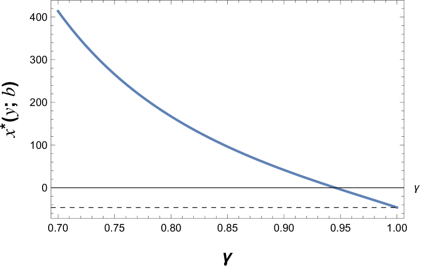
Figure 3. Values of $x^{*}(y;b)$ when varying $\gamma$ at $y=1$

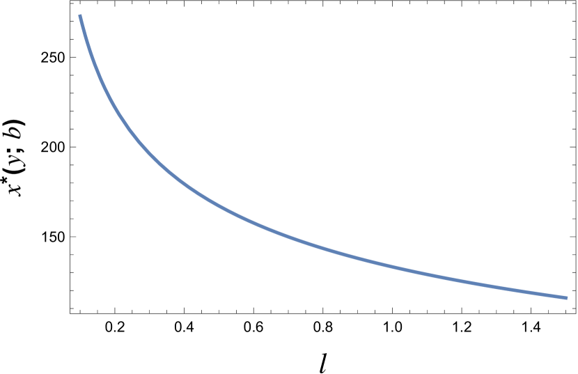
Figure 4. Values of $x^{*}(y;b)$ when varying $l$ at $y=1$

3.4.3. Optimal investment and consumption strategies

In this section, we illustrate the ratios of optimal strategies at time $0$ to initial wealth. Figure 6 shows a jump in the ratio of $\pi^{*}(x,y)/x$ in correspondence to the critical wealth level $x^{*}(y;b)$. Actually, this effect shares similarities to the so-called “saving for retirement”, where the optimal portfolio has a jump down at retirement (cf. [Dybvig and Liu, 2010]).

Figure 6 shows the ratio of optimal consumption at time $0$ to initial wealth. Interestingly, unlike the optimal investment strategy, the ratio of optimal consumption to wealth is smooth and there is no jump at the purchasing boundary because the marginal utility per unit of consumption does not change after buying life insurance.

Figure 5. Optimal portfolio feedback strategy at $y=1$

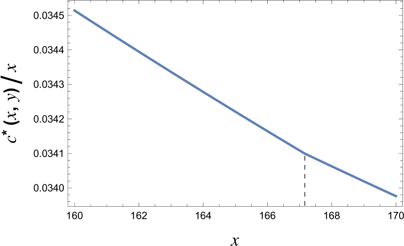
Figure 6. Optimal consumption feedback plan at $y=1$

4. A controlled bequest amount

4.1. Problem formulation

In this section, we assume the agent can choose how much money she plans to bequeath at death, i.e., $\{B_{t},t\geq 0\}$ is an $\mathcal{F}_{t}$-adapted control variable. Once purchased, the amount of bequest will be fixed. Correspondingly, when the agent chooses a target amount $B_{t}$ at purchasing time $t$, the premium $h_{t}$ in (2.2) is such that $h_{t}=mB_{t}$.

From (2.5), the agent’s wealth $X^{B}:=\{X^{c,\pi,B,\eta}_{t},t\geq 0\}$ now evolves as

(4.1) $$dX^{c,\pi,B,\eta}_{t}=[\pi_{t}(\mu-r)+rX^{c,\pi,B,\eta}_{t}-c_{t}-mB_{t}\mathds{1}_{\{t\geq\eta\}}+Y_{t}]dt+\pi_{t}\sigma dW_{t},\quad X_{0}^{c,\pi,B,\eta}=x.$$

In the following, we shall simply write $X^{B}$ to denote $X^{c,\pi,B,\eta}$, where needed. Then, the set of admissible strategies $\mathcal{A}^{B}(x,y)$ is as follows.

Definition 4.1.

Let $(x,y)\in\mathcal{O}$ be given and fixed. The triplet of choices $(c,\pi,B,\eta)$ is called an admissible strategy for $(x,y)$, and we write $(c,\pi,B,\eta)\in\mathcal{A}^{B}(x,y)$, if it satisfies the following conditions:

1. $c$ and $\pi$ are progressively measurable with respect to $\mathbb{F}$, $\eta\in\mathcal{S}$;

2. $c_{t}\geq 0$ for all $t\geq 0$ and $\int_{0}^{t}(c_{s}+|\pi_{s}|^{2})ds<\infty$ for all $t\geq 0$ $\ \mathbb{P}$-a.s.;

3. $B_{t}=0$ for all $0\leq t<\eta$ and $B_{t}=B_{\eta}\geq 0$ for any $t\geq\eta$, where $B_{\eta}$ is an $\mathcal{F}_{\eta}$-measurable random variable;

4. $X^{c,\pi,B,\eta}_{t}+g_{t}>\frac{mB_{t}}{r}\mathds{1}_{\{t\geq\eta\}}$ for all $t\geq 0$, where $g_{t}$ is defined in (2).

The term $\frac{mB_{t}}{r}:=\mathbb{E}[\int^{\infty}_{t}\frac{\xi_{s}}{\xi_{t}}mB_{t}ds|\mathcal{F}_{t}]$ in Condition (iv) is the present value of the future premium payment of the agent, under the assumption that the agent is always alive.

Similar to (3.1), and from (2) the agent aims at determining

$$V^{B}(x,y):=\sup_{(c,\pi,B,\eta)\in\mathcal{A}^{B}(x,y)}\mathbb{E}_{x,y}\bigg{[}\int^{\eta}_{0}e^{-(\rho+m)t}\Big{(}u(c_{t})+m\,u(0)\Big{)}dt$$

(4.2) $$+\int^{\infty}_{\eta}e^{-(\rho+m)t}\Big{(}u(c_{t})+m\,u(lB_{\eta})\Big{)}dt\bigg{]}.$$

In this section, we will focus on (4.1). Similar to Theorem 3.1, we also have the following immediate result.

Theorem 4.1.

When $\gamma>1$, the optimal purchasing time is $\eta^{*}=0$.

Hence, in the following, we focus on the case $0<\gamma<1$.

4.2. Solution to the problem for $\gamma\in(0,1)$

In this subsection, we determine the solution to (4.1) when $0<\gamma<1$, by employing a duality approach, which is analogous to the methods used in Section 3. First, we conduct successive transformations (cf. Subsections 4.2.1, 4.2.2 and 4.2.3) that connect the original stochastic control-stopping problem (with value function $V^{B}$) into its dual problem (with value function $v^{B}$). Then we study the reduced-version dual stopping problem (with value function $\widehat{v}^{B}$) and give our optimal purchasing time and optimal bequest amount of this section, see Theorem 4.4.

4.2.1. The static budget constraint

We now write down the static budget constraint by using the well-known method developed by [Karatzas et al., 1987] and [Cox and Huang, 1989]:

(4.3) $$\mathbb{E}_{x,y}\big{[}{\xi_{t}}X_{t}\big{]}+\mathbb{E}_{x,y}\bigg{[}\int_{0}^{t}\xi_{u}c_{u}du\bigg{]}\leq x+\mathbb{E}_{x,y}\bigg{[}\int_{0}^{t}\xi_{u}Y_{u}du\Bigg{]},\quad\text{if}\ 0\leq t\leq\eta,$$

and

(4.4) $$\mathbb{E}_{x,y}\big{[}{\xi_{t}}X_{t}\big{]}+\mathbb{E}_{x,y}\bigg{[}\int_{0}^{t}\xi_{u}\,\Big{(}c_{u}+mB_{0}\Big{)}\,du\bigg{]}\leq x+\mathbb{E}_{x,y}\bigg{[}\int_{0}^{t}\xi_{u}Y_{u}du\Bigg{]},\ \text{if}\ 0=\eta\leq t.$$

4.2.2. The optimization problem after purchasing life insurance

In this subsection, we shall look into the agent’s optimization problem after the purchase of life insurance. Apart from determining consumption and portfolio choices, the agent is also required to determine the optimal bequest amount $B^{*}_{\eta}$ at purchasing time $\eta$, where $\eta=0$ in this subsection.

Letting $\mathcal{A}^{B}_{0}(x,y):=\{(c,\pi,B):(c,\pi,B,0)\in\mathcal{A}^{B}(x,y)\},$ where the subscript $0$ indicates that the purchasing time $\eta$ is equal to $0$, the agent’s value function after purchasing life insurance then reads as

(4.5) $$\widehat{V}^{B}(x,y):=\sup_{(c,\pi,B)\in\mathcal{A}_{0}^{B}(x,y)}\mathbb{E}_{x,y}\bigg{[}\int^{\infty}_{0}e^{-(\rho+m)s}\Big{(}u(c_{s})+m\,u(lB_{0})\Big{)}ds\bigg{]}.$$

Recalling that $\xi_{s}=e^{-rs-\theta W_{s}-\frac{1}{2}\theta^{2}s}$, and for any pair $(c,\pi,B)\in\mathcal{A}_{0}^{B}(x,y)$ with a Lagrange multiplier $z>0$, we have

$$\mathbb{E}_{x,y}\bigg{[}\int_{0}^{\infty}e^{-(\rho+m)s}\Big{(}u(c_{s})+m\,u(lB_{0})\Big{)}ds\bigg{]}$$

$$\leq\mathbb{E}_{x,y}\bigg{[}\int_{0}^{\infty}e^{-(\rho+m)s}\Big{(}u(c_{s})+m\,u(lB_{0})\Big{)}ds\bigg{]}-z\mathbb{E}_{x,y}\bigg{[}\int_{0}^{\infty}\xi_{s}\Big{(}c_{s}+mB_{0}-Y_{s}\Big{)}ds\bigg{]}+zx$$

$$=\mathbb{E}_{x,y}\bigg{[}\int_{0}^{\infty}e^{-(\rho+m)s}\Big{(}u(c_{s})+m\,u(lB_{0})\Big{)}ds\bigg{]}$$

$$-\mathbb{E}_{x,y}\bigg{[}\int_{0}^{\infty}e^{-(\rho+m)s}zP_{s}\Big{(}c_{s}+mB_{0}-Y_{s}\Big{)}ds\bigg{]}+zx$$

$$=\mathbb{E}_{x,y}\bigg{[}\int_{0}^{\infty}e^{-(\rho+m)s}\bigg{(}u(c_{s})-zP_{s}c_{s}+zP_{s}Y_{s}\bigg{)}ds\bigg{]}$$

$$+\mathbb{E}_{x,y}\bigg{[}\int_{0}^{\infty}e^{-(\rho+m)s}\Big{(}m\,u(lB_{0})-zP_{s}mB_{0}\Big{)}ds\bigg{]}+zx$$

(4.6) $$\leq\mathbb{E}_{x,y}\bigg{[}\int_{0}^{\infty}e^{-(\rho+m)s}\Big{(}\widehat{u}(zP_{s})+zP_{s}Y_{s}\Big{)}ds\bigg{]}+zx+\bar{u}(z),$$

where the first inequality results from the budget constraint stated in (4.4), $P$ and $\widehat{u}$ are defined in (3.6), and

$$\quad\bar{u}(z) :=\sup_{B_{0}\geq 0}\mathbb{E}_{x,y}\bigg{[}\int_{0}^{\infty}e^{-(\rho+m)s}\Big{(}m\,u(lB_{0})-zP_{s}mB_{0}\Big{)}ds\bigg{]}$$

(4.7) $$=\sup_{B_{0}\geq 0}\Big{[}\frac{m\,u(lB_{0})}{\rho+m}-z\frac{mB_{0}}{r}\Big{]}=ml^{\frac{1-\gamma}{\gamma}}\frac{\gamma}{1-\gamma}r^{\frac{1-\gamma}{\gamma}}(\rho+m)^{-\frac{1}{\gamma}}z^{\frac{\gamma-1}{\gamma}},$$

with the optimizing bequest amount being

(4.8) $$B_{0}^{*}:=\Big{[}\frac{z(\rho+m)}{r}\Big{]}^{-\frac{1}{\gamma}}l^{\frac{1-\gamma}{\gamma}}.$$

Since the amount of bequest will be fixed once purchased, the (candidate) optimal bequest amount $B^{*}_{0}$ will just depend on the initial state $z$. This means the agent can choose the optimal bequest amount based on their initial state $z$ at the time of purchase ($\eta=0$ in this subsection).

Then we set

(4.9) $$\widehat{Q}^{B}(z,y):=\mathbb{E}_{z,y}\bigg{[}\int_{0}^{\infty}e^{-(\rho+m)s}\Big{[}\widehat{u}(Z_{s})+Z_{s}Y_{s}\Big{]}ds\bigg{]},$$

where $Z$ is given in (3.7).

Proposition 4.1.

One has $\widehat{Q}^{B}\in C^{2,2}(\mathbb{R}^{2}_{+}).$ Moreover, $\widehat{Q}^{B}$ satisfies

(4.10) $$-{\mathcal{L}}\widehat{Q}^{B}=\widehat{u}+zy,\ \text{on}\ \mathbb{R}^{2}_{+},$$

where $\mathcal{L}$ is defined in (3.10).

Proof.

The proof is given in A.7.

∎

It is possible to relate $\widehat{V}^{B}$ to $\widehat{Q}^{B}$ through the following duality relation.

Theorem 4.2.

The following dual relations hold:

$$\widehat{V}^{B}(x,y)=\inf_{z>0}[\widehat{Q}^{B}(z,y)+zx+\bar{u}(z)],\quad\widehat{Q}^{B}(z,y)=\sup_{x>-\frac{y}{\kappa}+\frac{mB_{0}}{r}}[\widehat{V}^{B}(x,y)-zx-\bar{u}(z)].$$

Proof.

Since $(c,\pi,B)\in\mathcal{A}^{B}_{0}(x,y)$ is arbitrary, taking the supremum over $(c,\pi,B)\in\mathcal{A}^{B}_{0}(x,y)$ on the left-hand side of (4.2.2) and recalling (4.5), we get, for any $z>0$,

$$\widehat{V}^{B}(x,y) \leq\mathbb{E}_{z,y}\bigg{[}\int_{0}^{\infty}e^{-(\rho+m)s}\Big{(}\widehat{u}(Z_{s})+Z_{s}Y_{s}\Big{)}ds\bigg{]}+zx+\bar{u}(z)$$

$$=\widehat{Q}^{B}(z,y)+zx+\bar{u}(z),$$

and thus

$$\widehat{Q}^{B}(z,y)\geq\sup_{x>\frac{mB_{0}}{r}-\frac{y}{\kappa}}[\widehat{V}^{B}(x,y)-zx-\bar{u}(z)]\quad\text{and}\quad\widehat{V}^{B}(x,y)\leq\inf_{z>0}[\widehat{Q}^{B}(z,y)+zx+\bar{u}(z)].$$

For the reverse inequalities, observe that the equality in (4.2.2) holds if and only if

(4.11) $$c_{s}=\mathcal{I}^{u}(Z_{s}),\quad B_{0}=\Big{[}\frac{z(\rho+m)}{r}\Big{]}^{-\frac{1}{\gamma}}l^{\frac{1-\gamma}{\gamma}}=:B^{*}_{0},$$

and

(4.12) $$\mathbb{E}_{x,y}\bigg{[}\int_{0}^{\infty}\xi_{s}\Big{(}c_{s}-Y_{s}+mB_{0}\Big{)}ds\bigg{]}=x,$$

where we denote by $\mathcal{I}^{u}$ the inverse of the marginal utility function $u_{c}(\cdot).$ Then, assuming (4.12) (we will prove its validity later), we define

$$\mathcal{X}^{B}(z,y) :=\mathbb{E}_{z,y}\bigg{[}\int_{0}^{\infty}\xi_{s}\Big{(}\mathcal{I}^{u}(Z_{s})-Y_{s}\Big{)}ds\bigg{]},$$

$$\mathcal{Y}^{B}(x,y) :=\mathbb{E}_{x,y}\bigg{[}\int_{0}^{\infty}e^{-(\rho+m)s}\Big{(}u(c_{s})+m\cdot u(lB_{0})\Big{)}ds\bigg{]},$$

and notice that (4.2.2), (4.11) and (4.12) yield

$$\mathcal{Y}^{B}\left(\mathcal{X}^{B}(z,y)+\frac{mB^{*}_{0}}{r},y\right)=\widehat{Q}^{B}(z,y)+z\left(\mathcal{X}^{B}(z,y)+\frac{mB_{0}^{*}}{r}\right)+\bar{u}(z)\leq\widehat{V}^{B}(x,y),$$

where the last inequality is due to $\mathcal{Y}^{B}(\mathcal{X}^{B}(z,y)+\frac{mB^{*}_{0}}{r},y)\leq\widehat{V}^{B}(x,y)$. The last display inequality thus provides

$$\widehat{Q}^{B}(z,y)\leq\sup_{x>\frac{mB_{0}}{r}-\frac{y}{\kappa}}[\widehat{V}^{B}(x,y)-zx-\bar{u}(z)]\quad\text{and}\quad\widehat{V}^{B}(x,y)\geq\inf_{z>0}[\widehat{Q}^{B}(z,y)+zx+\bar{u}(z)].$$

It thus remains only to show that equality (4.12) indeed holds. As a matter of fact, since $B^{*}_{0}$ is a constant, similar to Lemma A.1, we can prove the existence of a candidate optimal portfolio process $\pi^{*}$ such that $(c^{*},\pi^{*},B^{*})\in\mathcal{A}_{0}^{B}(x,y)$ and (4.12) holds, where $c_{s}^{*}=\mathcal{I}^{u}(Z_{s})$ is candidate optimal consumption process, $B^{*}_{0}=[\frac{z(\rho+m)}{r}]^{-\frac{1}{\gamma}}l^{\frac{1-\gamma}{\gamma}}$ is candidate optimal bequest process. By Theorem 3.6.3 in [Karatzas and Shreve, 1998b] or Lemma 6.2 in [Karatzas and Wang, 2000], one can then show that $(c^{*},\pi^{*},B^{*})$ is optimal for the problem $\widehat{V}^{B}$.

∎

4.2.3. The dual optimal stopping problem

Remember that we focus on $0<\gamma<1$ due to Theorem 4.1, that is $u(0)=0$. Now, for any $(x,y)\in\mathcal{O}$ and Lagrange multiplier $z>0$, from (4.1) and the budget constraint (4.3), recalling that $P_{s}$ as in (3.6), we have by the strong Markov property

$$\mathbb{E}_{x,y}\bigg{[}\int^{\eta}_{0}e^{-(\rho+m)t}u(c_{t})dt+\int^{\infty}_{\eta}e^{-(\rho+m)t}\Big{(}u(c_{t})+m\,u(lB_{\eta})\Big{)}dt\bigg{]}$$

$$\leq\sup_{(c,\pi,B,\eta)\in\mathcal{A}^{B}(x,y)}\mathbb{E}_{x,y}\bigg{[}\int^{\eta}_{0}e^{-(\rho+m)t}u(c_{t})dt+e^{-(\rho+m)\eta}\widehat{V}^{B}(X_{\eta},Y_{\eta})\bigg{]}$$

$$-z\mathbb{E}_{x,y}\bigg{[}\xi_{\eta}X_{\eta}+\int_{0}^{\eta}\xi_{t}\Big{(}c_{t}-Y_{t}\Big{)}dt\bigg{]}+zx$$

$$=\sup_{(c,\pi,B,\eta)\in\mathcal{A}^{B}(x,y)}\mathbb{E}_{x,y}\bigg{[}\int_{0}^{\eta}e^{-(\rho+m)s}\bigg{(}u(c_{s})-zP_{s}c_{s}+zP_{s}Y_{s}\bigg{)}ds$$

$$+e^{-(\rho+m)\eta}\widehat{V}^{B}(X_{\eta},Y_{\eta})-e^{-(\rho+m)\eta}zP_{\eta}X_{\eta}\bigg{]}+zx$$

$$\leq\sup_{\eta\in\mathcal{S}}\mathbb{E}_{z,y}\bigg{[}\int_{0}^{\eta}e^{-(\rho+m)s}\Big{(}\widehat{u}(Z_{s})+Z_{s}Y_{s}\Big{)}ds+e^{-(\rho+m)\eta}\Big{(}\widehat{Q}^{B}(Z_{\eta},Y_{\eta})+\bar{u}(Z_{\eta})\Big{)}\bigg{]}+zx,$$

where $\widehat{u}(z)=\sup_{c\geq 0}[u(c)-cz]$ and $Z_{t}$ is defined in (3.7).

Hence, setting

(4.13) $$v^{B}(z,y) :=\sup_{\eta\in\mathcal{S}}\mathbb{E}_{z,y}\bigg{[}\int_{0}^{\eta}e^{-(\rho+m)s}\Big{(}\widehat{u}(Z_{s})+Z_{s}Y_{s}\Big{)}ds+e^{-(\rho+m)\eta}\Big{(}\widehat{Q}^{B}(Z_{\eta},Y_{\eta})+\bar{u}(Z_{\eta})\Big{)}\bigg{]},$$

we have a two-dimensional optimal stopping problem, with dynamic $(Z,Y)$ as in (3.7) and (2.3).

In the following subsections, we study (4.13). Before doing that, similarly to Theorem 3.3, we have the following theorem that establishes a dual relation between the original problem (4.1) and the optimal stopping problem (4.13).

Theorem 4.3.

The following duality relations hold:

$$V^{B}(x,y)=\inf_{z>0}[v^{B}(z,y)+zx],\quad v^{B}(z,y)=\sup_{x>-\frac{y}{\kappa}}[V^{B}(x,y)-zx].$$

4.2.4. Study of the dual optimal stopping problem

To study the optimal stopping problem (4.13), it is convenient to introduce the function

(4.14) $$\widehat{v}^{B}(z,y):={v}^{B}(z,y)-{\widehat{Q}^{B}}(z,y)-\bar{u}(z).$$

Applying Itô’s formula to $\{e^{-(\rho+m)t}[\widehat{Q}^{B}(Z_{t},Y_{t})+\bar{u}(Z_{t})],t\in[0,\eta]\}$, and taking conditional expectations we have

$$\mathbb{E}_{z,y}\Big{[}e^{-(\rho+m)\eta}\Big{(}\widehat{Q}^{B}(Z_{\eta},Y_{\eta})+\bar{u}(Z_{\eta})\Big{)}\Big{]}=\widehat{Q}^{B}(z,y)+\bar{u}(z)$$

$$+\mathbb{E}_{z,y}\bigg{[}\int_{0}^{\eta}e^{-(\rho+m)s}\mathcal{L}\Big{(}\widehat{Q}^{B}(Z_{s},Y_{s})+\bar{u}(Z_{s})\Big{)}ds\bigg{]},$$

where $\mathcal{L}$ is defined in (3.10). Combining (4.13) and (4.14), we have

$$\widehat{v}^{B}(z,y) =\sup_{\eta\in\mathcal{S}}\mathbb{E}_{z,y}\bigg{[}\int_{0}^{\eta}e^{-(\rho+m)s}\Big{(}\widehat{u}(Z_{s})+Z_{s}Y_{s}\Big{)}ds+\int_{0}^{\eta}e^{-(\rho+m)s}\mathcal{L}\Big{(}\widehat{Q}^{B}(Z_{s},Y_{s})+\bar{u}(Z_{s})\Big{)}ds\bigg{]}$$

(4.15) $$=\sup_{\eta\in\mathcal{S}}\mathbb{E}_{z,y}\bigg{[}\int_{0}^{\eta}e^{-(\rho+m)s}\Big{(}-K\bar{u}(Z_{s})\Big{)}ds\bigg{]},$$

where $K:=\frac{1}{\gamma}(\rho+m-r(1-\gamma)-\frac{1-\gamma}{2\gamma}\theta^{2})>0$ due to Assumption 3.1, and where we have used the fact that (cf. (4.10))

$$\mathcal{L}(\widehat{Q}^{B}(z,y)+\bar{u}(z)) =-\widehat{u}(z)-zy-K\bar{u}(z).$$

From (4.2.4) we see that $\widehat{v}^{B}(z,y)$ is independent of $y$. Hence, it is the value of a one-dimensional optimal stopping problem, and in the following, with a slight abuse of notation, we simply write $\widehat{v}^{B}(z)$. As $\bar{u}>0$ when $0<\gamma<1$ (cf. (4.2.2)), the following result follows immediately (cf. also Theorem 4.1).

Theorem 4.4.

For any $\gamma\in(0,1)\cup(1,\infty)$, the optimal purchasing time is $\eta^{*}=0$; i.e., the agent should buy life insurance immediately. Moreover, the optimal bequest amount is $B^{*}_{0}=(\frac{z(\rho+m)}{r})^{-\frac{1}{\gamma}}l^{\frac{1-\gamma}{\gamma}}$.

Proof.

We know that when $0<\gamma<1$, $\widehat{v}^{B}(z)=\sup_{\eta\in\mathcal{S}}\mathbb{E}_{z}[\int_{0}^{\eta}e^{-(\rho+m)s}(-Kml^{\frac{1-\gamma}{\gamma}}\frac{\gamma}{1-\gamma}r^{\frac{1-\gamma}{\gamma}}(\rho+m)^{-\frac{1}{\gamma}}Z_{s}^{\frac{\gamma-1}{\gamma}})ds]=0$ (cf. (4.2.2) and (4.2.4)); hence $\widehat{v}^{B}(z)=0$ and $\eta^{*}=0$ a.s. for any $z\in\mathbb{R}_{+}$. Combining then Theorems 4.1 and (4.8), we conclude. ∎

4.3. Optimal strategies in terms of the primal variables

In the previous section, we studied the properties of the dual value function $v^{B}(z,y)$ and used $(z,y)$, where $z$ denotes the dual variable and $y$ denotes labour income, as the coordinate system for the study. In this section, we will come back to study of the value function $V^{B}(x,y)$ in the original coordinate system $(x,y)$, where $x$ denotes the wealth of the agent. Using arguments similar to those in Section 3.3, we give the explicit expressions of the value function and optimal policies in terms of the primal variables.

Theorem 4.5.

The value function $V^{B}$ in (4.1) is given by

$$V^{B}(x,y)=\frac{1}{\frac{1}{K}+m(lr)^{\frac{1-\gamma}{\gamma}}(\rho+m)^{-\frac{1}{\gamma}}}\frac{(\frac{y}{\kappa}+x)^{1-\gamma}}{1-\gamma}.$$

The optimal policies are ($c_{t}^{*},\pi_{t}^{*},B^{*}_{t},\eta^{*}$), with $c_{t}^{*}=c^{*}(X^{*}_{t},Y_{t}),\pi^{*}_{t}=\pi^{*}(X^{*}_{t},Y_{t})$, where

$$c^{*}(x,y) :=\frac{\frac{y}{\kappa}+x}{\frac{1}{K}+m(lr)^{\frac{1-\gamma}{\gamma}}(\rho+m)^{-\frac{1}{\gamma}}},$$

$$\pi^{*}(x,y) :=\bigg{(}\frac{\frac{y}{\kappa}+x}{\frac{1}{K}+m(lr)^{\frac{1-\gamma}{\gamma}}(\rho+m)^{-\frac{1}{\gamma}}}\bigg{)}\frac{\theta}{\gamma K\sigma}-\frac{\sigma_{y}y}{\kappa\sigma},$$

and

$$B^{*}_{0}(x,y):=\bigg{(}\frac{\frac{y}{\kappa}+x}{\frac{1}{K}+m(lr)^{\frac{1-\gamma}{\gamma}}(\rho+m)^{-\frac{1}{\gamma}}}\bigg{)}\bigg{(}\frac{\rho+m}{r}\bigg{)}^{-\frac{1}{\gamma}}l^{\frac{1-\gamma}{\gamma}}.$$

Furthermore, $\eta^{*}=0$ a.s. for any $(x,y)\in\mathcal{O}$ and the optimal wealth process is such that $X^{*}_{t}=\frac{(Z^{*}_{t})^{-\frac{1}{\gamma}}}{K}+\frac{mB^{*}_{0}}{r}-\frac{Y_{t}}{\kappa}$, where $Z_{t}^{*}$ is the solution to Equation (3.7) with the initial condition

$$Z_{0}^{*}=z^{*}(x,y):=\bigg{(}\frac{\frac{y}{\kappa}+x}{\frac{1}{K}+m(lr)^{\frac{1-\gamma}{\gamma}}(\rho+m)^{\frac{-1}{\gamma}}}\bigg{)}^{-\gamma}$$

and $x$ is the initial wealth at time $0$.

Proof.

The proof is given in Appendix A.8. ∎

4.4. Numerical illustrations

In this section, we provide numerical illustrations of the optimal strategies and of the value functions discussed in Theorem 4.5. Moreover, we investigate the sensitivities of the optimal bequest amount on relevant parameters and compare the differences between the predetermined case and the controlled case. The basic parameters are listed in Table 1.

4.4.1. Sensitivity analysis of optimal bequest amount

In this section, we study the sensitivity of the optimal bequest amount. Figure 8 shows that if $l$ is larger, the agent is more likely to buy more life insurance because the agent aligns more utility value on bequest. Figure 8 shows the effect of a change in $\gamma$ on the optimal bequest amount. If the risk aversion level $\gamma$ is larger, the agent with more risk aversion tends to buy more life insurance.

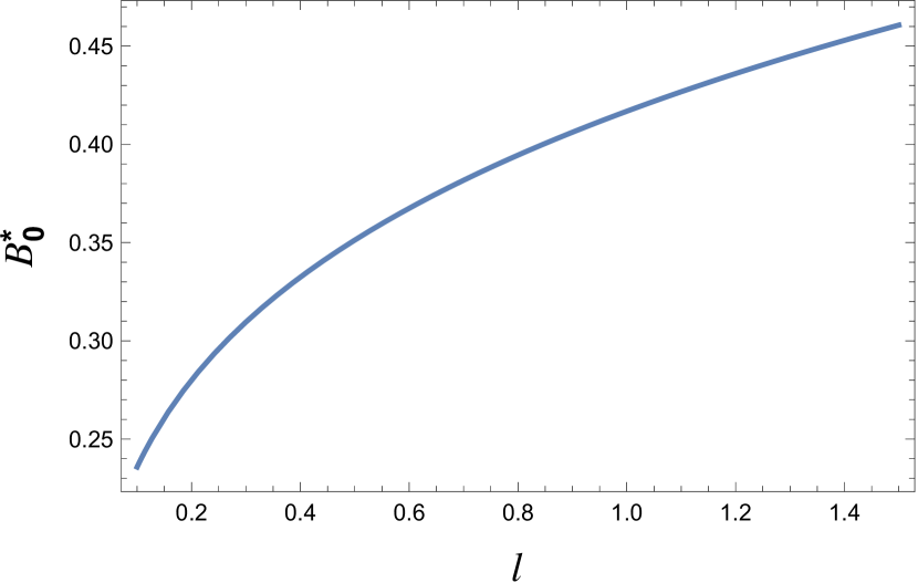
Figure 7. Values of $B^{*}_{0}$ when varying $l$ at $x=1,y=1$

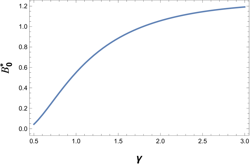
Figure 8. Values of $B^{*}_{0}$ when varying $\gamma$ at $x=1,y=1$

4.4.2. Comparison of optimal strategies and value functions

Here we compare the optimal strategies at initial time $0$ and value functions in both the predetermined bequest amount and the controlled bequest amount case, see Table 2. We find that when an agent whose initial wealth $x=1$ and predetermined bequest amount is $B=5$, the agent will invest more money than current wealth in risky asset because the future labor income is high. If we choose the predetermined bequest amount $B$ equal to the optimal bequest amount $B^{*}_{0}$ derived in the controlled case, then the optimal portfolio and optimal consumption plan are the same as that in the controlled case.

Table 2. Comparison of optimal strategies and value functions

Predetermined:	$x$	$B$	$\pi^{*}(x,y)/x$	$c^{*}(x,y)/x$	$\frac{y}{\kappa}$
Values:	1	5	33.482	1.477	55
Predetermined:	$x$	$B$	$\pi^{*}(x,y)/x$	$c^{*}(x,y)/x$
Values:	1	0.351	32.216	1.479
Controlled:	$x$	$B^{*}_{0}(x,y)/x$	$\pi^{*}(x,y)/x$	$c^{*}(x,y)/x$
Values:	1	0.351	32.216	1.479

5. Conclusions

This paper investigates the optimal timing of life insurance purchase for an agent facing uncertain lifetime and stochastic labor income. The agent can make a choice regarding when to buy life insurance, considering two types of bequests: One with a predetermined amount and the other granting the agent the freedom to determine the bequest amount as an additional variable. The optimization problem is formulated as a stochastic control-stopping problem over a random time horizon, which contains two state variables: Wealth and labor income. We have solved both cases using dual transformation and free-boundary approach, and obtained the analytical solutions for the value functions and optimal policies. We find there are different optimal life insurance purchasing strategies in the two cases and the risk aversion parameter $\gamma$ plays a crucial role. For example, when given a predetermined bequest amount, the agent should buy life insurance whenever her wealth exceeds a labor income-dependent optimal stopping boundary if $\gamma<1$, whereas life insurance should be bought immediately when $\gamma>1$. A detailed numerical study allows to draw interesting economic implications about the sensitivity of the optimal purchasing boundary and the optimal bequest amount with respect to the model’s parameters.

The paper offers several avenues for potential extensions. As discussed in Introduction, the study of the case with an age-dependent force of mortality will be a challenging research question. Additionally, exploring bequest as a luxury good could yield valuable insights. Moreover, incorporating the impact of health shocks in an individual’s optimization problem presents an interesting yet complex challenge due to life’s unpredictability and the potential for changing health status over time.

Appendix A Technical proofs and auxiliary results

A.1. Proof of Proposition 3.1

Proof.

First, we compute the convex dual of $u$ from (2.6) (cf. (3.6)); that is,

(A.1) $$\widehat{u}(z)=\frac{\gamma}{1-\gamma}z^{\frac{\gamma-1}{\gamma}},\quad z>0.$$

Therefore, by (3.8) and (A.1) we rewrite $\widehat{Q}(z,y)$ as follows

$$\widehat{Q}(z,y) =\mathbb{E}_{z,y}\bigg{[}\int_{0}^{\infty}e^{-(\rho+m)s}\frac{\gamma}{1-\gamma}{Z_{s}}^{\frac{\gamma-1}{\gamma}}ds\bigg{]}+\mathbb{E}_{z,y}\bigg{[}\int^{\infty}_{0}e^{-(\rho+m)s}Z_{s}Y_{s}ds\bigg{]}$$

$$+\mathbb{E}\bigg{[}\int_{0}^{\infty}e^{-(\rho+m)s}m\,u(lB)ds\bigg{]}$$

(A.2) $$=z^{\frac{\gamma-1}{\gamma}}\frac{\gamma}{1-\gamma}\int_{0}^{\infty}e^{-(\rho+m)s}e^{[\frac{\gamma-1}{\gamma}(\rho+m-r-\frac{1}{2}\theta^{2})+\frac{1}{2}\frac{(\gamma-1)^{2}\theta^{2}}{\gamma^{2}}]s}ds+\frac{zy}{\kappa}+\frac{m\,u(lB)}{\rho+m},$$

where we have used the explicit expression of $Z$. Moreover, due to Assumption 3.1 and (A.1), we can verify that

(A.3) $$\widehat{Q}(z,y)=z^{\frac{\gamma-1}{\gamma}}\frac{\gamma}{1-\gamma}\frac{1}{K}+\frac{zy}{\kappa}+\frac{m\,u(lB)}{\rho+m}<\infty,$$

where $K:=\frac{1}{\gamma}(\rho+m-r(1-\gamma)-\frac{1-\gamma}{2\gamma}\theta^{2})>0$ due to Assumption 3.1. Finally, it is easy to see that $\widehat{Q}\in C^{2,2}(\mathbb{R}^{2}_{+})$ from (A.3). Hence, it satisfies (3.9) by the well-known Feynman-Kac formula (see, e.g., Chapter 4 in [Karatzas and Shreve, 1998a]). ∎

A.2. Proof of Theorem 3.2

Proof.

Since $(c,\pi)\in\mathcal{A}_{0}(x,y)$ is arbitrary, taking the supremum over $(c,\pi)\in\mathcal{A}_{0}(x,y)$ on the left-hand side of (3.2.2) and recalling (3.4), we get, for any $z>0$,

$$\widehat{V}(x,y) \leq\mathbb{E}_{z,y}\bigg{[}\int_{0}^{\infty}e^{-(\rho+m)s}\Big{(}\widehat{u}(Z_{s})+Z_{s}Y_{s}+m\,u(lB)\Big{)}ds\bigg{]}+z(x-\frac{h}{r})$$

$$=\widehat{Q}(z,y)+z(x-\frac{h}{r}),$$

and thus

$$\widehat{Q}(z,y)\geq\sup_{x>\frac{h}{r}-\frac{y}{\kappa}}[\widehat{V}(x,y)-z(x-\frac{h}{r})]\quad\text{and}\quad\widehat{V}(x,y)\leq\inf_{z>0}[\widehat{Q}(z,y)+z(x-\frac{h}{r})].$$

For the reverse inequalities, observe that the equality in (3.2.2) holds if and only if

(A.4) $$c_{s}=\mathcal{I}^{u}(Z_{s}),$$

and

(A.5) $$\mathbb{E}_{x,y}\bigg{[}\int_{0}^{\infty}\xi_{s}\Big{(}c_{s}-Y_{s}\Big{)}ds\bigg{]}=x-\frac{h}{r},$$

where we denote by $\mathcal{I}^{u}$ the inverse of the marginal utility function $u_{c}(\cdot).$ Then, assuming (A.5) (we will prove its validity later), we define

$$\mathcal{X}(z,y):=\mathbb{E}_{z,y}\bigg{[}\int_{0}^{\infty}\xi_{s}\Big{(}\mathcal{I}^{u}(Z_{s})-Y_{s}\Big{)}ds\bigg{]},\quad\mathcal{Y}(x,y):=\mathbb{E}_{x,y}\bigg{[}\int_{0}^{\infty}e^{-(\rho+m)s}\Big{(}u(c_{s})+m\,u(lB)\Big{)}ds\bigg{]},$$

and notice that (3.2.2), (A.4) and (A.5) yield

$$\mathcal{Y}\left(\frac{h}{r}+\mathcal{X}(z,y),y\right)=\widehat{Q}(z,y)+z\mathcal{X}(z,y)\leq\widehat{V}(x,y),$$

where the last inequality is due to $\mathcal{Y}(\frac{h}{r}+\mathcal{X}(z,y),y)\leq\widehat{V}(x,y)$. The last display inequality thus provides

$$\widehat{Q}(z,y)\leq\sup_{x>\frac{h}{r}-\frac{y}{\kappa}}[\widehat{V}(x,y)-z(x-\frac{h}{r})]\quad\text{and}\quad\widehat{V}(x,y)\geq\inf_{z>0}[\widehat{Q}(z,y)+z(x-\frac{h}{r})].$$

It thus remains only to show that equality (A.5) indeed holds. As a matter of fact, Lemma A.1 guarantees the existence of a candidate optimal portfolio process $\pi^{*}$ such that $(c^{*},\pi^{*})\in\mathcal{A}_{0}(x,y)$ and (A.5) holds, where $c_{s}^{*}=\mathcal{I}^{u}(Z_{s})$ is candidate optimal consumption process. By Theorem 3.6.3 in [Karatzas and Shreve, 1998b] or Lemma 6.2 in [Karatzas and Wang, 2000], one can then show that $(c^{*},\pi^{*})$ is optimal for the problem $\widehat{V}$.

∎

A.3. Proof of Theorem 3.3

Proof.

Since $(c,\pi,\tau)\in\mathcal{A}(x,y)$ is arbitrary, taking the supremum over $(c,\pi,\tau)\in\mathcal{A}(x,y)$ on the left-hand side of (3.2.3), we get, for any $z>0,x>-\frac{y}{\kappa}$,

$${V}(x,y) \leq v(z,y)+zx,$$

so that $V(x,y)\leq\inf_{z>0}[v(z,y)+zx]$ and $v(z,y)\geq\sup_{x>-\frac{y}{\kappa}}[V(x,y)-zx]$.

For the inverse inequality, observe that equality holds in (3.2.3) if and only if

$$c_{s}=\mathcal{I}^{u}(Z_{s}),\quad\widehat{Q}(z,y)=\sup_{x>\frac{h}{r}-\frac{y}{\kappa}}[\widehat{V}(x,y)-z(x-\frac{h}{r})],$$

and

(A.6) $$\mathbb{E}_{x,y}\bigg{[}\xi_{\eta}X_{\eta}+\int_{0}^{\eta}\xi_{s}\Big{(}c_{s}-Y_{s}\Big{)}ds\bigg{]}=x,$$

where we recall that $\mathcal{I}^{u}$ denotes the inverse of the marginal utility function $u_{c}(\cdot).$ From Lemma A.2, we know that there exists a portfolio process $\pi^{*}$ such that (A.6) holds. From Theorem 3.2, we also know that $\widehat{Q}(z,y)=\sup_{x>\frac{h}{r}-\frac{y}{\kappa}}[\widehat{V}(x,y)-z(x-\frac{h}{r})]$.

Next we define

$$\bar{\mathcal{X}}(z,y):=\mathbb{E}_{z,y}\bigg{[}\int_{0}^{\eta}\xi_{s}\Big{(}\mathcal{I}^{u}(Z_{s})-Y_{s}\Big{)}ds\bigg{]},\quad\bar{\mathcal{Z}}(x,y):=\mathbb{E}_{x}[\xi_{\eta}X_{\eta}],$$

and

$$\bar{\mathcal{Y}}(x,y):=\mathbb{E}_{x,y}\bigg{[}\int_{0}^{\eta}e^{-(\rho+m)s}u(c_{s})ds+e^{-(\rho+m)\eta}\widehat{V}(X_{\eta},Y_{\eta})\bigg{]}.$$

Then by (3.2.3) and (A.6) we have

$$\bar{\mathcal{Y}}(\bar{\mathcal{X}}(z,y)+\bar{\mathcal{Z}}(x,y),y)=v(z,y)+z(\bar{\mathcal{X}}(z,y)+\bar{\mathcal{Z}}(x,y))\leq{V}(x,y),$$

where the last inequality is due to $\bar{\mathcal{Y}}(\bar{\mathcal{X}}(z,y)+\bar{\mathcal{Z}}(x,y),y)\leq{V}(x,y)$. This in turn gives

$$V(x,y)\geq\inf_{z>0}[v(z,y)+zx],\quad v(z,y)\leq\sup_{x>-\frac{y}{\kappa}}[V(x,y)-zx],$$

which completes the proof. ∎

A.4. Proof of Proposition 3.2

Proof.

From (3.13) and (3.14), it is clear that $\widehat{v}(z)\geq 0$ for all $z\in\mathbb{R}_{+}$. Moreover, from (3.2.4), we find that

$$\sup_{\eta\in\mathcal{S}}\mathbb{E}_{z}\bigg{[}\int^{\eta}_{0}Z_{t}hdt-\int^{\eta}_{0}e^{-(\rho+m)t}m\,u(lB)dt\bigg{]}$$

$$\leq\mathbb{E}_{z}\bigg{[}\int_{0}^{\infty}zhe^{-rt-\frac{1}{2}\theta^{2}t-\theta W_{t}}dt\bigg{]}=z\bigg{[}\int_{0}^{\infty}he^{-rt}dt\bigg{]}\leq\frac{zh}{r},$$

which implies the claim. ∎

A.5. Proof of Theorem 3.4

Proof.

The proof is organized in two steps.

Step 1: First we show that $\widehat{w}(z)$ in (3.21) satisfies the HJB equation (3.16). By construction, we only need to show that

(A.7) $$\Big{(}\mathbb{L}_{Z}-(\rho+m)\Big{)}\widehat{w}(z)+hz-m\,u(lB)\leq 0,\quad\forall z\leq b,$$

and

(A.8) $$\widehat{w}(z)\geq 0,\quad\forall z>b.$$

To prove (A.7), we define $F(z):=(\mathbb{L}_{Z}-(\rho+m))\widehat{w}(z)+hz-m\ u(lB)$, which is such that $F(z)=hz-m\,u(lB)$, since $\widehat{w}(z)=0$ when $z\leq b$. Therefore, $F^{\prime}(z)=h>0$ and $F(z)\leq 0$ for all $z\leq b$, due to $F(b)=0$. To prove (A.8), we notice that on $(b,\infty),\widehat{w}^{\prime\prime}(z)=\frac{-h(\alpha_{1}-1)}{r}\Big{(}\frac{m\,u(lB)r\alpha_{1}}{(\rho+m)h(\alpha_{1}-1)}\Big{)}^{1-\alpha_{1}}z^{\alpha_{1}-2}>0$ and $\widehat{w}^{\prime}(b)=0$, so that we have $\widehat{w}^{\prime}(z)\geq 0,z>b$. Since $\widehat{w}(b)=0$, it follows that $\widehat{w}(z)\geq 0$ for all $z>b$.

Step 2: We verify the optimality of $\widehat{w}(z)$ and of the stopping time $\eta(z;b)$ in (3.22). Note that $\widehat{w}$ in (3.21) is $C^{2}$ on $(0,b)\cup(b,\infty)$, but only $C^{1}$ at $b$. Let $z>0$ be given and fixed. We first show that $\widehat{w}(z)\geq\widehat{v}(z)$.

Applying Itô’s formula to the process $\{e^{-(\rho+m)t}\widehat{w}(Z_{t}),t\geq 0\}$, we find that

$$e^{-(\rho+m)t}\widehat{w}(Z_{t}) =\widehat{w}(z)+\int^{t}_{0}e^{-(\rho+m)s}\Big{(}\mathbb{L}_{Z}-(\rho+m)\Big{)}\widehat{w}(Z_{s})\mathds{1}_{\{Z_{s}\neq b\}}ds$$

(A.9) $$-\int^{t}_{0}e^{-(\rho+m)s}\theta Z_{s}\widehat{w}^{\prime}(Z_{s})dW_{s}.$$

The HJB equation (3.16) guarantees that $[\mathbb{L}_{Z}-(\rho+m)]\widehat{w}(z)\leq-hz+m\,u(lB)$ everywhere on $(0,\infty)$ but $b$. Since $\mathbb{P}_{z}(Z_{t}=b)=0$ for all $t$ and all $z$, we then obtain from (A.5) that

$$e^{-(\rho+m)t}\widehat{w}(Z_{t}) \leq\widehat{w}(z)+\int^{t}_{0}e^{-(\rho+m)s}\Big{(}-hZ_{s}+m\,u(lB)\Big{)}ds$$

(A.10) $$-\int^{t}_{0}e^{-(\rho+m)s}\theta Z_{s}\widehat{w}^{\prime}(Z_{s})dW_{s}.$$

Let $(\nu_{n})_{n\geq 1}$ be a localization sequence of (bounded) stopping times $(\nu_{n})_{n}$ diverging to infinity as $n\uparrow\infty$ for the continuous local martingale $\{\int^{t}_{0}e^{-(\rho+m)s}\theta Z_{s}\widehat{w}^{\prime}(Z_{s})dW_{s},t\geq 0\}$. Then for every stopping time $\eta$ of $Z$ we have by (A.5) above

$$e^{-(\rho+m)(\nu_{n}\wedge\eta)}\widehat{w}(Z_{\nu_{n}\wedge\eta}) \leq\widehat{w}(z)+\int^{\nu_{n}\wedge\eta}_{0}e^{-(\rho+m)s}\Big{(}-hZ_{s}+m\,u(lB)\Big{)}ds$$

$$-\int^{\nu_{n}\wedge\eta}_{0}e^{-(\rho+m)s}\theta Z_{s}\widehat{w}^{\prime}(Z_{s})dW_{s},$$

for all $n\geq 1$. Taking the $\mathbb{P}_{z}$-expectation, using the optional sampling theorem to conclude that $\mathbb{E}_{z}[\int^{\nu_{n}\wedge\eta}_{0}e^{-(\rho+m)s}\theta Z_{s}\widehat{w}^{\prime}(Z_{s})dW_{s}]=0$ for all $n$, and letting $n\to\infty$, we find by Fatou’s lemma that

(A.11) $$\widehat{w}(z)\geq\mathbb{E}_{z}[e^{-(\rho+m)\eta}\widehat{w}(Z_{\eta})]+\mathbb{E}_{z}\bigg{[}\int^{\eta}_{0}e^{-(\rho+m)s}(hZ_{s}-m\,u(lB))ds\bigg{]}.$$

Thus, by arbitrariness of $\eta\in\mathcal{S}$ and from (3.2.4), we find $\widehat{w}(z)\geq\widehat{v}(z)$ for all $z>0$.

Now consider the stopping time $\eta(z;b)$ defined in (3.22). We observe that the inequality in (A.5), therefore also in (A.11), becomes an equality. Moreover, $\widehat{w}(Z_{\eta(z;b)})=0$. Hence

$$\widehat{w}(z)=\mathbb{E}_{z}[e^{-(\rho+m)\eta(z;b)}\widehat{w}(Z_{\eta(z;b)})]+\mathbb{E}_{z}\bigg{[}\int^{\eta(z;b)}_{0}e^{-(\rho+m)s}\Big{(}hZ_{s}-m\,u(lB)\Big{)}ds\bigg{]}\leq\widehat{v}(z).$$

This shows that $\widehat{w}(z)=\widehat{v}(z)$ for all $z>0$ and $\eta(z;b)$ is optimal.

∎

A.6. Proof of Theorem 3.5

Proof.

The proof is organized in three steps.

Step 1: We start by giving explicit expressions of the value function in terms of the primal variables. Firstly, we compute $z^{*}(x,y)=\mathcal{I}^{v}(-x,y)$, where $\mathcal{I}^{v}(\cdot,y)$ is the inverse function of $v_{z}(\cdot,y)$. From (A.3), (3.14) and (3.21), we obtain

(A.12) $$v(z,y)=\left\{\begin{aligned} C_{1}z^{\alpha_{1}}+z^{\frac{\gamma-1}{\gamma}}\frac{\gamma}{(1-\gamma)K}+\frac{zy}{\kappa},\quad\text{if}\ &z>b,\\ z^{\frac{\gamma-1}{\gamma}}\frac{\gamma}{(1-\gamma)K}+\frac{yz}{\kappa}-\frac{hz}{r}+\frac{m\,u(lB)}{\rho+m},\quad\text{if}\ &0<z\leq b,\end{aligned}\right.$$

and

(A.13) $$v_{z}(z,y)=\left\{\begin{aligned} C_{1}\alpha_{1}z^{\alpha_{1}-1}-\frac{z^{-\frac{1}{\gamma}}}{K}+\frac{y}{\kappa},\quad\text{if}\ &z>b,\\ -\frac{z^{-\frac{1}{\gamma}}}{K}+\frac{y}{\kappa}-\frac{h}{r},\quad\text{if}\ &0<z\leq b.\end{aligned}\right.$$

Then from (A.13) we know

(A.14) $$z^{*}(x,y)=\Big{[}(x-\frac{h}{r}+\frac{y}{\kappa})K\Big{]}^{-\gamma},\quad\text{if}\ x\geq x^{*}(y;b),$$

and, if $-\frac{y}{\kappa}<x<x^{*}(y;b)$, $z^{*}{(x,y)}$ satisfies

(A.15) $$C_{1}\alpha_{1}(z^{*})^{\alpha_{1}-1}{(x,y)}-(z^{*})^{\frac{-1}{\gamma}}{(x,y)}\frac{1}{K}+\frac{y}{\kappa}+x=0.$$

From (3.23), (A.12) and (A.14) we thus find

$$V(x,y)=\left\{\begin{aligned} C_{1}(z^{*})^{\alpha_{1}}(x,y)+\frac{\gamma(z^{*})^{\frac{\gamma-1}{\gamma}}(x,y)}{(1-\gamma)K}+(\frac{y}{\kappa}+x)z^{*}(x,y),\quad\text{if}\ &-\frac{y}{\kappa}<x<x^{*}(y;b),\\ \frac{(x-\frac{h}{r}+\frac{y}{\kappa})^{1-\gamma}K^{-\gamma}}{1-\gamma}+\frac{m\,u(lB)}{\rho+m},\quad\text{if}\ &x\geq x^{*}(y;b),\end{aligned}\right.$$

where $z^{*}$ satisfies (A.15).

Step 2: We show that $V\in C^{2,2}(\mathcal{C})\cap C^{1,2}(\mathcal{O})$ and $V$ is a solution in the a.e. sense to the HJB equation

$$0=\max\Big{\{}\widehat{V}-V,\sup_{c,\pi}\Big{[}\frac{1}{2}\sigma^{2}\pi^{2}V_{xx}+\frac{1}{2}\sigma_{y}^{2}y^{2}V_{yy}+\mu_{y}yV_{y}+\sigma\pi\sigma_{y}yV_{xy}$$

(A.16) $$+(\pi(\mu-r)+rx-c+y)V_{x}+u(c)-(\rho+m)V\Big{]}\Big{\}}.$$

Step 2-(a): Firstly we show the regularity of $V$. From (3.23), using that $v_{z}(z^{*}(x,y),y)=-x$ and $v_{zy}(z^{*}(x,y),y)+v_{zz}(z^{*}(x,y),y)z_{y}^{*}(x,y)=0$ one has

$$V_{y}(x,y) =v_{y}(z^{*}(x,y),y)+v_{z}(z^{*}(x,y),y)z^{*}_{y}(x,y)+xz^{*}_{y}(x,y)=v_{y}(z^{*}(x,y),y),$$

$$V_{yy}(x,y) =v_{yy}(z^{*}(x,y),y)+v_{yz}(z^{*}(x,y),y)z^{*}_{y}(x,y),$$

$$V_{x}(x,y) =v_{z}(z^{*}(x,y),y)z^{*}_{x}(x,y)+z^{*}(x,y)+xz^{*}_{x}(x,y)=z^{*}(x,y),$$

$$V_{xy}(x,y) =z^{*}_{y}(x,y)=\frac{-v_{zy}(z^{*}(x,y),y)}{v_{zz}(z^{*}(x,y),y)},\ \text{in the a.e. sense},$$

(A.17) $$V_{xx}(x,y) =z_{x}^{*}(x,y)=-\frac{1}{v_{zz}(z^{*}(x,y),y)},\ \text{in the a.e. sense}.$$

Then we have $V\in C^{2,2}(\mathcal{C})\cap C^{1,2}(\mathcal{O})$ due to Corollary 3.1.

Step 2-(b): Now we show $V$ is a solution in the a.e. sense to the HJB equation (A.6). We define $\widetilde{Q}(z,y):=\widehat{Q}(z,y)-\frac{h}{r}z$. Recalling that $v\geq\widetilde{Q}$ on $\mathbb{R}^{2}_{+}$ by (3.13), we notice that if $v(z^{*}(x,y),y)=\widetilde{Q}(z^{*}(x,y),y)$, then the function $z\mapsto(v-\widetilde{Q})(z,y)$ attains its minimum value $0$ at $z^{*}(x,y).$ Hence,

$$v_{z}(z^{*}(x,y),y)=\widetilde{Q}_{z}(z^{*}(x,y),y)=-x.$$

This means that $z^{*}(x,y)$ is a stationary point of the convex function $z\mapsto\widetilde{Q}(z,y)+zx$, so that

$$\widetilde{Q}(z^{*}(x,y),y)+xz^{*}(x,y)=\min_{z}(\widetilde{Q}(z,y)+zx)=\min_{z}[\widehat{Q}(z,y)-\frac{h}{r}z+zx]=\widehat{V}(x,y),$$

by Theorem 3.2. Together with (3.23), we obtain $V(x,y)=\widehat{V}(x,y)$.

On the other hand, if $V(x,y)=\widehat{V}(x,y)$, then by (3.23) and Theorem 3.2,

$$v(z^{*}(x,y),y)+xz^{*}(x,y)=\inf_{z}(\widetilde{Q}(z,y)+zx)\leq\widetilde{Q}(z^{*}(x,y),y)+xz^{*}(x,y).$$

Hence, since $v\geq\widetilde{Q}$ on $\mathbb{R}^{2}_{+}$, $v(z^{*}(x,y),y)=\widetilde{Q}(z^{*}(x,y),y)$.

Combining these two arguments we have that

$$\{(x,y)\in\mathcal{O}:V(x,y)=\widehat{V}(x,y)\}=\{(x,y)\in\mathcal{O}:v(z^{*}(x,y),y)=\widetilde{Q}(z^{*}(x,y),y)\}.$$

This, together with (3.25), leads to express the optimal purchasing time in the original coordinates as

$$\left\{\begin{aligned} \eta^{*}(x,y)&=\inf\{t\geq 0:X^{x}_{t}\geq\widehat{b}(Y^{y}_{t})\}\\ &=\inf\{t\geq 0:V(X^{x}_{t},Y^{y}_{t})=\widehat{V}(X^{x}_{t},Y^{y}_{t})\}.\end{aligned}\right.$$

Due to the regularity of $V$ (cf. Step 2-(a)) and the dual relations between $V$ and $v$ (cf. (A.6)), from Corollary 3.1 we can deduce that $V$ is a solution in the a.e. sense to the HJB equation (A.6).

Step 3: Let $(x,y)\in\mathcal{O}$ and recall that $\mathcal{I}^{u}(\cdot)$ denotes the inverse of $u_{c}(\cdot)$. Then $c^{*}(x,y):=\mathcal{I}^{u}(V_{x}(x,y))$ and $\pi^{*}(x,y):=\frac{-\theta V_{x}(x,y)-\sigma_{y}yV_{xy}(x,y)}{\sigma V_{xx}(x,y)}$ (a.e. on $\mathcal{O}$) define the (candidate) optimal feedback maps, while $\eta^{*}(x,y)=\inf\{t\geq 0:V(X^{x}_{t},Y^{y}_{t})\leq\widehat{V}(X^{x}_{t},Y^{y}_{t})\}$ is the optimal purchasing time.

Next we give the explicit solutions for the (candidate) optimal policies. We set $x^{*}(y;b):=x^{*}(b,y),$ where $x^{*}(\cdot,y)$ is the inverse function of $z^{*}(\cdot,y).$ Since $v_{z}(z^{*}(x,y),y)=-x$, by taking $x=x^{*}(z,y)$, computations show that

$$v_{z}(z,y)=v_{z}(z^{*}(x^{*}(z,y),y),y)=-x^{*}(z,y).$$

Hence, from (3.24) and (A.13) we have

$$x^{*}(y;b) =x^{*}(b,y)=-v_{z}(b,y)=\frac{b^{-\frac{1}{\gamma}}}{K}-\frac{y}{\kappa}+\frac{h}{r},$$

where $b$ is given by (3.20).

To give the expression of optimal portfolio $\pi^{*}$, from (A.6) we deduce that

$$\pi^{*}(x,y)=\frac{-\theta V_{x}(x,y)-\sigma_{y}yV_{xy}(x,y)}{\sigma V_{xx}(x,y)}=\frac{\theta z^{*}(x,y)v_{zz}(z^{*}(x,y),y)-\sigma_{y}yv_{zy}(z^{*}(x,y),y)}{\sigma}.$$

By (A.13), direct calculations show that

$$v_{zz}(z,y)=\left\{\begin{aligned} C_{1}\alpha_{1}(\alpha_{1}-1)z^{\alpha_{1}-2}+\frac{z^{-\frac{1}{\gamma}-1}}{K\gamma},\quad\text{if}\ &z>b,\\ \frac{z^{-\frac{1}{\gamma}-1}}{K\gamma},\quad\text{if}\ &0<z\leq b,\end{aligned}\right.$$

and

$$v_{zy}(z,y)=\frac{1}{\kappa},\quad\text{for all}\ z>0.$$

Therefore, combining the above expressions we get

$$\pi^{*}(x,y)=\left\{\begin{aligned} \frac{\theta[C_{1}\alpha_{1}(\alpha_{1}-1)(z^{*})^{\alpha_{1}-1}(x,y)+\frac{(z^{*})^{-\frac{1}{\gamma}}(x,y)}{K\gamma}]-\frac{\sigma_{y}y}{\kappa}}{\sigma},\quad\text{if}\ &-\frac{y}{\kappa}<x<x^{*}(y;b),\\ \frac{\theta(x-\frac{h}{r}+\frac{y}{\kappa})\frac{1}{\gamma}-\frac{\sigma_{y}y}{\kappa}}{\sigma},\quad\text{if}\ &x\geq x^{*}(y;b),\end{aligned}\right.$$

where $z^{*}(x,y)$ is given in (A.15).

Then, we give the expression of optimal consumption $c^{*}$. Since $\mathcal{I}^{u}(x)=x^{-\frac{1}{\gamma}}$, we find

$$c^{*}(x,y)=\left\{\begin{aligned} (z^{*})^{-\frac{1}{\gamma}}(x,y),\quad\text{if}\ &-\frac{y}{\kappa}<x<x^{*}(y;b),\\ K(x+\frac{y}{\kappa}-\frac{h}{r}),\quad\text{if}\ &x\geq x^{*}(y;b),\end{aligned}\right.$$

where $z^{*}(x,y)$ is given in (A.15).

Let now $Z^{*}$ be a solution of SDE (3.7) with initial value $Z_{0}=z^{*}$. Similar to [Choi et al., 2008], in order to obtain the optimal wealth process we substitute $(Z_{t}^{*},Y_{t})$ for $(z^{*},y)$ into (A.14) and (A.15), respectively. Then for $X_{t}\geq\widehat{b}(Y_{t})$, we have

(A.18) $$X^{*}_{t}=\frac{(Z^{*}_{t})^{-\frac{1}{\gamma}}}{K}+\frac{h}{r}-\frac{Y_{t}}{\kappa}.$$

Applying Itô’s formula to (A.18), we have

$$dX_{t}^{*}=[\pi^{*}_{t}(\mu-r)+rX^{*}_{t}-c^{*}_{t}-h_{t}+Y_{t}]dt+\pi_{t}^{*}\sigma dW_{t}.$$

So the optimal wealth is induced by the strategies $(c^{*},\pi^{*})$ for $X_{t}\geq\widehat{b}(Y_{t})$. Similarly, for $-\frac{Y_{t}}{\kappa}<X_{t}<\widehat{b}(Y_{t})$, we have

(A.19) $$X^{*}_{t}=-C_{1}\alpha_{1}(Z^{*}_{t})^{\alpha_{1}-1}+\frac{(Z^{*}_{t})^{-\frac{1}{\gamma}}}{K}-\frac{Y_{t}}{\kappa},$$

and we also obtain

$$dX_{t}^{*}=[\pi^{*}_{t}(\mu-r)+rX^{*}_{t}-c^{*}_{t}+Y_{t}]dt+\pi_{t}^{*}\sigma dW_{t}.$$

Hence, the optimal wealth is indeed induced by the strategies $(c^{*},\pi^{*})$ for $-\frac{Y_{t}}{\kappa}<X_{t}<\widehat{b}(Y_{t})$ as well. Moreover, by (A.18) and (A.19), we can verify that that $X^{*}_{t}$ satisfies the borrowing constraint in Definition 3.1.

Finally, by a standard verification argument we know that $c^{*}_{t}=c^{*}(X^{*}_{t},Y_{t}),\pi^{*}_{t}=\pi^{*}(X^{*}_{t},Y_{t})$ and $\eta^{*},\mathbb{P}_{x,y}$-a.s., provide an optimal control triple. ∎

A.7. Proof of Proposition 4.1

Proof.

By (A.1) and (4.9) we rewrite $\widehat{Q}^{B}(z,y)$ as follows

$$\widehat{Q}^{B}(z,y) =\mathbb{E}_{z,y}\bigg{[}\int_{0}^{\infty}e^{-(\rho+m)s}\frac{\gamma}{1-\gamma}{Z_{s}}^{\frac{\gamma-1}{\gamma}}ds\bigg{]}+\mathbb{E}_{z,y}\bigg{[}\int^{\infty}_{0}e^{-(\rho+m)s}Z_{s}Y_{s}ds\bigg{]}$$

(A.20) $$=z^{\frac{\gamma-1}{\gamma}}\frac{\gamma}{1-\gamma}\int_{0}^{\infty}e^{-(\rho+m)s}e^{[\frac{\gamma-1}{\gamma}(\rho+m-r-\frac{1}{2}\theta^{2})+\frac{1}{2}\frac{(\gamma-1)^{2}\theta^{2}}{\gamma^{2}}]s}ds+\frac{zy}{\kappa},$$

where we have used the explicit expression of $Z$. Moreover, due to Assumption 3.1 and (A.7), we can verify that

(A.21) $$\widehat{Q}^{B}(z,y)=z^{\frac{\gamma-1}{\gamma}}\frac{\gamma}{1-\gamma}\frac{1}{K}+\frac{zy}{\kappa}<\infty,$$

where $K=\frac{1}{\gamma}(\rho+m-r(1-\gamma)-\frac{1-\gamma}{2\gamma}\theta^{2})>0$ due to Assumption 3.1. Finally, it is easy to see that $\widehat{Q}^{B}\in C^{2,2}(\mathbb{R}^{2}_{+})$ from (A.21). Hence, it satisfies (4.10) by the well-known Feynman-Kac formula (see, e.g., Chapter 4 in [Karatzas and Shreve, 1998a]). ∎

A.8. Proof of Theorem 4.5

Proof.

The proof is organized in three steps.

Step 1: From Theorem 4.4, we know that $\eta^{*}=0$. It means that $V^{B}(x,y)=\widehat{V}^{B}(x,y)$. For any $(x,y)\in\mathcal{O}$, we have that $\widehat{V}^{B}(x,y)=\inf_{z>0}[\widehat{Q}^{B}(z,y)+zx+\bar{u}(z)]$ by Theorem 4.2. Moreover, it is easy to check that $\widehat{Q}^{B}(z,y)+\bar{u}(z)$ is strictly convex with respect to $z$ (cf. (A.21)). Then there exists a unique solution $z^{*}(x,y)>0$ such that

(A.22) $$\widehat{V}^{B}(x,y)=\widehat{Q}^{B}(z^{*}(x,y),y)+z^{*}(x,y)x+\bar{u}(z^{*}(x,y)),$$

where $z^{*}(x,y):=\mathcal{I}^{Q}(-x,y)$ and $\mathcal{I}^{Q}(\cdot,y)$ is the inverse function of $(\widehat{Q}^{B}_{z}+\bar{u}_{z})(\cdot,y)$. Moreover, $z^{*}\in C(\mathcal{O}),$ and $z^{*}(x,y)$ is strictly decreasing with respect to $x$, which is a bijection form. Hence, for any $y\in\mathbb{R}_{+}$, $z^{*}(\cdot,y)$ has an inverse function $x^{*}(\cdot,y)$, which is continuous, strictly decreasing, and maps $\mathbb{R}_{+}$ to $(-\frac{y}{\kappa},\infty)$.

Step 2: We now give explicit expressions of the value function in terms of the primal variables. Firstly, we compute $z^{*}(x,y)=\mathcal{I}^{Q}(-x,y)$. From (4.2.2) and (A.21), we obtain

$$\widehat{Q}^{B}_{z}(z,y)=-z^{-\frac{1}{\gamma}}\frac{1}{K}+\frac{y}{\kappa},\quad\bar{u}_{z}(z)=-ml^{\frac{1-\gamma}{\gamma}}r^{\frac{1-\gamma}{\gamma}}(\rho+m)^{-\frac{1}{\gamma}}z^{-\frac{1}{\gamma}},$$

and

(A.23) $$z^{*}(x,y)=\bigg{[}\frac{\frac{y}{\kappa}+x}{\frac{1}{K}+m(lr)^{\frac{1-\gamma}{\gamma}}(\rho+m)^{\frac{-1}{\gamma}}}\bigg{]}^{-\gamma}.$$

From (A.21), (A.22) and (A.23), we thus find

$${V}^{B}(x,y)=\widehat{V}^{B}(x,y)=\frac{1}{\frac{1}{K}+m(lr)^{\frac{1-\gamma}{\gamma}}(\rho+m)^{-\frac{1}{\gamma}}}\frac{(\frac{y}{\kappa}+x)^{1-\gamma}}{1-\gamma}.$$

Step 3: Here we show the optimal policies. Let $Z^{*}$ be a solution of SDE (3.7) with initial value $Z_{0}=z^{*}$, where $z^{*}$ is given in (A.23). From Theorem 4.2, we already know that the existence of a candidate optimal portfolio process $\pi^{*}$ such that $(c^{*},\pi^{*},B^{*})\in\mathcal{A}_{0}^{B}(x,y)$ and (4.12) holds, where $c_{s}^{*}=\mathcal{I}^{u}(Z_{s})$ is the candidate optimal consumption process, $B^{*}_{0}=[\frac{z(\rho+m)}{r}]^{-\frac{1}{\gamma}}l^{\frac{1-\gamma}{\gamma}}$ is the candidate optimal bequest. Moreover, by Theorem 3.6.3 in [Karatzas and Shreve, 1998b] or Lemma 6.2 in [Karatzas and Wang, 2000], one can then show that $(c^{*},\pi^{*},B^{*})$ is optimal for the problem $\widehat{V}^{B}$. It thus remains only to find the expressions of optimal portfolio $\pi^{*}$.

In fact, from (4.12) we have

(A.24) $$X_{t}^{*}=\frac{1}{\xi_{t}}\mathbb{E}_{x,y}\bigg{[}\int^{\infty}_{t}\xi_{s}(c_{s}+mB_{0}-Y_{s})\bigg{|}\mathcal{F}_{t}\bigg{]}=\frac{(Z^{*}_{t})^{-\frac{1}{\gamma}}}{K}+\frac{mB_{0}^{*}}{r}-\frac{Y_{t}}{\kappa}.$$

Applying Itô’s formula to (A.24), we have

$$dX_{t}^{*}=\bigg{[}\frac{Z_{t}^{-\frac{1}{\gamma}}}{K}\Big{(}-\frac{1}{\gamma}(\rho-r+m)+(\frac{1+\gamma}{2\gamma^{2}})\theta^{2}\Big{)}-\frac{\mu_{y}Y_{t}}{\kappa}\bigg{]}dt+\bigg{[}Z_{t}^{-\frac{1}{\gamma}}\frac{\theta}{K\gamma}-\frac{\sigma_{y}Y_{t}}{\kappa}\bigg{]}dW_{t}.$$

Then comparing $X^{*}$ above with (4.1), we can find that

(A.25) $$\pi^{*}_{t}=\frac{\theta(Z_{t}^{*})^{-\frac{1}{\gamma}}}{\gamma K\sigma}-\frac{\sigma_{y}Y_{t}}{\kappa\sigma},$$

and the optimal wealth is indeed induced by the strategies $(c^{*},\pi^{*},B^{*}).$

Finally, we give the explicit solutions for the optimal polices. From (A.23) and (A.25) we deduce that

$$\pi^{*}(x,y)=\frac{\theta(z^{*})^{-\frac{1}{\gamma}}}{\gamma K\sigma}-\frac{\sigma_{y}y}{\kappa\sigma}=\bigg{[}\frac{\frac{y}{\kappa}+x}{\frac{1}{K}+m(lr)^{\frac{1-\gamma}{\gamma}}(\rho+m)^{\frac{-1}{\gamma}}}\bigg{]}\frac{\theta}{\gamma K\sigma}-\frac{\sigma_{y}y}{\kappa\sigma}.$$

Since $\mathcal{I}^{u}(x)=x^{-\frac{1}{\gamma}}$, then we have

$$c^{*}(x,y)=\mathcal{I}^{u}(z^{*})=\bigg{[}\frac{\frac{y}{\kappa}+x}{\frac{1}{K}+m(lr)^{\frac{1-\gamma}{\gamma}}(\rho+m)^{\frac{-1}{\gamma}}}\bigg{]}.$$

Moreover, the optimal bequest amount is given by

$$B^{*}_{0}=\Big{[}\frac{z^{*}(\rho+m)}{r}\Big{]}^{-\frac{1}{\gamma}}l^{\frac{1-\gamma}{\gamma}}=\bigg{[}\frac{\frac{y}{\kappa}+x}{\frac{1}{K}+m(lr)^{\frac{1-\gamma}{\gamma}}(\rho+m)^{\frac{-1}{\gamma}}}\bigg{]}\Big{[}\frac{\rho+m}{r}\Big{]}^{-\frac{1}{\gamma}}l^{\frac{1-\gamma}{\gamma}}.$$

∎

A.9. Some auxiliary results

Lemma A.1.

Let $x+g_{0}>\frac{h}{r}$ be given, let $c\geq 0$ be a consumption process satisfying

$$\mathbb{E}_{x,y}\bigg{[}\int_{0}^{\infty}\xi_{s}c_{s}ds\bigg{]}=x+g_{0}-\frac{h}{r}.$$

Then, there exists a portfolio process $\pi$ such that the pair $(c,\pi)$ is admissible and

$$X^{c,\pi,\tau}_{s}+g_{s}>\frac{h}{r},\ \text{for}\ s\geq\eta.$$

Proof.

Let us define $L_{s}:=\int^{s}_{0}\xi_{u}c_{u}du$ and consider the nonnegative martingale

$$M_{s}:=\mathbb{E}[L_{\infty}|\mathcal{F}_{s}],\ s\geq 0.$$

According to the martingale representation theorem, there is an $\mathbb{F}$-adapted process $\phi$ satisfying $\int^{\infty}_{0}||\phi_{u}||^{2}du<\infty$ almost surely and

$$M_{s}=M_{0}+\int^{s}_{0}\phi_{u}dW_{u}=x+g_{0}-\frac{h}{r}+\int^{s}_{0}\phi_{u}dW_{u},\ s\geq 0.$$

Define then the nonnegative process $X$ by

$$X_{s} :=\frac{1}{\xi_{s}}\mathbb{E}\bigg{[}\int^{\infty}_{s}\xi_{u}c_{u}du\bigg{|}\mathcal{F}_{s}\bigg{]}+\frac{h}{r}-g_{s}=\frac{1}{\xi_{s}}[M_{s}-L_{s}]+\frac{h}{r}-g_{s},$$

so that $X_{0}=x,M_{0}=x-\frac{h}{r}+g_{0}.$ Itô’s rule implies

$$d(e^{-rs}X_{s})=-c_{s}e^{-rs}ds-he^{-rs}ds+Y_{s}e^{-rs}ds+e^{-rs}\pi_{s}\sigma dW_{s},$$

where $\pi_{s}:=\frac{1}{\xi_{s}\sigma}[\phi_{s}+(M_{s}-L_{s})\theta]$. It is easy to check that $\pi$ satisfies $\int^{\infty}_{0}|\pi_{s}|^{2}ds<\infty$ a.s. (see, e.g., Theorem 3.3.5 in [Karatzas and Shreve, 1998b]). We thus conclude that $X_{s}=X^{c,\pi,\tau}_{s}$ when $s\geq\eta$, by comparison with (2.5). Finally, since $X_{s}+g_{s}>\frac{h}{r}$ for $s\geq\eta$, the pair $(c,\pi)$ is admissible, and $X^{c,\pi,\tau}_{s}+g_{s}>\frac{h}{r},\ \text{for}\ s\geq\eta.$

∎

Lemma A.2.

For any $\eta\in\mathcal{S}$, let $x+g_{0}>0$ be given, let $c\geq 0$ be a consumption process. For any $\mathcal{F}_{\eta}$-measurable random variable $\phi$ with $\mathbb{P}[\phi>-g_{\eta}]=1$ such that

$$\mathbb{E}_{x,y}\bigg{[}\xi_{\eta}\phi+\int_{0}^{\eta}\xi_{s}c_{s}ds\bigg{]}=x+g_{0},$$

there exists a portfolio process $\pi$ such that the pair $(c,\pi)$ is admissible and

$$X^{c,\pi,\eta}_{s}+g_{s}>0,\ \text{for}\ s\leq\eta,\ \phi=X^{c,\pi,\eta}_{\eta}.$$

Proof.

The proof is similar to Lemma 6.3 in [Karatzas and Wang, 2000], and we thus omit details.

∎

References

- [Bayraktar and Young, 2013] Bayraktar, E. and Young, V. R. (2013). Life insurance purchasing to maximize utility of household consumption. North American Actuarial Journal, 17(2):114–135.
- [Braun et al., 2016] Braun, A., Schmeiser, H., and Schreiber, F. (2016). On consumer preferences and the willingness to pay for term life insurance. European Journal of Operational Research, 253(3):761–776.
- [Campbell, 1980] Campbell, R. A. (1980). The demand for life insurance: An application of the economics of uncertainty. The Journal of Finance, 35(5):1155–1172.
- [Chen et al., 2021] Chen, A., Hentschel, F., and Steffensen, M. (2021). On retirement time decision making. Insurance: Mathematics and Economics, 100:107–129.
- [Chen et al., 2022] Chen, C.-C., Chang, C.-C., Sun, E. W., and Yu, M.-T. (2022). Optimal decision of dynamic wealth allocation with life insurance for mitigating health risk under market incompleteness. European Journal of Operational Research, 300(2):727–742.
- [Choi and Shim, 2006] Choi, K. J. and Shim, G. (2006). Disutility, optimal retirement, and portfolio selection. Mathematical Finance, 16(2):443–467.
- [Choi et al., 2008] Choi, K. J., Shim, G., and Shin, Y. H. (2008). Optimal portfolio, consumption-leisure and retirement choice problem with CES utility. Mathematical Finance, 18(3):445–472.
- [Cox and Huang, 1989] Cox, J. C. and Huang, C.-f. (1989). Optimal consumption and portfolio policies when asset prices follow a diffusion process. Journal of Economic Theory, 49(1):33–83.
- [Dybvig and Liu, 2010] Dybvig, P. H. and Liu, H. (2010). Lifetime consumption and investment: retirement and constrained borrowing. Journal of Economic Theory, 145(3):885–907.
- [Farhi and Panageas, 2007] Farhi, E. and Panageas, S. (2007). Saving and investing for early retirement: A theoretical analysis. Journal of Financial Economics, 83(1):87–121.
- [Ferrari and Zhu, 2023] Ferrari, G. and Zhu, S. (2023). Optimal retirement choice under age-dependent force of mortality. arXiv preprint arXiv:2311.12169.
- [Huang and Milevsky, 2008] Huang, H. and Milevsky, M. A. (2008). Portfolio choice and mortality-contingent claims: The general HARA case. Journal of Banking & Finance, 32(11):2444–2452.
- [Karatzas and Kou, 1998] Karatzas, I. and Kou, S. G. (1998). Hedging American contingent claims with constrained portfolios. Finance and Stochastics, 2(3):215–258.
- [Karatzas et al., 1986] Karatzas, I., Lehoczky, J. P., Sethi, S. P., and Shreve, S. E. (1986). Explicit solution of a general consumption/investment problem. Mathematics of Operations Research, 11(2):261–294.
- [Karatzas et al., 1987] Karatzas, I., Lehoczky, J. P., and Shreve, S. E. (1987). Optimal portfolio and consumption decisions for a “small investor” on a finite horizon. SIAM Journal on Control and Optimization, 25(6):1557–1586.
- [Karatzas and Shreve, 1998a] Karatzas, I. and Shreve, S. (1998a). Brownian motion and stochastic calculus, volume 113. Springer Science & Business Media.
- [Karatzas and Shreve, 1998b] Karatzas, I. and Shreve, S. E. (1998b). Methods of mathematical finance, volume 39. Springer.
- [Karatzas and Wang, 2000] Karatzas, I. and Wang, H. (2000). Utility maximization with discretionary stopping. SIAM Journal on Control and Optimization, 39(1):306–329.
- [Li et al., 2007] Li, D., Moshirian, F., Nguyen, P., and Wee, T. (2007). The demand for life insurance in OECD countries. Journal of Risk and Insurance, 74(3):637–652.
- [Merton, 1971] Merton, R. C. (1971). Optimum consumption and portfolio rules in a continuous-time model. volume 3, pages 373–413. Elsevier.
- [Park et al., 2023] Park, K., Wong, H. Y., and Yan, T. (2023). Robust retirement and life insurance with inflation risk and model ambiguity. Insurance: Mathematics and Economics, 110:1–30.
- [Peskir and Shiryaev, 2006] Peskir, G. and Shiryaev, A. (2006). Optimal stopping and free-boundary problems. Springer.
- [Pliska and Ye, 2007] Pliska, S. R. and Ye, J. (2007). Optimal life insurance purchase and consumption/investment under uncertain lifetime. Journal of Banking & Finance, 31(5):1307–1319.
- [Richard, 1975] Richard, S. F. (1975). Optimal consumption, portfolio and life insurance rules for an uncertain lived individual in a continuous time model. Journal of Financial Economics, 2(2):187–203.
- [Wei et al., 2020] Wei, J., Cheng, X., Jin, Z., and Wang, H. (2020). Optimal consumption–investment and life-insurance purchase strategy for couples with correlated lifetimes. Insurance: Mathematics and Economics, 91:244–256.