From Augmentation to Decomposition: A New Look at CUPED in 2023
Abstract
Ten years ago, CUPED (Controlled Experiments Utilizing Pre-Experiment Data) (Deng et al., 2013) mainstreamed the idea of variance reduction leveraging pre-experiment covariates. Since its introduction, it has been implemented, extended, and modernized by major online experimentation platforms (Xie and Aurisset, 2016; Guo et al., 2021; Poyarkov et al., 2016; Jin and Ba, 2023; Cosgrove et al., 2022). Many researchers and practitioners often interpret CUPED as a regression adjustment (Lin, 2013; Tsiatis et al., 2008). In this article, we clarify its similarities and differences to regression adjustment and present CUPED as a more general augmentation framework which is closer to the spirit of the 2013 paper. We show that the augmentation view naturally leads to cleaner developments of variance reduction beyond simple average metrics, including ratio metrics and percentile metrics. Moreover, the augmentation view can go beyond using pre-experiment data and leverage in-experiment data, leading to significantly larger variance reduction. We further introduce metric decomposition using approximate null augmentation (ANA) as a mental model for in-experiment variance reduction. We study it under both a Bayesian framework and a frequentist optimal proxy metric framework. Metric decomposition arises naturally in conversion funnels, so this work has broad applicability.
1 Introduction
The CUPED method proposed by Deng et al. (2013) was inspired by the method of control variates from stochastic simulation (Asmussen and Glynn, 2008; Owen, 2013). CUPED is a model-free method that relies only on the observation that any pre-experiment difference between two randomized groups is pure noise due to randomization and should be in expectation. The model-free aspect is at the heart of CUPED; there is no assumption of a relationship of any form between the covariates and the target metric, as long as they have a nonzero correlation to exploit. Also, the authors developed the theory directly on estimators (of metrics and ’s), instead of modeling individual subject-level data points like regression models do. However, many blogs and papers citing CUPED often interpret it as a regression adjustment method, focusing on defining it in terms of averages of individual residuals.
2023 marks a decade since CUPED’s initial publication. In this work, we present CUPED as an augmentation framework which is closer to the spirit of the in initial proposal in the 2013 paper. We show that the augmentation view naturally leads to variance reduction beyond simple average metrics; it easily handles ratio metrics and percentile metrics as well. Moreover, the augmentation view can go beyond using pre-experiment data and leverage in-experiment data, leading to significantly larger variance reduction. We further introduce metric decomposition as a mental model for in-experiment variance reduction and present a Bayesian variance reduction framework. Metric decomposition arises naturally in conversion funnels, so this work has broad applicability.
Notation
Henceforth, we denote the observed metric value from the treatment and control groups as and , the unknown true average treatment effect (ATE) as , and we use to denote the naive estimate of based on the difference between two metric values. This is also denoted as .
2 CUPED as Augmentation
2.1 Three Simple Insights that Underlie CUPED
First insight: Augmentation with Mean-Zero Term
For any estimator of , define a new estimator
| (1) |
such that . Then is also an estimator of and is unbiased if is. Thus, the CUPED estimator is a mean-preserving augmentation of any existing estimator. The purpose of the augmentation is to find an augmentation such that
Second Insight: Optimal Variance Reduction from a Linear Family
The second insight of CUPED is that variance reduction is almost guaranteed with any mean-zero augmentation ! This is because any mean-zero augmentation can be multiplied by a scalar yielding a whole family of mean-zero augmentations , with variance . This variance is minimized when
with minimum variance
The amount of variance reduction from augmentation by is equal to the correlation between the augmentation term and the existing estimator . Any mean-zero augmentation is like a direction of gradient descent, and variance is optimally reduced with an appropriate choice of step size.
Third Insight: Existence of Mean-Zero Augmentation
The final insight of CUPED is that mean-zero augmentations are abundant if we tap into pre-experiment period data. Let be any metric computed from a (multivariate) signal on pre-experiment period data (e.g., or a percentile, etc.). Then is a mean-zero augmentation.
2.2 Relation to Regression Adjustment
When the metric of interest is a simple average and the naive estimator of ATE is the difference in means , and the augmentation is also a difference in means , CUPED is often compared to regression adjustment of the form
| (ANCOVA1) |
and
| (ANCOVA2) |
where is the treatment assignment assignment indicator. Tsiatis et al. (2008) showed both ANCOVA1 and ANCOVA2 estimate asymptotically by
for some function . Therefore, we can see ANCOVA1 and ANCOVA2 are both asymptotically special cases of CUPED. The difference between ANCOVA1 and ANCOVA2 relates to the choice of how to fit the function using treatment and control data. The linear regression coefficient estimator is , where the denominator is the same for treatment and control. However, differs from treatment to control due to the treatment effect. ANCOVA1 pools the data together and fits a linear regression. In this case we have
where and are the covariances in the treatment and control groups respectively. Note that is the proportion of all units in the treatment group. On the other hand, ANCOVA2 uses
For CUPED, the optimal is
| (2) |
This asymptotically converges to . Hence CUPED with this arrangement of is asymptotically equivalent to ANCOVA2. Because and , we can see covariances are weighted inversely proportional to the sample sizes. This explains why it is better to weight by and by , instead of using a more straightforward choice of for and for as in ANCOVA1. From here we also see ANCOVA2 is theoretically better than ANCOVA1, as advocated by (Lin, 2013). In practice this difference is small unless is far from 0.5 and is very different from . When , ANCOVA1 and ANCOVA2 are equivalent.
3 Advantages of the Augmentation View
In the previous section we showed that CUPED is asymptotically equivalent to ANCOVA2 when applied to simple average metrics, and CUPED is also asymptotically equivalent ANCOVA1 when the treatment and control groups are the same size. But the advantage of CUPED is its augmentation view can naturally lead to variance reduction beyond simple average metrics. The augmentation term does not even need to be related to a difference of metric values in the treatment and control groups. We summarize the advantages of the CUPED augmentation view as follows.
Flexible Metric Form
As an augmentation to any estimator of interest, it is clear that the theory of CUPED doesn’t depend on the metric being an average; CUPED can also be applied to percentile metrics and ratio metrics straightforwardly. These are common challenges when practitioners try to implement CUPED with the regression residual interpretation.
Flexible Augmentation Form
The augmentation does not have to be in the form of a difference of two metric values. One recent development of this idea is illustrated in Deng et al. (2023b), where the augmentation term is constructed from matching and balancing methods in observational causal inference.
4 Metric Decomposition with Approximately Null Augmentation (ANA)
We can extend the augmentation view further and consider an augmentation that is not guaranteed to have mean zero. This is motivated by the idea of metric decomposition, where we decompose a metric into two components where treatment effects are believed to be mostly captured in one of the two components. Specifically, let
where the true effect also has the decomposition . If is close to 0 in most cases, and accounts for a significant portion of variation in , treating as an augmentation and using can yield significant variance reduction.
Compared to CUPED, we no longer have the guarantee that the augmentation has mean zero. We call this scenario approximate null augmentation (ANA). Let be the decomposed vector of and , and let be the vector of true effect for the two components. Then
where has known covariance matrix and is assumed to be approximately normally distributed due to the Central Limit Theorem. The effect follows a bivariate normal distribution with variance-covariance matrix . Taking an empirical Bayes approach, assuming has mean , we can estimate from a set of historical experiments with many realization of . Our inference target is .
4.1 Bayesian Variance Reduction
The first research question we studied is how decomposing a metric into two components changes the Bayesian posterior distribution for . In the simple normal-normal model, assuming has mean and covariance , we know
where . Since , we derive the posterior mean to be
| (3) |
where .
Alternatively, without the ANA metric decomposition,
where with and . ANA metric decomposition naturally leads to variance reduction under the Bayesian framework. We proved that
The proof is omitted here but we will demonstrate the finding using empirical results.
4.2 Frequentist Optimal Proxy Metric with Variance Reduction
As an extension of CUPED, ANA can be used as a frequentest estimator and analyzed as a proxy metric of the form . Comparing to the Bayesian posterior mean, the main difference is that we do not put a shrinkage factor on the signal component , and only shrink the ANA component .
Theorem 1.
Among ANA estimators , the mean squared error is minimized when
| (4) |
The correlation between and is maximized when
| (5) |
Minimizing Effect Prediction Error
The ANA estimator with (4) minimizes the effect prediction error. It is a generalization of CUPED in the sense that when , reduces to CUPED.
Maximizing Correlation
Tripuraneni et al. (2023) propose an alternative objective in which interest lies in maximizing the correlation between the true effect and the estimate. Comparing (5) to (4.1), we see that the ANA estimator that maximizes the correlation between and is simply a rescaled Bayesian posterior mean estimator such that receives no shrinkage.
5 Empirical Results
We applied Approximate Null Augmentation to 25 early stage ranking experiments at Airbnb. These early stage experiments run for roughly 1 week taking a small percentage of total traffic. The main target metric of interest is booking per guest. To construct the ANA, we leverage counterfactual ranking results. That is, for each search, we compare the ranked results produced by the treatment and control ranker. If a click on a booked listing is ranked in close proximity according to both rankers, or if a click is from the map and both rankers would show the listing on the map, then the attributed booking from this click would be approximately the same regardless of the treatment assignment. In addition, we use a utility model to attribute a user’s booking to searches (Deng et al., 2023a). The end result is for each booking, we can construct an ANA component representing a fraction of the booking that both rankers would have contributed almost equally.
The effect covariance and the average covariance of the noise were estimated to be (after scaling by the same constant)
We find the first ANA component displays a variance 5 times larger than the second component ; while the variance of the effect for the ANA component is less less than 1/7 of . If the ANA component has theoretical mean , then the variance of the effect should also be . A close to effect variance and a large noise variance (both relative, comparing to ) mean CUPED using ANA can lead to significant variance reduction with a small bias trade-off.
| 4/25 | 2/25 | 8/25 | 8/25 | 8/25 |
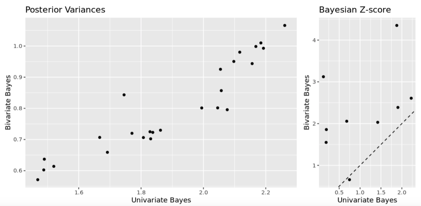
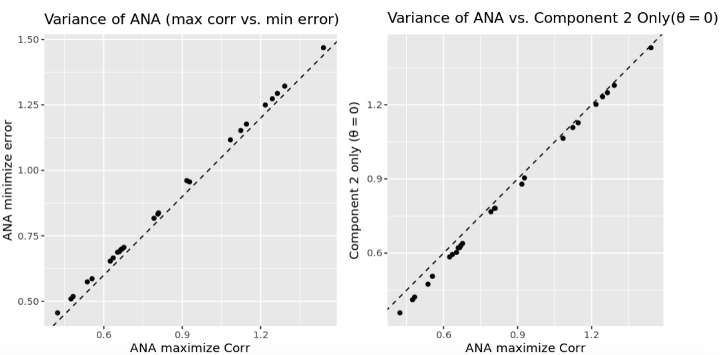
Table 1 demonstrates that using ANA with (), or maximizing correlation, or minimizing error all lead to more statistically significant results, compared to the original before decomposition. Figure 1 shows that the posterior variance is greatly reduced with the bivariate model. Furthermore, the Bayesian Z-score (posterior mean divided by posterior standard deviation) has a greater absolute value under the bivariate model. Figure 2 compares variances of ANA with (), ANA maximizing correlation, and ANA minimizing error. All three produces similar variances.
References
- (1)
- Asmussen and Glynn (2008) Soren Asmussen and Peter Glynn. 2008. Stochastic Simulation. Springer-Verlag.
- Cosgrove et al. (2022) Laura Cosgrove, Jen Townsend, and Jonathan Litz. 2022. Deep Dive Into Variance Reduction. https://www.microsoft.com/en-us/research/group/experimentation-platform-exp/articles/deep-dive-into-variance-reduction/.
- Deng et al. (2023a) Alex Deng, Michelle Du, Anna Matlin, and Qing Zhang. 2023a. Variance Reduction Using In-Experiment Data: Efficient and Targeted Online Measurement for Sparse and Delayed Outcomes. In Proceedings of the 29th ACM SIGKDD Conference on Knowledge Discovery and Data Mining. 3937–3946.
- Deng et al. (2013) Alex Deng, Ya Xu, Ron Kohavi, and Toby Walker. 2013. Improving the sensitivity of online controlled experiments by utilizing pre-experiment data. In Proceedings of the 6th ACM WSDM Conference. 123–132.
- Deng et al. (2023b) Alex Deng, Lo-Hua Yuan, Naoya Kanai, and Alexandre Salama-Manteau. 2023b. Zero to hero: Exploiting null effects to achieve variance reduction in experiments with one-sided triggering. In Proceedings of the Sixteenth ACM International Conference on Web Search and Data Mining. 823–831.
- Guo et al. (2021) Yongyi Guo, Dominic Coey, Mikael Konutgan, Wenting Li, Chris Schoener, and Matt Goldman. 2021. Machine Learning for Variance Reduction in Online Experiments. arXiv preprint arXiv:2106.07263 (2021).
- Jin and Ba (2023) Ying Jin and Shan Ba. 2023. Toward Optimal Variance Reduction in Online Controlled Experiments. Technometrics 65, 2 (2023), 231–242.
- Lin (2013) Winston Lin. 2013. Agnostic notes on regression adjustments to experimental data: Reexamining Freedman’s critique. The Annals of Applied Statistics 7, 1 (2013), 295–318.
- Owen (2013) Art B Owen. 2013. Monte Carlo theory, methods and examples. (2013).
- Poyarkov et al. (2016) Alexey Poyarkov, Alexey Drutsa, Andrey Khalyavin, Gleb Gusev, and Pavel Serdyukov. 2016. Boosted decision tree regression adjustment for variance reduction in online controlled experiments. In Proceedings of the 22nd ACM SIGKDD International Conference on Knowledge Discovery and Data Mining. 235–244.
- Tripuraneni et al. (2023) Nilesh Tripuraneni, Lee Richardson, Alexander D’Amour, Jacopo Soriano, and Steve Yadlowsky. 2023. Choosing a Proxy Metric from Past Experiments. arXiv preprint arXiv:2309.07893 (2023).
- Tsiatis et al. (2008) Anastasios A. Tsiatis, Marie Davidian, Min Zhang, and Xiaomin Lu. 2008. Covariate adjustment for two-sample treatment comparisons in randomized clinical trials: A principled yet flexible approach. Statistics in Medicine 27 (2008).
- Xie and Aurisset (2016) Huizhi Xie and Juliette Aurisset. 2016. Improving the sensitivity of online controlled experiments: Case studies at netflix. In Proceedings of the 22nd ACM SIGKDD International Conference on Knowledge Discovery and Data Mining. ACM, 645–654.