Full Counting Statistics of Charge in Quenched Quantum Gases

Abstract

Unless constrained by symmetry, measurement of an observable in a quantum system returns a distribution of values which are encoded in the full counting statistics. While the mean value of this distribution is important for determining certain properties of a system, the full distribution can also exhibit universal behavior. In this paper we study the full counting statistics of particle number in one dimensional interacting Bose and Fermi gases which have been quenched far from equilibrium. In particular we consider the time evolution of the Lieb-Liniger and Gaudin-Yang models quenched from a Bose-Einstein condensate initial state and calculate the full counting statistics of the particle number within a subsystem. We show that the scaled cumulants of the charge in the initial state and at long times are simply related and in particular the latter are independent of the model parameters. Using the quasi-particle picture we obtain the full time evolution of the cumulants and find that although their endpoints are fixed, the finite time dynamics depends strongly on the model parameters. We go on to construct the scaled cumulant generating functions and from this determine the limiting charge probability distributions at long time which are shown to exhibit distinct non-trivial and non-Gaussian fluctuations and large deviations.

I Introduction

Symmetry and universality are two of the most powerful concepts in theoretical physics. The former can dramatically reduce the complexity of systems, places stringent constraints on allowed physical processes and gives rise to conservation laws via Noether’s theorem. The latter instead explains why vastly different systems can display near identical features and how simple physical principles can underpin many seemingly complex phenomena. These concepts have been extensively studied in the context of closed quantum systems which are close to equilibrium leading to the discovery of many ubiquitous properties and the development of numerous powerful and widely applicable techniques of analysis. In recent years however questions of universality and its emergence in far from equilibrium systems have come to the fore and in this context one-dimensional integrable models have been widely studied [1, 2, 3, 4, 5, 6, 7, 8]. These models possess special symmetry properties endowing them with an infinite number of mutually commuting conserved charges thereby placing strong constraints on their dynamics [9]. At the same time these properties facilitate exact analytic solutions of the models through Bethe ansatz techniques allowing in dept analysis of their thermodynamic properties [10].

Despite this analytic control however, uncovering the non-equilibrium properties of integrable models remains challenging and is still a highly active area of research. Nevertheless many universal features have been established, in particular concerning the dynamics within a subsystem where it has been shown that the system relaxes locally to a stationary state described by a generalized Gibbs ensemble (GGE) [1, 2, 3, 4, 5, 6, 7]. Building upon this a number of exact techniques have been developed including the quench action method [11, 12] which allows one to determine this GGE explicitly and generalized hydrodynamics (GHD) which describes the long time and large scale dynamics of an inhomogeneous state. [13, 14, 15].

A significant driver of interest in the non-equilibrium dynamics of integrable models has been the advent of numerous experimental platforms which allow for the simulation of isolated many-body quantum systems with a high degree of accuracy and control [16, 17, 18]. Chief amongst these are ultra cold atomic gas setups which have the ability to faithfully simulate integrable systems. The Lieb-Liniger model [19] of interacting bosons, the Gaudin-Yang model [20, 21] of interacting fermions and the sine-Gordon field theory [22] are all well known integrable models which can be simulated within cold atom experiments [23, 24, 25, 17, 18, 26, 27, 28, 29, 30, 31, 32, 33, 34]. The relaxation of such models to GGEs [35] as well as the vailidty of GHD [36, 37, 38] has been observed and tested extensively in such experiments ensuring that despite their apparent fine tuned nature integrable models are the appropriate description of these systems.

In this work we shall study the interplay between non-equilibrium dynamics of integrable models and the fluctuations of their charge within a subsystem in the context of cold atom gas experiments. We do this by calculating the full counting statistics (FCS) of the particle number in the Lieb-Liniger (LL) and Gaudin-Yang (GY) models. The systems shall be taken out of equilibrium by quenching them from an initial Bose-Einstein condensate (BEC) state which is not only experimentally relevant and conceptually simple but also allows us to characterize the dynamics exactly. We shall show that there exists a simple relationship between the cumulants of charge in the initial state and the GGE to which these systems relax at long times. This relationship is in fact universal, relying only on the presence of integrability and not on details of the model. However, while the cumulants in the final state are fixed by the initial state their decomposition in terms of quasi-particle excitations differs from model to model meaning that the finite time dynamics will differ.

Moreover, since the leading order (linear in subsystem size) behavior of the cumulants of charge fluctuations in the GGEs are the same in all cases they define the same limiting coarse-grained or continuous probability distributions (PDs) which can be explicitly determined. Nevertheless, the microscopic PDs (retaining information about sub-leading corrections) can be different. This fact arises from the transmutation of particle statistics in the different parameter regimes of each model and manifests in a simple and intuitive way. For example, in the strongly attractive Fermi gas the fermions are bound into tight pairs forming hard core bosons with double the charge, a fact which is reflected in vanishing probabilities for observing an odd number of particles in a subsystem.

The rest of the paper is arranged as follows: In Sec. II we review our object of study, the full counting statistics and some basic properties of cumulant generating functions and their associated probability distributions. We also briefly recall some properties of integrable models and prove a general relationship between the FCS calculated in a GGE and in the diagonal ensemble. In Sec. III we introduce the models we shall study as well as the particular initial states of interest. In Sec. IV we determine the cumulants of charge in Lieb-Liniger model for both repulsive and attractive regimes. In Sec. V we carry out an analogous calculation in the repulsive and attractive regimes of the Gaudin-Yang model. In the penultimate section we study the analytic properties of the scaled cumulant generating functions for both our models. We use this knowledge to determine the limiting charge probability distributions in both the initial and final states. In the last section we summarize our work and discuss open questions and potential future directions.

II Non-equilibrium Full Counting Statistics in integrable models

We wish to characterize the fluctuations of the particle number in the LL and GY models which have been quenched from BEC states. While these charges are conserved quantities for the full system, when we restrict to a subsystem they exhibit nontrivial fluctuations and dynamics [39, 40, 41, 42, 43, 44, 45, 46, 47, 48, 49, 50, 51, 52, 53, 54, 55, 56, 57]. To study this we calculate the full counting statistics of the charge within a region $A$ of length $\ell$. We take $\ell$ to be large but much smaller than the full system, $1\ll\ell\ll L$ where $L$ is the full system size and in the end take the thermodynamic limit $\ell,L\to\infty$. For a charge operator $\hat{N}$ whose restriction to the subsystem is denoted $\hat{N}_{A}$ the FCS are defined as

$$Z_{\beta}(A,t)=\tr[\rho_{A}(t)e^{\beta\hat{N}_{A}}]$$ (1)

where $\rho_{A}(t)=\tr_{\bar{A}}[\rho(t)]$ is the reduced density matrix of $A$ at time $t$ and $\rho(t)=\outerproduct{\Psi_{0}(t)}{\Psi_{0}(t)}$ is the density matrix of the full system which has been quenched from the intial state $\ket{\Psi_{0}}\to\ket{\Psi_{0}(t)}=e^{-iHt}\ket{\Psi_{0}}$. While the FCS of charge and related quantities like the work distribution have been studied previously in certain interacting integrable models [58, 59, 48, 60, 61, 62, 63], recent developments have allowed to study these quantities in far from equilibrium systems as well as their associated current statistics [64, 65, 50, 66, 67, 68, 69, 70, 71, 72].

From the FCS we can determine many properties of the dynamics of the particle number fluctuations within the subsystem and its interplay with the relaxation of the system to its long time steady state. Specifically, we can calculate the connected correlation functions of the charge via the cumulants of the FCS,

$$\left<N_{A}^{m}(t)\right>^{c}=\partial_{\beta}^{m}\log Z_{\beta}(A,t)|_{\beta=0}$$ (2)

for $m\in\mathbb{N}$ and where $\left<\cdot\right>^{c}$ means the connected part of the correlation function e.g. $\left<N_{A}^{2}(t)\right>^{c}=\left<N_{A}^{2}(t)\right>-\left<N_{A}(t)\right>^{2}$. Moreover, by continuing $\beta\to i\beta$ we can obtain the charge probability distribution $P(n,t)$,

$$P(n,t)=\int_{-\pi}^{\pi}\frac{{\rm d}\beta}{2\pi}e^{-i\beta n}Z_{i\beta}(A,t)$$ (3)

which gives the probability that a measurement of $\hat{N}_{A}$ at time $t$ returns the value $n$. The latter is a natural quantity to study from the experimental point of view and particularly so in the case of cold atom experiments. While the expectation value of an observable such as an order parameter is a central quantity to understand the nature of a system, the full distribution of measurement outcomes is also enlightening and can unveil universal behavior. In cold atom experiments large numbers of measurements are required to be performed and so the full probability distribution is naturally obtained [73].

By our analytical methods which we shall introduce shortly, the computation of the cumulants or the cumulant generating function $\log Z_{\beta}(A,t)$ is only feasible if the length of the subsystem $\ell$ is also infinitely large. In particular, the moment generating function for an extensive quantity in a large subsystem can be generally written as

$$\lim_{\ell\rightarrow\infty}Z_{\beta}(A,t)=e^{\ell C^{s}(\beta,t)+o(\ell)}$$ (4)

where $C^{s}(\beta,t)$ is the scaled cumulant generating function (SCGF) defined as

$$\lim_{\ell\rightarrow\infty}\ell^{-1}\log Z_{\beta}(A,t)=C^{s}(\beta,t)$$ (5)

and whose derivatives wrt. $\beta$ are the scaled cumulants

$$\partial^{m}_{\lambda}C^{s}(\beta,t)|_{\lambda=0}=\kappa^{s}_{m}(t)$$ (6)

denoted by $\kappa^{s}_{m}$. Therefore it is the scaled cumulants and their generating function, i.e., quantities with extensive scaling w.r.t. the subsystem size, which can be computed. From the SCGF, we can obtain the large $\ell$ limiting probability distribution (PD) for the charge fluctuations via the rate function $I(z)$ through

$$P(\ell z,\ell t)\asymp e^{-\ell I(z,t)}$$ (7)

where $\asymp$ is understood as

$$a(\ell,x)\asymp b(\ell,x)\,\,\text{if}\,\,\lim_{\ell\rightarrow\infty}\frac{\log\,a}{\log\,b}=1\,,$$ (8)

and we assumed the same scaling for the time variable $t$. Importantly the rate function $I(z)$ can be obtained as the Legendre-Fenchel transform of the SCGF according to the Gärtner-Ellis theorem. The rate function also governs the large deviations of the limiting coarse-grained probability distribution, which is a continuous distribution even if the microscopic PD is discrete. Whereas in a strict sense our methods allow for the computation of $I(z)$ via the SCGFs, we shall also use Eq. (3) and approximate $Z_{i\beta}(A,t=0,\infty$) at the initial and the steady-states by $\exp\left(\ell C^{s}(i\beta,t=0,\infty)\right)$. Doing so retains the discrete nature of charge fluctuations and allows for the onset of some interesting microscopic effects, which vanish in the $\ell\rightarrow\infty$ limit but are expected to be observed in large but finite subsystems.

In the subsequent sections we shall explicitly calculate the scaled cumulants $\kappa_{m}^{s}(t)$ as well as SCGF $C^{s}(\beta,t=0,\infty)$ in the LL and GY models however before this we shall derive some generic properties which will allow us to relate the scaled cumulants in the initial state, denoted by $\kappa^{s}_{m}(0)$, and in the GGE, denoted by $\kappa^{s}_{m}(\infty)$. To do this we keep things general and recall briefly some basic properties of integable models: Integrable models posses an extensive number of conserved quantities charges whose associated operators $\hat{Q}^{(k)},~{}k=1,2,\dots$ commute with the Hamiltonian. These imbue the model with a stable set of quasi-particle excitations which are indexed by a discrete species index $n=1,\dots,N_{s}$ and parameterized by a continuous rapidity $\lambda^{(n)}_{j}$, $j=1,\dots,M_{n}$. An eigenstate of the model is specified by the rapidities of the quasi-particles which are present, we denote it by

$$\ket{\bm{\lambda}}=\ket*{\lambda^{(1)}_{1},\ldots,\lambda^{(1)}_{M_{1}};\ldots;\lambda^{(N_{s})}_{1},\ldots,\lambda^{(N_{s})}_{M_{N_{s}}}}.$$ (9)

These states are also simultaneous eigenstates of all the conserved charges of the model. Namely

$$\hat{Q}^{(k)}\ket{\bm{\lambda}}=\sum_{n=1}^{N_{s}}\sum_{j=1}^{M_{m}}q_{n}^{(k)}(\lambda^{(m)}_{j})\ket{\bm{\lambda}}.$$ (10)

The first three conserved charges are chosen to coincide with the particle number $\hat{N}=\hat{Q}^{(0)}$, momentum $\hat{P}=\hat{Q}^{(1)}$ and Hamiltonian $\hat{H}=\hat{Q}^{(2)}$. For simplicity we shall denote the charge, momentum and energy of a quasi-particle of species $n$ and rapidity $\lambda$ by $q_{n}=q^{(0)}_{n}(\lambda),p_{n}(\lambda)=q^{(1)}_{n}(\lambda)$ and $\epsilon_{n}(\lambda)=q^{(2)}_{n}(\lambda)$. In the thermodynamic limit and at finite density the quasi-particle content of a stationary state of the model can instead be encoded in the distributions $\rho_{n}(\lambda),\rho_{n}^{h}(\lambda),\rho_{n}^{t}(\lambda)$ and $\vartheta_{n}(\lambda)$ which are respectively the distribution of occupied quasiparticles of species $n$, the distribution unoccupied quasiparticles, the total density of states $\rho_{n}^{t}(\lambda)=\rho_{n}(\lambda)+\rho_{n}^{h}(\lambda)$ and the occupation function $\vartheta_{n}(\lambda)=\rho_{n}(\lambda)/\rho^{t}_{n}(\lambda)$. All of these functions are related to each other by the Bethe-Takahashi equations which take the form

$$\rho^{t}_{n}(\lambda)=\frac{p_{n}^{\prime}(\lambda)}{2\pi}-\sum_{l}\mathcal{T}_{nl}*\rho_{l}(\lambda)$$ (11)

where $(\cdot)^{\prime}$ denotes differentiation w.r.t. $\lambda$ and $*$ is the convolution $f*g(y)=\int{\rm d}yf(x-y)g(y)$. Here $\mathcal{T}_{nl}(\lambda,\mu)$ is the scattering kernel which characterizes the scattering between quasi-particles of type $n$ and $l$ with rapidities $\lambda$ and $\mu$. In the cases of interest this is symmetric in the species index $\mathcal{T}_{nl}(x)=\mathcal{T}_{ln}(x)$.

When the state contains many excitations the bare quasi-particle properties become dressed due to the interactions. These dressed quantities are denoted by $(\cdot)^{\rm dr}$ and satisfy the integral equations

$$f_{n}^{\rm dr}(\lambda)=f_{n}(\lambda)-\sum_{l}\mathcal{T}_{nl}*[\vartheta_{l}(\lambda)f_{l}^{\rm dr}(\lambda)].$$ (12)

Explicitly, the dressed charge is obtained from the solution of

$$q^{\rm dr}_{n}(\lambda)=q_{n}-\sum_{l}\mathcal{T}_{nl}*[\vartheta_{l}(\lambda)q_{l}^{\rm dr}(\lambda)].$$ (13)

The quasi-particle velocity on the other hand is given by the ratio of dressed quantities, $v_{n}(\lambda)={\epsilon^{\prime}}^{\rm dr}(\lambda)/{p^{\prime}}^{\rm dr}(\lambda)$. This can be recast into the equation

$$\rho^{t}_{n}(\lambda)v_{n}(\lambda)=\frac{\epsilon_{n}^{\prime}(\lambda)}{2\pi}-\sum_{l}\mathcal{T}_{nl}*[\rho_{l}(\lambda)v_{l}(\lambda)]$$ (14)

where we have used $\rho^{t}(\lambda)={p^{\prime}}^{\rm dr}(\lambda)$. These sets of integral equations typically need to be solved numerically but in certain cases can be solved analytically as is the case for the LL model discussed below [74, 75, 76].

Having reviewed these basic properties and set up our notation we can now move on to determine the relationship between the FCS at $t=0$ and in the GGE. We begin with the latter and define

$$\lim_{t\to\infty}\tr[e^{\beta\hat{N}_{A}}\rho_{A}(t)]=\tr[e^{\beta\hat{N}_{A}}\rho_{\rm GGE}]\equiv\exp\left(\ell C^{s}_{\text{GGE}}(\beta)\right)$$ (15)

where we have neglected the $o(\ell)$ contributions and have introduced the generalized Gibbs ensemble

$$\rho_{\rm GGE}=\frac{1}{\tr[e^{\sum_{k}\beta^{(k)}\hat{Q}^{(k)}}]}e^{\sum_{k}\beta^{(k)}\hat{Q}^{(k)}}.$$ (16)

Herein it is necessary to include both local and semi-local conserved charges in the GGE in order to obtain the correct description of the long time state [77, 78, 79, 80, 81]. The Lagrange multipliers above, $\beta^{(k)}$, are determined by matching the expectation values of $\hat{Q}^{(k)}$ in $\rho_{\rm GGE}$ to those in the initial state. To compute $C^{s}_{\text{GGE}}(\beta)$ with $\beta\in\mathbb{R}$ we utilise the result of Ref. [64] (see also [82, 55]) claiming that

$$C^{s}_{\text{GGE}}(\beta)=f_{\text{GGE}}(\underline{\beta}^{(k)}+\beta)-f_{\text{GGE}}(\underline{\beta}^{(k)})$$ (17)

where $f_{\text{GGE}}$ denotes the free energy density of a GGE characterized by the chemical potentials $\underline{\beta}^{(k)}$ and $\beta$ shifts one of the chemical potentials that corresponds to the conserved quantity under investigation. We can rewrite the above equations in the typical manner of the thermodynamic Bethe ansatz by exchanging the trace for a path integral over the distributions $\rho_{n}(\lambda),\rho^{h}_{n}(\lambda)$ [10],

$$e^{\ell C^{s}_{\text{GGE}}(\beta)}=\frac{\int\mathcal{D}[\rho(\lambda)]e^{-\ell\sum_{n}\int{\rm d}\lambda(g_{n}(\lambda)-\beta q_{n})\rho_{n}(\lambda)-S_{YY}}}{\int\mathcal{D}[\rho(\lambda)]e^{-\ell\sum_{n}\int{\rm d}\lambda g_{n}(\lambda)\rho_{n}(\lambda)-S_{YY}}}$$ (18)

where $g_{n}(\lambda)=\sum_{k}\beta^{(k)}q^{(k)}_{n}(\lambda)$ and $S_{YY}$ is the Yang-Yang entropy which is proportional to $\ell$ as well and which counts how many microstates $\ket{\bm{\lambda}}$ correspond to the same macrostate given by the distributions $\rho_{n}(\lambda)$. Evaluating this functional integral via a saddle point approximation we obtain

$$C^{s}_{\text{GGE}}(\beta)=\!\sum_{n=1}^{N_{s}}\int\!\!{\rm d}\lambda\rho^{t}_{n}\!\!\left[\!\log\!\left(\frac{1+\eta^{-1}_{n,\beta}}{{1+\eta^{-1}_{n,0}}}\right)\!+\vartheta_{n}\!\log\frac{\eta_{n,\beta}e^{\beta q_{n}}}{\eta_{n,0}}\!\right]$$ (19)

with $\eta_{n,\beta}$ being given by

$$\log\eta_{n,\beta}=-\beta q_{n}+g_{n}(\lambda)+\sum_{l}\mathcal{T}_{nl}*\log[1+\eta^{-1}_{l,\beta}(\lambda)]\,,$$ (20)

while $\eta_{n,0}$ is evaluated in the same way at $\beta=0$ and can be related to the occupation function of the GGE via $\vartheta_{n}(\lambda)=1/(1+\eta_{n,0}(\lambda))$. In order to evaluate $C^{s}_{\text{GGE}}(\beta)$ explicitly one must know the functional form of $g_{n}(\lambda)$ which can be done by making use of the quench action method. Using this one can show that it is obtained from the extensive part the squared overlap between an eigenstate $\ket{\bm{\lambda}}$ and $\ket{\Psi_{0}}$ in the thermodynamic limit [83]. Namely,

$$\lim_{\rm th}\frac{1}{L}\log|\innerproduct{\bm{\lambda}}{\Psi_{0}}|^{2}=-\frac{1}{2}\sum_{n=1}^{N_{s}}\int{\rm d}\lambda\,g_{n}(\lambda)\rho_{n}(\lambda).$$ (21)

For the states that we consider the left hand side is known explicitly and the function $g_{n}(\lambda)$ is simply extracted from this.

We now turn to the calculation of the FCS in the initial state. In this instance, as discussed further in Appendix A, the initial value can be obtained by considering the diagonal ensemble. After expressing this as a path integral we find

$$e^{\ell C^{s}_{0}(\beta)}=\frac{\int\mathcal{D}[\rho(\lambda)]e^{-\frac{\ell}{2}\sum_{n}\int{\rm d}\lambda(g_{n}(\lambda)-2\beta q_{n})\rho_{n}(\lambda)-\frac{1}{2}S_{YY}}}{\int\mathcal{D}[\rho(\lambda)]e^{-\frac{\ell}{2}\sum_{n}\int{\rm d}\lambda g_{n}(\lambda)\rho_{n}(\lambda)-\frac{1}{2}S_{YY}}}$$ (22)

where the factor of $\frac{1}{2}$ in front of $S_{YY}$ arises from the fact that the overlap with our initial state is non-zero only for parity invariant eigenstates which have half the entropy contribution. Here we have denoted $C^{s}(\beta,0)$ by $C^{s}_{0}(\beta)$, which we express more explicitly as

$$C^{s}_{0}(\beta)=\frac{1}{2}\sum_{n=1}^{N_{s}}\int\!\!{\rm d}\lambda\bar{\rho}^{t}_{n}\!\!\left[\!\log\!\left(\frac{1+\bar{\eta}^{-1}_{n,\beta}}{{1+\bar{\eta}^{-1}_{n,0}}}\right)\!+\bar{\vartheta}_{n}\!\log\frac{\bar{\eta}_{n,\beta}e^{2\beta q_{n}}}{\bar{\eta}_{n,0}}\!\right]$$ (23)

with $\bar{\eta}_{n,\beta}$ being given by

$$\log\bar{\eta}_{n,\beta}=-2\beta q_{n}+g_{n}(\lambda)+\sum_{l}\mathcal{T}_{nl}*\log[1+\bar{\eta}^{-1}_{l,\beta}(\lambda)]\,.$$ (24)

Either comparing Eqs. (18) and (22) or the TBA systems (19) and (23), we then find that

$$C^{s}_{0}(\beta)=\frac{1}{2}C^{s}_{\text{GGE}}(2\beta)$$ (25)

where $C^{s}_{\text{GGE}}$ is given by (19). Therefore comparing with (15) we also find that the cumulants are related as

$$\kappa^{s}_{m}(\infty)=\frac{1}{2^{m-1}}\kappa^{s}_{m}(0).$$ (26)

The above relations are one of the main results of this paper.

A notable consequence of the relations is that since the right hand sides of (25) and (26) are a property solely of the initial state then the left hand side is independent of the model specifics. In the examples below we shall argue and then show explicitly that for BEC initial states $\kappa_{m}^{s}(0)=d$ $\forall m$ where $d$ is the average density i.e., the charge is Poisson distributed and accordingly

$$\kappa_{m}^{s}(\infty)=\frac{d}{2^{m-1}}\,,$$ (27)

which is exactly the same expression as the one obtained from the steady-state GGE using (17) as we shall demonstrate shortly.

Evidently (26) does not tells us how the charge distribution evolves between its initial value and the GGE value which necessarily depends on the model. However we can also characterize this in integrable models using recently obtained results on the charged moments and full counting statistics using the method of space-time duality [55, 56]. In particular the scaled cumulants obey a quasi-particle picture [84, 85] meaning that charge fluctuations are spread throughout the system via the ballistic propagation of pairs of quasi-particles which are shared between $A$ and $\bar{A}$ resulting in

$$\left<N^{m}_{A}(t)\right>^{c}\approx\ell\kappa^{s}_{m}(t)=\ell\kappa^{s}_{m}(0)\quad\quad\quad\quad\quad\quad\quad\quad\quad\quad\quad$$

$$+\ell\sum_{n}\int\mathrm{d}\lambda\,{\rm min}[2t|v_{n}(\lambda)|,\ell]\left(\mathcal{K}^{m}_{n,\infty}(\lambda)-\mathcal{K}^{m}_{n,0}(\lambda)\right)$$ (28)

where we have introduced $\mathcal{K}^{m}_{n,{\rm x}}(\lambda)$ with ${\rm x}=0,\infty$ being the rapidity and species resolved scaled cumulant in the initial state or GGE, i.e.

$$\kappa^{s}_{m}({\rm x})=\sum_{n}\int\mathrm{d}\lambda\,\mathcal{K}^{m}_{n,{\rm{x}}}(\lambda).$$ (29)

Additionally, ${\rm min}[2t|v_{n}(\lambda)|,\ell]$ is the characteristic function which counts the number of quasi-particle pairs shared between $A$ and $\bar{A}$.

The first cumulant returns the expectation value of the charge and is conserved which can be seen using (27) and (28) at $m=1$. The second cumulant gives the charge susceptibility which has a compact expression

$$\mathcal{K}_{n,\infty}^{2}(\lambda)=[q_{n}^{\rm dr}(\lambda)]^{2}\rho_{n}(\lambda)(1-\vartheta_{n}(\lambda)).$$ (30)

Higher cumulants become more complicated and involve dressing of lower cumulants. For example, the third cumulant is given by

$$\frac{\mathcal{K}_{n,\infty}^{3}(\lambda)}{\mathcal{K}_{n,\infty}^{2}(\lambda)}=q_{n}^{\rm dr}(\lambda)(1-2\vartheta_{n}(\lambda))-\frac{3[\sum_{l}\mathcal{T}_{nl}*\mathcal{K}_{l,\infty}^{2}]^{\rm dr}(\lambda)}{q_{n}^{\rm dr}(\lambda)}$$

where we see that it depends also on the dressed second cumulant. We omit higher expressions for cumulants which can nevertheless be systematically computed.

Before moving on, we make two brief remarks on the preceding discussion. First, the result (26) relies upon the validity of the diagonal ensemble for calculating the initial state value which is discussed further in Appendix A. To check the validity of (26) we shall compute the scaled cumulants in the initial states by independent means and show that the results of the diagonal ensemble, involving interaction-dependent functions, yield the same result. This is not always the case however and the diagonal ensemble cannot be applied to initial states such that the subsystem is an eigenstate of the charge and hence has no fluctuations. This is the case for the magnetization of the GY model quenched from the BEC state. However for the models and initial states which we consider the diagonal ensemble correctly reproduces the initial FCS of the particle number. Second, although some analytic results exist for the distributions functions which determine (19) and (22), their explicit evaluation is feasible only in certain special limits of our models. In spite of this, at generic interactions, it is straightforward to numerically compute the (first few) scaled cumulants and check the validity of (26). The numerical computation of the SCGF is also possible but instead of comparing the numerically obtained SCGFs against (25) on a strictly finite interval, we shall rather construct the SCGFs at arbitrary interactions as a Taylor series defined by the cumulants, which is justified by the exponentially decaying behavior of the scaled cumulants.

III Models and Setup

III.1 Lieb-Liniger model

The standard model for describing one-dimensional interacting bosons in the context of cold atom experiments is the Lieb-Liniger model. The Hamiltonian is given by

$$H_{LL}\!=\!\!\int_{0}^{L}\!\!\!\!{\rm d}x\,b^{\dagger}(x)\!\!\left[-\frac{\partial_{x}^{2}}{2m}\right]\!b(x)+cb^{\dagger}(x)b(x)b^{\dagger}(x)b(x).$$ (31)

Here $b^{\dagger}(x),b(x)$ are canonical bosonic operators satisfying $[b(x),b^{\dagger}(y)]=\delta(x-y)$ they describe bosons of mass $m$ which interact via a density-density interaction of strength $c$ on a system of length $L$. We shall consider both the repulsive $c>0$ and attractive $c<0$ cases. From here on we take $m=1/2$ for simplicity and assume periodic boundary conditions. The model has a single $U(1)$ charge, the particle number $\hat{N}=\int{\rm d}x\,b^{\dagger}(x)b(x)$.

In the repulsive case there is only one species of quasi-particle with bare charge, momentum and energy given by

$$q=1,~{}p(\lambda)=\lambda,~{}\epsilon(\lambda)=\lambda^{2}.$$ (32)

As outlined above, the properties of a stationary state of $H$ are encoded in the distributions $\rho(\lambda),\rho^{h}(\lambda),\rho^{t}(\lambda)$ and $\vartheta(\lambda)$ which are connected via the Bethe equations

$$\rho^{t}(\lambda)=\frac{1}{2\pi}+\int_{-\infty}^{\infty}{\rm d}\mu\,a_{2}(\lambda-\mu)\rho(\mu)$$ (33)

where the scattering kernel is given by $a_{n}(x)=\frac{1}{2\pi}\frac{n|c|}{(nc/2)^{2}+x^{2}}$.

In the attractive case the spectrum of the model is entirely different and there are an infinite number of quasi-particle species corresponding to bound states of $n$ bosons. These quasi-particles have the following bare charge, momentum and energy

$$q_{n}=n,~{}p_{n}(\lambda)=n\lambda,~{}\epsilon_{n}(\lambda)=n\lambda^{2}+\frac{|c|}{12}n(n^{2}-1).$$ (34)

We denote the distributions of the $n$-boson bound states by $\rho_{n}(\lambda),\rho_{n}^{h}(\lambda),\rho_{n}^{t}(\lambda)$ and $\vartheta_{n}(\lambda)$. The Bethe equations in this case then take the form

$$\rho^{t}_{n}(\lambda) = \frac{n}{2\pi}-\sum_{m=1}^{\infty}T_{nm}*\rho_{m}(\lambda)$$ (35)

where for $n>m$ the two particle scattering kernel is

$$T_{mn}(\lambda) = a_{n-m}(\lambda)+a_{n+m}(\lambda)+2\sum_{j=1}^{m-1}a_{n-m+2j}(\lambda),$$

$$T_{nn}(\lambda) = 2\sum_{j=1}^{n}a_{2j}(\lambda),\quad T_{mn}(\lambda)=T_{nm}(\lambda).$$ (36)

We shall study the dynamics of the system quenched from the BEC state of $N$ particles given by

$$\ket{\Psi_{0,N}} = \frac{{b^{\dagger}_{0}}^{N}}{\sqrt{N!}}\ket{0},$$ (37)

$$b_{0}^{\dagger} = \frac{1}{\sqrt{L}}\int_{0}^{L}{\rm d}x\,b^{\dagger}(x)$$ (38)

which is the ground state of the model at $c=0$ and is also an eigenstate of $\hat{N}$. When considering just the subsystem however $\rho_{A}(0)$ contains states in all particle number sectors less than $N$ and the charge probability distribution can be determined by means of a simple argument. Since the wavefunction is constant the probability of measuring a charge in $A$ for the system with $N=1$ is given by $\ell/L$. For higher particle number since the state has no spatial correlations the detection of a boson is an independent event with a constant rate $\ell N/L$ and therefore has a binomial distribution. In the thermodynamic limit we take $N,L\to\infty$ with $d=N/L$ the density held fixed and thus we end up with a Poisson distribution with rate $\ell d$ and $\left<N^{m}_{A}\right>^{c}_{0}=\ell d$ or $\kappa^{s}_{m}(0)=d,~{}\forall m$.

From this observation it is possible to construct the reduced density matrix $\rho_{A}(0)$. Introducing the boson on the restricted space $\bar{b}^{\dagger}_{0}=\frac{1}{\sqrt{\ell}}\int_{x\in A}{\rm d}x\,b^{\dagger}(x)$ we have that

$$\rho_{A}(0)=e^{-\ell d}\sum_{n=0}^{\infty}\frac{(\ell d)^{2n}}{n!^{2}}{{\bar{b}}^{\dagger}_{0}}{}^{n}\outerproduct{0_{A}}{0_{A}\!}{{\bar{b}_{0}}}{}^{n}$$ (39)

where $\ket{0_{A}}$ is the vacuum inside $A$. This has the required Poisson distribution of charge and also has the same correlation within the subsystem as $\outerproduct{\Psi_{0}}{\Psi_{0}}$.

The entanglement entropy between $A$ and $\bar{A}$ can also be determined from this expression and originates solely from the charge fluctuations in the subsystem. The von Neumann entanglement entropy is given by Shannon entropy of the charge probability distribution and so scales as $S_{A}\simeq\frac{1}{2}+\frac{1}{2}\log 2\pi\ell d$.

III.2 Gaudin-Yang model

For the case of interacting spinful fermions in one dimension we shall study the Gaudin-Yang model which is also widely used to describe cold atom gas experiments. The Hamiltonian is

$$H_{GY}\!=\!\!\int_{0}^{L}\!\!\!{\rm d}x\,\psi_{\sigma}^{\dagger}(x)\!\!\left[\!-\frac{\partial_{x}^{2}}{2m}\right]\!\!\psi_{\sigma}(x)+c\psi_{\uparrow}^{\dagger}(x)\psi_{\uparrow}(x)\psi_{\downarrow}^{\dagger}(x)\psi_{\downarrow}(x)$$ (40)

where $\psi_{\sigma}^{\dagger}(x),\psi_{\sigma}(x)$ are two species of fermionic operators with $\sigma=\uparrow,\downarrow$ which obey $\{\psi^{\dagger}(x)_{\sigma},\psi_{\sigma^{\prime}}(y)\}=\delta_{\sigma\sigma^{\prime}}\delta(x-y)$. These describe spin $1/2$ fermions of mass $m$ interacting via a local inter-species density-density interaction of strength $c$. As before we shall take $m=1/2$ and assume periodic boundary conditions but we shall consider both repulsive $c>0$ and attractive $c<0$ interactions. In this case there are two $U(1)$ conservation laws corresponding to particle number $\hat{N}=\int{\rm}dx\,\psi_{\uparrow}^{\dagger}(x)\psi_{\uparrow}(x)+\psi_{\downarrow}^{\dagger}(x)\psi_{\downarrow}(x)$ and magnetization $\hat{M}=\int{\rm}dx\,\psi_{\uparrow}^{\dagger}(x)\psi_{\uparrow}(x)-\psi_{\downarrow}^{\dagger}(x)\psi_{\downarrow}(x)$, however we shall only concentrate on the former.

The quasi-particle content of the model depends on whether one is in the repulsive regime or attractive. In the repulsive regime there are an infinite number of species and we denote their distributions by $\rho(\lambda),\rho^{h}(\lambda),\rho^{t}(\lambda),\vartheta(\lambda)$ and $\sigma_{n}(\lambda),\sigma^{h}_{n}(\lambda),\sigma^{t}_{n}(\lambda),\vartheta_{n}(\lambda)$ where $n\in\mathbb{N}$. The former type of quasi-particles are associated to spin up fermions, they have unit charge and magnetization and momentum and energy $p(\lambda)=\lambda,\epsilon_{n}(\lambda)=\lambda^{2}$. The latter quasi-particle types, also called strings are associated to the spin degrees of freedom, they carry zero charge, magnetization $-2n$ and have zero energy and momentum. The integral equations for these distributions are

$$\rho^{t}(\lambda) = \frac{1}{2\pi}+\sum_{n=1}^{\infty}a_{n}*\sigma_{n}(\lambda)$$ (41)

$$\sigma^{t}_{n}(\lambda) = a_{n}*\rho(\lambda)-\sum_{m=1}^{\infty}T_{nm}*\sigma_{m}(\lambda)$$ (42)

where for $T_{nm}(\lambda)$ was introduced above In terms of these distributions the $U(1)$ charges of a state are given by $N=\int{\rm d}\lambda\rho(\lambda)$ and $M=N-2\sum_{n=1}^{\infty}n\int{\rm d}\lambda\,\sigma_{n}(\lambda)$.

In the attractive regime there is an additional type of quasi-particle which is a bound state of two fermions forming a spin singlet. We denote its distributions by $\tilde{\rho}(\lambda)\tilde{\rho}^{h}(\lambda),\tilde{\rho}^{t}(\lambda),\tilde{\vartheta}(\lambda)$. They carry charge $2$ and magnetization $0$ while their momentum and energy are $\tilde{p}(\lambda)=2\lambda,~{}\tilde{\epsilon}(\lambda)=2\lambda^{2}$. The corresponding integral equations are

$$\rho^{t}(k) = \frac{1}{2\pi}-a_{1}*\tilde{\rho}(\lambda)-\sum_{n=1}^{\infty}\,a_{n}*\sigma_{n}(\lambda)$$ (43)

$$\tilde{\rho}^{t}(\lambda) = \frac{1}{\pi}-a_{2}*\tilde{\rho}(\lambda)-a_{1}*\rho(\lambda)$$ (44)

$$\sigma^{t}_{n}(\lambda) = a_{n}*\rho(\lambda)-\sum_{m=1}^{\infty}T_{nm}*\sigma_{m}(\lambda).$$ (45)

For the fermionic model we shall again study the dynamics emerging from a BEC state wherein the bosons are formed from pairs of fermions in a singlet at the same point in space,

$$\ket{\Phi_{0,N}} = \frac{{c^{\dagger}_{0}}^{N}}{\sqrt{N!}}\ket{0},$$ (46)

$$c_{0}^{\dagger} = \frac{1}{\sqrt{\mathcal{N}_{L}}}\int_{0}^{L}{\rm d}x\,\psi_{\uparrow}^{\dagger}(x)\psi_{\downarrow}^{\dagger}(x)$$ (47)

where $\mathcal{N}_{L}$ is a normalization factor. In contrast to the previous case this is not an eigenstate of the model at any $c$ but is an eigenstate of particle number $\matrixelement{\Phi_{0,N}}{\hat{N}}{\Phi_{0,N}}=2N$ and magnetization $\matrixelement{\Phi_{0,N}}{\hat{M}}{\Phi_{0,N}}=0$. Once again upon tracing out $\bar{A}$, particle number is no longer conserved however the magnetization is still $0$. In this instance the wavefunction is not flat due to the Pauli exclusion of the fermions however for large enough subsystem size and at finite density we can apply the same arguments as before and determine that the charge distribution is also Poisson. In particular, it is easy to check analytically the first few cumulants, which, in the thermodynamic limit, in fact yield $\kappa_{m}(0)=2d$ if $d$ denotes the density of singlet pairs. Furthermore the initial reduced density matrix has the form

$$\rho_{A}(0) = e^{-\ell d}\sum_{n=0}^{\infty}\frac{{(\ell d)}^{2n}}{n!^{2}}{{\bar{c}}^{\dagger}_{0}}{}^{n}\outerproduct{0_{A}}{0_{A}}{{\bar{c}}_{0}}{}^{n},$$ (48)

$$\bar{c}^{\dagger}_{0} = \frac{1}{\sqrt{\mathcal{N}_{\ell}}}\int_{x\in A}\!\!\!\!{\rm d}x\,\psi_{\uparrow}^{\dagger}(x)\psi_{\downarrow}^{\dagger}(x)\,\,.$$ (49)

In other words, we have again obtained constant cumulants, which can be attributed to a Poisson distribution. It is, nevertheless, important to recall the fact that for any subsystem, the total magnetization is zero, which means that the distribution is only Poissonian for the effective ‘quasi-bosons’. Therefore the fermionic distribution is microscopically different, namely it has vanishing probabilities for odd fermion numbers. In the thermodynamic limit, this distribution can have the same cumulants and scales to the same limiting continuous PD, determined by the rate function of the Poisson distribution with density $2d$. We shall revisit this feature in Sec. VI. The von Neumann entanglement entropy can be obtained here also and similarly coincides with the Shannon entropy of the Poisson distribution.

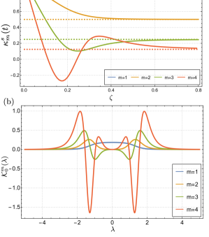
Figure 1: (a): The scaled cumulants, $\kappa_{m}^{s}(t),~{}m=1,\dots 4$ as a function of rescaled time $\zeta=t/\ell$ for $d=1$ and $c=1$. The dashed lines are the asymptotic GGE values. (b): The rapidity resolved scaled cumulants, $\mathcal{K}^{m}_{0}(\lambda)$ as a function of $\lambda$ for $m=1,\dots,4$ for $c=1,d=1$.

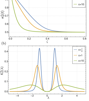
Figure 2: (a): The scaled second cumulant, $\kappa^{s}_{2}(t)$ as a function of rescaled time $\zeta=t/\ell$ for $d=1$ and $c=\frac{1}{2},1,10$. (b): the rapidity resolved cumulant, $\mathcal{K}^{2}_{0}(\lambda)$ as a function of $\lambda$ for $c=\frac{1}{2},1,10$.

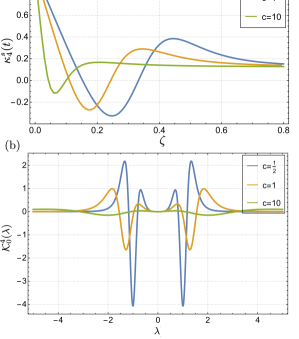
Figure 3: (a): The fourth scaled cumulant, $\kappa^{s}_{4}(t)$ as a function of rescaled time $\zeta=t/\ell$ for $d=1$ and $c=\frac{1}{2},1,10$. (b): The rapidity resolved cumulant, $\mathcal{K}^{4}_{0}(\lambda)$ as a function of $\lambda$ for $c=\frac{1}{2},1,10$.

IV FCS in the Lieb-Liniger model

We now turn to the explicit calculation of the SCGF in the Lieb-Liniger model treating the repulsive and attractive regimes separately. The quench dynamics emerging from the state (37) has been studied previously in both the repulsive [74] and attractive cases [75, 76] with many properties already determined analytically and with thorough discussion on the steady-state GGE in the repulsive case [86]. Below we shall make use of these exact results to obtain the FCS.

IV.1 Repulsive Interactions

The one remaining ingredient that is required to determine the FCS is the overlap function (21). For the particular initial state (37) this has been obtained in [87]. In the repulsive case where there is only a single quasi-particle species this is given by

$$g(\lambda)=\log\left[\frac{\lambda^{2}(\lambda^{2}+(c/2)^{2}}{d^{2}c^{2}}\right].$$ (50)

As a result the function $C^{s}_{\text{GGE}}(\beta)$ is given by

$$C^{s}_{\text{GGE}}(\beta)=\!\int\!\!{\rm d}\lambda\rho^{t}\!\!\left[\log\left(\frac{1+\eta^{-1}_{\beta}}{{1+\eta^{-1}_{0}}}\right)+\vartheta\log\frac{\eta_{\beta}e^{\beta}}{\eta_{0}}\right]$$ (51)

where $\eta_{\beta}$ is given by the solution to

$$\log\eta_{\beta}=\log\left[\frac{\lambda^{2}(\lambda^{2}+(c/2)^{2}}{d^{2}c^{2}e^{\beta}}\right]-a_{2}*\log[1+\eta^{-1}_{\beta}(\lambda)]$$ (52)

and as stated above $\vartheta=1/(1+\eta_{0})$. This type of integral equation admits an analytic solution [74] which is given by

$$\eta_{\beta}(\lambda)=\frac{e^{-\beta/2}\lambda\sinh(2\pi\lambda/c)}{2\pi dI_{1-2i\lambda/c}\left(4\sqrt{\frac{de^{\beta/2}}{c}}\right)I_{1+2i\lambda/c}\left(4\sqrt{\frac{de^{\beta/2}}{c}}\right)}\,,$$ (53)

where $I_{m}(x)$ is the modified Bessel function of the 1st kind. From this we can determine exactly both the FCS in the initial state and in the GGE. It can then be checked that in the initial state we recover $\left<N^{m}_{A}\right>^{c}_{0}=\ell d+o(l)$. This statement holds true for arbitrary interactions $c>0$ as can be confirmed numerically, but the result can be particularly easily seen in the Tonks-Girardeau limit of $c\to\infty$ in which case $\eta_{\beta}=e^{-\beta}{\lambda^{2}}/{4d^{2}}$. Accordingly we have that for the initial state in this limit

$$C^{s}_{0}(\beta)|_{c\to\infty}=\int\frac{{\rm d}\lambda}{4\pi}\log\left[\frac{\lambda^{2}+4d^{2}e^{2\beta}}{\lambda^{2}+4d^{2}}\right]=d(e^{\beta}-1)$$ (54)

for $\beta\in\mathbb{R}$, i.e., the SCGF of the Poisson distribution which has cumulants all equal. That is, we have recovered the know SCGF of the Poisson distribution at this limit. Switching now to the long time limit we have that the steady state SCGF at $c\rightarrow\infty$,

$$C^{s}_{\text{GGE}}(\beta)|_{c\to\infty}=\!\int\frac{{\rm d}\lambda}{2\pi}\log\!\left[\frac{\lambda^{2}+4d^{2}e^{\beta}}{\lambda^{2}+4d^{2}}\right]\!=2d(e^{\beta/2}-1)\,,$$ (55)

but it is again easy to check numerically that the cumulants are in fact predicted by (27) at arbitrary $c>0$. This implies that Eq. (19) actually gives the same function $2d(e^{\beta/2}-1)$ for any $c>0$ and for $\beta\in\mathbb{R}$, which can also be confirmed by numerical comparisons. Note that this way we confirmed the predictions of (26) and (25) in the repulsive regime of the LL model.

From these analytic results we can also write down the full time dynamics of the cumulants in the Tonks-Girardeau limit and find

$$\left<N^{m}_{A}(t)\right>^{c} \approx \ell d+\int\!{\rm d}\lambda\,{\rm min}[4t|\lambda|,\ell]\left(\mathcal{K}^{m}_{\infty}(\lambda)-\mathcal{K}^{m}_{0}(\lambda)\right)$$

$$\mathcal{K}^{m}_{\infty}(\lambda) = \frac{\mathcal{K}^{m}_{0}(\lambda)}{2^{m-1}}=\partial_{\beta}^{m}\log\left[\frac{\lambda^{2}+4d^{2}e^{\beta}}{\lambda^{2}+4d^{2}}\right]\Bigg{|}_{\beta=0}$$ (56)

where we used the fact that in this limit $v(\lambda)=2\lambda$.

At finite $c$ since the function $\mathcal{K}^{m}_{\infty}(\lambda)$ and the quasi-particle velocity depend on the interaction strength the same relations do not hold. Instead, to analyze the finite $c$ and $t$ behaviour we plot the first four cumulants using as a function of the scaled time $\zeta=t/\ell$ in Fig.1 for $c=1$ and $d=10$. From this we see that while the first two cumulants are monotonic the higher cumulants are not. To understand the non-monotonicity we also plot the rapidity resolved cumulants $\mathcal{K}^{m}_{0}(\lambda)$ for $d=1,c=1$. From this we see that $\mathcal{K}^{m\leq 2}_{0}(\lambda)$ are positive functions while $\mathcal{K}^{m>2}_{0}(\lambda)$ are negative for some rapidities. By inspecting (28) and using (27) one sees that the positiveness implies that the cumulant is monotonic in time while one which is not can allow for non-monotonic behaviour. In addition one can note that higher cumulants take longer to relax to their GGE values (dashed lines). This also can be understood by examining the behaviour of the rapidity resolved cumulants. For $m>1$ $\mathcal{K}_{0}^{m}(\lambda)$ all vanish at the origin but have at least one set of extrema close to it. These extrema are closer to the origin at higher $m$ indicating that the slower quasi-particles contribute more to the higher cumulants resulting in a slower approach to their asymptote. Lastly we note that for $m>1$ the number of pairs of extrema present in $\mathcal{K}_{0}^{m}(\lambda)$, $m-1$, is related to the number of extrema in $\kappa^{s}_{m}(t)$ as a function of time, namely $m-2$.

To investigate the effect of changing the interaction we plot in Fig. 2 the second scaled cumulant $\kappa^{s}_{2}(t)$ as a function of time for $c=1/2,1,10$. From this we can also see from these plots that for lower interaction strength it takes longer to reach the asymptotic value. This could be anticipated from the fact that at $c=0$ the initial state becomes the ground state of the model. To understand this microscopically however we also plot the corresponding $\mathcal{K}^{2}_{0}(\lambda)$ as a function of $\lambda$ and see that they are peaked closer to the origin for smaller $c$. Thus the second cumulant is dominated by slower modes for lower interaction strength $c$ resulting in a slower approach to its asymptote. In Fig 3 we plot also the fourth cumulant and see again that it approaches its asymptote slower for lower interaction strength which is a consequence of the fourth cumulant being dominated by slower modes. An analogous effect occurs if one holds $c$ constant and instead changes $d$. This is related to the anomalous relaxation phenomenon called the quantum Mpemba effect [88, 89, 90]

IV.2 Attractive interactions

We turn now to the case of attractive interactions. Here there are an infinite number of quasiparticle species and the overlap function for these can be obtained from (50) via

$$g_{n}(\lambda)=\sum_{j=1}^{n}g\left(\lambda+i\frac{|c|}{2}(n+1-2j)\right).$$ (57)

The resulting cumulant generating function is

$$C^{s}_{\text{GGE}}(\beta)=\!\sum_{n}\!\int\!\!{\rm d}\lambda\rho_{n}^{t}\!\!\left[\log\!\left(\frac{1+\eta^{-1}_{n,\beta}}{{1+\eta^{-1}_{n,0}}}\right)\!+\vartheta_{n}\!\log\frac{\eta_{n,\beta}e^{n\beta}}{\eta_{n,0}}\right]$$ (58)

where $\eta_{n,\beta}$ are determined by

$$\log\eta_{n,\beta}=g_{n}(\lambda)-\sum_{m}T_{nm}*\log[1+\eta^{-1}_{n,\beta}(\lambda)].$$ (59)

These latter equations can be rewritten using some standard TBA identities to a more convenient form [75, 76]

$$\log\eta_{n,\beta}=s\!*\!\log[1+\eta_{n+1,\beta}][1+\eta_{n-1,\beta}]$$

$$+\log\!\left[\tanh^{2}\left(\frac{\pi\lambda}{2|c|}\right)\!\right]$$ (60)

where $s(\lambda)={\rm sech}\left(\frac{\pi\lambda}{2|c|}\right)$. As with the repulsive case these admit an analytic solution. It can be shown that

$$\eta_{1,\beta}(\lambda)=\frac{\lambda^{2}/4}{|c|^{2}d^{2}e^{\beta}(\lambda^{2}+|c|^{2})}\!\left(\!4\lambda^{4}\!\!+\lambda^{2}(5|c|^{2}\!\!+\!16de^{\beta/2}|c|)\right.$$

$$\left.+12|c|^{2}d^{2}e^{\beta}+4|c|^{3}de^{\beta/2}+|c|^{4}\right)\quad$$ (61)

with the remaining functions obtained through

$$\eta_{n,\beta}(\lambda)=\frac{\eta_{n-1,\beta}(\lambda+i|c|/2)\eta_{n-1,\beta}(\lambda-i|c|/2)}{1+\eta_{n-2,\beta}(\lambda)}-1$$ (62)

for $n>1$ and where $\eta_{0}(\lambda)=0$.

These expressions become cumbersome to treat for $n>1$ but simplify considerably, as does the SCGF in the infinite interaction limit $|c|\to\infty$. Taking this limit in the analytic solution one can we find that $\eta_{1,\beta}=e^{-\beta}\lambda^{2}/4d^{2}$ while all other $\eta_{n>1,\beta}$ diverge, indicating that they do not contribute to (58). The resulting expression for the SCGF is the same as in the Tonks-Girardeau limit (54)

$$C^{s}_{0}(\beta)|_{c\to-\infty}=C^{s}_{0}(\beta)|_{c\to\infty}$$ (63)

and so the cumulants also agree. This remains true also at arbitrary time meaning that $\kappa^{s}_{m}(t)|_{c\to\infty}=\kappa^{s}_{m}(t)|_{c\to-\infty}$. The lack of bound state contribution in the infinite interaction limit can be understood on energetic grounds, the fixed energy of the initial state cannot support the formation of higher bound states. Interestingly however, in the same limit the local density-density correlation function only receives a contribution from the 2 particle bound states [75, 76].

As the interaction strength is decreased bound states of increasing length contribute to the SCGF. In Fig. 4 we plot the second cumulant $\kappa_{2}^{s}(t)$ as a function of time for different interaction strengths. We see that in contrast to the repulsive case the attractive system takes much longer to relax to its asymptotic value. This is a result of the contribution of the bound states to the cumulants being dominated by the slowest quasi-particles. This is seen also in Fig 4 where we plot $\mathcal{K}^{2}_{n,0}(\lambda)$ for $n=1,2,3$ at $|c|=2$ and see that as $n$ increases the mode resolved cumulant becomes more peaked about $\lambda=0$. Similar behaviour is also seen for the higher cumulants.

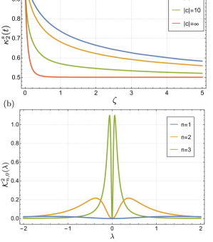
Figure 4: (a): The scaled second cumulant, $\kappa^{s}_{2}(t)$ of the attractive Lieb-Liniger model as a function of rescaled time $\zeta=t/\ell$ for $d=1$ and $|c|=1,2,10$. (b): the rapidity resolved cumulant, $\mathcal{K}^{2}_{n,0}(\lambda)$ for the first 3 quasi-particles as a function of $\lambda$ for $c=2$.

V FCS in the Gaudin-Yang model

We now consider the FCS in the Gaudin-Yang model, again splitting our analysis into two parts dealing with the repulsive and attractive regimes separately. In both cases the key component of our analysis, the overlap functions have been obtained previously by considering appropriate limits of the integrable quenches in the Hubbard model [91, 92].

V.1 Attractive interactions

We start by considering the attractive regime and taking into account the quasi-particle content of the model reviewed in Sec. III.2 we find

$$C^{s}_{\text{GGE}}(\beta)=\!\int\!\!{\rm d}\lambda\,\rho^{t}\!\left[\log\!\left(\frac{1+\zeta^{-1}_{\beta}}{{1+\zeta^{-1}_{0}}}\right)\!+\vartheta\log\frac{\zeta_{\beta}e^{\beta}}{\zeta_{0}}\right]\quad\quad\quad\quad$$

$$+\!\sum_{n=1}^{\infty}\!\int{\rm d}\lambda\,\sigma^{t}_{n}\!\left[\log\left(\frac{1+\eta^{-1}_{n,\beta}}{{1+\eta^{-1}_{n,0}}}\right)+\vartheta_{n}\log\frac{\eta_{n,\beta}}{\eta_{n,0}}\right]$$

$$+\int\!\!{\rm d}\lambda\,\tilde{\rho}^{t}\!\left[\log\left(\frac{1+\tilde{\zeta}^{-1}_{\beta}}{{1+\tilde{\zeta}^{-1}_{0}}}\right)+\vartheta\log\frac{\tilde{\zeta}_{\beta}e^{2\beta}}{\tilde{\zeta}_{0}}\right],\quad\quad$$ (64)

where the functions $\eta_{n,\beta},\zeta_{\beta},\tilde{\zeta}_{\beta}$ satisfy the integral equations

$$\log\eta_{n,\beta} = \log\!\left[\tanh^{2}\left(\frac{\pi\lambda}{2c}\right)\!\right]\!-\delta_{n,1}s\!*\!\log[1+\zeta^{-1}_{\beta}]$$ (65)

$$+s\!*\!\log[1+\eta_{n+1,\beta}][1+\eta_{n-1,\beta}]$$

$$\log\zeta_{\beta} = \log\!\left[\coth^{2}\left(\frac{\pi\lambda}{2c}\right)\!\right]\!+s\!*\!\log\left[\frac{1+\tilde{\zeta}_{\beta}}{1+\eta_{1,\beta}}\right]$$ (66)

$$\log\tilde{\zeta}_{\beta} = \log\left[\frac{\lambda^{4}(\lambda^{2}+c^{2})}{(2d)^{4}e^{2\beta}(\lambda^{2}+(c/2)^{2})}\right]+a_{1}\!*\!\log[1+\zeta^{-1}_{\beta}]$$ (67)

$$+a_{2}\!*\!\log[1+\tilde{\zeta}_{\beta}^{-1}].$$

Unlike in the LL model these equations do not admit an analytic solution that we are aware of and so must be treated numerically. There are however two limiting cases of interest. The first is the non-interacting limit $c\to 0^{-}$ in which case the dependence on the $\eta_{n,\beta}$ functions drop out and we find [10] $\zeta_{\beta}^{-1}=(1+\tilde{\zeta}^{-1}_{\beta})^{2}-1=e^{\beta}(2d)^{2}/\lambda^{2}$. As a result

$$C^{s}_{0}(\beta)|_{c\to 0^{-}}=\int\frac{{\rm d}\lambda}{2\pi}\log\left[\frac{\lambda^{2}+4d^{2}e^{2\beta}}{\lambda^{2}+4d^{2}}\right]=2d(e^{\beta}-1)\,,$$ (68)

for $\beta\in\mathbb{R}$, which is the SCGF of the Possion distribution with rate $2d$ and is therefore twice the result we found in the Tonks-Girardeau limit of the LL model (54). Accordingly we immediately find that the cumulants are $\kappa^{s}_{m}(0)=2d$ where we recall that the total fermionic density is $2d$. Additionally, the model has a second analytically tractable limit of interest, $|c|\to-\infty$. In this case not only do $\eta_{n,\beta}$ not contribute but now neither does $\zeta_{\beta}$ and the FCS are determined solely by the $2$-fermion bound states. This results from the fact that in the strongly attractive limit the fermion pairs in the initial state which make up $c^{\dagger}_{0}$ form bound states which cannot be broken apart . Thus the long time steady state consists only of these quasi-particles and no others. For this we find $\tilde{\zeta}_{\beta}=e^{-2\beta}\lambda^{4}/4d^{4}$ and the corresponding initial state FCS are

$$C^{s}_{0}(\beta)|_{c\to-\infty}=\int\frac{{\rm d}\lambda}{2\pi}\log\left[\frac{\lambda^{4}+4d^{4}e^{4\beta}}{\lambda^{4}+4d^{4}}\right]=2d(e^{\beta}-1)\,,$$ (69)

for $\beta\in\mathbb{R}$, i.e., the same result as in the free fermion limit, namely the SCGF of the Poisson distribution.

In these two limits the SCGF can similarly be computed at the steady-states, namely we have

$$C^{s}_{\text{GGE}}(\beta)|_{c\to 0^{-}}=\int\!\frac{{\rm d}\lambda}{\pi}\log\!\left[\frac{\lambda^{2}+4d^{2}e^{\beta}}{\lambda^{2}+4d^{2}}\right]\!=4d(e^{\beta/2}-1)\,,$$ (70)

and

$$C^{s}_{\text{GGE}}(\beta)|_{c\to-\infty}=\!\int\!\frac{{\rm d}\lambda}{\pi}\log\!\left[\frac{\lambda^{4}+4d^{4}e^{2\beta}}{\lambda^{4}+4d^{4}}\right]\!\!=\!4d(e^{\beta/2}\!-1)\,,$$ (71)

for $\beta\in\mathbb{R}$, which equal the SCGF of the LL model at infinite repulsion upon the substitution $d\rightarrow 2d$.

To investigate the cumulants at finite interaction we numerically integrate the equations (65)-(67) which requires that we truncate the number of strings which are included i.e. $\eta_{n,\beta}(\lambda),\sigma_{n}(\lambda)=0,\forall n>N_{\rm string}$ and also that we impose a cutoff on the allowed rapidities, $|\lambda|\leq\Lambda$. Doing so we can confirm that the cumulants of the steady state in fact do not depend on the interaction strength. Similarly to the case of the LL model, this implies that (64) yields $4d(e^{\beta/2}-1)$ with $d$ denoting the density of fermions, which can be confirmed numerically.

Finally, the full time evolution of the cumulants in the non-interacting limit can then be found using the previously result of (56) and similarly for $c\to-\infty$ whereas at finite $c$ we again resort to numerical integration of the TBA system. In Fig. 5 we plot the second cumulant as a function of time for different interaction strength. Here we note note that in contrast to the LL model the initial state is never an eigenstate of the model and so regardless of interaction strength the cumulant relaxes at finite scaled time. Nevertheless, the approach to the GGE value still depends upon the interaction strength with the different dynamics being attributed to the changing role of the quasi-particles. Specifically for large negative interaction the two particle bound states are dominant and as shown in Fig. 5 their contribution is peaked nearer the slower quasi-particles leading to an almost linear initial decrease. As the interaction strength is lowered the unbound particles also start to contribute and their mode resolved cumulant is more spread in rapidity space leading to a faster initial decay. The string contribution is negligible in all cases.

V.2 Repulsive interactions

As a final example we look at the repulsive GY model. In this regime the spectrum of the model does not include the two particle bound states and we have that

$$C^{s}_{\text{GGE}}(\beta)=\!\int\!\!{\rm d}\lambda\,\rho^{t}\!\left[\log\left(\frac{1+\zeta^{-1}_{\beta}}{{1+\zeta^{-1}_{0}}}\right)+\vartheta\log\frac{\zeta_{\beta}e^{\beta}}{\zeta_{0}}\right]\quad\quad\quad\quad$$

$$+\sum_{n=1}^{\infty}\int{\rm d}\lambda\,\sigma^{t}_{n}\!\left[\log\left(\frac{1+\eta^{-1}_{n,\beta}}{{1+\eta^{-1}_{n,0}}}\right)+\vartheta_{n}\log\frac{\eta_{n,\beta}}{\eta_{n,0}}\right]$$ (72)

where the functions $\eta_{n,\beta}$ and $\zeta_{\beta}$ satisfy a set of integral equations of the form (24). After using some standard TBA identities we find [10]

$$\log\eta_{n,\beta} = \log\!\left[\tanh^{2}\left(\frac{\pi\lambda}{2c}\right)\!\right]\!-\delta_{n,1}s\!*\!\log[1+\zeta^{-1}_{\beta}]$$ (73)

$$+s\!*\!\log[1+\eta_{n+1,\beta}][1+\eta_{n-1,\beta}]$$

$$\log\zeta_{\beta} = \log\!\left[\frac{\lambda^{2}+(c/2)^{2}}{\lambda^{2}e^{\beta}}\right]-\mu_{c}+s\!*\!\log[\lambda^{2}(\lambda^{2}+(c/2)^{2})]$$ (74)

$$+s\!*\!\log[1+\eta_{1,\beta}]+s\!*\!a_{1}\!*\!\log[1+\zeta^{-1}_{\beta}].$$

where $\mu_{c}$ is a Lagrange multiplier, introduced to fix the average density to be $2d$ and which behaves as $\lim_{c\to 0}\mu_{c}/c^{2}=2d^{2}$. As in the attractive case we cannot find an analytic solution to these equations however we can again consider the non-interacting limit $c\to 0^{+}$. In this limit the dependence on the $\eta_{n,\beta}$ functions drop out and $1+\zeta^{-1}_{\beta}=[1+\frac{4d^{2}}{\lambda^{2}}e^{\beta}]^{2}$ [10]. From this we then find that

$$C^{s}_{0}(\beta)|_{c\to 0^{+}}=\int\frac{{\rm d}\lambda}{2\pi}\log\left[\frac{\lambda^{2}+4d^{2}e^{2\beta}}{\lambda^{2}+4d^{2}}\right]$$ (75)

which agrees with the expression obtained from the (68). Thus the non-interacting limit of the FCS approached from both the repulsive and attractive sides agree.

Unlike the attractive case the opposite limit of $c\to\infty$ presents some problems. Indeed, exactly in this limit the initial state does not appear in the Hilbert space of the Hamiltonian since it precludes the possibility of two fermions being at the same position. By considering a lattice regularization of the model and taking the limit of infinite repulsion prior to the continuum limit it can be shown that the distribution functions become constants [91]. Consequently, in the repulsive GY model, as one increases the interaction strength the distribution $\rho(\lambda)$ becomes more and more spread in rapidity space. In the absence of an analytic solution to (73) and (74) must be treated numerically by first imposing some cutoff on both the string number and the rapidity space as was done in the attractive regime. However, the aforementioned spreading in rapidity space of the distributions results in a strong dependence on these truncation schemes leading to unreliable data except at small $c$ where the results are qualitatively the same as the non-interacting limit. Despite this however, we expect that the relationship between the cumulants remains valid.

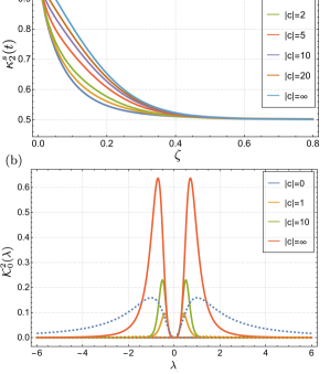
Figure 5: (a): The scaled second cumulant, $\kappa^{s}_{2}(t)$ as a function of the scaled time $\zeta=t/\ell$ for different values of the interactions strength in the attractive regime. (b): The rapidity resolved second cumulant for the two particle bound states (solid lines), $\tilde{\mathcal{K}}^{2}_{0}(\lambda)$ as a function of $\lambda$ for different interaction strengths. Also shown are rapidity resolved second cumulant for the unbound states (dashed lines), $\mathcal{K}^{2}_{0}(\lambda)$. In the $c=0^{-}$ case only unbound states are present while in the opposite limit $|c|\to\infty$ only bound states are present. For any finite interaction the unbound states are strongly suppressed and not discernible on the same scale.

VI Charge Probability distributions

In the previous sections we demonstrated that the scaled cumulants of charge fluctuations in the steady-state are universal for BEC quenches in both the LL and GY models. That is, they do not depend on the interaction strength of these quantum gases and they are determined by scaled cumulants in the initial states, which are essentially identical in both models. We now address the characterization of the full charge probability distribution in the steady state of the LL model and in the initial and steady-states of the GY model. The standard and mathematically precise way of achieving this task is using the Gärtner-Ellis theorem and eventually computing the Legendre-Fenchel transform of the SCGF and using Eq. (7). During the previous analysis, nevertheless, we also argued that the SCGF in the steady-states of the LL and GY models can be written by the analytic function

$$C^{s}_{\text{GGE}}(\beta)=C^{s}_{\text{an}}(\beta)=\sum_{m=1}^{\infty}\frac{\kappa^{s}_{m}\beta^{m}}{m!}=2d(e^{\beta/2}-1)\,,$$ (76)

independently of the interaction strengths, and where the density $d$ denotes the density of bosons or the ’quasi-bosons’ in the initial states of the LL and GY models, respectively. In fact, $C^{s}_{\text{an}}$ equals Eq. (55), that is the $C^{s}_{\text{GGE}}(\beta)|_{c\to\infty}$ expression explicitly computed from the QA equations in the LL model. Similarly, $C^{s}_{\text{an}}(\beta)$ equals (70) as well as (71) (that is the $C^{s}_{\text{GGE}}(\beta)|_{c\to 0^{-}}$ and the $C^{s}_{\text{GGE}}(\beta)|_{c\to-\infty}$ limits in the GY model) apart from a factor of two, which further underpin the validity of $C^{s}_{\text{an}}(\beta)$ and Eqs. (76) at arbitrary interactions. Finally we note that the numerical solutions for the SCGF originating from the QA equations also confirm (76).

Given the explicit analytic expression for the SCGF of the steady-states, and focusing first on the LL model, the rate function $I(z)$ can be easily obtained, namely

$$I(z)=(2d-2z+2z\log(z/d))$$ (77)

i.e., twice the rate function of the Poisson distribution and thus $P(\ell z)$ has non-trivial and non-Gaussian fluctuations and large deviations. The rate function unambiguously characterises the limiting coarse-grained PD $P(\ell z,0)$ in the asymptotic sense (cf. (8)).

Nevertheless, as we have anticipated, it is also instructive to approximate the steady-state PD by using

$$P(n)\approx\int_{-\pi}^{\pi}\frac{{\rm d}\beta}{2\pi}e^{-i\beta n}e^{\ell C^{s}(i\beta)}$$ (78)

that is by neglecting the $o(\ell)$ terms in the (2nd) cumulant generating function. To use (78) the knowledge of the second SCGF is required, but given the analytic nature of (76), we can invoke that

$$C^{s}_{\text{an}}(i\beta)=2d(e^{i\beta/2}-1)\,.$$ (79)

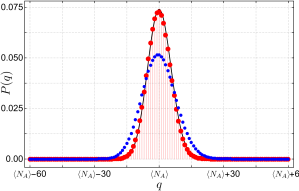
Figure 6: The probability distributions (red dots and black line) of charge fluctuations in the steady state of the LL model after a BEC quench in a large but finite subsystem. The red dots were obtained using Eq. (78) whereas the black continuous line corresponds to the rescaled limiting PD obtained from the rate function (77). The blue dots show the Poisson PD of the initial state. The subsystem size $\ell$ equals 60 and the particle density is unity $d=1$.

In Fig. 6 we display the rescaled limiting probability distribution $P(z)\asymp\text{const}\times e^{-\ell I(z/\ell)}$ obtained from the rate function and the discrete probabilities resulting from (78) to demonstrate their agreement. It is important to stress, that although the PDs look Gaussian, this is not the case, since the cumulants and the asymptotics of the PDs are markedly different. One main feature that can be observed is that the variance of the PD in the steady-state is $1/\sqrt{2}$ times that of the initial state, or in other words, the distribution gets squeezed during the time evolution.

A remark can be made in connection with approximating the steady-state PD of a large but finite system via (78). Notably, the Fourier integral can be analytically computed resulting in lengthy expressions of trigonometric functions and exponential integrals. However, due to these expressions it is easy to show that $C^{s}_{\text{an}}(i\beta)$ does not define a PD in the strict sense, as for small $\ell$ negative probabilities can occur. Nevertheless increasing $\ell$, as expected, the probabilities become positive numbers sum up to one and the discrete probabilities also reproduce the predicted results for the cumulants, which we have checked explicitly focusing on the first four.

We now turn to the discussion of the PDs in the GY model and first consider the PD in the initial state. Similarly to the LL model, the scaled cumulants in the initial states are constant, that is, $\kappa^{s}_{m}(0)=2d$, where $d$ in this case is the density of fermion pairs. In the infinite subsystem size limit, the limiting continuous PD is therefore described by the rate function of the Poissonian, i.e., $I_{0}(z)=2d-z+z\log(z/(2d))$. Nevertheless, the microscopic, discrete PD is anticipated to be different from a Poissonian, due the vanishing probabilities of odd particle numbers. Surprisingly, directly computing the 2nd SCGF at the free fermion limit using explicitly the integral in (68) at imaginary $\beta$ reveals how such a microscopic effect can manifest. The 2nd SCGF obtained this way, denoted by $C^{s}_{0,GY}$, is a non-analytic function, equals $2d(e^{i\beta}-1)$ in the $[-\pi/2,\pi/2]$ interval, and outside this interval it is defined by the relations $C^{s}_{0,GY}(i\pi-i\beta)=C^{s}_{0,GY}(i\beta)^{*}$ and $C^{s}_{0,GY}(-i\pi+i\beta)=C^{s}_{0,GY}(-i\beta)^{*}$, which are the consequence of a particular choice for the branches of the logarithm. Nevertheless, these symmetry properties ensure that the Fourier integrals (78) vanish for every odd number. The integrals can again be explicitly evaluated in terms of analytic expressions and hence it can be checked that for large enough subsystems, the probabilities are positive, sum up to one and the scaled cumulants match the expected value $2d$. We again stress that such a microscopic effect shall not affect the limiting and continuous PD $P(\ell z,0)$, however in large but finite subsystems, this feature is anticipated to be present and the corresponding discrete PD is assumed to be well approximated by $C^{s}_{0,GY}(i\beta)$ via (78).

Finally, we discuss the charge probabilities in steady-state of the GY model after the BEC quench. Our main focus again concerns some microscopic features of a discrete charge distribution in a finite subsystem, and in the infinite subsystem limit we assume to recover $P(\ell z,\infty)\asymp e^{-\ell I(z)}$ where $I(z)$ equals (77) upon the $d\rightarrow 2d$ substitution.

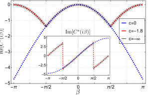
Figure 7: The real and imaginary (inset) part of the 2nd scaled cumulant generating functions $C^{s}(i\beta)$ in the steady-state of the Gaudin-Yang model with a fixed density $d=2.4$ and various interaction strengths. The functions are obtained from the solution of the QA equations and performing numerical integration ($c=-1.8$) or using exact expression for the integral (19) ($c=0$ and $c\rightarrow-\infty$). The function for $c=0$ coincides with $C^{s}_{\text{an}}(i\beta)$, i.e., the analytic function defined by a Taylor series via the cumulants.

We first take a look at the 2nd SCGFs originating from the QA equations and plot these functions in Fig. 7. Based on the figure it can be seen that in the $c\rightarrow 0^{-}$, i.e., the free fermion limit, the analytically computed function $C^{s}(i\beta)$ obtained from the integral in Eq. (70) performing the $\beta\rightarrow i\beta$ substitution equals $C^{s}_{\text{an}}$. Nevertheless, for non-zero interaction strengths we obtain collapsing non analytic functions. This function can be computed using the integral in (71) after substituting $\beta$ with $i\beta$. The function $C^{s}_{\infty,GY}$ one obtains this way equals $4d(e^{i\beta/2}-1)$ in the $[-\pi/2,\pi/2]$ interval, and outside this interval it is given by the properties $C^{s}_{\infty,GY}(i\pi-i\beta)=C^{s}_{\infty,GY}(i\beta)^{*}$ and $C^{s}_{\infty,GY}(-i\pi+i\beta)=C^{s}_{\infty,GY}(-i\beta)^{*}$. Although the non-analytic behaviour may again be attributed to the improper treatment of the branches of the logarithm, interestingly, together with the symmetry properties of the function they give some insight into a microscopic physical effect, although less obvious in this case. Similarly to the fermionic BEC state, the non-analytic 2nd SCGF with the particular symmetry properties imply vanishing probabilities for odd fermion numbers, when the charge fluctuations in large but finite subsystem are considered via (78). Importantly, this feature is expected to take place in the $c\rightarrow-\infty$ limit, as in this case, only the fermion, spin-singlet bound states have non-vanishing densities in the steady-state. That is, the unit charge is two, hence probabilities for odd numbers must vanish . Similarly to the previous cases, the Fourier integral (78) involving $C^{s}_{\infty,GY}$ can be computed analytically and when the subsystem size $\ell$ is large, the PD consists of positive probabilities summing up to one, and increasing $\ell$ the scaled cumulants converge to the prescribed value $\kappa_{m}^{s}(\infty)=2d/2^{m-1}$ as we have explicitly checked for the first four cumulants.

The situation is less understood at finite interaction strengths in the attractive regime. Although the numerically obtained 2nd SCGFs collapse to $C^{s}_{\infty,GY}(i\beta)$, in this case it is not clear whether or not the symmetry properties of the 2nd SCGF can be associated with a microscopic effect. Namely, it is not obvious why the probabilities for observing an odd number of particles in a subsystem should be zero, since at finite $c$, the root densities for the species associated with charge 1 are non-vanishing. Their contribution to the cumulants is, however, strongly suppressed for any non-zero interaction (see Fig. 5) and so it is possible that in the thermodynamic limit the odd probabilities are vanishing. Unfortunately this question cannot be definitively answered within the framework of the QA techniques we are using, therefore we leave it open for further investigations. In the repulsive regime of the model, however, we do not anticipate ambiguities and the presence of such microscopic effects due the lack of fermion bound states.

To conclude this section, we again wish to stress that by our methods we are able to give precise predictions for the continuous limiting PD $P(\ell z)$ via the rate function $I(z)$ for all the non-trivial cases, that is for the steady-state of the LL and the GY model. Going beyond the continuous description of the limiting PD, or, eventually the $\ell\rightarrow\infty$ limit, is nevertheless out of the range of the methods we have. It is therefore quite surprising, that the 2nd SCGF computed from the QA method could give hints about certain microscopic features, which are clearly beyond the scaling limit $\ell\rightarrow\infty$. In particular, the emergent and uncontrolled non-analytic behaviour correctly indicate microscopic structures in the fermionic BEC initial states as well as in the steady-state of the GY model at infinite attraction, which manifest in vanishing probabilities for odd charges in finite but large subsystems. The indications of the 2nd SCGFs are always to be reconciled with additional physical considerations, which nevertheless are lacking at the moment for the case of the steady-state fluctuations of the GY model at finite attractive interactions.

VII Conclusions

In this paper we analyzed out-of-equilibrium charge fluctuations in two paradigmatic models of one dimensional quantum gases. In particular, we investigated the Lieb-Liniger model which describes interacting bosonic particles, and the Gaudin-Yang model in which the interacting particles are fermions and explored their entire parameter space by considering generic repulsive and attractive interactions. We focused on two particular initial states, the Bose-Einstein condensate state and its fermionic analog for the Lieb-Liniger and Gaudin-Yang models, respectively. These choices allowed for a rather complete characterization of non-trivial charge fluctuations over the course of the entire time evolution. This achievement is due the applicability of powerful methods relying on the integrability of the physical systems and the peculiar structure of the initial states.

In particular, using novel analytical techniques [55, 56, 64] and inspired by the quench action method [11], we determined all the scaled cumulants of charge fluctuations in the steady state as well their time evolution. These quantities characterize the fluctuations in a very large subsystem by keeping the leading order (linear in subsystem size) behavior. Whereas the time evolution of the scaled cumulants generically depends on the interaction strength of the models, surprisingly, their value in the steady-state was found to be independent of it. Moreover, it was also revealed that the scaled cumulants in the steady-state are uniquely characterised by the corresponding scaled cumulants in the initial state in a remarkably simple fashion. In particular, the scaled cumulants $\kappa^{s}_{m}(0)$ in both the conventional and the fermionic BEC states are $\kappa^{s}_{m}(0)=d$ and $\kappa^{s}_{m}(0)=2d$, respectively, where $d$ is the density of bosons and fermion pairs in the two states. In the steady-states the scaled cumulants $\kappa^{s}_{m}(\infty)$ are instead given by the universal relation $\kappa^{s}_{m}(\infty)=\kappa^{s}_{m}(0)/2^{m-1}$. This relation was established based on the explicit determination of the scaled cumulants in the initial and steady-states. A formal derivation of this relationship was also provided based on comparing the full counting statistics in the diagonal ensemble and in the generalized Gibbs ensemble and by showing that the former can capture the fluctuations in the initial state.

Thanks to the exponential decay of the scaled cumulants in the steady-states we could naturally invoke the scaled cumulant generating function whose determination based on only the knowledge of the cumulants, in general, might not be straightforward. Nevertheless, the analytic function obtained this way also agrees the generating functions obtained directly from the quench action method at specific interaction strength, when analytic computations are feasible or at generic interaction strengths, when the agreement can be checked numerically. Computing the Legendre-Fenchel transform of this function we obtained an explicit expression for the rate function which characterizes the limiting continuous probability distribution in an infinitely large subsystem. In accordance with the scaled cumulants in the steady-state, this function predicts non-trivial and non-Gaussian fluctuations and large deviations for the charge. Additionally, we also considered the probability distributions in large but finite subsystems, where their discrete nature is still visible. An interesting feature occurs in the fermionic BEC initial state as well as in the steady-state of the Gaudin-Yang model at infinite attraction. In these cases the probabilities of observing an odd number of charge in a subsystem identically vanish. Nevertheless, resolving such discrete and microscopic features in strictly finite subsystems is beyond the scope of our current methods and hence was accomplished by relying on additional physical input.

Our work admits several pathways for further investigations. A surprising finding is the universal relationship between the scaled cumulants of the initial and steady-states, which is a consequence of the integrability of both the models and the initial states [94]. It would be important to identify the precise conditions for the onset of this phenomenon and to give a more rigorous explanation than what is presented in this work. A noteworthy remark is that, for initial states with vanishing scaled cumulants, such predictions clearly cannot hold. However, universality was manifest in our examples in another way as well, namely by the lack of dependence on the interaction strength of the models. It is an interesting question whether such interaction-independence can be observed in other, possibly non-integrable models or in other quench protocols, or it again requires the integrability of both the post-quench Hamiltonian and the initial state. Finally it would be worthwhile to accomplish the challenging task of developing analytic or semi-analytic methods that can capture the sub-leading behavior of fluctuations. This would be important to characterize certain microscopic effects, such as the fluctuations of conserved quantities in a subsystem for which the cumulants admit sub-extensive scaling e.g. those associated with the KPZ universality class [95].

Appendix A A formal derivation of the SCGF of the initial state from the diagonal ensemble

A main finding of this manuscript is the simple relationship between the scaled cumulants of the initial and the steady-states. This reads as $\kappa_{m}^{s}(\infty)=\kappa_{m}^{s}(0)/2^{m-1}$ or when promoted onto the level of the scaled cumulant generating functions, $C^{s}_{0}(\beta)=2C^{s}_{\text{GGE}}(\beta/2)$. These relations were obtained by comparing the FCS in the diagonal ensemble (DE) and in the GGE of the quench problem in Sec. II and were justified in the following subsections by explicitly computing the corresponding cumulants in the initial/stead-states. While our explanation for these relationships at its present form shall remain formal, in this appendix we intend to comment more on the non-trivial bit therein, namely why and how the diagonal ensemble can describe the FCS in the initial and not in the steady-state.

First of all, let us recall the result of Ref. [64], which claims that in a (G)GE, the SCGF of a conserved charge can be obtained by

$$C^{s}_{\text{GGE}}(\beta)=f_{\text{GGE}}(\underline{\beta}^{(k)}+\beta)-f_{\text{GGE}}(\underline{\beta}^{(k)})$$ (80)

where $f_{\text{GGE}}$ denotes the free energy density of a GGE characterized by the chemical potentials $\underline{\beta}^{(k)}$ and $\beta$ is associated with the particular conserved quantity of interest. We shall use this relation as a guideline in what follows. Let us now specify the FCS in the initial state denoted by $|\Psi_{0}\rangle$

$$\langle\Psi_{0}|e^{\beta\hat{N}_{A}}|\Psi_{0}\rangle=\frac{1}{\langle\Psi_{0}|\Psi_{0}\rangle}\sum_{\Phi,\Phi^{\prime}}e^{-\epsilon_{\Phi}^{*}-\epsilon_{\Phi^{\prime}}}\langle\Phi|e^{\beta\hat{N}_{A}}|\Phi^{\prime}\rangle\,,$$ (81)

where $A$ denotes the subsystem whose length is $\ell$, $\epsilon_{\Phi}=-\log{\innerproduct{\Phi}{\Psi_{0}}}$ are the logarithmic overlaps and in Eq. (81) we merely expanded the initial state in the eigenbasis of the post-quench Hamiltonian. For simplicity and transparency, we assume only one particle species. Following the logic of the QA method, we can replace one summation by a functional integral over root distributions assuming that the size of the entire system $L$ is very large and is eventually sent to infinity. This way we may write

$$\langle\Psi_{0}|e^{\beta\hat{N}_{A}}|\Psi_{0}\rangle=\sum_{\Phi}\!\int\!\mathcal{D}[\rho]e^{S_{YY}[\rho]}\!\left[e^{-\epsilon_{\Phi}^{*}-\epsilon[\rho]}\langle\Phi|e^{\beta\hat{N}_{A}}|\rho\rangle\right.$$

$$+\left.\Phi\leftrightarrow\rho\vphantom{\frac{OOOOO}{OOOOO}}\right]\times\frac{1}{\langle\Psi_{0}|\Psi_{0}\rangle},\quad\quad\quad$$ (82)

where $S_{YY}$ the Yang-Yang entropy of the root distribution whose exponential gives the number of microstates with the same root distribution. Note that the up to this point we have two length scales, $\ell$ associated with the length of the subsystem and $L$ with the total length of the system. The essential next step is the following: we extend the support of the subsystem $A$ and consider the charge operator in the entire system. This is formal step since when $L=\ell$ no charge fluctuations are expected. The step is rather based on the analogy with the treatment of FCS, more precisely the SCGF in GGEs. Namely one can relate the SCGF of a very large subsystem ($\ell\rightarrow\infty$) with free energy densities in which the conserved quantity is regarded in the entire system. Performing this extension, it can immediately be seen that we can get rid of the second summation, since $\langle\Phi|e^{\beta\hat{N}}|\rho\rangle$ is a conserved quantity and can have only diagonal matrix elements. That is, we can rewrite Eq. (82) as

$$\langle\Psi_{0}|e^{\beta\hat{N}}|\Psi_{0}\rangle=\frac{1}{\langle\Psi_{0}|\Psi_{0}\rangle}\int\mathcal{D}[\rho]e^{S_{YY}[\rho]-2\text{Re}\epsilon[\rho]}\langle\rho|e^{\beta\hat{N}}|\rho\rangle$$ (83)

where we keep in mind that we changed the way of sending $L$ and $\ell$ to infinity by essentially equating these lengths. This expression can be further rewritten as

$$\begin{split}\langle\Psi_{0}|e^{\beta\hat{N}}|\Psi_{0}\rangle=&\int\mathcal{D}[\rho]e^{S_{YY}[\rho]-2\text{Re}\,\epsilon[\rho]+\ell\int\text{d}\lambda\beta q\rho(\lambda)}\\ &\times\left[\int\mathcal{D}[\rho]e^{S_{YY}[\rho]-2\text{Re}\,\epsilon[\rho]}\right]^{-1}\,,\end{split}$$ (84)

which is equivalent to Eq. (22), if the pair-structure of the initial state is imposed. Using the saddle point approximation and taking the logarithm of (84) we can write down the SCGF as a difference of two effective free energy densities, i.e.,

$$\begin{split}\log\langle&\Psi_{0}|e^{\beta\hat{N}}|\Psi_{0}\rangle=\ell C^{s}_{0}(\beta)+o(\ell)\\ &=-\frac{\ell}{2}\int\text{d}\lambda\left(g(\lambda)-2\beta q)\bar{\rho}_{sp}(\lambda)\right)-\frac{1}{2}S_{YY}[\bar{\rho}_{sp}]\\ &+\frac{\ell}{2}\int\text{d}\lambda g(\lambda)\rho)_{sp}(\lambda+\frac{1}{2}S_{YY}[\rho_{sp}]+o(\ell)\,,\end{split}$$ (85)

where adapted the notation of the logarithmic overlaps from Sec. II, took into account the $1/2$ factors due to the pair-structure of the initial state, and $\bar{\rho}_{sp}$ and $\rho_{sp}$ are the two saddle-point root distributions of the nominator and the denominator of (84).

References

- Polkovnikov et al. [2011] A. Polkovnikov, K. Sengupta, A. Silva, and M. Vengalattore, Colloquium: Nonequilibrium dynamics of closed interacting quantum systems, Rev. Mod. Phys. 83, 863 (2011).
- Calabrese et al. [2016] P. Calabrese, F. H. Essler, and G. Mussardo, Introduction to “Quantum integrability in out of equilibrium systems”, J. Stat. Mech. 2016, 064001 (2016).
- Vidmar and Rigol [2016] L. Vidmar and M. Rigol, Generalized Gibbs ensemble in integrable lattice models, J. Stat. Mech. 2016, 064007 (2016).
- Essler and Fagotti [2016] F. H. L. Essler and M. Fagotti, Quench dynamics and relaxation in isolated integrable quantum spin chains, J. Stat. Mech. 2016, 064002 (2016).
- Doyon [2020] B. Doyon, Lecture notes on generalised hydrodynamics, SciPost Phys. Lect. Notes , 18 (2020).
- Bastianello et al. [2022] A. Bastianello, B. Bertini, B. Doyon, and R. Vasseur, Introduction to the special issue on emergent hydrodynamics in integrable many-body systems, J. Stat. Mech. 2022, 014001 (2022).
- Alba et al. [2021] V. Alba, B. Bertini, M. Fagotti, L. Piroli, and P. Ruggiero, Generalized-hydrodynamic approach to inhomogeneous quenches: correlations, entanglement and quantum effects, J. Stat. Mech. 2021, 114004 (2021).
- Rylands and Andrei [2020] C. Rylands and N. Andrei, Nonequilibrium aspects of integrable models, Annual Review of Condensed Matter Physics 11, 147 (2020).
- Korepin et al. [1993] V. E. Korepin, N. M. Bogoliubov, and A. G. Izergin, Quantum Inverse Scattering Method and Correlation Functions, Cambridge Monographs on Mathematical Physics (Cambridge University Press, 1993).
- Takahashi [1999] M. Takahashi, Thermodynamics of One-Dimensional Solvable Models (Cambridge University Press, 1999).
- Caux and Essler [2013] J.-S. Caux and F. H. L. Essler, Time evolution of local observables after quenching to an integrable model, Phys. Rev. Lett. 110, 257203 (2013).
- Caux [2016] J.-S. Caux, The quench action, J. Stat. Mech.: Theory Exp. 2016 (6), 064006.
- Castro-Alvaredo et al. [2016] O. A. Castro-Alvaredo, B. Doyon, and T. Yoshimura, Emergent hydrodynamics in integrable quantum systems out of equilibrium, Phys. Rev. X 6, 041065 (2016).
- Bertini et al. [2016] B. Bertini, M. Collura, J. De Nardis, and M. Fagotti, Transport in out-of-equilibrium XXZ chains: Exact profiles of charges and currents, Phys. Rev. Lett. 117, 207201 (2016).
- Doyon et al. [2023a] B. Doyon, G. Perfetto, T. Sasamoto, and T. Yoshimura, Emergence of hydrodynamic spatial long-range correlations in nonequilibrium many-body systems, Phys. Rev. Lett. 131, 027101 (2023a).
- Bloch et al. [2008] I. Bloch, J. Dalibard, and W. Zwerger, Many-body physics with ultracold gases, Rev. Mod. Phys. 80, 885 (2008).
- Cazalilla et al. [2011] M. A. Cazalilla, R. Citro, T. Giamarchi, E. Orignac, and M. Rigol, One dimensional bosons: From condensed matter systems to ultracold gases, Rev. Mod. Phys. 83, 1405 (2011).
- Guan et al. [2013] X.-W. Guan, M. T. Batchelor, and C. Lee, Fermi gases in one dimension: From bethe ansatz to experiments, Rev. Mod. Phys. 85, 1633 (2013).
- Lieb and Robinson [1972] E. H. Lieb and D. W. Robinson, The finite group velocity of quantum spin systems, in Statistical mechanics, edited by B. Nachtergaele, J. P. Solovej, and J. Yngvason (Springer, 1972) pp. 425–431.
- Yang [1967] C. N. Yang, Some exact results for the many-body problem in one dimension with repulsive delta-function interaction, Phys. Rev. Lett. 19, 1312 (1967).
- Gaudin [1967] M. Gaudin, Un systeme a une dimension de fermions en interaction, Physics Letters A 24, 55 (1967).
- Zamolodchikov and Zamolodchikov [1979] A. B. Zamolodchikov and A. B. Zamolodchikov, Factorized S-matrices in two dimensions as the exact solutions of certain relativistic quantum field theory models, Annals of Physics 120, 253 (1979).
- Kinoshita et al. [2006] T. Kinoshita, T. Wenger, and D. S. Weiss, A quantum Newton’s cradle, Nature (London) 440, 900 (2006).
- Gritsev et al. [2007a] V. Gritsev, E. Demler, M. Lukin, and A. Polkovnikov, Spectroscopy of collective excitations in interacting low-dimensional many-body systems using quench dynamics, Phys. Rev. Lett. 99, 200404 (2007a).
- Gritsev et al. [2007b] V. Gritsev, A. Polkovnikov, and E. Demler, Linear response theory for a pair of coupled one-dimensional condensates of interacting atoms, Phys. Rev. B 75, 174511 (2007b).
- Pigneur et al. [2018] M. Pigneur, T. Berrada, M. Bonneau, T. Schumm, E. Demler, and J. Schmiedmayer, Relaxation to a phase-locked equilibrium state in a one-dimensional bosonic josephson junction, Phys. Rev. Lett. 120, 173601 (2018).
- Zache et al. [2020] T. V. Zache, T. Schweigler, S. Erne, J. Schmiedmayer, and J. Berges, Extracting the field theory description of a quantum many-body system from experimental data, Phys. Rev. X 10, 011020 (2020).
- Roy and Saleur [2019] A. Roy and H. Saleur, Quantum electronic circuit simulation of generalized sine-gordon models, Phys. Rev. B 100, 155425 (2019).
- Horváth et al. [2019] D. X. Horváth, I. Lovas, M. Kormos, G. Takács, and G. Zaránd, Nonequilibrium time evolution and rephasing in the quantum sine-Gordon model, Phys. Rev. A 100, 013613 (2019).
- Roy et al. [2021] A. Roy, D. Schuricht, J. Hauschild, F. Pollmann, and H. Saleur, The quantum sine-Gordon model with quantum circuits, Nuclear Physics B 968, 115445 (2021).
- Rylands et al. [2020] C. Rylands, Y. Guo, B. L. Lev, J. Keeling, and V. Galitski, Photon-mediated peierls transition of a 1d gas in a multimode optical cavity, Phys. Rev. Lett. 125, 010404 (2020).
- Horváth et al. [2022] D. X. Horváth, S. Sotiriadis, M. Kormos, and G. Takács, Inhomogeneous quantum quenches in the sine-Gordon theory, SciPost Phys. 12, 144 (2022).
- Bastianello [2023] A. Bastianello, The sine-Gordon model from coupled condensates: a generalized hydrodynamics viewpoint, arXiv:2310.04493 (2023).
- Senaratne et al. [2022] R. Senaratne, D. Cavazos-Cavazos, S. Wang, F. He, Y.-T. Chang, A. Kafle, H. Pu, X.-W. Guan, and R. G. Hulet, Spin-charge separation in a one-dimensional fermi gas with tunable interactions, Science 376, 1305–1308 (2022).
- Langen et al. [2015] T. Langen, S. Erne, R. Geiger, B. Rauer, T. Schweigler, M. Kuhnert, W. Rohringer, I. E. Mazets, T. Gasenzer, and J. Schmiedmayer, Experimental observation of a generalized Gibbs ensemble, Science 348, 207 (2015).
- Schemmer et al. [2019] M. Schemmer, I. Bouchoule, B. Doyon, and J. Dubail, Generalized hydrodynamics on an atom chip, Phys. Rev. Lett. 122, 090601 (2019).
- Malvania et al. [2021] N. Malvania, Y. Zhang, Y. Le, J. Dubail, M. Rigol, and D. S. Weiss, Generalized hydrodynamics in strongly interacting 1D Bose gases, Science 373, 1129 (2021).
- Le et al. [2023] Y. Le, Y. Zhang, S. Gopalakrishnan, M. Rigol, and D. S. Weiss, Observation of hydrodynamization and local prethermalization in 1d Bose gases, Nature 618, 494–499 (2023).
- Cherng and Demler [2007] R. W. Cherng and E. Demler, Quantum noise analysis of spin systems realized with cold atoms, New Journal of Physics 9, 7–7 (2007).
- Klich and Levitov [2009] I. Klich and L. Levitov, Quantum noise as an entanglement meter, Phys. Rev. Lett. 102, 100502 (2009).
- Eisler and Rácz [2013] V. Eisler and Z. Rácz, Full counting statistics in a propagating quantum front and random matrix spectra, Phys. Rev. Lett. 110, 060602 (2013).
- Eisler [2013] V. Eisler, Universality in the full counting statistics of trapped fermions, Phys. Rev. Lett. 111, 080402 (2013).
- Lovas et al. [2017] I. Lovas, B. Dóra, E. Demler, and G. Zaránd, Full counting statistics of time-of-flight images, Phys. Rev. A 95, 053621 (2017).
- Najafi and Rajabpour [2017] K. Najafi and M. A. Rajabpour, Full counting statistics of the subsystem energy for free fermions and quantum spin chains, Phys. Rev. B 96, 235109 (2017).
- Collura et al. [2017] M. Collura, F. H. L. Essler, and S. Groha, Full counting statistics in the spin-1/2 Heisenberg XXZ chain, J. Phys. A: Math. Theor. 50, 414002 (2017).
- Bastianello and Piroli [2018] A. Bastianello and L. Piroli, From the sinh-Gordon field theory to the one-dimensional Bose gas: exact local correlations and full counting statistics, J. Stat. Mech.: Theory Exp. 2018 (11), 113104.
- van Nieuwkerk and Essler [2019] Y. D. van Nieuwkerk and F. H. L. Essler, Self-consistent time-dependent harmonic approximation for the sine-gordon model out of equilibrium, Journal of Statistical Mechanics: Theory and Experiment 2019, 084012 (2019).
- Calabrese et al. [2020] P. Calabrese, M. Collura, G. D. Giulio, and S. Murciano, Full counting statistics in the gapped XXZ spin chain, EPL 129, 60007 (2020).
- Collura and Essler [2020] M. Collura and F. H. L. Essler, How order melts after quantum quenches, Phys. Rev. B 101, 041110 (2020).
- Doyon et al. [2023b] B. Doyon, G. Perfetto, T. Sasamoto, and T. Yoshimura, Ballistic macroscopic fluctuation theory, SciPost Phys. 15, 136 (2023b).
- Oshima and Fuji [2022] H. Oshima and Y. Fuji, Charge fluctuation and charge-resolved entanglement in monitored quantum circuit with symmetry, arXiv:2210.16009 (2022).
- Tartaglia et al. [2022] E. Tartaglia, P. Calabrese, and B. Bertini, Real-time evolution in the Hubbard model with infinite repulsion, SciPost Phys. 12, 028 (2022).
- Parez et al. [2021a] G. Parez, R. Bonsignori, and P. Calabrese, Quasiparticle dynamics of symmetry-resolved entanglement after a quench: Examples of conformal field theories and free fermions, Phys. Rev. B 103, L041104 (2021a).
- Parez et al. [2021b] G. Parez, R. Bonsignori, and P. Calabrese, Exact quench dynamics of symmetry resolved entanglement in a free fermion chain, J. Stat. Mech.: Theory Exp. 2021 (9), 093102.
- Bertini et al. [2023a] B. Bertini, P. Calabrese, M. Collura, K. Klobas, and C. Rylands, Nonequilibrium full counting statistics and symmetry-resolved entanglement from space-time duality, Phys. Rev. Lett. 131, 140401 (2023a).
- Bertini et al. [2023b] B. Bertini, K. Klobas, M. Collura, P. Calabrese, and C. Rylands, Dynamics of charge fluctuations from asymmetric initial states, arXiv:2306.12404 (2023b).
- Scopa and Horváth [2022] S. Scopa and D. X. Horváth, Exact hydrodynamic description of symmetry-resolved Rényi entropies after a quantum quench, Journal of Statistical Mechanics: Theory and Experiment 2022, 083104 (2022).
- Pálmai and Sotiriadis [2014] T. Pálmai and S. Sotiriadis, Quench echo and work statistics in integrable quantum field theories, Physical Review E 90, 10.1103/physreve.90.052102 (2014).
- Groha et al. [2018] S. Groha, F. H. L. Essler, and P. Calabrese, Full counting statistics in the transverse field Ising chain, SciPost Phys. 4, 043 (2018).
- Rylands and Andrei [2019a] C. Rylands and N. Andrei, Quantum work of an optical lattice, Phys. Rev. B 100, 064308 (2019a).
- Rylands and Andrei [2019b] C. Rylands and N. Andrei, Loschmidt amplitude and work distribution in quenches of the sine-Gordon model, Phys. Rev. B 99, 085133 (2019b).
- Perfetto et al. [2019] G. Perfetto, L. Piroli, and A. Gambassi, Quench action and large deviations: Work statistics in the one-dimensional Bose gas, Phys. Rev. E 100, 032114 (2019).
- Bastianello et al. [2018] A. Bastianello, L. Piroli, and P. Calabrese, Exact local correlations and full counting statistics for arbitrary states of the one-dimensional interacting Bose gas, Phys. Rev. Lett. 120, 190601 (2018).
- Doyon and Myers [2019] B. Doyon and J. Myers, Fluctuations in ballistic transport from euler hydrodynamics, Annales Henri Poincaré 21, 255–302 (2019).
- Myers et al. [2020] J. Myers, M. J. Bhaseen, R. J. Harris, and B. Doyon, Transport fluctuations in integrable models out of equilibrium, SciPost Phys. 8, 007 (2020).
- Gopalakrishnan et al. [2022] S. Gopalakrishnan, A. Morningstar, R. Vasseur, and V. Khemani, Theory of anomalous full counting statistics in anisotropic spin chains, arXiv:2203.09526 (2022).
- Krajnik et al. [2022a] Ž. Krajnik, J. Schmidt, V. Pasquier, E. Ilievski, and T. Prosen, Exact anomalous current fluctuations in a deterministic interacting model, Phys. Rev. Lett. 128, 160601 (2022a).
- Krajnik et al. [2022b] Ž. Krajnik, J. Schmidt, V. Pasquier, T. Prosen, and E. Ilievski, Universal anomalous fluctuations in charged single-file systems, arXiv:2208.01463 (2022b).
- Samajdar et al. [2023] R. Samajdar, E. McCulloch, V. Khemani, R. Vasseur, and S. Gopalakrishnan, Quantum turnstiles for robust measurement of full counting statistics, arXiv preprint arXiv:2305.15464 (2023).
- Krajnik et al. [2023] Ž. Krajnik, E. Ilievski, and T. Prosen, Universal distributions of magnetization transfer in integrable spin chains, arXiv preprint arXiv:2303.16691 (2023).
- McCulloch et al. [2023] E. McCulloch, J. De Nardis, S. Gopalakrishnan, and R. Vasseur, Full counting statistics of charge in chaotic many-body quantum systems, arXiv preprint arXiv:2302.01355 (2023).
- Rylands and Calabrese [2023] C. Rylands and P. Calabrese, Transport and entanglement across integrable impurities from generalized hydrodynamics, 2303.01779 (2023).
- Mazurenko et al. [2017] A. Mazurenko, C. S. Chiu, G. Ji, M. F. Parsons, M. Kanász-Nagy, R. Schmidt, F. Grusdt, E. Demler, D. Greif, and M. Greiner, A cold-atom Fermi-Hubbard antiferromagnet, Nature (London) 545, 462 (2017).
- De Nardis et al. [2014] J. De Nardis, B. Wouters, M. Brockmann, and J.-S. Caux, Solution for an interaction quench in the Lieb-Liniger Bose gas, Phys. Rev. A 89, 033601 (2014).
- Piroli et al. [2016a] L. Piroli, P. Calabrese, and F. H. L. Essler, Multiparticle bound-state formation following a quantum quench to the one-dimensional Bose gas with attractive interactions, Phys. Rev. Lett. 116, 070408 (2016a).
- Piroli et al. [2016b] L. Piroli, P. Calabrese, and F. H. L. Essler, Quantum quenches to the attractive one-dimensional Bose gas: exact results, SciPost Phys. 1, 001 (2016b).
- Pozsgay et al. [2014] B. Pozsgay, M. Mestyán, M. A. Werner, M. Kormos, G. Zaránd, and G. Takács, Correlations after quantum quenches in the XXZ spin chain: Failure of the generalized Gibbs ensemble, Phys. Rev. Lett. 113, 117203 (2014).
- Wouters et al. [2014] B. Wouters, J. De Nardis, M. Brockmann, D. Fioretto, M. Rigol, and J.-S. Caux, Quenching the anisotropic Heisenberg chain: Exact solution and generalized Gibbs ensemble predictions, Phys. Rev. Lett. 113, 117202 (2014).
- Goldstein and Andrei [2014] G. Goldstein and N. Andrei, Failure of the local generalized gibbs ensemble for integrable models with bound states, Phys. Rev. A 90, 043625 (2014).
- Ilievski et al. [2015] E. Ilievski, J. De Nardis, B. Wouters, J.-S. Caux, F. H. L. Essler, and T. Prosen, Complete generalized gibbs ensembles in an interacting theory, Phys. Rev. Lett. 115, 157201 (2015).
- Ilievski et al. [2016] E. Ilievski, M. Medenjak, T. Prosen, and L. Zadnik, Quasilocal charges in integrable lattice systems, J. Stat. Mech.: Theory Exp. 2016 (6), 064008.
- Piroli et al. [2022] L. Piroli, E. Vernier, M. Collura, and P. Calabrese, Thermodynamic symmetry resolved entanglement entropies in integrable systems, J. Stat. Mech.: Theory Exp. 2022 (7), 073102.
- Alba and Calabrese [2017a] V. Alba and P. Calabrese, Rényi entropies after releasing the Néel state in the XXZ spin-chain, J. Stat. Mech.: Theory Exp. 2017 (11), 113105.
- Calabrese and Cardy [2005] P. Calabrese and J. Cardy, Evolution of entanglement entropy in one-dimensional systems, J. Stat. Mech. 2005, P04010 (2005).
- Alba and Calabrese [2017b] V. Alba and P. Calabrese, Entanglement and thermodynamics after a quantum quench in integrable systems, Proc. Natl. Acad. Sci. U.S.A. 114, 7947 (2017b).
- Palmai and Konik [2018] T. Palmai and R. M. Konik, Quasilocal charges and the generalized gibbs ensemble in the Lieb-Liniger model, Phys. Rev. E 98, 052126 (2018).
- Brockmann [2014] M. Brockmann, Overlaps of -raised néel states with XXZ bethe states and their relation to the Lieb–Liniger Bose gas, Journal of Statistical Mechanics: Theory and Experiment 2014, P05006 (2014).
- Ares et al. [2023] F. Ares, S. Murciano, and P. Calabrese, Entanglement asymmetry as a probe of symmetry breaking, Nat. Commun. 14, 2036 (2023).
- Rylands et al. [2023] C. Rylands, K. Klobas, F. Ares, P. Calabrese, S. Murciano, and B. Bertini, Microscopic origin of the quantum mpemba effect in integrable systems, arXiv:2310.04419 (2023).
- Murciano et al. [2023] S. Murciano, F. Ares, I. Klich, and P. Calabrese, Entanglement asymmetry and quantum mpemba effect in the xy spin chain, arXiv:2310.07513 (2023).
- Rylands et al. [2022] C. Rylands, B. Bertini, and P. Calabrese, Integrable quenches in the Hubbard model, J. Stat. Mech. 2022, 103103 (2022).
- Rylands et al. [2023] C. Rylands, P. Calabrese, and B. Bertini, Solution of the bec to bcs quench in one dimension, Phys. Rev. Lett. 130, 023001 (2023).
- Note [1] One subtlety in the limit, is in that case the magnetic fluctuations are sub-extensive and behave exactly the same way as it was found in Ref. [95], which might lead to a breakdown of an eventual GGE description of the steady-state. However, as the charge fluctuations are not anomalous in the initial state, it is plausible to assume that the steady-state predictions are still valid.
- Piroli et al. [2017] L. Piroli, B. Pozsgay, and E. Vernier, What is an integrable quench?, Nucl. Phys. B 925, 362 (2017).
- Cecile et al. [2023] G. Cecile, J. D. Nardis, and E. Ilievski, Squeezed ensembles and anomalous dynamic roughening in interacting integrable chains (2023), arXiv:2303.08832 .