Evidence for shallow bound states and hints for broad resonances with quark content $\bm{\bar{b}\bar{c}ud}$ in $\bm{B\text{-}\bar{D}}$ and $\bm{B^{*}\text{-}\bar{D}}$ scattering from lattice QCD

Abstract

We present the first determination of the energy dependence of the $B$-$\bar{D}$ and $B^{*}$-$\bar{D}$ isospin-0, $S$-wave scattering amplitudes both below and above the thresholds using lattice QCD, which allows us to investigate rigorously whether mixed bottom-charm $\bar{b}\bar{c}ud$ tetraquarks exist as bound states or resonances. The scattering phase shifts are obtained using Lüscher’s method from the energy spectra in two different volumes. To ensure that no relevant energy level is missed, we use large, symmetric $7\times 7$ and $8\times 8$ correlation matrices that include, at both source and sink, $B^{(*)}$-$\bar{D}$ scattering operators with the lowest three or four possible back-to-back momenta in addition to local $\bar{b}\bar{c}ud$ operators. We fit the energy dependence of the extracted scattering phase shifts using effective-range expansions. We observe sharp peaks in the $B^{(*)}$-$\bar{D}$ scattering rates close to the thresholds, which are associated with shallow bound states, either genuine or virtual, a few MeV or less below the $B^{(*)}$-$\bar{D}$ thresholds. In addition, we find hints for resonances with masses of order $100$ MeV above the thresholds and decay widths of order $200$ MeV.

The majority of experimentally observed mesons can be understood in the quark model as quark-antiquark pairs. However, mesons, which are hadrons with integer spin, can in principle also be composed of two quarks and two antiquarks. The existence of these so-called tetraquarks had already been proposed in the early history of the quark model and QCD [1, 2, 3], but clear experimental confirmation was obtained only around a decade ago, for example in form of the observation of the charged $Z_{c}$ and $Z_{b}$ states as reviewed in Refs. [4, 5]. While the masses and decays of the latter strongly indicate the presence of a $\bar{c}c$ pair or a $\bar{b}b$ pair, their non-vanishing electric charge implies additionally a light quark-antiquark pair. Recently, there was another experimental breakthrough in the field, namely the detection of the $T_{cc}$ tetraquark with quark flavors $\bar{c}\bar{c}ud$ by LHCb [6, 7]. In contrast to previously observed tetraquarks and tetraquark candidates, its mass is slightly below the lowest meson-meson threshold, making it by far the longest-lived experimentally confirmed tetraquark. Following the observation of this doubly-charm tetraquark, possible next targets for experimental searches could be mixed bottom-charm tetraquarks with flavor content $\bar{b}\bar{c}ud$. Their production cross section at the LHC is estimated to be about 40 times larger compared to the doubly-bottom $\bar{b}\bar{b}ud$ tetraquark [8]. The experimental signatures of a tetraquark are completely different depending on whether its mass is above or below the lowest strong-decay threshold. Thus, reliable theoretical predictions concerning $\bar{b}\bar{c}ud$ tetraquarks are very important and also urgent.

On the theoretical side, for the lightest $\bar{b}\bar{b}ud$ tetraquark with $I(J^{P})=0(1^{+})$ (which is the bottom-quark partner of the previously mentioned $T_{cc}$), there is a consensus from recent lattice-QCD calculations that it is deeply bound [9, 10, 11, 12, 13, 14, 15] and will decay through the weak interaction only (see Refs. [16, 8, 17] for discussions of possible decay modes). For the case of $\bar{b}\bar{c}ud$, there is no such consensus. After finding initial hints for a possible QCD-stable $\bar{b}\bar{c}ud$ bound state with $I(J^{P})=0(1^{+})$ from lattice QCD [18], the same authors refined their calculation with larger lattice sizes and other improvements, and the hints disappeared [19]. In Ref. [13], some of us also performed lattice-QCD calculations of the $\bar{b}\bar{c}ud$ energy spectra for both $I(J^{P})=0(1^{+})$ and $I(J^{P})=0(0^{+})$, and we likewise did not find any evidence for QCD-stable bound states (although we could not rule out a shallow bound state). In contrast, another independent group very recently reported an $I(J^{P})=0(1^{+})$, $\bar{b}\bar{c}ud$ bound state $43\left({}^{+7}_{-6}\right)\left({}^{+24}_{-14}\right)$ MeV below the $B^{*}$-$\bar{D}$ threshold based on their lattice-QCD study [20], in which the $B^{*}$-$\bar{D}$ scattering length was determined using the Lüscher method [21, 22, 23, 24] applied to the ground state. Non-lattice approaches also do not show a consistent picture. While Refs. [25, 26, 27, 28, 29, 30, 31, 32, 33, 34, 35, 36] predict a QCD-stable $\bar{b}\bar{c}ud$ tetraquark, Refs. [37, 38, 39, 40, 41, 42] reached the opposite conclusion.

In the following, we present a new lattice-QCD study of the $\bar{b}\bar{c}ud$ systems with both $I(J^{P})=0(1^{+})$ and $I(J^{P})=0(0^{+})$. This study uses a different lattice setup and substantially more advanced methods compared to previous work, allowing us to apply the Lüscher method to multiple excited states in addition to the ground state and hence to reliably determine the detailed energy dependence of the $B$-$\bar{D}$ and $B^{*}$-$\bar{D}$ isospin-0, $S$-wave scattering amplitudes.

In lattice QCD, the low-lying finite-volume energy levels with a given set of quantum numbers (the total spatial momentum, the quark flavor content, and the irreducible representation of the full octahedral group) are extracted from numerical results for imaginary-time two-point correlation functions $C_{ij}(t)=\langle\mathcal{O}_{i}(t)\mathcal{O}_{j}^{\dagger}(0)\rangle$. The operators $\mathcal{O}_{i}$ are constructed out of quark and gluon fields such that they excite states with the desired quantum numbers, which resemble the low-lying energy eigenstates of interest. For an infinite (in practice, large) time extent of the lattice, the two-point function is equal to $C_{ij}(t)=\sum_{n}\langle\Omega|\mathcal{O}_{i}(0)|n\rangle\langle n|\mathcal{O}_{j}^{\dagger}(0)|\Omega\rangle\>e^{-E_{n}t}$, where $|\Omega\rangle$ is the vacuum state and the sum is over all eigenstates $|n\rangle$ of the finite-volume QCD Hamiltonian for which the product of overlap matrix elements is nonzero. By analyzing the time dependence of the numerical results for $C_{ij}(t)$, the energies $E_{n}$ can be extracted. Because lattice QCD uses a Monte-Carlo sampling of the Euclidean path integral, the numerical results have statistical uncertainties. Moreover, these uncertainties typically grow exponentially with $t$.

For multi-quark systems, experience has shown that the simplest possible operator choices in which the quark fields are combined at the same spacetime point (“local” operators) are often insufficient to reliably extract even just the ground state [43]. The reason is that all or most of the energy levels resemble multi-hadron states with specific relative momenta, and the spectrum of such states in the case of heavy-quark systems is particularly dense. Among the previous lattice studies of $\bar{b}\bar{c}ud$ systems, Refs. [18, 19, 20] used only local four-quark operators with various types of smearing (local, wall, box) applied to each quark. Reference [13] improved upon this by including also two-meson ($B$-$\bar{D}$ and $B^{*}$-$\bar{D}$) “scattering” operators, that is, operators with each meson individually projected to a specific momentum (equal to zero only, in this case). These operators were included at the sink only, to avoid having to generate expensive all-to-all light-quark propagators. The work presented in the following no longer makes this restriction and is the first lattice-QCD calculation of $\bar{b}\bar{c}ud$ correlation matrices with $B^{(*)}$-$\bar{D}$ scattering operators at both source and sink, and also the first to include $B^{(*)}$-$\bar{D}$ scattering operators with nonzero back-to-back momenta.

Ensemble	$N_{s}^{3}\times N_{t}$	$a$ [fm]	$m_{\pi}^{(\textrm{sea})}$ [MeV]	$m_{\pi}^{(\text{val})}$ [MeV]
a12m220S	$24^{3}\times 64$	0.1202(12)	$218.1(4)$	$225.0(2.3)$
a12m220	$32^{3}\times 64$	0.1184(10)	$216.9(2)$	$227.9(1.9)$

Table 1: The main properties of the two gauge-link ensembles used in this work. Here, $N_{s}$ and $N_{t}$ are the numbers of lattice sites in spatial and temporal directions, $a$ is the lattice spacing from the $r_{1}$ scale [44], $m_{\pi}^{(\rm sea)}$ is the mass of the lightest pion formed by the HISQ sea quarks (scale set using $f_{p4s}$) [44], and $m_{\pi}^{(\rm val)}$ is the mass of the pion constructed with the clover-Wilson valence quarks [45, 46]. Because the bare action parameters of both ensembles are identical, we use the weighted average lattice spacing $a=0.11887(80)$ fm for both ensembles.

Specifically, to study the $\bar{b}\bar{c}ud$ system with $I(J^{P})=0(0^{+})$, we use seven operators $\mathcal{O}_{1...7}^{A_{1}^{+}}$, of which $\mathcal{O}_{1}^{A_{1}^{+}}$ through $\mathcal{O}_{3}^{A_{1}^{+}}$ are operators with all four quarks at the same spacetime point (but with Gaussian smearing of the quark fields) and jointly projected to zero total spatial momentum, and $\mathcal{O}_{4}^{A_{1}^{+}}$ through $\mathcal{O}_{7}^{A_{1}^{+}}$ are $B$-$\bar{D}$ scattering operators with zero total spatial momentum in which the $B$ and $\bar{D}$ operators have back-to-back momenta of magnitudes $0$, $2\pi/L$, $\sqrt{2}\cdot 2\pi/L$, and $\sqrt{3}\cdot 2\pi/L$ ($L$ is the spatial lattice size). Similarly, for the $\bar{b}\bar{c}ud$ system with $I(J^{P})=0(1^{+})$, we use eight operators $\mathcal{O}_{1...8}^{T_{1}^{+}}$, of which $\mathcal{O}_{1}^{T_{1}^{+}}$ through $\mathcal{O}_{4}^{T_{1}^{+}}$ are local four-quark operators and $\mathcal{O}_{5}^{T_{1}^{+}}$ through $\mathcal{O}_{8}^{T_{1}^{+}}$ are $B^{*}$-$\bar{D}$ scattering operators in which the $B^{*}$ and $\bar{D}$ have back-to-back momenta of magnitudes $0$, $2\pi/L$ (for both $\mathcal{O}_{6}^{T_{1}^{+}}$ and $\mathcal{O}_{7}^{T_{1}^{+}}$), and $\sqrt{2}\cdot 2\pi/L$. Two different operators are used for the case with one unit of back-to-back momentum to account for the mixing of $S$ and $D$ partial waves [47]. The labels $A_{1}^{+}$ and $T_{1}^{+}$ refer to the octahedral-group irreps of positive parity that contain the angular momenta $J=0,4,...$ and $J=1,3,...$, respectively. The explicit definitions of all operators are given in the supplemental material. We compute the symmetric $7\times 7$ and $8\times 8$ correlation matrices of these operators, using combinations of (Gaussian smeared) point-to-all and stochastic timeslice-to-all propagators [48].

Our calculation uses the mixed-action setup that was tested and used successfully by the PNDME collaboration for nucleon-structure computations [45, 46]. This setup employs gauge configurations generated with 2+1+1 flavors of highly improved staggered (HISQ) sea quarks by the MILC collaboration [44], but uses the clover-improved Wilson action with HYP-smeared gauge links for the valence light quarks. Here we include two ensembles that differ only in the spatial lattice extent; their main properties are given in Table 1. We set the bare valence light-quark mass to $am_{l}=-0.075$ and the clover coefficient to $c_{\rm SW}=1.05091$ [45, 46]. We implement the valence charm quarks with the same form of clover-Wilson action and same value of $c_{\rm SW}$, but with mass parameter tuned according to the Fermilab method to eliminate the main heavy-quark discretization errors [49]. That is, the bare mass is tuned such that the spin-averaged kinetic $\bar{D}$-meson mass $m_{\bar{D},\textrm{kin}}^{\textrm{spinav}}=(m_{\bar{D},\textrm{kin}}+3m_{\bar{D}^{*},\textrm{kin}})/4$ matches its experimental value [50]; this condition is satisfied for our final choice $am_{c}=0.6835775$ at the 3% level. For the valence bottom quarks, we use order-$v^{4}$ lattice NRQCD with tadpole improvement and order-$\alpha_{s}$ corrections to the matching coefficients for the kinetic terms; all parameters are given in Ref. [51]. The resulting spin-averaged kinetic $B$-meson mass is within 4% of the experimental value [50] (see the supplemental material for details).

We computed the $\bar{b}\bar{c}ud$ correlation matrices for 1020 and 1000 gauge configurations of ensemble a12m220S and a12m220, respectively, with 30 source locations per configuration for the elements computed using (Gaussian smeared) point-source propagators, and 3 random $\mathbb{Z}_{2}\times\mathbb{Z}_{2}$ sources on 4 timeslices per configuration for the elements computed with (Gaussian smeared) stochastic propagators; we also use color and spin dilution and the one-end trick [48]. To extract the $\bar{b}\bar{c}ud$ finite-volume energy levels from these correlation matrices, we follow the well-established approach of solving the generalized eigenvalue problem (GEVP) [22, 52]

$$\sum_{j}C_{ij}(t)v_{j,n}(t,t_{0})=\lambda_{n}(t,t_{0})\sum_{j}C_{ij}(t_{0})v_{j,n}(t,t_{0}),$$ (1)

where we set $t_{0}/a=3$ and verified that the results do not significantly depend on this choice. We then perform single-exponential fits of the form $\lambda_{n}(t,t_{0})=A_{n}e^{-E_{n}t}$ to obtain the energy levels $E_{n}$; see the supplemental material for further details.

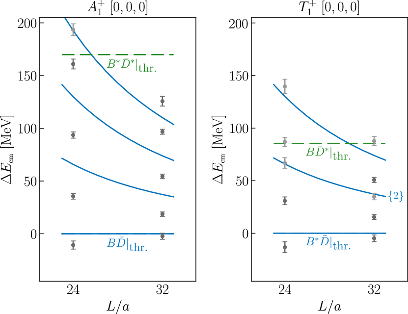
Figure 1: Left: The finite-volume energies of the $\bar{b}\bar{c}ud$ system with $I(J^{P})=0(0^{+})$ as a function of the spatial lattice size. The data points with error bars show the actual finite-volume energy levels; points plotted with a lighter shade of gray are excluded from the Lüscher analysis. The solid blue curves correspond to what would be the noninteracting $B$-$\bar{D}$ energy levels, the lowest of which coincides with the strong-decay threshold. The dashed green line shows the $B^{*}$-$\bar{D}^{*}$ threshold. Right: The corresponding plot for $I(J^{P})=0(1^{+})$. Here, the solid blue curves correspond to what would be the noninteracting $B^{*}$-$\bar{D}$ energy levels, and the dashed green line corresponds to the $B$-$\bar{D}^{*}$ threshold. In this case, the second noninteracting energy level (as well as higher levels not shown) is degenerate since both $S$ and $D$ waves contribute to the quantum numbers $J^{P}=1^{+}$ for pseudoscalar-vector scattering; the label $\{2\}$ shows the multiplicity.

Our results for the lowest five energy levels of each $\bar{b}\bar{c}ud$ system are shown as a function of the spatial lattice size $N_{s}=L/a$ in Fig. 1. Also shown are the lowest four noninteracting $B^{(*)}$-$\bar{D}$ energy levels, calculated as $E=E_{B^{(*)}}(\mathbf{p}^{2})+E_{\bar{D}}(\mathbf{p}^{2})$ with momenta $\mathbf{p}$ satisfying the periodic boundary conditions [each component an integer multiple of $2\pi/L$], and with the single-meson energies calculated on the lattice and described by the dispersion relations

$$E_{B^{(*)}}(\mathbf{p}^{2})= E_{B^{(*)}}(0)+\sqrt{m_{B^{(*)},{\rm kin}}^{2}+\mathbf{p}^{2}}-m_{B^{(*)},{\rm kin}},$$

$$E_{D}(\mathbf{p}^{2})= E_{\bar{D}}(0)+\mathbf{p}^{2}/(2m_{\bar{D},{\rm kin}})-\mathbf{p}^{4}/(8m_{\bar{D},4}^{3}).$$ (2)

The values of $E_{B^{(*)}}(0)$,  $m_{B^{(*)},{\rm kin}}$,  $E_{\bar{D}}(0)$,  $m_{\bar{D},{\rm kin}}$, and $m_{\bar{D},4}$ are provided in the supplemental material. In Fig. 1 we see that the actual $\bar{b}\bar{c}ud$ energy levels are shifted significantly relative to the noninteracting levels due to the meson-meson interactions in the finite volume, except for the third level in the case of $J=1$ (we discuss the reason for this behavior farther below). Moreover, for both $J=0$ and $J=1$, the number of observed levels in the energy range considered here is larger than in the noninteracting case by one, which is a first hint for the existence of a pole in the scattering amplitude. The observed ground-state energies are only a few MeV below threshold, but the first excited-state energies are far below the $|\mathbf{p}|=2\pi/L$ noninteracting two-meson levels and will ultimately be identified as the $|\mathbf{p}|=0$ levels for large $L$ if there are shallow bound states.

To rigorously investigate whether bound states or resonances exist, we map the observed finite-volume energy levels $E_{n}$ to infinite-volume $S$-wave $B^{(*)}$-$\bar{D}$ scattering phase shifts $\delta_{0}(k_{n})$ using the Lüscher quantization condition

$$\cot{\delta_{0}(k_{n})}=\frac{2Z_{00}(1;(k_{n}L/2\pi)^{2})}{\pi^{1/2}k_{n}L},$$ (3)

where $Z_{00}$ is the generalized zeta function [23] and $k_{n}$ is the scattering momentum associated with energy level $E_{n}$, calculated from $E_{n}=E_{B^{(*)}}(k_{n}^{2})+E_{\bar{D}}(k_{n}^{2})$ with the dispersion relations (2). To ensure that the single-channel, single-partial-wave approximation is applicable, we only extract the phase shifts for the energy levels below the $B^{*}$-$\bar{D}^{*}$ ($J=0$) and $B$-$\bar{D}^{*}$ ($J=1$) thresholds. Furthermore, for $J=1$, we observe that the third finite-volume energy level is consistent with the noninteracting $|\mathbf{p}|=2\pi/L$ energy level that has multiplicity 2 once including both $S$-wave and $D$-wave structures, as we did in our operator basis. Because finite-volume interactions for higher partial waves are suppressed, we conclude that this energy level is dominantly $D$-wave, and we therefore exclude it from the Lüscher analysis. This is further corroborated by the eigenvectors from the GEVP, which show that this state has a non-negligible overlap only with the operator $\mathcal{O}^{T_{1}^{+}}_{7}$ that was subduced from a $D$-wave structure.

		$\Delta m_{\rm BS}$ [MeV]		$\Delta m_{\textrm{R}}$ [MeV]		$\Gamma_{\textrm{R}}$ [MeV]
$J\!=\!0$		$-0.5(0.9)$		$138(13)$		$229(35)$
$J\!=\!1$		$-2.4(2.9)$		$\phantom{0}67(24)$		$132(32)$

Table 2: Our results for the $\bar{b}\bar{c}ud$ bound-state (BS) and resonance (R) pole locations, where $\Delta m_{\rm BS}=m_{\rm BS}-m_{B^{(*)}}-m_{\bar{D}}$, $\Delta m_{\textrm{R}}=\mathrm{Re}(\sqrt{s_{\textrm{R}}})-m_{B^{(*)}}-m_{\bar{D}}$, and $\Gamma_{\textrm{R}}=-2\>\mathrm{Im}(\sqrt{s_{\textrm{R}}})$. Only the statistical uncertainties are given.

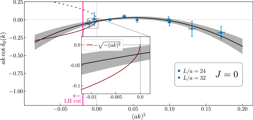
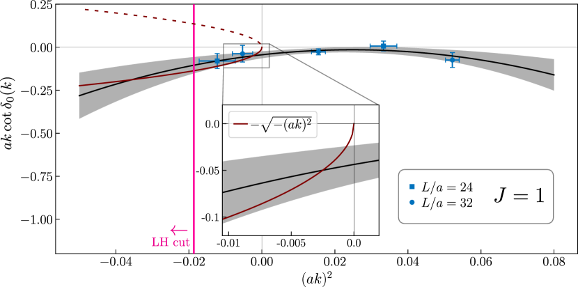
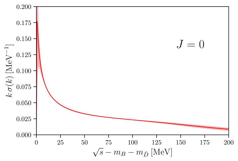
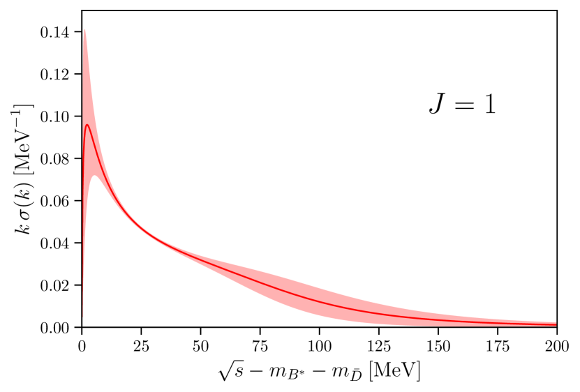
Figure 2: Left: Our results for the functions $ak\cot\delta_{0}(k)$ for $S$-wave $B$-$\bar{D}$ scattering (top) and $S$-wave $B^{*}$-$\bar{D}$ scattering (bottom), where $k$ is the scattering momentum, $\delta_{0}(k)$ is the scattering phase shift, and $a=0.11887(80)$ fm is the lattice spacing. The data points were obtained directly from the lattice energy levels, and the curves correspond to ERE fits through order $k^{4}$. Also shown are the functions $-\sqrt{-(ak)^{2}}$ (solid red parabolas) whose intersections with $ak\cot\delta_{0}(k)$ just below threshold correspond to the shallow $\bar{b}\bar{c}ud$ bound states we predict, and $+\sqrt{-(ak)^{2}}$ (dashed red parabolas) whose intersections with $ak\cot\delta_{0}(k)$ would correspond to virtual $\bar{b}\bar{c}ud$ bound states. The vertical magenta lines show the positions of two-pion-exchange left-hand branch points. Right: Our results for the product of scattering momentum and $B^{(*)}$-$\bar{D}$ scattering cross section, which is proportional to the scattering rate, as a function of center-of-momentum energy.

Our results for the scattering phase shifts, along with effective-range expansion (ERE) fits of the form

$$k\cot\delta_{0}(k)=\frac{1}{a_{0}}+\frac{1}{2}r_{0}k^{2}+b_{0}k^{4},$$ (4)

are shown in Fig. 2 (Left). The numerical values of the fitted ERE parameters are given in the supplemental material. The scattering phase shift is related to the $S$-wave scattering amplitude and cross section by

$$T_{0}(k)=\frac{1}{\cot\delta_{0}(k)-i},\hskip 17.22217pt\sigma(k)=\frac{4\pi}{k^{2}}|T_{0}(k)|^{2}.$$ (5)

Poles of $T_{0}(k)$ at purely imaginary $k$ correspond to genuine or virtual bound states for $\mathrm{Im}(k)>0$ or $\mathrm{Im}(k)<0$, respectively, while poles with $\mathrm{Re}(k)\neq 0$ and $\mathrm{Im}(k)<0$ correspond to resonances. Using our ERE fits, we find genuine bound-state poles as well as resonance poles for both $J=0$ and $J=1$ at the values of $\sqrt{s}-\sqrt{s_{\rm th}}=\sqrt{m_{B^{(\ast)}}^{2}+k^{2}}+\sqrt{m_{\bar{D}}^{2}+k^{2}}-m_{B^{(*)}}-m_{\bar{D}}$ given in Table 2 ($s$ denotes the Mandelstam variable equal to the square of the center-of-momentum energy). We used our lattice results for the kinetic $B^{(*)}$ and $\bar{D}$ masses to evaluate this expression; to obtain predictions for absolute tetraquark bound state or resonance masses, one simply needs to add the experimental value of the threshold energy, $m_{B^{(*)}}^{\text{exp}}+m_{\bar{D}}^{\text{exp}}$.

The resonances have masses of order $100$ MeV above the $B^{(*)}$-$\bar{D}$ thresholds and decay widths of order $200$ MeV. We caution that the resonance poles lie outside the radius of convergence of the ERE, which is limited by the presence of a left-hand cut associated with two-pion $t$-channel exchange in the scattering process (single-pion exchange would require a $D^{*}$ in the initial or final state, and is therefore not relevant here). The center-of-momentum energy at which the left-hand cut starts is obtained from the kinematic relations for the Mandelstam variables by expressing $s$ in terms of $t$ and the scattering angle $\theta^{*}$, and then setting $t=(2m_{\pi})^{2}$ and $\theta^{*}=\pi$ [54]; this gives $\sqrt{s_{\rm cut}}-\sqrt{s_{\rm th}}\approx-18\>{\rm MeV}$ for both $J=0$ and $J=1$, corresponding to $(ak)^{2}_{\rm cut}\approx-0.019$, as indicated with the magenta lines in Fig. 2. While our ERE fit is seen to describe the data very well for real $(ak)^{2}$ in the full momentum range, the prediction of resonance poles away from the real axis may be less reliable. To test the stability, we also performed ERE fits through order $k^{6}$. The coefficients of $k^{6}$ are found to be consistent with zero within the statistical uncertainties, and the other parameters remain consistent with those from the order-$k^{4}$ fit. For $J=0$, the resonance pole obtained from the order-$k^{6}$ fit is at a similar location. For $J=1$, where we have fewer data points, the uncertainties from the $k^{6}$ fit are too large to determine the pole locations.

The bound-state poles are extremely close to threshold and therefore well within the region of validity of the ERE. However, their nature could change through statistical fluctuations, as can be seen from the $\pm\sqrt{-(ak)^{2}}$ parabolas in Fig. 2 (Left). For both $J=0$ and $J=1$, an upward fluctuation of our $k\cot\delta_{0}(k)$ curve would turn the genuine bound state into a virtual bound state, which is not an asymptotic state in QCD but would still strongly affect the $B^{(*)}$-$\bar{D}$ scattering rates near threshold [55]. For $J=0$, a downward fluctuation by $\lesssim 3\sigma$ would still preserve the genuine bound state, while for $J=1$ already a $\sim 1\sigma$ downward fluctuation would lead to the disappearance of the pole. To further test our prediction of shallow bound states, we performed additional ERE fits of order $k^{0}$ and order $k^{2}$ using only the three data points closest to threshold, which are within the strict radius of convergence of the ERE. These fits give consistent results for the bound-state masses, and the order-$k^{0}$ fits yield even higher statistical significance for the existence of the (genuine or virtual) shallow bound states. The details of these fits are shown in the supplemental material.

Returning to the discussion of our main fits as shown in Fig. 2, we note that, in addition to the shallow-bound-state and the broad-resonance poles, we find poles with purely imaginary $k$ far below threshold (and on the left-hand cut) that violate the bound-state consistency condition discussed in Ref. [56] and therefore do not correspond to physical states (bound states this far below threshold are also ruled out by the absence of corresponding finite-volume energy levels).

The scattering rate (probability per time) is equal to the product of flux and cross section, and hence proportional to $k\,\sigma(k)$ for nonrelativistic $k$. These products are shown in Fig. 2 (Right) as a function of the center-of-momentum energy. We emphasize that the scattering rates only depend on our fit functions for real-valued $k^{2}$ that interpolate our data very well, so these predictions are also expected to be very reliable. We observe sharp enhancements in the scattering rates close to the thresholds, related to the shallow bound states or virtual bound states. At higher energies, the scattering rates continue to be enhanced, likely by the broad resonances. The scattering rates are very close to the largest possible value allowed by unitarity, given by $|T_{0}|^{2}=1$, up to several tens of MeV above threshold.

In summary, the substantial improvements made here in determining the $\bar{b}\bar{c}ud$ finite-volume energy levels allowed us to determine the detailed energy dependence of the $B$-$\bar{D}$ and $B^{*}$-$\bar{D}$ $S$-wave scattering amplitudes for the first time using lattice QCD, revealing very interesting strong-interaction phenomena. We found poles for both $J=0$ and $J=1$ corresponding to shallow bound states, as well as hints for poles corresponding to broad resonances. While further lattice-QCD computations at additional lattice spacings and pion masses will be needed to pin down the exact location and nature of each pole at the physical point, we expect our prediction of shallow bound states, either genuine or virtual, to be quite robust. The possible resonances above threshold are very broad and are therefore presumably difficult to observe at the LHC and future experiments. On the other hand, if the $J=0$ pole just below the $B$-$\bar{D}$ threshold is confirmed as a genuine bound state, this isoscalar, scalar $\bar{b}\bar{c}ud$ tetraquark will decay through the weak interaction only and could become the first tetraquark to be observed at the LHC with this feature. If the $J=1$ pole just below the $B^{*}$-$\bar{D}$ threshold is confirmed as a genuine bound state, it will decay electromagnetically into $B\bar{D}\gamma$ (and also into the $J=0$ tetraquark plus a photon, if that tetraquark is confirmed as a genuine bound state).

Supplemental material

I Operators

For the $\bar{b}\bar{c}ud$ system with $I(J^{P})=0(0^{+})$, we use the seven operators

$$\mathcal{O}_{1}^{A_{1}^{+}}= \frac{1}{\sqrt{V_{S}}}\sum_{\mathbf{x}}\bar{b}(\mathbf{x})\gamma_{5}u(\mathbf{x})\,\bar{c}(\mathbf{x})\gamma_{5}d(\mathbf{x})-(d\leftrightarrow u),$$ (6)

$$\mathcal{O}_{2}^{A_{1}^{+}}= \frac{1}{\sqrt{V_{S}}}\sum_{\mathbf{x}}\bar{b}(\mathbf{x})\gamma_{j}u(\mathbf{x})\,\bar{c}(\mathbf{x})\gamma_{j}d(\mathbf{x})-(d\leftrightarrow u),$$ (7)

$$\mathcal{O}_{3}^{A_{1}^{+}}= \frac{1}{\sqrt{V_{S}}}\sum_{\mathbf{x}}\bar{b}^{a}(\mathbf{x})\gamma_{5}C\bar{c}^{b,T}(\mathbf{x})\,u^{a,T}(\mathbf{x})C\gamma_{5}d^{b}(\mathbf{x})-(d\leftrightarrow u),$$ (8)

$$\mathcal{O}^{A_{1}^{+}}_{4}= \;B^{+}(\mathbf{0})\,D^{-}(\mathbf{0})-(d\leftrightarrow u),\vphantom{\sum_{x}}$$ (9)

$$\mathcal{O}^{A_{1}^{+}}_{5}= \sum_{\mathbf{q}=\pm\mathbf{e}_{i=x,y,z}}B^{+}(\mathbf{q})\,D^{-}(-\mathbf{q})-(d\leftrightarrow u),$$ (10)

$$\mathcal{O}^{A_{1}^{+}}_{6}= \sum_{\mathbf{q}=\pm\mathbf{e}_{i}\pm\mathbf{e}_{j},\,i<j}B^{+}(\mathbf{q})\,D^{-}(-\mathbf{q})-(d\leftrightarrow u),$$ (11)

$$\mathcal{O}^{A_{1}^{+}}_{7}= \sum_{\mathbf{q}=\pm\mathbf{e}_{x}\pm\mathbf{e}_{y}\pm\mathbf{e}_{z}}B^{+}(\mathbf{q})\,D^{-}(-\mathbf{q})-(d\leftrightarrow u),$$ (12)

where the repeated index $j$ is summed over the spatial directions, the repeated color indices $a$ and $b$ are summed over the three colors, $V_{S}=L^{3}$ is the spatial lattice volume, and

$$B^{+}(\mathbf{q})= \frac{1}{\sqrt{V_{S}}}\sum_{\mathbf{x}}\,\bar{b}(\mathbf{x})\gamma_{5}u(\mathbf{x})\,e^{i\frac{2\pi}{L}\mathbf{q}\cdot\mathbf{x}},$$ (13)

$$D^{-}(\mathbf{q})= \frac{1}{\sqrt{V_{S}}}\sum_{\mathbf{x}}\,\bar{c}(\mathbf{x})\gamma_{5}d(\mathbf{x})\,e^{i\frac{2\pi}{L}\mathbf{q}\cdot\mathbf{x}}.$$ (14)

The operators $\mathcal{O}_{1}^{A_{1}^{+}}$ and $\mathcal{O}_{2}^{A_{1}^{+}}$ are constructed as products of color-singlet $B$, $\bar{D}$ and $B^{*}$, $\bar{D}^{*}$ operators at the same spacetime point that are then jointly projected to zero momentum by summing over the spatial coordinates. The operator $\mathcal{O}_{3}^{A_{1}^{+}}$ is constructed as a color-singlet contraction of two color-nonsinglet diquarks at the same spacetime point that is then jointly projected to zero momentum. The operators $\mathcal{O}_{4}^{A_{1}^{+}}$ through $\mathcal{O}_{7}^{A_{1}^{+}}$ are $B$-$\bar{D}$ “scattering” operators in which the $B$ and $\bar{D}$ operators are individually momentum-projected and have back-to-back momenta of magnitudes $0$, $2\pi/L$, $\sqrt{2}\cdot 2\pi/L$, and $\sqrt{3}\cdot 2\pi/L$ ($L$ is the spatial lattice size). For the scattering operators, the summations over the back-to-back momentum directions ensure that the operators transform in the $A_{1}^{+}$ irrep of the octahedral group that contains $J=0$.

All quark fields in the above expressions are smeared using gauge-covariant Gaussian smearing (see e.g. Eq. (8) in Ref. [11]), with $(\sigma_{\text{Gauss}},N_{\textrm{Gauss}})=(4.47,35),(1.195,5),(1.0,10)$ for the light, charm, and bottom quarks, respectively. The gauge links used for the Gaussian smearing are APE smeared (see e.g. Eq. (23) in Ref. [57]) with parameters $N_{\textrm{APE}}=50$ and $\alpha_{\textrm{APE}}=0.5$. The smearing parameters are identical at source and sink, leading to symmetric correlation matrices.

For the $\bar{b}\bar{c}ud$ system with $I(J^{P})=0(1^{+})$, we use the eight operators

$$\mathcal{O}_{1,k}^{T_{1}^{+}}= \frac{1}{\sqrt{V_{S}}}\,\sum_{\mathbf{x}}\bar{b}(\mathbf{x})\gamma_{k}u(\mathbf{x})\,\bar{c}(\mathbf{x})\gamma_{5}d(\mathbf{x})-(d\leftrightarrow u),$$ (15)

$$\mathcal{O}_{2,k}^{T_{1}^{+}}= \frac{1}{\sqrt{V_{S}}}\,\sum_{\mathbf{x}}\bar{b}(\mathbf{x})\gamma_{5}u(\mathbf{x})\,\bar{c}(\mathbf{x})\gamma_{k}d(\mathbf{x})-(d\leftrightarrow u),$$ (16)

$$\mathcal{O}_{3,k}^{T_{1}^{+}}= \frac{1}{\sqrt{V_{S}}}\,\,\epsilon_{kjl}\sum_{\mathbf{x}}\bar{b}(\mathbf{x})\gamma_{j}u(\mathbf{x})\,\bar{c}(\mathbf{x})\gamma_{l}d(\mathbf{x})-(d\leftrightarrow u),$$ (17)

$$\mathcal{O}_{4,k}^{T_{1}^{+}}= \frac{1}{\sqrt{V_{S}}}\,\sum_{\mathbf{x}}\bar{b}^{a}(\mathbf{x})\gamma_{k}C\bar{c}^{b,T}(\mathbf{x})\,u^{a,T}(\mathbf{x})C\gamma_{5}d^{b}(\mathbf{x})-(d\leftrightarrow u),$$ (18)

$$\mathcal{O}^{T_{1}^{+}}_{5,k}= \;B_{k}^{*+}(\mathbf{0})\,D^{-}(\mathbf{0})-(d\leftrightarrow u),\vphantom{\sum_{x}}$$ (19)

$$\mathcal{O}^{T_{1}^{+}}_{6,k}= \sum_{\mathbf{q}=\pm\mathbf{e}_{i=x,y,z}}B_{k}^{*+}(\mathbf{q})\,D^{-}(-\mathbf{q})-(d\leftrightarrow u),$$ (20)

$$\mathcal{O}^{T_{1}^{+}}_{7,z}= \sum_{\mathbf{q}=\pm\mathbf{e}_{i=x,y}}B_{z}^{*+}(\mathbf{q})\,D^{-}(-\mathbf{q})-2\sum_{\mathbf{q}^{\prime}=\pm\mathbf{e}_{z}}B_{z}^{*+}(\mathbf{q}^{\prime})\,D^{-}(-\mathbf{q}^{\prime})-(d\leftrightarrow u),$$ (21)

$$\mathcal{O}^{T_{1}^{+}}_{8,k}= \sum_{\mathbf{\mathbf{q}}=\pm\mathbf{e}_{i}\pm\mathbf{e}_{j},i<j}B_{k}^{*+}(\mathbf{q})\,D^{-}(-\mathbf{q})-(d\leftrightarrow u),$$ (22)

where $D^{-}(\mathbf{q})$ was defined in Eq. (14),

$$B_{k}^{*+}(\mathbf{q})=\frac{1}{\sqrt{V_{S}}}\sum_{\mathbf{x}}\,\bar{b}(\mathbf{x})\gamma_{k}u(\mathbf{x})\,e^{i\frac{2\pi}{L}\mathbf{q}\cdot{\mathbf{x}}},$$ (23)

and $k=x,y,z$ denotes the spatial polarization direction (the operator $\mathcal{O}^{T_{1}^{+}}_{7}$ is shown for $k=z$ only). These operators transform in the $T_{1}^{+}$ irrep of the octahedral group that contains $J=1$. The operators $\mathcal{O}_{1}^{T_{1}^{+}}$, $\mathcal{O}_{2}^{T_{1}^{+}}$, and $\mathcal{O}_{3}^{T_{1}^{+}}$ are constructed as products of color-singlet $B^{(*)}$ and $\bar{D}^{(*)}$ operators at the same spacetime point that are then jointly projected to zero momentum by summing over the spatial coordinates. The operator $\mathcal{O}_{4}^{T_{1}^{+}}$ is constructed as a color-singlet contraction of two color-nonsinglet diquarks at the same spacetime point that is then jointly projected to zero momentum. Here, the two heavy quarks are combined to a flavor-symmetric spin-1 diquark and the two light quarks are combined to a flavor-antisymmetric spin-0 diquark. The operators $\mathcal{O}_{5}^{T_{1}^{+}}$ through $\mathcal{O}_{8}^{T_{1}^{+}}$ are $B^{*}$-$\bar{D}$ scattering operators in which the $B^{*}$ and $\bar{D}$ have back-to-back momenta of magnitudes $0$, $2\pi/L$ (for both $\mathcal{O}_{6}^{T_{1}^{+}}$ and $\mathcal{O}_{7}^{T_{1}^{+}}$), and $\sqrt{2}\cdot 2\pi/L$. Two different operators are used for the case with one unit of back-to-back momentum to account for the mixing of $S$ and $D$ partial waves [47]. Again, all quark fields are smeared, with the same parameters as used for $J=0$.

II $\bm{\bar{D}^{(*)}}$ and $\bm{B^{(*)}}$ dispersion relations

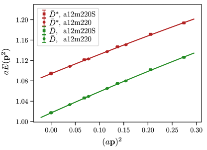
Figure 3: Results for $aE_{\bar{D}}(\mathbf{p}^{2})$ and $aE_{\bar{D}^{*}}(\mathbf{p}^{2})$ for $0\leq\mathbf{p}^{2}\leq 4(2\pi/L)^{2}$ from the two ensembles, along with fits of the form (24).

Our results for the $\bar{D}$ and $\bar{D}^{*}$ meson energies as a function of spatial momentum squared are shown in Fig. 3. We performed fits to the combined data from the two ensembles using the three-parameter form

$$E_{\bar{D}^{(*)}}(\mathbf{p}^{2})=E_{\bar{D}^{(*)}}(0)+\frac{\mathbf{p}^{2}}{2m_{\bar{D}^{(*)},{\rm kin}}}-\frac{\mathbf{p}^{4}}{8m_{\bar{D}^{(*)},4}^{3}}$$ (24)

to allow for different values of $m_{\bar{D}^{(*)},{\rm kin}}$, and $m_{\bar{D}^{(*)},4}$ due to discretization errors. Higher powers of $\mathbf{p}$ are expected to be negligible for the momentum range we use. The fit results are given in Table 3. The spin-averaged kinetic mass agrees with the experimental value [50] within $3\%$, confirming the successful tuning of the charm-quark mass according to the Fermilab method [49]. We also find that the results for $m_{\bar{D}^{(*)},4}$ are actually consistent with $m_{\bar{D}^{(*)},{\rm kin}}$ within the statistical uncertainties.

$aE_{\bar{D}}(0)$	$aE_{\bar{D}^{*}}(0)$	$am_{\bar{D},\textrm{kin}}$	$am_{\bar{D}^{*},\textrm{kin}}$	$am_{\bar{D},4}$	$am_{\bar{D}^{*},4}$
$1.01718(38)$	$1.09434(60)$	$1.172(14)$	$1.294(25)$	$1.09(9)$	$1.18(16)$

Table 3: $\bar{D}$ and $\bar{D}^{*}$ meson dispersion-relation parameters in lattice units, obtained from combined fits to the data from the a12m220S and a12m220 ensembles.

For the $B$ and $B^{*}$ mesons, we did not expect a significant difference between $m_{B^{(*)},{\rm kin}}$, and $m_{B^{(*)},4}$ due to the high level of improvement of the lattice NRQCD action [51], and we therefore performed two-parameter fits of the form

$$E_{B^{(*)}}(\mathbf{p}^{2})=E_{B^{(*)}}(0)+\sqrt{m_{B^{(*)},{\rm kin}}^{2}+\mathbf{p}^{2}}-m_{B^{(*)},{\rm kin}}.$$ (25)

$aE_{B}(0)$	$aE_{B^{*}}(0)$	$am_{B,\textrm{kin}}$	$am_{B^{*},\textrm{kin}}$
$0.4823(12)$	$0.5077(13)$	$3.121(84)$	$3.091(89)$

Table 4: $B$ and $B^{*}$ meson dispersion-relation parameters in lattice units, obtained from combined fits to the data from the a12m220S, a12m220, and a12m220L ensembles [58].

These fits included also a third ensemble of gauge configurations, a12m220L, with the same bare parameters and an even larger volume, and are discussed in more detail in Ref. [58]. The data from all three ensembles are well-described jointly by Eq. (25) with the parameters given in Table 4. The spin-averaged kinetic $B$-meson mass is within 4% of the experimental value [50].

III $\bm{\bar{b}\bar{c}ud}$ energies and $\bm{B^{(*)}}$-$\bm{\bar{D}}$ scattering phase shifts

Plots of the effective energies of the five lowest eigenvalues obtained from the GEVP for the $\bar{b}\bar{c}ud$ correlation matrices are shown in Fig. 4. We determine the energy levels $E_{n}$ by carrying out correlated least-$\chi^{2}$ fits of the form $\lambda_{n}(t,t_{0})=A_{n}e^{-E_{n}t}$. We perform fits for multiple different ranges $t_{\text{min}}\leq t\leq t_{\text{max}}$ with sufficiently large $t_{\text{min}}$ to ensure single-exponential behavior and obtain the final estimate for $E_{n}$ from a weighted average that takes into account correlations and lowers the weights of fits with $\chi^{2}/{\rm d.o.f.}>1$, following the FLAG averaging procedure [53] (see also our discussion in Appendix B of Ref. [13]). The statistical uncertainties are calculated and propagated to the further analysis using jackknife.

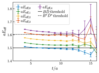
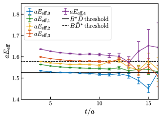
Figure 4: Left: Effective energies $aE_{{\rm eff},n}(t)=\ln(\lambda_{n}(t,t_{0})/\lambda_{n}(t+a,t_{0}))$ of the five lowest eigenvalues $\lambda_{0}(t,t_{0}),...,\lambda_{4}(t,t_{0})$ of the $\bar{b}\bar{c}ud$ system with $I(J^{P})=0(0^{+})$ on the a12m220S lattice, obtained by solving the GEVP for the $7\times 7$ correlation matrix. For sufficiently large $t$, these effective energies correspond to the five lowest finite-volume energy levels with the given quantum numbers. Also shown are the strong-decay-threshold energies computed on the same lattice. Note that all absolute energies contain an overall constant shift due to the use of NRQCD and of the Fermilab method. Right: The corresponding plot for the $\bar{b}\bar{c}ud$ system with $I(J^{P})=0(1^{+})$, using the $8\times 8$ correlation matrix.

Our results for the $\bar{b}\bar{c}ud$ finite-volume energies, their values relative to the threshold, the corresponding scattering momenta squared, and the corresponding products of scattering momentum and cotangent of $S$-wave scattering phase shifts are listed in Tables 5 (for the $A_{1}^{+}$ irrep relevant for $J^{P}=0^{+}$) and 6 (for the $T_{1}^{+}$ irrep relevant for $J^{P}=1^{+}$). As discussed in the main article, some high-lying energy levels are excluded from the phase-shift determination because they lie above inelastic thresholds, and the third energy level in the $T_{1}^{+}$ irrep is excluded because it corresponds to a state dominated by a $D$ wave; these cases are labeled “N/A” in the tables.

Ensemble	$aE$	$a\Delta E$	$(ak)^{2}$	$ak\cot\delta_{0}$
a12m220S	$1.4937(27)$	$-0.0065(23)$	$-0.0100(35)$	$-0.057(42)$
	$1.5217(16)$	$\phantom{-}0.0215(17)$	$\phantom{-}0.0378(24)$	$\phantom{-}0.046(23)$
	$1.5568(17)$	$\phantom{-}0.0566(18)$	$\phantom{-}0.0987(26)$	$-0.001(42)$
	$1.5975(25)$	$\phantom{-}0.0973(28)$	$\phantom{-}0.1706(46)$	$-0.181(87)$
	$1.6172(36)$	$\phantom{-}0.1170(34)$	N/A	N/A
a12m220	$1.4975(17)$	$-0.0014(17)$	$-0.0035(25)$	$\phantom{-}0.008(90)$
	$1.5102(11)$	$\phantom{-}0.0112(13)$	$\phantom{-}0.0182(17)$	$-0.001(17)$
	$1.5318(11)$	$\phantom{-}0.0329(13)$	$\phantom{-}0.0554(17)$	$-0.004(35)$
	$1.5574(12)$	$\phantom{-}0.0585(14)$	$\phantom{-}0.0999(19)$	$-0.037(48)$
	$1.5750(29)$	$\phantom{-}0.0760(28)$	$\phantom{-}0.1307(43)$	$-0.13(11)\phantom{0}$

Table 5: The $\bar{b}\bar{c}ud$ finite-volume energies in the $A_{1}^{+}$ irrep, their values relative to the $B$-$\bar{D}$ threshold, the corresponding $B$-$\bar{D}$ scattering momenta squared, and the corresponding products of scattering momentum and cotangent of scattering phase shift (all in lattice units). Note that the absolute energies contain an overall constant offset due to the use of NRQCD and of the Fermilab method; this offset cancels in the differences to the threshold.

Ensemble	$aE$	$a\Delta E$	$(ak)^{2}$	$ak\cot\delta_{0}$
a12m220S	$1.5176(40)$	$-0.0080(31)$	$-0.0122(49)$	$-0.080(44)$
	$1.5443(24)$	$\phantom{-}0.0187(22)$	$\phantom{-}0.0333(37)$	$\phantom{-}0.007(29)$
	$1.5661(46)$	$\phantom{-}0.0404(31)$	N/A	N/A
	$1.5783(30)$	$\phantom{-}0.0526(26)$	N/A	N/A
	$1.6101(45)$	$\phantom{-}0.0844(41)$	N/A	N/A
a12m220	$1.5217(19)$	$-0.0029(19)$	$-0.0053(28)$	$-0.037(48)$
	$1.5339(13)$	$\phantom{-}0.0093(14)$	$\phantom{-}0.0155(19)$	$-0.027(18)$
	$1.5456(16)$	$\phantom{-}0.0210(18)$	N/A	N/A
	$1.5553(13)$	$\phantom{-}0.0307(15)$	$\phantom{-}0.0522(19)$	$-0.074(43)$
	$1.5776(27)$	$\phantom{-}0.0530(26)$	N/A	N/A

Table 6: The $\bar{b}\bar{c}ud$ finite-volume energies in the $T_{1}^{+}$ irrep, their values relative to the $B^{*}$-$\bar{D}$ threshold, the corresponding $B^{*}$-$\bar{D}$ scattering momenta squared, and the corresponding products of scattering momentum and cotangent of scattering phase shift (all in lattice units). Note that the absolute energies contain an overall constant offset due to the use of NRQCD and of the Fermilab method; this offset cancels in the differences to the threshold.

IV ERE fit parameters using the full momentum range

This section contains our results for the ERE fit parameters for the main fits that use all available scattering momenta and phase shifts from Tables 5 and 6. The fits were performed in lattice units,

$$ak\cot\delta_{0}=\frac{a}{a_{0}}+\frac{r_{0}}{2a}(ak)^{2}+\frac{b_{0}}{a^{3}}(ak)^{4},$$ (26)

where $a$ is the lattice spacing. We used the coefficients of $(ak)^{0}$, $(ak)^{2}$, and $(ak)^{4}$ as the fit parameters. Our results for these parameters, along with their correlation matrices, are given in Tables 7 and 8. In addition, we provide the values of $1/a_{0}$, $r_{0}$, and $b_{0}$ in physical units in Table 9.

Parameter	Value	Correlation Matrix
$a/a_{0}$	$-0.022(18)$	$1$	$-0.715$	$\phantom{-}0.621$
$r_{0}/(2a)$	$\phantom{-}1.92(69)$	$-0.715$	$1$	$-0.889$
$b_{0}/a^{3}$	$-18.4(5.0)$	$\phantom{-}0.621$	$-0.889$	$1$

Table 7: Fit results for the $J=0$ ERE parameters and their correlation matrix.

Parameter	Value	Correlation Matrix
$a/a_{0}$	$-0.044(20)$	$1$	$-0.725$	$\phantom{-}0.594$
$r_{0}/(2a)$	$\phantom{-}2.4(1.3)$	$-0.725$	$1$	$-0.869$
$b_{0}/a^{3}$	$-48(24)$	$\phantom{-}0.594$	$-0.869$	$1$

Table 8: Fit results for the $J=1$ ERE parameters and their correlation matrix.

	$1/a_{0}$ [fm-1]	$r_{0}$ [fm]	$b_{0}$ [fm3]
$J\!=\!0$	$-0.19(16)$	$0.46(16)$	$-0.031(8)\phantom{0}$
$J\!=\!1$	$-0.37(17)$	$0.56(30)$	$-0.080(41)$

Table 9: The ERE parameters in physical units.

V ERE fits and bound-state poles using only the low-momentum region

Our ERE fits to only the three data points closest to the thresholds are shown in Fig. 5. In this momentum region, 0th-order fits already describe the data well; for comparison, we also show fits through order $k^{2}$. The resulting ERE parameters and bound-state pole masses are given in Tables 10 and 11.

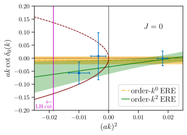
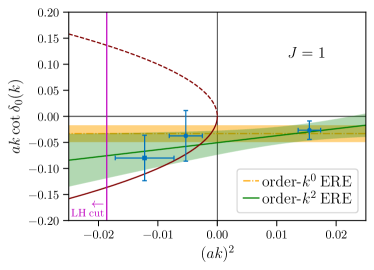
Figure 5: ERE fits using only the three data points closest to the thresholds for $S$-wave $B$-$\bar{D}$ scattering (left) and $S$-wave $B^{*}$-$\bar{D}$ scattering (right); here, $a$ is the lattice spacing. Also shown are the functions $-\sqrt{-(ak)^{2}}$ (solid red parabolas) whose intersections with $ak\cot\delta_{0}(k)$ just below threshold correspond to the shallow $\bar{b}\bar{c}ud$ bound states we predict, and $+\sqrt{-(ak)^{2}}$ (dashed red parabolas) whose intersections with $ak\cot\delta_{0}(k)$ would correspond to virtual $\bar{b}\bar{c}ud$ bound states. The vertical magenta lines show the positions of two-pion-exchange left-hand branch points.

	$1/a_{0}$ [fm-1]	$\Delta m_{\rm BS}$ [MeV]
$J\!=\!0$	$-0.07(13)$	$-0.07(25)$
$J\!=\!1$	$-0.28(14)$	$-1.0(1.0)$

Table 10: Results for the inverse scattering lengths and bound-state masses (relative to the $B^{(*)}$-$\bar{D}$ thresholds) from the order-$k^{0}$ ERE fits to the three data points closest to the threshold.

	$1/a_{0}$ [fm-1]	$r_{0}$ [fm]	$\Delta m_{\rm BS}$ [MeV]
$J\!=\!0$	$-0.28(23)$	$0.37(34)$	$-1.2(2.2)$
$J\!=\!1$	$-0.43(14)$	$0.32(30)$	$-2.9(3.2)$

Table 11: Results for the ERE parameters and bound-state masses (relative to the $B^{(*)}$-$\bar{D}$ thresholds) from the order-$k^{2}$ ERE fits to the three data points closest to the threshold.