Integration with respect to the Lefschetz number
Abstract.
We develop a theory of integration with respect to the Lefschetz number in the context of o-minimal structures containing the semilinear sets. We prove several results and we apply the theory to the field of object detention using sensors.
1. Introduction
The Lefschetz number of a continuous map between compact polyhedra is a classical topological invariant defined as
| (1) |
where denotes the induced morphism in homology with rational coefficients (see [1]). The Lefschetz number is an invariant of great importance in Algebraic Topology. In addition to being a generalization of the Euler-Poincaré characteristic, which is recovered by considering to be the identity, the Lefschetz number provides a bridge between Topology and Dynamics by means of guaranteeing certain fixed point theorems.
The goal of this paper is to develop a theory of integration with respect to the Lefschetz number, considered as a measure (more formally: a lattice valuation). The idea of integration with respect to topological invariants dates back, at least, to the work of Blaschke in Geometry [3], where integration with respect to the Euler-Poincaré charactersitic performed its appearance. Integration with respect to the Euler-Poincaré characteristic, also referred as Euler Calculus, was approached since then from many perspectives and within many fields of Mathematics, ranging from Algebraic Geometry ([8]) and Sheaf Theory ([12]) to Analysis ([6]). In more recent times, Euler Calculus has become a resourceful tool for applications ([5]).
In order construct a theory of integration with respect to the Lefschetz number, firstly we need and algebra of sets. However, the subcomplexes of a simplicial complex do not have such structure. Therefore, to fix this, we will work in the context of o-minimal structures containing the simplicial complexes. These structures emerged in the 1990’s as the leading axiomatization of Grothendieck’s vision of tame topology. Moreover, as a side advantage of working in the context of o-minimal structures, we no longer define the Lefschetz number as in Equation (1), but we will introduce a novel combinatorial definition which agrees with the former for the case of simplicial complexes or, more generally, triangulable spaces.
The idea behind the definition for the combinatorial Lefschetz number lies in Hopf’s trace formula:
| (2) |
where stands for morphism induced by between simplicial chain complexes. We will modify the summation of Equation (2) to be able to deal with definable (tame) not necessarily locally compact spaces. As a consequence of this approach, the combinatorial Lefschetz number extends the combinatorial Euler-Poincaré characteristic in [4].
Moreover, in general (for non compact definable sets), two maps which are homotopic do not induce the same combinatorial Lefschetz number. However, the combinatorial Lefschetz number is invariant by homeomorphisms (under mild hypothesis). This extra flexibility with respect to the classical Lefschetz number will prove to be a valuable asset. The invariance under homeomorphisms for the combinatorial Lefschetz number will be proved inductively in the dimension of the definable sets involved. For the particular case of the combinatorial Euler-Poincaré charactersitic, the topological invariance was proved assuming less hypothesis in [2, 9].
Once the Lefschetz number is defined and its topological invariance under homeomorphisms is proved, we deduce a generalised fixed point theorem:
Theorem 4.4 (Generalised fixed point theorem). Let be a complete and finite simplicial complex and let be a homeomorphism. Suppose is a definable and -invariant subset. If , then has a fixed point in .
This result can be applied to situations where the classical Lefschetz fixed point theorem does not guarantee the existence of a fixed point as it is shown in Example 4.6.
Then, we develop the integration with respect to Lefschetz number:
Theorem 5.2 (Lefschetz integration). The integral with respect to the Lefschetz number is well defined. Furthermore, it can be computed using the level sets of the function we are integrating:
We prove a product rule and a Fubini theorem for fibered spaces:
Theorem 6.5 (Fubini Theorem for Lefschetz integration). Let be a fiber bundle with typical fiber such that is a definable map, and , and are complete simplicial complexes. Under some tame hypothesis:
In addition to this, the present integration theory will allow us to obtain certain practical applications, mainly in the field of object detention and traffic control using sensors. Let us recall one of the problems studied in [5]. Consider a finite number of targets (for example people or vehicles) lying on a topological space . This topological space can represent from the floor of an airport to the roads of a city. Assume that each point of has a sensor recording the nearby targets, and each target has a target support:
The sensors return the counting function given by the number of detectable sensors at each point: Let us further assume that the Euler-Poincaré characteristic of all the target supports is equal to (this holds, for example, if all the targets have contractible supports). Then, we can count the number of objectives ([5, Theorem 3.2]):
| (3) |
This approach has some limitations. First, and second, the Euler-Poincaré characteristic of all the target supports has to be equal to . We relax these hypothesis by using the Lefschetz number as a measure:
Theorem 7.1 (Counting Theorem). Let be a counting function. If there exists an homeomorphism such that , where every is definable and -invariant, and with , then
In Example 7.3 we illustrate a situation in which the approach given by Equation (3) can not be applied but our Theorem 7.1 works.
Acknowledgements
The authors thank Robert Ghrist and Jesús Antonio Álvarez López for enlightening discussions regarding the topic of this work.
Future work and open questions
The combinatorial Lefschetz number extends the combinatorial Euler-Poincaré characteristic in [4]. The combinatorial Euler-Poincaré characteristic can be interpreted using sheaf theory and new properties arise (see [4]). We wonder whether the approach using sheaf theory works for the Lefschetz number.
2. Preliminaries
We begin by fixing some notation and recalling some definitions from [13]. An open -simplex is the interior of an -simplex , i.e., the set
where are affine independent points in , . A generalized simplicial complex is a finite collection of open simplices in , satisfying that given two open simplices in the complex, the intersection of their closures is the empty set or the closure of an open simplex in the complex. By incomplete subcomplex of a simplicial complex we mean a union of open simplicies wich it is not closed.
Definition 2.1.
A -minimal structure over is a collection so that the following properties hold:
-
(1)
is an algebra of subsets of for each .
-
(2)
The family is closed with respect to Cartesian products and canonical projections.
-
(3)
The subset is in .
-
(4)
The family consists of all finite unions of points and open intervals of .
-
(5)
Every contains all the algebraic subsets of .
Given an o-minimal structure, we will say that a set is definable if .
From now on, we will use o-minimal structures that contain the semi-linear sets so that, in this way, the generalised simplicial complexes are definable. Moreover, it holds the following triangulation theorem:
Theorem 2.2 (Definable triangulation theorem [13]).
Let be a definable set and let be a finite family of definable subsets of . Then there exists a definable triangulation of compatible with the collection of subsets.
We will always work on a prefixed algebra of sets. Formally, it will be the definable sets that are invariant by the map with respect to whose Lefschetz number we want to integrate. All of our simplicial complexes will be finite.
3. Definition of the combinatorial Lefschetz number
In this section we introduce the novel definition of combinatorial Lefschetz number, we state some of its properties and obtain a fixed point theorem. This definition for a combinatorial Lefschetz number extends the Lefschetz number to a broader context: definable sets and generalised simplicial complexes. This way, it makes it possible to define an integration with respect to it. Moreover, it agrees with the standard definition when both are defined. Furthermore, it generalizes the notion of combinatorial Euler-Poincaré characteristic (see [5]) and agrees with it for case of the identity map. As a consequence, we can prove a Lefschetz fixed point theorem in a broader context (see Theorem 4.4 and Examples 4.5 and 4.6).
Let denote a homeomorphism, we will say that a subspace is -invariant if .
3.1. Motivation and idea of the definition
First of all, note that the homological Lefschetz number is not the right choice for a measure, since the integral would not satisfy the principle of additivity. For an example of this, consider the -simplex . The homological Euler characteristic —the Lefschetz number of the identity— of is whereas the sum of the Euler characteristics of , , and is . Thus, it is necessary to work with another Lefschetz number, which agrees with the homological number in complete simplicial complexes and which satifies a principle of additivity. Taking into account that a combinatorial Euler-Poincaré characteristic was defined for definable sets in [5], we should propose a combinatorial Lefschetz number that agrees with it for the case of the identity map.
We will define the combinatorial Lefschetz number of a definable set with respect to a complete (and finite) simplicial complex such that . We will define it in several steps (Definitions 3.2, 3.4 and 3.8). Roughly speacking, the idea for the definition of the combinatorial Lefschetz number of goes as follows:
-
(1)
We consider a triangulation of compatible with (the existence of this triangulation guaranteed by Theorem 2.2) and a map induced by .
-
(2)
We construct a simplicial approximation of in (with respect to a possibly finer simplicial structure in ).
-
(3)
Let be the induced simplicial chain map. In each dimension , we will say that an incomplete basis of consists of the -simplices such that the open simplex corresponding to is an open simplex of . Thus, we can restrict the matrix of the map to the square submatrix of coefficients such that and belong to the incomplete basis of . Then, is defined as the alternating sum of the traces of these submatrices in the different dimensions of the complex .
-
(4)
Finally, we set
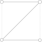
Example 3.1.
Let us consider the homeomorphism defined by , which dilates the interior of the square while keeping the diagonal fixed. Furthermore, restricted to the incomplete subcomplex shown in Figure 1, is also a homeomorphism. A simplicial approximation of is the identity, so in this case, it holds
3.2. Definition of the combinatorial Lefschetz number
We now address the definition of the combinatorial Lefschetz number.
Definition 3.2.
Let be a homeomorphism of a simplicial complex to itself. Let be a definable -invariant set. Let be its closure in . We define as , where is the map induced by in a triangulation of compatible with (the existence of this triangulation guaranteed by Theorem 2.2). We will say that is the combinatorial Lefschetz number of in relative to .
Remark 3.3.
Under the above conditions, can be extended to a homeomorphism of to itself, so that we can consider . We will see that, in this case, . In particular, for any extension of to , in fact
Note that the use of is a small abuse of notation since is not a simplicial complex. Actually, we would have to write instead of .
Definition 3.4.
Under the conditions of Definition 3.2, let be defined as , where is a simplicial approximation of in (with respect to a possibly finer simplicial structure in ).
Remark 3.5.
Let be the triangulation compatible with , and chosen in Definition 3.2. Since is -invariant, we have , and therefore . Furthermore, since is definable, we have that is definable, and, since is homeomorphism, is also -invariant. Thus, since , it follows that is -invariant and definable ( is definable because it is the closure of a definable (see [13, Lemma 3.4, Chapter 1]).
Consequently, since is a homeomorphism, and are -invariant (they are definable because they are unions of open simplices). Also, again, since is a homeomorphism, , which is a simplicial (complete) subcomplex of .
Remark 3.6.
Under the conditions of Definition 3.2, note that, since is -invariant, maps chains of to chains of . Furthermore, if is a simplicial approximation of , then is a simplicial approximation of , which suggests that can be equal to .
Remark 3.7.
In there does not have to exist a simplicial approximation of , but there does exist such a simplicial approximation between a subdivision of and . Then, it is simply needed to compose with the subdivision operator [10, Theorem 17.2]. Really, we are using an abuse of notation in Definition 3.4. What is called simplicial approximation is actually a modification of it so that the domain and co-domain coincide, and induces in homology the map in order to use the Hopf’s trace theorem.
It remains to define .
Definition 3.8.
Let be a simplicial chain map. Let be an incomplete subcomplex or a disjoint and finite union of them. In each dimension , the simplicial chains have the base of oriented -symplices of . Likewise, maps -chains to -chains. In each dimension , we will said that an incomplete basis of W consists of the -simplices such that is an open simplex of . Thus, we can restrict the matrix of the map to the square submatrix of coefficients such that and belong to the incomplete basis of . Then is defined as the alternating sum of the traces of these submatrices in the different dimensions of the complex .
3.3. Well-definess of combinatorial Lefschet number
Let us see below that Definition 3.2 is consistent. In the case of the combinatorial Euler characteristic, this was done in [2, 9].
Theorem 3.9.
Under the conditions of Definition 3.2, the combinatorial Lefschetz number is well defined.
In order to prove the theorem, we must do the following:
-
(a)
To prove that .
-
(b)
To check that, if and are two triangulations of compatible with , and , and and are the maps induced on them by then .
-
(c)
To show that when and are two simplicial approximations of (defined on simplicial structures of which may be different).
Let us begin by showing c.
Lemma 3.10.
Let be a simplicial complex and a homeomorphism. Let be a definable and -invariant subspace. Let be a triangulation of compatible with , and , and let be the map induced by in . Let and be two simplicial approximations of . Then .
Proof.
As we already mentioned in Remark 3.5, and are -invariant. Additionally, and map chains of to chains of (Remark 3.6). Note also that is a finite (disjoint) union of incomplete complexes (in particular, it is an incomplete complex) but is a complete subcomplex of (this is why we defined the combinatorial Lefschetz number relative to a complete simplicial complex, since if were not a complete complex, would not have to be a complete simplicial complex).
The proof is made by recurrence.
Due to the definition of , we have:
(Note that satisfies the conditions of Definition 3.8, so it makes sense to consider .)
Now, by the Hopf trace theorem [10, Theorem 22.1], since and are simplicial approximations of , we have
On the other hand, note that we can repeat the process considering instead of , since is a complete complex -invariant, and map chains of to chains of and are simplicial approximations of , and satisfies the conditions of Definition 3.8. In this way, we get
Again, note that
Now, with the recurrence process, the dimension of the complexes becomes smaller since Eventually, the dimension of the first term on the right-hand side of the equalities is zero. Then that complex, denoted by , is a finite union of points ,and thus . In that case,
and, going back in every dimension, we get
Now let us prove b.
Lemma 3.11.
Let be a simplicial complex and a homeomorphism. Let be a definable -invariant subset. Let and be two triangulations of compatible with , and , and let and be the maps induced by on and , respectively. Then .
Proof.
Again, a triangulation is supported by , , …, and also
Finally, (respectively, ), , … are complete and -invariant (respectively, -invariant) complexes. So (respectively, ) maps chains of , , … to chains of , , …
We argue by recurrence. On the one hand, we have:
Note that we have already seen that the numbers on the left of the equality will not depend on the simplicial approximation chosen. Since
and the same for , we get:
Now, since and are homeomorphic, we get because, by the Hopf’s trace theorem,
and by [10, Section 22], we have , obtaining .
Again, and are in the same conditions as and . So, repeating the above argument, we get
And again, by [10, Theorem 22.1 and Section 2], we have . By repeating this process, eventually the dimension of the first member on the right of the equality is zero, and therefore the Lefschetz numbers are equal for and . Hence, . ∎
4. Properties and consequences
We derive some properties of the combinatorial Lefschetz number which we will use later. Moreover, we derive a fixed point theorem.
4.1. Additivity. Inclusion-Exclusion. Product property.
Note that the combinatorial Lefschetz number is additive in the sense that, if and are two disjoint definable and -invariant subsets of a simplicial complex , then . More generally, if and are non disjoint, then:
Moreover, it holds a product property.
Theorem 4.1 (Product property of the combinatorial Lefchetz number).
Let be a homeomorphism of a complete simplicial complex to itself. Let be definable sets such that , , , and , where and are homeomorphisms whose restrictions to and are also homeomorphisms. Then
| (4) |
Remark 4.2.
Although it seems to be very restrictive hypotheses to require that , , remain homeomorphisms, note that they are locally satisfied in the case of bundles.
On the other hand, neither nor have to be simplicial complexes, so (resp. ) do not have to be defined. Actually, in (4) an abuse of notation is being committed, writing instead of the complex to which the triangulation of leads.
Proof.
Let be a triangulation compatible with . Since the following diagram commutes
it follows that and . Analogously, we see that and .
Note that , and are triangulations of , and , respectively. Thus, .
Let us check then that . For this purpose, we triangulate by , obtaining
We will then see that
Now, in order to triangulate by , we first need to be a complex simplicial. This is achieved since both and are complete simplicial complexes, by taking as new vertices pairs consisting of barycenters of original simplices. Furthermore, since this procedure respects the incomplete subcomplexes of and , we have
| (5) |
Now, from the product rule for the Lefschetz number: .
Note now that, since , , , are homeomorphisms, we get that and are also homeomorphisms, and therefore , and are homeomorphisms. Let us study for example . Note that the dimension of is strictly smaller than that of . Furthermore, reproducing the argument used for (since all of the hypotheses are met), we have
By repeating this process, the last three terms eventually are of dimension zero, and therefore they are complete complexes, for which we can apply the product formula. As an illustrative example, suppose that , and are of dimension zero. Then
But, on the other hand,
Now, combining both equalities, we get
where the last equality follows from .
In this way, if we go up in dimension until we reach (5), we have
and, again, decomposing into four terms, we obtain
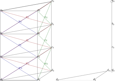
Example 4.3.
Let us consider the hollow simplicial complex shown in Figure 2. Let be the incomplete subcomplex resulting from multiplying the open subcomplex by the open subcomplex . Let now be the map resulting from turning degrees over the axis . It is a simplicial map. Moreover, subcomplex is -invariant and , where is the reflection over the vertex and is the reflection over the midpoint of the segment. If we compute now , and we obtain:
4.2. Fixed point property for the combinatorial Lefschetz number
Once the combinatorial Lefschetz number is defined, we can obtain a fixed point theorem that generalizes the fixed point theorem of the Lefschetz number.
Theorem 4.4 (Generalised fixed point theorem).
Let be a complete and finite simplicial complex, and let be a homeomorphism. Suppose is a definable and -invariant subset. If , then has a fixed point in .
Proof.
We only sketch the idea of the proof since it is analogous to the classical one. If doesn’t have any fixed point in we could take a sufficiently small distance for which any -ball in would not have any fixed point. Taking a small barycentric subdivision (of diameter quite smaller than ) and a simplicial approximation of , will not carry any simplex of the barycentric subdivision into itself, and so so the combinatorial Lefschetz number will be zero. ∎
We present two examples of the fixed point property of the combinatorial Lefschetz number. In the first one is interesting because shows an example of a map that has a fixed point only in the boundary of the definable set studied. On the other hand, the second example presents a case where we will not be able to apply the traditional Lefschetz fixed point because it is zero.
Example 4.5.
In the first one, we have the complex and the map . If we consider , we see that but f only has fixed points in the boundary of the interval.

5. Integral with respect to the Lefschetz number
We have already defined a combinatorial Lefschetz number, which, in a sense, is invariant by homeomorphisms (if they can be extended to the closure of the space). Let us now define an integral with respect to this number.
Definition 5.1.
Let be a homeomorphism of a simplicial complex to itself. Let be sets in the algebra of definable and -invariant sets. We define
Likewise, we will say that a function is -integrable if admits an expression of the form , with the in the mentioned algebra of sets.
Theorem 5.2.
The integral with respect to the Lefschetz number is well defined. Furthermore, it satisfies
where .
Proof.
Let , with and in the conditions of Definition 5.1. Let us check that
Let if and if . Let us now consider a triangulation of compatible with every and with
| (6) |
(Actually, since is bijective, it is enough for the triangulation to be compatible with the .)
Now, these last sets belong to the algebra of definable and -invariants sets, and, furthermore, each can be written as a disjoint union of some of them. Let denote the images of the and the sets of (6) by the triangulation. So,
where .
Analogously, we get
Now, since , we obtain, for all ,
Thus, the integral with respect to the Lefschetz number is well defined. The second part of the proof is a straightforward verification. ∎
6. Product rule and Fubini theorem
At this point, we are interested in obtaining applications of the Lefschetz number that we have just defined. First of all, we will try to take advantage of the measure defined in the Definition 5.1. Precisely, first we will obtain a combinatorial Lefschetz number rule for the product of definable sets. Once obtained this rule, we will state and prove a Fubini Theorem, the generalization in measure language of the product rule for the case of triangulable bundles, in a similar way as in [4, Theorem 4.5].
6.1. Fubini Theorem
Before proving Fubini’s theorem, for our theory of integration, we need two previous lemmas.
Lemma 6.1.
Let be a fiber bundle with a simplicial complex. Then, for each , there exists a definable open neighborhood such that .
Proof.
Since is a fiber bundle, we know that there exists an open neighborhood of such that . Let be the intersection of an open cell with (in particular, a definable subset) of such that its closure is contained in (its existence is given by normality). Thus, since because is a fiber bundle, it follows that
Lemma 6.2.
Let be a fiber bundle with typical fiber , where is definable, and , and are complete simplicial complexes. Let so that and . Let be defined as . Let be a homeomorfism such that and are -invariant and and , with , , and . Then
| (7) |
Remark 6.3.
In (7), refers to the map that it induces in every fiber .
Proof.
We have
Remark 6.4.
Based on Lemma 6.2, let us now formulate and prove a Fubini theorem. Before, note that, since is compact (it is a finite complex), it admits a finite covering with the of the form of Lemma 6.1, which, in turn, induces a covering of formed by . Thus, we can apply our Fubini theorem to applications that locally are of the form .
Theorem 6.5 (Fubini Theorem for Lefschetz integration).
Let be a fiber bundle such that , and finite simplicial complexes, and is definable. Let be the covering as in Remark 6.4. Let be a homeomorfism such that and , with . Then
Proof.
Because -integrable, , where is -invariant and definable. Then
Now, by Lemma 6.2, the last term can be written as
7. Application to counting methods
In [4], the application of the combinatorial Euler characteristic to counting methods using sensors was already studied. We will generalize part of his results in the same way that the Lefschetz number generalizes to the Euler characteristic.
Let us imagine that we have sensors on the floor of a building so that we can assume that there is a sensor at every point of the floor. Suppose that every person (denoted by ) in the building activates the sensors in a neighborhood. In this way, we can define a counting function that, for each sensor, tells us the number of people it detects. In this case, we have the following result.
Theorem 7.1 (Counting Theorem).
Let be a counting function. If there exists an homeomorphism such that , where every is definable and -invariant, and with , then
Proof.
Remark 7.2.
The above theorem is not a crude generalization of the result presented in [4]. Indeed, we can find simple examples in which the identity map does not allow us to count the number of people but other homeomorphisms, such as a reflection, do. In the following example, we present one of these cases.
Example 7.3.
Let us consider the simplicial complex shown in Figure 4.
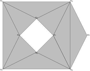
Let be the function that has the value at the closed simplex , and the value at the rest of the complex. This function can be written as the sum of the characteristic function of the subcomplex generated by the vertices and the characteristic function of the subcomplex generated by the vertices . Both subcomplexes are invariant by the reflection with respect to the axis containing the vertices , and , but their Euler characteristics are different.
The applications of this counting method are diverse. Like systems that allow us to count the number of passengers in stations, shopping centers or airports, or mechanisms that indicate the number of fish in a fish farm.
References
- [1] M. Arkowitz, R. Brown (2004). The Lefschetz-Hopf theorem and axioms for the Lefschetz number, Fixed Point Theory Appl., (1), 1–11.
- [2] T. Beke (2011). Topological invariance of the combinatorial Euler characteristic of tame spaces, Homology, Homotopy and Applications, (13), 2, 165–174.
- [3] W. Blaschke (1936). Vorlesungen über Integralgeometrie, Vol. 1, 2nd edition. Leipzig and Berlin, Teubner.
- [4] J. Curry, R. Ghrist and M. Robinson (2012). Euler calculus with applications to signals and sensing, Proceedings of Symposia in Applied Mathematics, (70), 75–146.
- [5] Y. Baryshnikov, R. Ghrist (2009).Target enumeration via Euler characteristic integrals, SIAM Journal on Applied Mathematics, (70), 3, 825–844.
- [6] M. Kashiwara, Index theorem for maximally overdetermined systems of linear differential equations, Proc. Japan Acad. Ser. A Math. Sci., 49 (10), 1973, 803–804.
- [7] S. MacLane, (1963). Homology, Springer-Verlag, Berlin and New York.
- [8] R. MacPherson, Chern classes for singular algebraic varieties, Ann. of Math. 100, 1974, 423–432.
- [9] C. McCrory, A. Parusinski (1997). Algebraically constructible functions, Ann. Sci. École Norm. Sup., (4), 30, 527–552.
- [10] J. R. Munkres (1984). Elements of Algebraic Topology, Addison-Wesley, Cambridge Massachusetts.
- [11] H. Putz, (1967). Triangulation of Fibre Bundles. Canadian Journal of Mathematics, 19, 499–513.
- [12] P. Schapira, Operations on constructible functions, J. Pure Appl. Algebra, 72, 1991, 83–93.
- [13] L. P. D. van der Dries (2009). Tame Topology and O-minimal Structures, Cambridge University Press.