E-values, Multiple Testing and Beyond

Abstract

We discover a connection between the Benjamini-Hochberg (BH) procedure and the recently proposed e-BH procedure Wang and Ramdas (2022) with a suitably defined set of e-values. This insight extends to a generalized version of the BH procedure and the model-free multiple testing procedure in Barber and Candès (2015) (BC) with a general form of rejection rules. The connection provides an effective way of developing new multiple testing procedures by aggregating or assembling e-values resulting from the BH and BC procedures and their use in different subsets of the data. In particular, we propose new multiple testing methodologies in three applications, including a hybrid approach that integrates the BH and BC procedures, a multiple testing procedure aimed at ensuring a new notion of fairness by controlling both the group-wise and overall false discovery rates (FDR), and a structure adaptive multiple testing procedure that can incorporate external covariate information to boost detection power. One notable feature of the proposed methods is that we use a data-dependent approach for assigning weights to e-values, significantly enhancing the efficiency of the resulting e-BH procedure. The construction of the weights is non-trivial and is motivated by the leave-one-out analysis for the BH and BC procedures. In theory, we prove that the proposed e-BH procedures with data-dependent weights in the three applications ensure finite sample FDR control. Furthermore, we demonstrate the efficiency of the proposed methods through numerical studies in the three applications.

Keywords: Benjamini-Hochberg procedure, Cross-fitting, E-values, False discovery rate, Leave-one-out analysis, Multiple testing

1 Introduction

When working with high-dimensional data in modern scientific fields, the problem of multiple testing often arises when we explore a vast number of hypotheses with the goal of detecting signals while also controlling some error measures, such as the false discovery rate (FDR). The Benjamini-Hochberg (BH) procedure (Benjamini and Hochberg, 1995) is perhaps the most widely used FDR-controlling procedure that rejects a hypothesis whenever its p-value is less than or equal to an adaptive rejection threshold determined by the whole set of p-values. Barber and Candès (2015) proposed a model-free FDR-controlling (BC) procedure that estimates the number of false rejections by leveraging the symmetry of p-values under the null and compares each p-value with an adaptive threshold. More recently, there is a growing literature on utilizing e-values for statistical inference under different contexts, see, e.g., (Grünwald et al., 2020; Shafer, 2021; Vovk and Wang, 2021; Xu et al., 2021; Ignatiadis et al., 2022; Dunn et al., 2023; Xu and Ramdas, 2023). In particular, Wang and Ramdas (2022) proposed a multiple testing procedure (named e-BH procedure) by applying the BH procedure to e-values, which was shown to control the FDR even when the e-values exhibit arbitrary dependence.

In this work, we establish a connection between the BH and e-BH procedures with a suitably defined set of e-values, proving that they yield identical rejection sets. This connection extends to a generalized version of the BH and BC procedures, which can have a more general form for the rejection rule. Based on these findings, we propose new multiple testing procedures by aggregating e-values from the BH and BC procedures or assembling e-values from different subsets of the data. Specifically, we consider three concrete applications, which we will illustrate in detail below.

Our first application concerns the development of a robust and efficient multiple testing procedure by leveraging the strength of the BH and BC procedures. The BH and BC procedures employ different strategies to estimate the number of false rejections, leading to distinct performances depending on the underlying signal density and strength. Empirical results in the literature suggest that neither one dominates the other. For instance, the BH procedure is usually more powerful when the underlying signal is sparse, while the BC procedure excels in the case of dense signal (Arias-Castro and Chen, 2017). It is often impossible to know in advance which method will perform better in real-world applications. Reporting results from the better-performing method can lead to an inflated FDR and is considered as a type of data snooping. To develop a more efficient procedure with guaranteed FDR control, we propose a hybrid method that utilizes e-values as a bridge to integrate the testing results from the BH and BC procedures. Specifically, we construct a set of e-values by properly weighting the e-values from both the BH and BC procedures. We then use the constructed e-values as the input for the e-BH procedure. We show that the resulting hybrid procedure controls the FDR and can significantly improve the worse-performing method in finite sample.

Our second application is concerned with a setting where one has to make (high-stakes) decisions by testing $n$ hypotheses that are partitioned into $G$ groups according to some (protected) attributes. Let us consider the example of a bank’s loan approval process, where customers are grouped by gender or race. The null hypothesis in this case is that the loan should be approved for the customer. The bank faces the challenge of controlling the overall FDR, which means that the bank should not falsely decline too many customers’ applications, as it would reduce the loan volume and decrease income. Additionally, the bank also needs to control the group-wise FDR to ensure that certain racial or gender groups are not unfairly denied loans. If the group-wise FDR inflates, customers who believe they are unfairly denied loans may take their business elsewhere. Therefore, the bank aims to maintain control over the FDR for each group while also controlling the overall FDR across all hypotheses. Applying an FDR-controlling procedure to the whole set of hypotheses, ignoring the group structure will fail to control the FDR for individual groups. On the other hand, performing multiple testing for each group separately at level $\alpha$ does not ensure that the overall FDR is controlled at the same level $\alpha$. A naive procedure to achieve error control at both the group and overall levels is to conduct multiple testing for each group separately at the reduced level $\alpha/G$, which turns out to be too conservative, as seen in our (unreported) numerical studies. To address this challenge, we propose a fair multiple testing procedure that uses e-values as a bridge to assemble the results from different groups, controlling the FDR within each group and the overall FDR simultaneously. Specifically, we implement the BC procedure for each group, followed by constructing e-values by assembling e-values from different groups with proper weights, and using the constructed e-values as the input for the e-BH procedure. We show that the resulting procedure simultaneously controls the FDR within each group and the overall FDR in finite sample.

As the final application, we consider the problem of multiple testing with external structural information in the form of covariates, which has received much recent attention, as leveraging auxiliary information can enhance the power and interpretability of multiple testing results in many scientific applications. For instance, in differential expression analysis of RNA-seq data, which tests for differences in the mean expression of the genes between conditions, the sum of read counts per gene across all samples could be the auxiliary data since it is informative of the statistical power. In differential abundance analysis of microbiome sequencing data, which tests for differences in the mean abundance of the detected bacterial species between conditions, the genetic divergence among species is important auxiliary information since closely related species usually have similar physical characteristics and tend to covary with the condition of interest. A growing list of works has reflected the importance of this research direction in recent years, for instance, (Genovese et al., 2006; Hu et al., 2010; Sun et al., 2015; Ignatiadis et al., 2016; Boca and Leek, 2018; Lei and Fithian, 2018; Li and Barber, 2019; Ignatiadis and Huber, 2021; Yun et al., 2022; Zhang and Chen, 2022; Zhao and Zhou, 2023). However, these existing works suffer from different limitations. For example, the local FDR-based method (Sun et al., 2015; Cao et al., 2022) lacks finite sample FDR control and can only guarantee FDR control asymptotically. The weighted BH methods (Ignatiadis and Huber, 2021; Li and Barber, 2019) lead to suboptimal power, as observed in our numerical studies. To address these drawbacks, we propose a powerful multiple testing procedure that incorporates auxiliary information with guaranteed FDR control in finite samples. We randomly split samples into several groups and use the cross-fitting approach to estimate the rejection function in each group using all samples in other groups. Then, we implement the generalized BC procedure for each group. We assemble the BC procedure induced e-values from different groups with proper weights. The assembled e-values are used as the input for e-BH procedure. We show that the proposed procedure controls the FDR at the desired level in finite sample.

Our approach involves a data-dependent method for weighting e-values when aggregating them from the BH and BC procedures (the first application) or assembling them from different subsets of the data (the second and third applications). It is important to note that our weighting method differs from the “boosting factor” proposed by Wang and Ramdas (2022), which involves multiplying each e-value by a factor to boost them up before applying the e-BH procedure. In our approach, we construct weights that ensure the weighted e-values satisfying Condition (3) below. This condition is sufficient to maintain FDR control of the e-BH procedure at the desired level. Our numerical findings show that implementing the e-BH procedure with data-dependent weights improves its efficiency across all applications compared to the unweighted e-BH procedure.

The rest of the paper is organized as follows. In Section 2, we provide a brief review of the BH, BC, and e-BH procedures and establish the equivalence between the BH/BC and the e-BH procedures. In Section 3, we extend this equivalence to a generalized version of the BH and BC procedures. We present new multiple testing methodologies in three different applications, including a hybrid approach that integrates the BH and BC procedures, a multiple testing procedure that controls both the group-wise and overall FDRs, and a structure adaptive multiple testing procedure, in Sections 4.1, 4.2, and 4.3, respectively. Section 5 concludes. The appendix contains additional numerical results and all proofs of the main results.

2 Preliminaries

To begin with, we provide a brief overview of the BH, BC, and e-BH procedures, and establish the equivalence between the BH (BC) procedure and the e-BH procedure with a suitably defined set of e-values. This equivalence appears to be a new finding that has not been explicitly stated in the previous literature.

We are interested in testing $n$ hypotheses $\{H_{1},\dots,H_{n}\}$ simultaneously. Let $\bm{\theta}=\{\theta_{1},\dots,\theta_{n}\}\in\{0,1\}^{n}$ indicate the underlying truth of each hypothesis, where $\theta_{i}=0$ if $H_{i}$ is under the null and $\theta_{i}=1$ otherwise. Denote by $\bm{\delta}=(\delta_{1},\dots,\delta_{n})\in\{0,1\}^{n}$ a decision rule for the $n$ hypotheses, where we reject (accept) the $i$th hypothesis if $\delta_{i}=1$ ($\delta_{i}=0$). The FDR for the decision rule $\bm{\delta}$ is defined as the expectation of the false discovery proportion (FDP), i.e.,

$$\mathrm{FDR}(\bm{\delta})=\mathbb{E}[\mathrm{FDP}(\bm{\delta})],\quad\mathrm{FDP}(\bm{\delta})=\frac{\sum_{i=1}^{n}(1-\theta_{i})\delta_{i}}{1\vee\sum_{i=1}^{n}\delta_{i}},$$

where $a\vee b=\max\{a,b\}$. The goal of an FDR controlling procedure is to ensure that the FDR is bounded from above by a pre-specified number $\alpha\in(0,1)$.

2.1 BH procedure

The Benjamini-Hochberg (BH) procedure (Benjamini and Hochberg, 1995) is perhaps the most widely used FDR-controlling method. To describe the procedure, suppose we observe a p-value $p_{i}$ for each $H_{i}$. Sort the p-values in ascending order as $p_{(1)}\leq\dots\leq p_{(n)}$ and let $\hat{k}=\max\left\{i\colon p_{(i)}\leq(\alpha i)/n\right\}$. The BH procedure rejects all hypotheses $H_{(i)}$ with $i\leq\hat{k}$, where $H_{(i)}$ is the hypothesis associated with $p_{(i)}$. This procedure is equivalent to rejecting all $H_{i}$ with $p_{i}\leq T_{\mathrm{BH}}$, where $T_{\mathrm{BH}}$ is defined as

$$T_{\mathrm{BH}}=\sup\left\{0<t\leq 1\colon\frac{nt}{1\vee R(t)}\leq\alpha\right\},$$ (1)

with $R(t)=\sum_{i=1}^{n}\mathbbm{1}\{p_{i}\leq t\}$ being the number of rejections given the threshold $t$, and $\mathbbm{1}\{A\}$ denoting the indicator function associated with a set $A$. It is well known that if the null p-values are mutually independent and super-uniform, and are independent of the alternative p-values, the BH procedure at level $\alpha$ controls the FDR at the level $\alpha n_{0}/n\leq\alpha$, where $n_{0}$ is the number of hypotheses under the null.

2.2 BC procedure

In a seminal paper by (Barber and Candès, 2015), the authors proposed a model-free multiple testing procedure (BC procedure hereafter) that exploits the symmetry of the null p-values (or test statistics) to estimate the number of false rejections. More precisely, the BC procedure specifies a data-dependent threshold, denoted by $T_{\mathrm{BC}}$, which is determined as follows:

$$T_{\mathrm{BC}}=\sup\left\{0<t<0.5\colon\frac{1+\sum^{n}_{i=1}\mathbbm{1}\{p_{i}\geq 1-t\}}{1\vee R(t)}\leq\alpha\right\},$$ (2)

and it rejects all $H_{i}$ with $p_{i}\leq T_{\mathrm{BC}}$. The BC procedure has been shown to provide finite sample FDR control under suitable assumptions (Barber and Candès, 2015).

2.3 E-values and e-BH procedure

A non-negative random variable $E$ is called an e-value if $\mathbb{E}[E]\leq 1$ under the null hypothesis. Suppose we observe $n$ e-values $e_{1},\dots,e_{n}$ corresponding to the hypotheses $H_{1},\dots,H_{n}$. The $\alpha$-level e-BH procedure involves sorting the e-values in decreasing order as $e_{(1)}\geq\dots\geq e_{(n)}$ and rejecting the hypotheses associated with the $\hat{k}$ largest e-values, where $\hat{k}\coloneqq\max\left\{1\leq i\leq n\colon e_{(i)}\geq n/(i\alpha)\right\}$.

Proposition 1 (Theorem 2 of Wang and Ramdas (2022)).

Suppose the e-values satisfy

$$\sum_{i\in\mathcal{H}_{0}}\mathbb{E}[e_{i}]\leq n,$$ (3)

where $\mathcal{H}_{0}=\{1\leq i\leq n:\theta_{i}=0\}$. Then, the $\alpha$-level e-BH procedure controls the FDR at the level $\alpha$, regardless of the dependence structure among the e-values.

2.4 Connection between the BH and e-BH procedures

To see the connection between the BH and e-BH procedures, we define the e-value associated with $H_{i}$ to be

$$e_{i}=T_{\mathrm{BH}}^{-1}\mathbbm{1}\{p_{i}\leq T_{\mathrm{BH}}\},$$ (4)

where $T_{\mathrm{BH}}$ is given in (1). By Lemmas 3-4 in Storey et al. (2004), $\sum_{i\in\mathcal{H}_{0}}\mathbbm{1}\{p_{i}\leq t\}/t$ for $0<t\leq 1$ is martingale with time running backwards with respect to the filtration $\mathcal{F}_{t}=\sigma(\mathbbm{1}\{p_{i}\leq s\}:t\leq s\leq 1,i=1,2,\dots,n)$, and $T_{\mathrm{BH}}$ is a stopping time with respect to $\mathcal{F}_{t}$, where $\mathcal{F}_{t}$ is the sigma field generated by $\mathbbm{1}\{p_{i}\leq s\}$ for $t\leq s\leq 1.$ By the optional stopping time theorem, we have

$$\sum_{i\in\mathcal{H}_{0}}\mathbb{E}[e_{i}]=\mathbb{E}\left[\frac{\sum_{i\in\mathcal{H}_{0}}\mathbbm{1}\{p_{i}\leq T_{\mathrm{BH}}\}}{T_{\mathrm{BH}}}\right]=\mathbb{E}\left[\sum_{i\in\mathcal{H}_{0}}\mathbbm{1}\{p_{i}\leq 1\}\right]=n_{0},$$

which implies that the e-values defined by equation (4) satisfy (3). Thus by Proposition 1, the corresponding e-BH procedure controls the FDR at the desired level. Moreover, we claim that the e-BH procedure based on the e-values defined in (4) is equivalent to the BH procedure based on $\{p_{1},\dots,p_{n}\}$ in the sense that they produce the same set of rejections.

Theorem 1.

Let $\mathcal{S}_{\mathrm{BH}}$ be the set of rejections obtained through the BH procedure at the FDR level $\alpha$, and let $\mathcal{S}_{\mathrm{eBH}}$ represent the set of rejections obtained from the e-BH procedure at the same FDR level $\alpha$, with the e-values defined in (4). Then we have $\mathcal{S}_{\mathrm{BH}}=\mathcal{S}_{\mathrm{eBH}}$.

2.5 Connection between the BC and e-BH procedures

As noted in a recent work by Ren and Barber (2022), the BC procedure is equivalent to the e-BH procedure based on the following e-values:

$$e_{i}=\frac{n\mathbbm{1}\{p_{i}\leq T_{\mathrm{BC}}\}}{1+\sum_{j=1}^{n}\mathbbm{1}\{p_{j}\geq 1-T_{\mathrm{BC}}\}},$$

where $T_{\mathrm{BC}}$ is the threshold defined in (2).

3 Generalized BH and BC procedures

In this section, we extend the BH and BC procedures to allow a general class of rejection rules. This generalization enables the testing procedure to utilize cross-sectional information among the p-values and external structural information for each hypothesis, which often results in a higher multiple testing power. We shall establish the connection between these generalized procedures and the corresponding e-BH procedures.

3.1 Generalized BH procedure

We generalize the BH procedure to allow the rejection rule to take the form of $\varphi_{i}(p_{i})\leq t$, where $\varphi_{i}$ is a strictly increasing function and can differ for each $i$. Let us define $F_{i}(t)=\varphi_{i}^{-1}(t)$ as the inverse function of $\varphi_{i}$, and consider the rejection threshold

$$T_{\text{GBH}}=\sup\left\{0<t\leq 1:\frac{\sum^{n}_{i=1}F_{i}(t)}{1\vee R(t)}\leq\alpha\right\},$$ (5)

where $R(t)=\sum^{n}_{i=1}\mathbbm{1}\{\varphi_{i}(p_{i})\leq t\}$. The generalized BH (GBH) procedure rejects $H_{i}$ whenever $\varphi_{i}(p_{i})\leq T_{\mathrm{GBH}}$. Similar to the BH procedure, the GBH procedure can be equivalently implemented in the following way. Define $\bar{F}(t)=n^{-1}\sum^{n}_{i=1}F_{i}(t)$ which is strictly increasing in $t$. We sort $q_{i}=\varphi_{i}(p_{i})$ in an ascending order, i.e., $q_{(1)}\leq\dots\leq q_{(n)}$ and find the largest $k$, represented as $\hat{k}$, for which $q_{(k)}\leq\bar{F}^{-1}\left(\frac{\alpha k}{n}\right).$ We then reject $H_{(i)}$ for all $i\leq\hat{k}$. The following proposition states that, under appropriate conditions in the form of $F_{i}$, the GBH procedure ensures FDR control.

Proposition 2.

Suppose that the null p-values $\{p_{i}\}_{i\in\mathcal{H}_{0}}$ are mutually independent and super-uniform, and are independent of the alternative p-values $\{p_{i}\}_{i\notin\mathcal{H}_{0}}$. If $F_{i}(t)=c_{i}h(t)$ where $c_{i}$ is some constant and $h$ is a strictly increasing function of $t$, the GBH procedure controls the FDR at level $\alpha$.

As illustrated in the following examples, the GBH procedure aligns with several methods in the literature of structure adaptive multiple testing.

Example 1.

Let $\varphi_{i}(p)=p/\omega_{i}$, where $\omega_{i}$ denotes the weight for the $i$th hypothesis with $\omega_{i}>0$ and $\sum_{i=1}^{n}\omega_{i}=n$. The GBH procedure associated with this choice of $\varphi_{i}$ corresponds to the weighted BH procedure first introduced by Genovese et al. (2006). In this case, $F_{i}(t)=w_{i}t$ and the rejection threshold can be expressed as

$$T_{\text{GBH}}=\sup\left\{0<t\leq 1\colon\frac{\sum_{i=1}^{n}w_{i}t}{1\vee R(t)}\leq\alpha\right\}=\sup\left\{0<t\leq 1\colon\frac{nt}{1\vee R(t)}\leq\alpha\right\},$$

where $R(t)=\sum_{i=1}^{n}\mathbbm{1}\{p_{i}/w_{i}\leq t\}$.

Example 2.

Another choice of $\varphi_{i}$ is the local FDR (Efron, 2005; Sun and Cai, 2007) under a two-group mixture model. Specifically, we assume that the p-values are independently generated from the mixture density given by $\pi_{i}+(1-\pi_{i})(1-\kappa)p^{-\kappa}$, where $\pi_{i}\in(0,1)$ is the mixing proportion and $\kappa\in(0,1)$ controls the shape of the p-value density under the alternative. The rejection rule based on the local FDR under this model is given by

$$\varphi_{i}(p)=\frac{\pi_{i}}{\pi_{i}+(1-\pi_{i})(1-\kappa)p^{-\kappa}}\leq t,$$ (6)

which is the probability that the $i$th hypothesis is under the null given the observed p-value being $p$. It follows that

$$F_{i}(t)=\varphi_{i}^{-1}(t)=\left(\frac{\pi_{i}(1-t)}{(1-\pi_{i})t(1-\kappa)}\right)^{-1/\kappa}=c_{i}h(t),$$

where $c_{i}=\left\{\pi_{i}/\bigl{(}(1-\pi_{i})(1-\kappa)\bigr{)}\right\}^{-1/\kappa}$ and $h(t)=\left\{(1-t)/t\right\}^{-1/\kappa}$.

3.2 Connection between the GBH and e-BH procedures

Analogous to the BH procedure, we show that the GBH procedure is equivalent to the e-BH procedure applied to the following e-values:

$$e_{i}=\frac{n\mathbbm{1}\{\varphi_{i}(p_{i})\leq T_{\text{GBH}}\}}{\sum^{n}_{i=1}F_{i}(T_{\mathrm{GBH}})},$$ (7)

where $T_{\text{GBH}}$ is defined in (5). By the leave-one-out argument, we prove the following result.

Proposition 3.

Under the assumptions in Proposition 2, the e-values $e_{1},\dots,e_{n}$ defined in (7) satisfy Condition (3). As a consequence, the corresponding e-BH procedure controls the FDR at the desired level.

Additionally, we can prove that the e-BH procedure and the GBH procedure deliver the same set of rejections.

Theorem 2.

Let $\mathcal{S}_{\mathrm{GBH}}$ be the set of rejections obtained through the GBH procedure at the FDR level $\alpha$, and let $\mathcal{S}_{\mathrm{eBH}}$ represent the set of rejections obtained from the e-BH procedure at the same FDR level $\alpha$, with the e-values defined in (7). Then we have $\mathcal{S}_{\mathrm{GBH}}=\mathcal{S}_{\mathrm{eBH}}$.

3.3 Generalized BC procedure

In this section, we generalize the BC procedure with the rejection rule given by $\varphi_{i}(p_{i})\leq t$. We assume that the null p-value satisfies the following condition:

$$P(p_{i}\leq a)\leq P(p_{i}\geq 1-a)=P(1-p_{i}\leq a),\quad\text{ for all }0\leq a\leq 0.5.$$ (8)

Condition (8) is weaker than the mirror conservativeness in Lei and Fithian (2018), and it can be shown that super-uniformity implies (8). Indeed,

$$P(1-p_{i}\leq a)\geq 1-P(p_{i}\leq 1-a)\geq 1-(1-a)=a\geq P(p_{i}\leq a).$$

Assume that $\varphi_{i}$ is an increasing and continuous function, and define $F_{i}(x)=\sup\{0\leq p\leq 1\colon\varphi_{i}(p)\leq x\}$. We claim that

$$P(\varphi_{i}(p_{i})\leq b)=P(p_{i}\leq F_{i}(b)).$$

To see this, consider two cases. If $\varphi_{i}(p_{i})\leq b$, by the definition of $F_{i}(b)$, we have $p_{i}\leq F_{i}(b)$. On the other hand, if $p_{i}\leq F_{i}(b)$, then $\varphi_{i}(p_{i})\leq\varphi_{i}(F_{i}(b))=\lim_{p\uparrow F_{i}(b)}\varphi_{i}(p)\leq b$, where we use the fact that $\varphi_{i}$ is increasing to get the two inequalities, and the equality is due to the continuity of $\varphi_{i}$. Therefore, the above claim together with equation (8) implies that

$$P(\varphi_{i}(p_{i})\leq b)=P(p_{i}\leq F_{i}(b))\leq P(1-p_{i}\leq F_{i}(b))=P(\varphi_{i}(1-p_{i})\leq b),$$ (9)

for all $\varphi_{i}(0)\leq b\leq\varphi_{i}(0.5)$. Hence, we have

$$\frac{\sum_{i\in\mathcal{H}_{0}}\mathbbm{1}\{\varphi_{i}(p_{i})\leq t\}}{1\vee\sum_{i=1}^{n}\mathbbm{1}\{\varphi_{i}(p_{i})\leq t\}} \approx\frac{\sum_{i\in\mathcal{H}_{0}}P(\varphi_{i}(p_{i})\leq t\})}{1\vee\sum_{i=1}^{n}\mathbbm{1}\{\varphi_{i}(p_{i})\leq t\}}$$

$$\leq\frac{\sum_{i\in\mathcal{H}_{0}}P(\varphi_{i}(1-p_{i})\leq t\})}{1\vee\sum_{i=1}^{n}\mathbbm{1}\{\varphi_{i}(p_{i})\leq t\}}$$

$$\approx\frac{\sum_{i\in\mathcal{H}_{0}}\mathbbm{1}\{\varphi_{i}(1-p_{i})\leq t\}}{1\vee\sum_{i=1}^{n}\mathbbm{1}\{\varphi_{i}(p_{i})\leq t\}}$$

$$\leq\frac{1+\sum_{i=1}^{n}\mathbbm{1}\{\varphi_{i}(1-p_{i})\leq t\}}{1\vee\sum_{i=1}^{n}\mathbbm{1}\{\varphi_{i}(p_{i})\leq t\}},$$

where the last term can be viewed as a conservative estimate of the FDP. Motivated by this observation, we define the threshold for the GBC procedure as

$$T_{\text{GBC}}=\sup\left\{0<t\leq T_{\mathrm{up}}\colon\frac{1+\sum_{i=1}^{n}\mathbbm{1}\{\varphi_{i}(1-p_{i})\leq t\}}{1\vee\sum_{i=1}^{n}\mathbbm{1}\{\varphi_{i}(p_{i})\leq t\}}\leq\alpha\right\},$$ (10)

which is the largest cutoff such that the FDP estimate is bounded above by $\alpha$, where $T_{\mathrm{up}}$ satisfies $T_{\mathrm{up}}<\min_{i}\varphi_{i}(0.5)$. The GBC procedure rejects $H_{i}$ whenever $\varphi_{i}(p_{i})\leq T_{\text{GBC}}$.

Proposition 4.

Suppose that the null p-values $\{p_{i}\}_{i\in\mathcal{H}_{0}}$ are mutually independent and satisfy Condition (8), and are independent of the alternative p-values $\{p_{i}\}_{i\notin\mathcal{H}_{0}}$. Assuming $\varphi_{i}$ is a monotonic increasing and continuous function for all $i$, then the GBC procedure ensures the FDR control at level $\alpha$.

Compared to the GBH procedure, the GBC approach affords us greater flexibility in selecting $\varphi_{i}$, as it no longer requires $\varphi_{i}$ to be strictly increasing and its (generalized) inverse function does not have to fulfill the condition in Proposition 2.

Example 3.

Suppose the p-value $p_{i}$ is generated independently from the two-group mixture model: $\pi_{i}f_{0}+(1-\pi_{i})f_{1,i}$, where $\pi_{i}\in(0,1)$ is the mixing proportion and $f_{0}$ and $f_{1,i}$ denote the p-value distributions under the null and alternative respectively. The local FDR is defined as

$$\mathrm{Lfdr}_{i}(p)=\frac{\pi_{i}f_{0}(p)}{\pi_{i}f_{0}(p)+(1-\pi_{i})f_{1,i}(p)},$$

which is the posterior probability that the $i$th hypothesis is under the null given the observed p-value being $p$. The monotone likelihood ratio assumption (Sun and Cai, 2007) states that $f_{1,i}(p)/f_{0}(p)$ is decreasing in $p$. Under this assumption, $\varphi_{i}(p)=\mathrm{Lfdr}_{i}(p)$ is monotonically increasing in $p$ and thus fulfills the requirement in Proposition 4. Additionally, it has been shown in the literature that the rejection rule $\varphi_{i}(p_{i})=\mathrm{Lfdr}_{i}(p_{i})\leq t$ is optimal in the sense of maximizing the expected number of true positives among the decision rules that control the marginal FDR at level $\alpha$, see e.g., Sun and Cai (2007); Lei and Fithian (2018); Cao et al. (2022).

3.4 Connection between the GBC and e-BH procedures

We show that the GBC procedure is equivalent to the e-BH procedure with the following choice of e-values:

$$e_{i}=\frac{n\mathbbm{1}\{\varphi_{i}(p_{i})\leq T_{\text{GBC}}\}}{1+\sum_{j=1}^{n}\mathbbm{1}\{\varphi_{j}(1-p_{j})\leq T_{\text{GBC}}\}},$$ (11)

where $T_{\text{GBC}}$ is defined in (10). By equation (B.1) in the proof of Proposition 4, we have

$$\sum_{i\in\mathcal{H}_{0}}\mathbb{E}[e_{i}]\leq n,$$

which implies that the corresponding e-BH procedure controls the FDR at the desired level. Furthermore, the following theorem shows that the e-BH procedure with the e-values defined above is equivalent to the GBC procedure.

Theorem 3.

Let $\mathcal{S}_{\mathrm{GBC}}$ be the set of rejections obtained through the GBC procedure at the FDR level $\alpha$, and let $\mathcal{S}_{\mathrm{eBH}}$ represent the set of rejections obtained from the e-BH procedure at the same FDR level $\alpha$, with the e-values defined in (11). Then we have $\mathcal{S}_{\mathrm{GBC}}=\mathcal{S}_{\mathrm{eBH}}$.

4 Applications

Building upon the insights from the previous section, we shall develop new multiple testing procedures by aggregating the e-values resulting from different procedures (e.g., the BH and BC procedures) or the same procedure but applied to different subsets of the data. By showing that the aggregated e-values fulfill Condition (3), we have the e-BH procedure based on the aggregated e-values controls the FDR in finite sample. We illustrate this idea through three concrete applications below. The first application develops a hybrid procedure to leverage the strengths from the BH and BC procedures, aiming to improve their robustness and efficiency. The second application investigates fairness in the multiple testing context. In particular, given a sensitive/protected variable that partitions the data into several groups, we develop a fair multiple testing procedure that ensures the FDR within each group and the overall FDR across all groups are controlled at the same desired level simultaneously. Our last application proposes a new structure adaptive multiple testing procedure through cross-fitting and e-value aggregation. We demonstrate that the proposed procedure has guaranteed FDR control and can deliver comparable or even higher power than existing competitors.

4.1 A hybrid procedure

Empirical results in the literature suggest that neither the BH procedure nor the BC procedure dominates the other. Specifically, in the case of sparse signals (i.e., $n_{0}/n\approx 1$), the BH procedure typically has higher power than the BC procedure (Arias-Castro and Chen, 2017). In contrast, when the signal is dense, the BH procedure becomes conservative, making the BC procedure more preferable. However, in real-world applications, it is often impossible to know the signal strength and density in advance, and thus it is unclear which method would perform better. Applying both methods and reporting the results associated with the one that delivers more rejections does not ensure FDR control. Given the insights from Sections 2.4-2.5, we ask the question of whether it is possible to develop a new multiple testing procedure that has finite sample FDR control and is powerful across a wider range of signals by borrowing the strengths from both the BH and BC procedures. To address this question, we introduce a hybrid approach that utilizes e-values as a bridge to combine the BH and BC procedures, aiming for better robustness and efficiency. Let $e_{\mathrm{BH},i}$ and $e_{\mathrm{BC},i}$ be the e-values from the BH and BC procedures (at levels $\alpha_{\mathrm{BH}}$ and $\alpha_{\mathrm{BC}}$) respectively for testing the $i$th hypothesis. We define the weighted e-values

$$e_{i}=w_{\mathrm{BH},i}e_{\mathrm{BH},i}+w_{\mathrm{BC},i}e_{\mathrm{BC},i},$$

that aggregates the information from both the BH and BC procedures, and apply the e-BH procedure to the resulting e-values, where $w_{\mathrm{BH},i}$ and $w_{\mathrm{BC},i}$ are non-negative weights. The detailed implementation of the hybrid procedure is described in Algorithm 1 below.

Algorithm 1 Hybrid procedure

1:p-values $p_{1},\dots,p_{n}$ and significance levels $\alpha_{\mathrm{BH}}$, $\alpha_{\mathrm{BC}}$ and $\alpha_{\mathrm{eBH}}$

2:Implement the BH procedure at the significance level $\alpha_{\mathrm{BH}}$. Compute the threshold $T_{\mathrm{BH}}$ using (1). Determine the e-value for the BH procedure with the formula:

$$e_{\mathrm{BH},i}=\frac{1}{T_{\mathrm{BH}}}\mathbbm{1}\{p_{i}\leq T_{\mathrm{BH}}\}.$$

3:Implement the BC procedure at the significance level $\alpha_{\mathrm{BC}}$. Compute the threshold $T_{\mathrm{BC}}$ using (2). Determine the e-value for the BC procedure with the formula:

$$e_{\mathrm{BC},i}=\frac{n\mathbbm{1}\{p_{i}\leq T_{\mathrm{BC}}\}}{1+\sum_{j=1}^{n}\mathbbm{1}\{p_{j}\geq 1-T_{\mathrm{BC}}\}}.$$

4:Calculate the weighted averaged e-value by

$$e_{i}=w_{\mathrm{BH},i}e_{\mathrm{BH},i}+w_{\mathrm{BC},i}e_{\mathrm{BC},i}.$$ (12)

5:Run the e-BH procedure utilizing the weighted averaged e-values at the significance level $\alpha_{\mathrm{eBH}}$.

6:The indices of rejected hypotheses.

4.1.1 Choice of significance levels and weights

We now discuss the choices of the significance levels $(\alpha_{\mathrm{BH}},\alpha_{\mathrm{BC}})$ and the weights $(w_{\mathrm{BH},i},w_{\mathrm{BC},i})$ in Algorithm 1, which play important roles in the hybrid procedure. Different from the target FDR level $\alpha_{\mathrm{eBH}}$, the choice of $(\alpha_{\mathrm{BH}},\alpha_{\mathrm{BC}})$ does not affect the FDR control level but instead affect the power of the hybrid procedure. Following the discussions in Section 3.2 of Ren and Barber (2022), when there are $n_{a}$ non-nulls with extremely strong signals, we expect that

$$1+\sum_{j=1}^{n}\mathbbm{1}\{p_{j}\geq 1-T_{\mathrm{BC}}\}\approx\sum_{j\in\mathcal{H}_{0}}\mathbbm{1}\{p_{j}\leq T_{\mathrm{BC}}\}\approx\frac{\alpha_{\mathrm{BC}}n_{a}}{1-\alpha_{\mathrm{BC}}}.$$

In a similar spirit, we expect the FDR of the BH procedure to be $\tau_{0}\alpha$, where $\tau_{0}=n_{0}/n.$ Let $R_{\mathrm{BH}}$ be the number of rejections in the BH procedure. Then we have $R_{\mathrm{BH}}\approx n_{a}/(1-\tau_{0}\alpha_{\mathrm{BH}})$ and

$$T_{\mathrm{BH}}=\frac{\alpha_{\mathrm{BH}}R_{\mathrm{BH}}}{n}\approx\frac{\alpha_{\mathrm{BH}}n_{a}}{n(1-\tau_{0}\alpha_{\mathrm{BH}})}.$$

Thus the hybrid procedure will reject $H_{i}$ with $i\notin\mathcal{H}_{0}$ when

$$e_{i}\approx\frac{\omega_{\mathrm{BC},i}n(1-\alpha_{\mathrm{BC}})}{\alpha_{\mathrm{BC}}n_{a}}+\frac{\omega_{\mathrm{BH},i}n(1-\tau_{0}\alpha_{\mathrm{BH}})}{\alpha_{\mathrm{BH}}n_{a}}\geq\frac{n}{\alpha_{\mathrm{eBH}}n_{a}},$$

which is equivalent to

$$\frac{\omega_{\mathrm{BC},i}(1-\alpha_{\mathrm{BC}})}{\alpha_{\mathrm{BC}}}+\frac{\omega_{\mathrm{BH},i}(1-\tau_{0}\alpha_{\mathrm{BH}})}{\alpha_{\mathrm{BH}}}\geq\frac{1}{\alpha_{\mathrm{eBH}}}.$$ (13)

We found that setting $\alpha_{\mathrm{BC}}=\alpha_{\mathrm{BH}}=\alpha_{\mathrm{eBH}}/(1+\alpha_{\mathrm{eBH}})$ fulfills the above constraint, and leads to good performance in our numerical studies.

Next, we discuss the selection of $(w_{\mathrm{BH},i},w_{\mathrm{BC},i})$ which balances the contribution from the two methods. A natural choice would be to set $w_{\mathrm{BH},i}=w_{\mathrm{BC},i}=0.5$ for all $i$. The theorem below shows that if the weights are independent of the p-values and satisfy $w_{\mathrm{BH},i}+\max_{j}w_{\mathrm{BC},j}\leq 1$ for all $i$, then the e-values defined in (12) satisfy Condition (3). Therefore, according to Proposition 1, the corresponding e-BH procedure controls the FDR at the desired level.

Theorem 4.

Suppose that the null p-values $\{p_{i}\}_{i\in\mathcal{H}_{0}}$ are mutually independent and super-uniform, and are independent of the alternative p-values $\{p_{i}\}_{i\notin\mathcal{H}_{0}}$. Assume that $w_{\mathrm{BH},i}$ and $w_{\mathrm{BC},i}$ are independent of the p-values, and $w_{\mathrm{BH},i}+\max_{j}w_{\mathrm{BC},j}\leq 1$ for all $i$. Then, the weighted e-values given in (12) satisfy Condition (3).

Our simulations suggest that the e-BH procedure based on the averaged e-values may exhibit a lower power compared to the BH and BC procedures (see Setting S2 in Section 4.1.2). To address this issue, we introduce a data-dependent approach to construct weights. Our idea is partly motivated by the leave-one-out technique used in proving the FDR control for the BH (Ferreira and Zwinderman, 2006) and BC procedures (Barber et al., 2020). For $i=1,\cdots,n$, denote $\tilde{p}_{i}\coloneqq\min\{p_{i},1-p_{i}\}$, $\mathbf{p}_{-i}\coloneqq\{p_{1},\dots,p_{i-1},\,\tilde{p}_{i},\,p_{i+1},\dots,p_{n}\}$ and $\tilde{\mathbf{p}}_{-i}\coloneqq\{\tilde{p}_{1},\dots,\tilde{p}_{i-1},\,0,\,\tilde{p}_{i+1},\dots,\tilde{p}_{n}\}$. By viewing $T_{\mathrm{BH}}$ and $T_{\mathrm{BC}}$ as functions of the p-values, we define $T_{\mathrm{BH},i}=T_{\mathrm{BH}}(\tilde{\mathbf{p}}_{-i})$ and $T_{\mathrm{BC},j}=T_{\mathrm{BC}}(\mathbf{p}_{-j})$. Further define $T_{\mathrm{BC},j,i}$ in the same way as $T_{\mathrm{BC},j}$ but with $p_{i}$ being replaced by 0 when $j\neq i$. We propose the following e-value weights

$$\begin{split}w_{\mathrm{BH},i}&=\frac{T_{\mathrm{BH},i}}{T_{\mathrm{BH},i}+\frac{1}{n}\left(1+\sum_{j\neq i}\mathbbm{1}\{p_{j}\geq 1-T_{\mathrm{BC},j,i}\}\right)},\\ w_{\mathrm{BC},i}&=\frac{\frac{1}{n}\left(1+\sum_{j\neq i}\mathbbm{1}\{p_{j}\geq 1-T_{\mathrm{BC}}\}\right)}{\max_{j}T_{\mathrm{BH},j}+\frac{1}{n}\left(1+\sum_{j\neq i}\mathbbm{1}\{p_{j}\geq 1-T_{\mathrm{BC}}\}\right)}.\end{split}$$ (14)

Theorem 5.

Suppose that the null p-values $\{p_{i}\}_{i\in\mathcal{H}_{0}}$ are mutually independent and super-uniform, and are independent of the alternative p-values $\{p_{i}\}_{i\notin\mathcal{H}_{0}}$. Let $w_{\mathrm{BH},i}$ and $w_{\mathrm{BC},i}$ be defined in (14). Then, the weighted average e-values specified in (12) with the data-dependent weights given in (14) satisfy Condition (3).

As a consequence of Theorem 5, the hybrid procedure with the data-dependent weights in (14) provides finite sample FDR control. Furthermore, in view of the proof of Theorem 5, the above conclusion remains true if we replace $T_{\mathrm{BH},i}$ in (14) by any function of $\tilde{p}_{-i}$.

4.1.2 Numerical studies

We investigate the finite sample performance of the hybrid procedure via several simulation examples. We fix the sample size $n=1,000$ and set the significance level at $\alpha_{\mathrm{eBH}}=0.05$. For each experimental setting, the average FDP (which estimates the FDR) and the average power based on 500 Monte Carlo replications are reported. We consider two different ways to implement the hybrid procedure: (1) eBH_Ada, for which the weights are calculated via (14) and $\alpha_{\mathrm{BH}}=\alpha_{\mathrm{BC}}=\alpha_{\mathrm{eBH}}/(1+\alpha_{\mathrm{eBH}})$; (2) eBH_Ave, for which the weights are set as $w_{\mathrm{BH},i}=w_{\mathrm{BC},i}=0.5$ for all $i=1,\cdots,n$ and $\alpha_{\mathrm{BH}}=\alpha_{\mathrm{BC}}=\alpha_{\mathrm{eBH}}/2$. Notice that the weights defined in (14) involve the term $T_{\mathrm{BC},j,i}$, which can be computationally expensive. To reduce the computational burden, we also consider a fast implementation of eBH_Ada, referred to as fast_eBH_Ada, which uses the weights

$$w_{\mathrm{BH},i}=\frac{T_{\mathrm{BH},i}}{T_{\mathrm{BH},i}+\frac{1}{n}\left(1+\sum_{j\neq i}\mathbbm{1}\{p_{j}\geq 1-T_{\mathrm{BC},j}\}\right)},$$

but otherwise is the same as eBH_Ada.

We consider two settings. In Setting S1, we set $n_{a}$ to be $100$ and $200$, corresponding to $10\%$ and $20\%$ signals. For the null hypotheses, the p-values are generated independently from the uniform distribution on $[0,1]$; for the alternative hypotheses, the p-values are generated independently from the uniform distribution on $[0,p_{1}]$, where $p_{1}$ takes values between $1.25\times 10^{-2}$ and $1.5\times 10^{-2}$. Here, a larger $p_{1}$ indicates a weaker signal strength on average. Figure 1 summarizes the results for Setting S1. All methods under consideration control the FDR at the 5% level. For the dense signal case (i.e., 20% of the hypotheses are non-nulls), the BH procedure is quite conservative, while the BC procedure delivers significantly higher power. The performance of eBH_Ada is between the BH and BC procedures. In contrast, eBH_Ave does not provide much improvement over the BH procedure. It is also worth noting that fast_eBH_Ada delivers almost identical results compared to eBH_Ada but with a much lower computational cost. When $n_{a}=100$, the eBH_Ada procedure has nearly the same power as the BC procedure, and it outperforms eBH_Ave whose power is almost identical to the BH procedure.

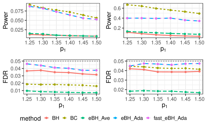
Figure 1: FDR and power for Setting S1. The left panel and the right panel correspond to the cases of $n_{a}=100$ and $n_{a}=200$, respectively. The results are based on $500$ Monte Carlo replications.

In Setting S2. we set $n_{a}$ to be $50$ and 100, corresponding to $5\%$ and $10\%$ of all hypotheses. Under the null hypothesis, we generate the test statistics $X_{i}$ from the standard normal distribution $\mathcal{N}(0,1)$. Under the alternatives, $X_{i}$ follows $\mathcal{N}(\mu\log(n),1)$, where the parameter $\mu$ controls the signal strength, which varies between $0.3$ and $0.5$. Subsequently, the p-values are computed as $p_{i}=1-\Phi(X_{i})$, where $\Phi$ denotes the distribution function of the standard normal distribution. The simulation results are presented in Figure 2. When the signal density is 5% (i.e., $n_{a}=50$), the BH procedure performs better than the BC procedure. eBH_Ada has nearly the same power as the BH procedure, and it again outperforms eBH_Ave, which slightly improves over the BC procedure. When the signal density increases to 10% (i.e., $n_{a}=100$), the performance gap between the BH and BC procedures diminishes. eBH_Ada and its fast version produce almost the same power as the BH procedure, outperforming both the eBH_Ave and BC procedures. In this case, the performance of eBH_Ave is worse than that of the BH and BC procedures.

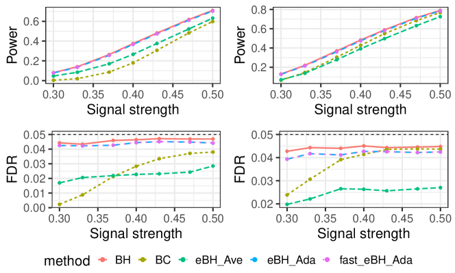
Figure 2: FDR and power for Setting S2. The left panel and the right panel correspond to the cases of $n_{a}=50$ and $n_{a}=200$, respectively. Results are based on $500$ Monte Carlo replications.

In summary, eBH_Ada is capable of improving the worse-performing method within the BH and BC procedures under different scenarios. Interestingly, its power can be nearly identical to the better-performing method, which demonstrates the adaptivity of eBH_Ada. fast_eBH_Ada delivers almost the same results as eBH_Ada in all settings with a much lower computational burden. We therefore recommend the use of fast_eBH_Ada in practice.

4.2 Fair multiple testing

In recent years, there has been a growing interest in developing machine learning algorithms that ensure certain notion of fairness for groups categorized by protected attributes, such as gender, race, or ethnicity. However, the development of statistical inference procedures that guarantee specific notions of fairness has not received the same level of attention. To address this gap, we introduce a new notion of fairness in the context of multiple hypothesis testing, and propose a procedure to ensure this notion of fairness.

Suppose we have $n$ hypotheses which can be partitioned into $G$ distinct groups, denoted as $\{\mathcal{G}_{g}\colon g=1,\dots,G\}$, according to some protected attributes, where $\cup_{g=1}^{G}\mathcal{G}_{g}=[n]:=\{1,2,\dots,n\}$ and $\mathcal{G}_{g}\cap\mathcal{G}_{g^{\prime}}=\emptyset$ for $g\neq g^{\prime}$. Recall that $\theta_{i}\in\{0,1\}$ represents the underlying truth of $H_{i}$ and $\delta_{i}\in\{0,1\}$ denotes the decision rule for $H_{i}$. We define the group-wise FDP and FDR based on $\bm{\delta}$ respectively as:

$$\mathrm{FDP}_{g}(\bm{\delta})=\frac{\sum_{i\in\mathcal{G}_{g}}(1-\theta_{i})\delta_{i}}{1\vee\sum_{i\in\mathcal{G}_{g}}\delta_{i}},\quad\text{FDR}_{g}(\bm{\delta})=\mathbb{E}[\text{FDP}_{g}(\bm{\delta})],\quad g=1,2,\dots,G.$$

Definition 1.

A decision rule $\bm{\delta}$ with the target FDR level $\alpha$ is called a fair decision rule if it controls both the group-wise FDRs uniformly over $1\leq g\leq G$ and the overall FDR at the level $\alpha$, i.e., $\max_{1\leq g\leq G}\text{FDR}_{g}(\bm{\delta})\leq\alpha$ and $\text{FDR}(\bm{\delta})\leq\alpha$.

Remark 1.

Among various notions of fairness that have been discussed in the literature (Verma and Rubin, 2018), predictive parity in the classification context (Chouldechova, 2017) is most relevant to our definition of fairness. To elaborate, let us consider a binary classification problem where $Y\in\{0,1\}$ represents the true labels and $\widehat{Y}\in\{0,1\}$ denotes the predicted labels. In this scenario, the FDR is defined as $P(Y=0|\widehat{Y}=1)$. A classifier satisfies predictive parity if it ensures an equal FDR across all groups. However, the multiple testing problem differs from the classification problem as the underlying truth of each hypothesis is unobserved and cannot be used to construct the decision rule. In our context, it is more appropriate to control the FDRs across different groups at the same desired level rather than forcing them to be the same.

We illustrate our definition of a fair decision rule through a makeup example below. Imagine a scenario where a parole commission uses machine learning algorithms to decide whether to grant a prisoner parole, and the prisoners are partitioned into two groups based on their race (i.e., white and black). Let $\theta_{i}=0$ ($\theta_{i}=1$) if the $i$th prisoner has a high (low) risk of recommitting a crime if granted parole. Set $\delta_{i}=1$ ($\delta_{i}=0$) if the machine learning algorithm decides to (not to) release the $i$th prisoner. To ensure that the decision rule associated with the machine learning algorithm controls the potential risk of the prisoners who are granted parole to society, we aim to control the FDR. Specifically, we want to ensure that the overall FDR is controlled at a pre-specified level while also ensuring that the algorithm is fair to both race groups by requiring the FDR for each group to be controlled at the same level. Assuming that there are two candidate machine learning algorithms under consideration by the parole commission, we refer to them as Algorithms A and B. Algorithm A is designed to control the overall FDR (e.g., by applying the BH or BC procedure to all prisoners, regardless of their race information). Algorithm B, on the other hand, ensures FDR control for individual groups by applying the same procedure separately to each group. We argue that neither Algorithm A nor B is desirable, as they may fail to control either the group FDR (for Algorithm A) or the overall FDR (for Algorithm B). For instance, in our simulation setting E2 in Section 4.2.2, Algorithm A fails to control the FDR for the second group, while Algorithm B fails to control the overall FDR. To illustrate these FDR outcomes, we have included Table 1, which displays the overall FDR (FDR${}_{\text{overall}}$) and the FDR for the two separate groups (FDR₁ and FDR₂) with a targeted FDR level of $0.05$.

Algorithm	FDR${}_{\text{overall}}$	FDR1	FDR2
Algorithm A	0.039	0.006	0.067
Algorithm B	0.057	0.048	0.025

Table 1: FDR results for Setting E2, where the nominal FDR level is $5\%$.

To overcome the issues above, we consider a multiple testing procedure by assembling the e-values from the BC procedure applied to each group separately. Specifically, we implement the BC procedure at the level $\alpha$ for each individual group and let

$$T_{g}=\sup\left\{0<t<0.5\colon\frac{1+\sum_{i\in\mathcal{G}_{g}}\mathbbm{1}\{p_{i}\geq 1-t\}}{1\vee\sum_{i\in\mathcal{G}_{g}}\mathbbm{1}\{p_{i}\leq t\}}\leq\alpha\right\}$$ (15)

be the rejection threshold for the $g$th group with $1\leq g\leq G$. Define

$$e_{i}=\frac{n_{g}w_{i}\mathbbm{1}\{p_{i}\leq T_{g}\}}{1+\sum_{j\in\mathcal{G}_{g}}\mathbbm{1}\{p_{j}\geq 1-T_{g}\}},$$ (16)

for $i\in\mathcal{G}_{g}$, where $w_{i}>0$ represents the weight for the $i$th hypothesis, which will be specified in Section 4.2.1. After collecting the e-values from each group, we implement the e-BH procedure at level $\alpha$. The testing procedure is summarized in Algorithm 2.

Algorithm 2 Fair multiple testing

p-values $p_{1},\dots,p_{n}$, group indices $\mathcal{G}_{1},\dots,\mathcal{G}_{G}$, significance level $\alpha$

for $g=1,\dots,G$ do

     Implement the BC procedure utilizing the p-values $\{p_{i}\colon i\in\mathcal{G}_{g}\}$ at the level $\alpha$.

     Calculate the threshold $T_{g}$ using (15).

     for $i\in\mathcal{G}_{g}$ do

         Calculate the e-value $e_{i}$ using (16).

     end for

end for

Assemble the e-values from all groups.

Run the e-BH procedure utilizing the assembled e-values at the level $\alpha$.

The indices of rejected hypotheses.

It is important to note that only the nonzero e-values can be rejected in the e-BH procedure. As a result, the group-wise FDR is effectively controlled at level $\alpha$ for each group. In the following section, we will demonstrate that the e-BH procedure can effectively control the overall FDR even when the weights are selected in a data-dependent manner.

4.2.1 Choice of weights and FDR control

Controlling the overall FDR requires ensuring that the e-values defined in (16) satisfy Condition (3). One strategy is to set $w_{i}=1$ for all $i$. Another strategy takes into account the group size by setting $w_{i}=n/(Gn_{g})$ for all $i\in\mathcal{G}_{g}$ and $g=1,\dots,G$, where $n_{g}=|\mathcal{G}_{g}|$ is the cardinality of the $g$th group. It can be verified that Condition (3) is satisfied by both strategies. The e-BH procedures based on these two weight choices are referred to as eBH_1 and eBH_2, respectively.

Theorem 6.

Suppose that the null p-values $\{p_{i}\}_{i\in\mathcal{H}_{0}}$ are mutually independent and satisfy Condition (8), and are independent of the alternative p-values $\{p_{i}\}_{i\notin\mathcal{H}_{0}}$. Further suppose the weights $w_{i}$ are independent of the p-values and satisfy

$$\sum_{g=1}^{G}n_{g}\max_{i\in\mathcal{G}_{g}}w_{i}\leq n.$$ (17)

Then, the e-values specified in (16) satisfy Condition (3). Hence, the corresponding e-BH procedure controls the FDR in finite sample.

Our simulations show that eBH_1 and eBH_2 frequently suffer from low statistical power. To enhance efficiency, we suggest utilizing a data-dependent weight selection approach inspired by the leave-one-out technique (Barber et al., 2020).

Denote the p-values in the $g$th group by $\mathbf{p}_{g}=\{p_{i}\}_{i\in\mathcal{G}_{g}}$. Write $\tilde{p}_{i}=\min\{p_{i},1-p_{i}\}$, and let $\mathbf{p}_{g,i}$ for $i\in\mathcal{G}_{g}$ be the collection of p-values obtained by replacing $p_{i}$ with $\tilde{p}_{i}$ in $\mathbf{p}_{g}$. By viewing $T_{g}$ as a functions of $\mathbf{p}_{g}$, we define $T_{g,i}=T_{g}(\mathbf{p}_{g,i})$, i.e., the threshold of the BC procedure applied to the set of p-values $\mathbf{p}_{g,i}$. We define the data-dependent weights as

$$w_{i}=\frac{\frac{n}{n_{g}}\left(1+\sum_{j\neq i,j\in\mathcal{G}_{g}}\mathbbm{1}\{p_{j}\geq 1-T_{g}\}\right)}{\left(1+\sum_{j\neq i,j\in\mathcal{G}_{g}}\mathbbm{1}\{p_{j}\geq 1-T_{g}\}\right)+\sum_{g^{\prime}\neq g}\sum_{j\in\mathcal{G}_{g^{\prime}}}\mathbbm{1}\{p_{j}\geq 1-T_{g^{\prime},j}\}},$$ (18)

for $i\in\mathcal{G}_{g}$. When $G=2$, we have

$$w_{i}=\frac{\frac{n}{n_{1}}\left(1+\sum_{j\neq i,j\in\mathcal{G}_{1}}\mathbbm{1}\{p_{j}\geq 1-T_{1}\}\right)}{\left(1+\sum_{j\neq i,j\in\mathcal{G}_{1}}\mathbbm{1}\{p_{j}\geq 1-T_{1}\}\right)+\sum_{j\in\mathcal{G}_{2}}\mathbbm{1}\{p_{j}\geq 1-T_{2,j}\}}$$

for $i\in\mathcal{G}_{1}$ and

$$w_{i}=\frac{\frac{n}{n_{2}}\left(1+\sum_{j\neq i,j\in\mathcal{G}_{2}}\mathbbm{1}\{p_{j}\geq 1-T_{2}\}\right)}{\sum_{j\in\mathcal{G}_{1}}\mathbbm{1}\{p_{j}\geq 1-T_{1,j}\}+\left(1+\sum_{j\neq i,j\in\mathcal{G}_{2}}\mathbbm{1}\{p_{j}\geq 1-T_{2}\}\right)}$$

for $i\in\mathcal{G}_{2}$. The e-BH procedure based on the weights specified in (18) is referred to as the eBH_Ada method in the following discussions. The theorem below states that eBH_Ada has finite sample FDR control.

Theorem 7.

Suppose that the null p-values $\{p_{i}\}_{i\in\mathcal{H}_{0}}$ are mutually independent and satisfy Condition (8), and are independent of the alternative p-values $\{p_{i}\}_{i\notin\mathcal{H}_{0}}$. Then, the e-values specified in (16) with the weights defined via (18) satisfy Condition (3). Hence, the corresponding e-BH procedure controls the FDR in finite sample.

4.2.2 Numerical studies

We shall compare the finite sample performance of the proposed method with two naive approaches through simulations. The first method disregards the group information and directly applies the BC procedure to all p-values. We refer to this method as BC_Com for future reference. BC_Com has two shortcomings. Firstly, it may fail to control the group-wise FDRs, as illustrated in Setting E2. Secondly, it fails to ensure comparable power across different groups, resulting in the possibility of one group having high power while the other group has nearly zero power, as illustrated in Setting E1. The same issue is also encountered by eBH_1. An alternative approach involves implementing the BC procedure for each group separately and combining all rejections. We call this method BC_Sep. Although BC_Sep effectively controls the FDR for individual groups, it does not guarantee the overall FDR control.

Remark 2.

We also tried BC_Sep at the level $\alpha/G$, a naive method that controls both the group-wise and overall FDRs. Indeed, let $\hat{n}_{ga}$ be the number of rejections for the $g$th group, and denote the number of false rejections for the $g$th group by $\hat{n}_{g0}$. Then we have $\mathbb{E}[\hat{n}_{g0}/(1\vee\hat{n}_{ga})]\leq\alpha/G$, which implies that

$$\mathbb{E}\left[\frac{\sum_{g=1}^{G}\hat{n}_{g0}}{1\vee\sum_{g=1}^{G}\hat{n}_{ga}}\right]\leq\mathbb{E}\left[\sum_{g=1}^{G}\frac{\hat{n}_{g0}}{1\vee\hat{n}_{ga}}\right]\leq\alpha.$$

However, this method has nearly zero power in all our simulation settings. Therefore, we have decided not to include its results in the tables below.

We first consider the case of two groups. To evaluate each method, we employ the following metrics: POW represents the overall power combining the rejections from both groups; POW₁ denotes the power for the first group, while POW₂ represents the power for the second group. Similarly, we can define FDR, FDR₁, and FDR₂. The empirical power and FDR are computed based on 1,000 independent Monte Carlo simulations.

In all settings, we assume that the p-values follow the uniform distribution on $[0,1]$ under the null. For the first group, the p-value is assumed to follow $\mathrm{Unif}[0,u_{1}]$ under the alternatives, while for the second group, it follows $\mathrm{Unif}[0,u_{2}]$ under the alternatives. The parameter values for different settings are detailed in Table 2.

Setting	$n_{1}$	$n_{1a}$	$u_{1}$	$n_{2}$	$n_{2a}$	$u_{2}$
E1	$100$	$20$	$1.5\times 10^{-2}$	$1000$	$20$	$1.5\times 10^{-3}$
E2	$100$	$20$	$1.5\times 10^{-3}$	$1000$	$20$	$1.5\times 10^{-3}$

Table 2: Parameter settings for the case of $G=2$. Here, $n_{g}$ represents the number of hypotheses for the $g$th group; $n_{ga}$ denotes the number of non-null hypotheses in the $g$th group. The parameter $u_{g}$ is the upper bound of the uniform distribution for the p-values under the alternatives for the $g$th group.

Setting E1 corresponds to a scenario in which, for instance, the first group consists of ethnic minorities while the second group comprises of majorities. The number of non-nulls are the same across the two groups. The alternative p-values in the first group are larger than those in the second group on average as $u_{1}>u_{2}$. Table 3 summarizes the results for this setting. BC_Com exhibits high power for the second group, yet its power in the first group are rather low. This is because the non-null p-values from the first group are not sufficiently small, and a combined analysis of the two groups demands a lower threshold and thus fails to reject them. Additionally, BC_Sep has a slightly inflated overall FDR in this case.

Method	POW	POW1	POW2	FDR	FDR1	FDR2
BC_Com	0.144	0.041	0.248	0.023	0.012	0.025
BC_Sep	0.296	0.352	0.24	0.053	0.036	0.025
eBH_1	0.07	0	0.141	0.02	0	0.02
eBH_2	0.078	0.077	0.078	0.008	0.008	0.008
eBH_Ada	0.181	0.212	0.149	0.028	0.021	0.015

Table 3: FDR and power for Setting E1, where the nominal FDR level is 5%.

Setting E2 is the same as Setting E1 except that $u_{1}=u_{2}=1.5\times 10^{-2}$. The results for Setting E2 are presented in Table 4. We observe that BC_Com fails to control the FDR for the second group, which can be explained as follows. Due to the fact that the non-null p-values have a similar scale for both groups and the sample size of the first group is significantly smaller than that of the second group, BC_Com has a higher threshold compared to the BC procedure applied only to the second group. This can result in an FDR inflation in the second group for BC_Com. We also observe that BC_Sep suffers from an overall FDR inflation. In contrast, all three variants of the e-BH procedure control the group-wise and overall FDRs at the desired level. eBH_Ada has a much higher power than the other two e-value based methods.

Method	POW	POW1	POW2	FDR	FDR1	FDR2
BC_Com	0.605	0.605	0.606	0.039	0.006	0.067
BC_Sep	0.573	0.906	0.24	0.057	0.048	0.025
eBH_1	0.07	0	0.141	0.02	0	0.02
eBH_2	0.216	0.217	0.215	0.017	0.011	0.022
eBH_Ada	0.384	0.552	0.216	0.036	0.029	0.023

Table 4: FDR and power for Setting E2, where the nominal FDR level is 5%.

We present the results for $G=4$ in Appendix C.1, where we consider three different scenarios (Settings F1-F3). In particular, we note that BC_Com suffers from a severe FDR inflation with the empirical FDR being 0.312 at the 5% target level in Setting F2. In Setting F3, BC_Sep has an empirical overall FDR being 0.346, which is much higher than the 20% level.

To summarize, as seen in Settings E2 and F2, BC_Com has no guarantee in controlling the group-wise FDR. On the other hand, BC_Sep fails to control the overall FDR, as observed in all the settings, particularly Settings E2 and F3 in Appendix C.1. The e-BH based approaches provide both group-wise and overall FDR control, making them fair according to Definition 1. However, eBH_1 and eBH_2 may suffer from power loss under certain scenarios. In contrast, eBH_Ada demonstrates consistent effectiveness across all settings by achieving FDR fairness and reasonable power.

4.3 Structure adaptive multiple testing

Having access to various types of auxiliary information that reflect the structural relationships among hypotheses is becoming increasingly common. Taking advantage of such auxiliary information can improve the statistical power in multiple testing. In this section, we consider the scenarios where, in addition to the p-value $p_{i}$, there is associated structural information in the form of a covariate $x_{i}$ for each hypothesis. This side information represents heterogeneity among the p-values and may affect the prior probabilities of the null hypotheses being true or the signal strength under alternatives. Our goal is to develop a multiple testing procedure that can incorporate such external structural information to improve statistical power and has guaranteed FDR control in finite sample. The high-level idea behind our approach is to relax the p-value thresholds for hypotheses that are more likely to be non-null and tighten the thresholds for the other hypotheses through the use of hypothesis-specific rejection rule, i.e., $\varphi_{i}(p_{i})\leq t$, so that the FDR can be controlled.

Our proposed method combines the cross-fitting technique (Ignatiadis and Huber, 2021) (a sample-splitting and fitting approach that enables learning the hypothesis-specific rejection function $\varphi_{i}$ without overfitting as long as the hypotheses can be partitioned into independent folds) with the GBC procedure introduced in Section 3. First, we randomly split the data into $G$ distinct groups, denoted as $\{\mathcal{G}_{g}\colon g=1,\dots,G\}$, where $\bigcup_{g=1}^{G}\mathcal{G}_{g}=[n]$ and $\mathcal{G}_{g}\cap\mathcal{G}_{g^{\prime}}=\emptyset$ for $g\neq g^{\prime}$. We estimate the rejection function $\varphi_{i}$ for the hypothesis $i$ in the $g$th group using the data from all other groups, which ensures that the estimated rejection function is independent of the p-values in group $g$. We then apply the GBC procedure based on the estimated rejection functions separately to each group and obtain the corresponding e-values. Finally, we collect all the e-values and apply the e-BH procedure at the target level to control the FDR.

To describe the cross-fitting procedure, let us assume that $\varphi_{i}(p)=\varphi(p,x_{i};\beta)$ for some unknown parameter $\beta$ that needs to be estimated from the data. We define the cross-fitted estimate as

$$\hat{\beta}_{-g}=\operatorname*{arg\,min}_{\beta}\sum_{i\notin\mathcal{G}_{g}}\mathcal{L}(p_{i},x_{i},\beta).$$

Here $\mathcal{L}$ is some loss function such as negative log-likelihood under the two-group mixture model in Example 3, in which case we assume $\pi_{i}(p)=\pi(p,x_{i};\beta_{1})$, $f_{1,i}(p)=f(p,x_{i};\beta_{2})$ and $\beta=(\beta_{1},\beta_{2}).$ It should be noted that the choice of the functional form of $\varphi_{i}$ is highly flexible and does not impact the FDR control due to cross-fitting that avoids over-fitting. Given $\hat{\beta}_{-g}$, we define

$$\hat{\varphi}_{i}(p)=\varphi(p,x_{i};\hat{\beta}_{-g})\quad\text{for}\quad i\in\mathcal{G}_{g}.$$

Next, we apply the GBC procedure using the cross-fitted functions $\{\hat{\varphi}_{i}(\cdot)\}_{i\in\mathcal{G}_{g}}$ at the level $\alpha_{\mathrm{GBC}}$. The corresponding threshold for the $g$th group is given by

$$T_{g}=\sup\left\{0<t\leq T_{g,\mathrm{up}}\colon\frac{1+\sum_{i\in\mathcal{G}_{g}}\mathbbm{1}\{\hat{\varphi}_{i}(1-p_{i})\leq t\}}{1\vee\sum_{i\in\mathcal{G}_{g}}\mathbbm{1}\{\hat{\varphi}_{i}(p_{i})\leq t\}}\leq\alpha_{\mathrm{GBC}}\right\},$$ (19)

where $T_{g,\mathrm{up}}$ satisfies $T_{g,\mathrm{up}}<\min_{i\in\mathcal{G}_{g}}\hat{\varphi}_{i}(0.5)$. We define the e-value for all $i\in\mathcal{G}_{g}$ as

$$e_{i}=\frac{n_{g}w_{i}\mathbbm{1}\{\hat{\varphi}_{i}(p_{i})\leq T_{g}\}}{1+\sum_{j\in\mathcal{G}_{g}}\mathbbm{1}\{\hat{\varphi}_{j}(1-p_{j})\leq T_{g}\}},$$ (20)

where $w_{i}>0$ represents the e-value weight for hypothesis $i$ in group $G_{g}$. Finally, we aggregate all e-values from each group and implement the e-BH procedure. A detailed description of our procedure is given in Algorithm 3.

Algorithm 3 Cross-fitting based structure adaptive multiple testing

p-values $p_{1},\dots,p_{n}$, covariates $x_{1},\dots,x_{n}$, group indices $\mathcal{G}_{1},\dots,\mathcal{G}_{G}$, significance levels $\alpha_{\mathrm{GBC}}$ and $\alpha_{\mathrm{eBH}}$

for $g=1,\dots,G$ do

     Compute the estimate of the rejection rule $\hat{\varphi}_{i}(\cdot)$ for $i\in\mathcal{G}_{g}$ using $\mathbf{p}_{-g}$ and $\mathbf{x}_{-g}$.

     Calculate the threshold $T_{g}$ using (19).

     for $i\in\mathcal{G}_{g}$ do

         Calculate the e-value $e_{i}$ using (20).

     end for

end for

Assemble the e-values from all groups.

Run the e-BH procedure utilizing the assembled e-values at the level $\alpha_{\mathrm{eBH}}$.

The indices of rejected hypotheses.

4.3.1 Choice of weights and FDR control

To ensure that the FDR is controlled at the desired level, it is crucial to verify that the e-values defined in equation (20) satisfy Condition (3). We shall show that under certain conditions on the weights, the e-values defined by (20) satisfy (3), and as a result, the corresponding e-BH procedure controls the FDR at the desired level. Before stating the main theorem, let us first introduce some notation. Define $\tilde{p}_{i}=\min\{p_{i},1-p_{i}\}$, $\mathbf{p}_{g}=\{p_{i}\}_{i\in\mathcal{G}_{g}}$, and $\mathbf{p}_{g,i}$ as the collection of p-values obtained by replacing $p_{i}$ with $\tilde{p}_{i}$ in $\mathbf{p}_{g}$ for $i\in\mathcal{G}_{g}$. Also, let $\mathbf{p}_{-g}=\{p_{i}\}_{i=1}^{n}\setminus\mathbf{p}_{g}$. Due to cross-fitting, the estimated function $\hat{\varphi}_{i}(\cdot)$ for $i\in\mathcal{G}_{g}$ only depends on $\mathbf{p}_{-g}$. Moreover, given the fitted functions $\hat{\varphi}_{i}$ for $i\in\mathcal{G}_{g}$, the threshold $T_{g}$ defined in (19) can be treated as a function of $\mathbf{p}_{g}$. Let $T_{g,j}=T_{g}(\mathbf{p}_{g,j};\{\hat{\varphi}_{l}\}_{l\in\mathcal{G}_{g}})$. We impose the following assumptions.

Assumption 1.

Let $\{(p_{i},x_{i})\}$ for $1\leq i\leq n$ be the p-value and covariate pairs.

1. The null pairs $\{(p_{i},x_{i})\}_{i\in\mathcal{H}_{0}}$ are mutually independent.

2. The null pairs $\{(p_{i},x_{i})\}_{i\in\mathcal{H}_{0}}$ are independent of the alternative pairs $\{(p_{i},x_{i})\}_{i\notin\mathcal{H}_{0}}$.

3. For $i\in\mathcal{H}_{0}$, $p_{i}$ is independent of $x_{i}$ and satisfies Condition (8).

Assumption 2.

For all $1\leq i\leq n$, $\varphi_{i}(\cdot,x_{i};\beta)$ is a monotonic increasing and continuous function given any $\beta$ and $x_{i}$.

Assumption 1 concerns the dependence of the null pairs, which is standard in the literature; see, e.g., Assumption 1 of Ignatiadis and Huber (2021) and Zhao and Zhou (2023). Assumption 2 implies that $P(\varphi_{i}(p_{i},x_{i};\beta)\leq b)\leq P(\varphi_{i}(1-p_{i},x_{i};\beta)\leq b)$ for all $\varphi_{i}(0,x_{i};\beta)\leq b\leq\varphi_{i}(0.5,x_{i};\beta)$, which will be used in our proof. We describe a concrete choice of $\varphi_{i}$ in Section 4.3.2 below.

Theorem 8.

Suppose Assumptions 1 and 2 hold. If the weights $\{w_{i}\}$ are independent of the p-values and covariate information and satisfy (17), then the e-values defined in (20) fulfills Condition (3).

A naive choice is to set $w_{i}=1$ for all $i=1,2,\cdots,n$, which satisfy (17). However, this choice of weights often leads to low statistical power in simulations. To improve efficiency, we propose a data-dependent approach for constructing the weights. Given the group index $g$, for $g^{\prime}\neq g$, $i\in\mathcal{G}_{g}$ and $j\in\mathcal{G}_{g^{\prime}}$, let $\hat{\varphi}_{j}^{g,i,p}$ be the cross-fitted function obtained by replacing $\mathbf{p}_{g}$ with $\mathbf{p}_{g,i}(p)$, where $\mathbf{p}_{g,i}(p)$ is the collection of p-values with $p_{i}$ replaced by $p$. Define $T_{g^{\prime},j}^{g,i,p}=T_{g^{\prime}}(\mathbf{p}_{g^{\prime},j};\{\hat{\varphi}_{l}^{g,i,p}\}_{l\in\mathcal{G}_{g^{\prime}}})$. For $i\in\mathcal{G}_{g}$ with $1\leq g\leq G$, we propose the following e-value weights:

$$w_{i}=\frac{\frac{n}{n_{g}}\left(1+\sum_{j\neq i,j\in\mathcal{G}_{g}}\mathbbm{1}\{\hat{\varphi}_{j}(1-p_{j})\leq T_{g}\}\right)}{\left(1+\sum_{j\neq i,j\in\mathcal{G}_{g}}\mathbbm{1}\{\hat{\varphi}_{j}(1-p_{j})\leq T_{g}\}\right)+\sup_{p\in[0,1]}\sum_{g^{\prime}\neq g}\sum_{j\in\mathcal{G}_{g^{\prime}}}\mathbbm{1}\{\hat{\varphi}_{j}^{g,i,p}(1-p_{j})\leq T_{g^{\prime},j}^{g,i,p}\}}.$$ (21)

In the case of $G=2$, we have

$$w_{i}=\frac{\frac{n}{n_{1}}\left(1+\sum_{j\neq i,j\in\mathcal{G}_{1}}\mathbbm{1}\{\hat{\varphi}_{j}(1-p_{j})\leq T_{1}\}\right)}{\left(1+\sum_{j\neq i,j\in\mathcal{G}_{1}}\mathbbm{1}\{\hat{\varphi}_{j}(1-p_{j})\leq T_{1}\}\right)+\sup_{p\in[0,1]}\sum_{j\in\mathcal{G}_{2}}\mathbbm{1}\{\hat{\varphi}_{j}^{1,i,p}(1-p_{j})\leq T_{2,j}^{1,i,p}\}}$$

for $i\in\mathcal{G}_{1}$ and

$$w_{i}=\frac{\frac{n}{n_{2}}\left(1+\sum_{j\neq i,j\in\mathcal{G}_{2}}\mathbbm{1}\{\hat{\varphi}_{j}(1-p_{j})\leq T_{2}\}\right)}{\sup_{p\in[0,1]}\sum_{j\in\mathcal{G}_{1}}\mathbbm{1}\{\hat{\varphi}_{j}^{2,i,p}(1-p_{j})\leq T_{1,j}^{2,i,p}\}+\left(1+\sum_{j\neq i,j\in\mathcal{G}_{2}}\mathbbm{1}\{\hat{\varphi}_{j}(1-p_{j})\leq T_{2}\}\right)}$$

for $i\in\mathcal{G}_{2}$. The construction of $w_{i}$ involves taking supremum over $p$, which is crucial for the proof to go through. On the one hand, it renders $w_{i}$ independent of $p_{i}$, which is a useful fact in the proof. On the other hand, it makes the weight sufficiently small in the sense that we can upper bound $w_{i}$ with the term $\sup_{p\in[0,1]}\sum_{j\in\mathcal{G}_{1}}\mathbbm{1}\{\hat{\varphi}_{j}^{2,i,p}(1-p_{j})\leq T_{1,j}^{2,i,p}\}$ in its denominator replaced by $\sum_{j\in\mathcal{G}_{1}}\mathbbm{1}\{\hat{\varphi}_{j}(1-p_{j})\leq T_{1,j}\}$, which is another fact used in our argument.

Theorem 9.

Suppose Assumptions 1 and 2 hold. Then, the e-values defined in (20) with weights specified by (21) satisfy Condition (3).

4.3.2 Simulation studies

We shall compare the finite sample performance of the proposed method with several existing approaches through simulation studies. Throughout, we fix the sample size $n=3,000$ and set the target FDR level at $\alpha_{\mathrm{eBH}}=0.1$. For each experimental setting, we conduct 100 simulations, and report the average FDP (as an estimate of the FDR) and power over the independent simulation runs.

We begin by providing the implementation details of the proposed method. In the GBC procedure, we utilize the rejection rule based on the local FDR under the two group mixture model in Example 3, where we set $f_{0}(p)=\mathbbm{1}\{p\in[0,1]\}$ and $f_{1,i}(p)=(1-\pi_{i})(1-\kappa_{i})p^{-\kappa_{i}}$ with $\kappa_{i}\in(0,1).$ We consider the working models that link $(\pi_{i},\kappa_{i})$ with the external covariates:

$$\pi_{i} =\pi_{\beta_{\pi}}(x_{i})=\frac{1}{1+\exp(-\beta_{\pi,0}-\beta_{\pi,1}^{\top}x_{i})},$$

$$\kappa_{i} =\kappa_{\beta_{\kappa}}(x_{i})=\frac{1}{1+\exp(-\beta_{\kappa,0}-\beta_{\kappa,1}^{\top}x_{i})},$$

where the parameters $\beta_{\pi}=(\beta_{\pi,0},\beta_{\pi,1}^{\top})\in\mathbb{R}^{d+1}$ and $\beta_{\kappa}=(\beta_{\kappa,0},\beta_{\kappa,1}^{\top})\in\mathbb{R}^{d+1}$ can be estimated by maximizing the pseudo-log-likelihood using the EM algorithm. Please refer to Zhang and Chen (2022) for more optimization details. After obtaining the estimates $\hat{\beta}_{\pi}$ and $\hat{\beta}_{\kappa}$ from the EM algorithm, we define

$$\hat{\pi}_{i}=\begin{cases}\epsilon_{1}&\text{if }1/\bigl{(}1+\exp(-\hat{\beta}_{\pi,0}-\hat{\beta}_{\pi,1}^{\top}x_{i})\bigr{)}\leq\epsilon_{1},\\ 1/\bigl{(}1+\exp(-\hat{\beta}_{\pi,0}-\hat{\beta}_{\pi,1}^{\top}x_{i})\bigr{)}&\text{if }\epsilon_{1}<1/\bigl{(}1+\exp(-\hat{\beta}_{\pi,0}-\hat{\beta}_{\pi,1}^{\top}x_{i})\bigr{)}<1-\epsilon_{2},\\ 1-\epsilon_{2}&\text{otherwise,}\end{cases}$$

where winsorization is used to prevent $\hat{\pi}_{i}$ from being too close to zero or one to stabilize the algorithm. We define the rejection rule

$$\hat{\varphi}_{i}(p)=\frac{1}{\hat{\pi}_{i}+(1-\hat{\pi}_{i})(1-\hat{\kappa}_{i})p^{-\hat{\kappa}_{i}}}\leq t,$$

where $\hat{\kappa}_{i}=1/\bigl{(}1+\exp(-\beta_{\kappa,0}-\hat{\beta}_{\kappa,1}^{\top}x_{i})\bigr{)}$. Additionally, to speed up the procedure, we propose the following weight that is computationally less expensive:

$$w_{i}=\frac{\frac{n}{n_{g}}\left(1+\sum_{j\neq i,j\in\mathcal{G}_{g}}\mathbbm{1}\{\hat{\varphi}_{j}(1-p_{j})\leq T_{g}\}\right)}{\left(1+\sum_{j\neq i,j\in\mathcal{G}_{g}}\mathbbm{1}\{\hat{\varphi}_{j}(1-p_{j})\leq T_{g}\}\right)+\sum_{g^{\prime}\neq g}\sum_{j\in\mathcal{G}_{g^{\prime}}}\mathbbm{1}\{\hat{\varphi}_{j}(1-p_{j})\leq T_{g,j}\}}.$$

We fix $\epsilon_{1}=0.1$, $\epsilon_{2}=1\times 10^{-5}$, $G=2$, and $\alpha_{\mathrm{GBC}}=\alpha_{\mathrm{eBH}}/(1+\alpha_{\mathrm{eBH}})$. We refer to this method as eBH_GBC for future reference. We compare the proposed method with the following competing methods:

• BH: The BH procedure (Benjamini and Hochberg, 1995). We implement this method using the p.adjust function in R.

• IHW_storey: The covariate-powered cross-weighted method with the Storey’s procedure to estimate the null-proportion (Ignatiadis and Huber, 2021). We implement this method using the ihw_bh function in the R package IHWStatsPaper.

• IHW_betamix: The covariate-powered cross-weighted method with the beta mixture model (Ignatiadis and Huber, 2021). We implement this method using the ihw_betamix_censored function in the R package IHWStatsPaper.

• AdaPT: The adaptive p-value thresholding procedure (Lei and Fithian, 2018). We implement this method using the adapt_glm function in the R package adaptMT.

• SABHA: The structure adaptive BH procedure (Li and Barber, 2019). The code was downloaded from the link provided by the original paper.

To illustrate the effect of the covariate, we generate a single covariate $x_{i}$ from the standard normal distribution. Given the value of $x_{i}$, we define $\pi_{i}$ as

$$\pi_{i}=\frac{\exp(a_{0}+a_{1}x_{i})}{1+\exp(a_{0}+a_{1}x_{i})},$$

where $a_{0}$ and $a_{1}$ determine the baseline signal density and the informativeness of the covariate, respectively. The values of $a_{0}$ and $a_{1}$ are fixed for each simulated dataset. Specifically, we set $a_{0}$ to take on values from the set $\{3.5,1.5,1.5\}$, achieving signal densities of approximately $3\%$, $8\%$, and $18\%$, respectively, representing sparse, medium, and dense signals. Furthermore, we set $a_{1}$ to take on values from the set $\{1.5,2,2.5\}$, representing a less informative, moderately informative, and strongly informative covariate, respectively. The underlying truth $\theta_{i}$ is then simulated based on $\pi_{i}:\theta_{i}\sim\text{Bernoulli}(1-\pi_{i}).$ We next generate the covariate that affects the alternative function $f_{1,i}$. Specifically, we sample another covariate $x_{i}^{\prime}\sim\mathcal{N}(0,1)$ and define

$$\eta_{i}=\frac{2\exp(a_{f}x_{i}^{\prime})}{1+\exp(a_{f}x_{i}^{\prime})},$$

where we set $a_{f}\in\{0,0.5,1\}$ for no informativeness, less informativeness, and strong informativeness. Then, the z-scores are sampled from

$$z_{i}\sim\mathcal{N}(\eta_{i}\mu\theta_{i},1),$$

where $\mu$ denotes the signal strength with the values evenly distributed in the interval $[2.5,3.4]$. These $z$-scores are transformed into p-values using the one-sided formula $1-\Phi(z_{i})$. The p-values, along with the corresponding covariates $x_{i}$ and $x_{i}^{\prime}$, serve as the input for the structure adaptive multiple testing methods.

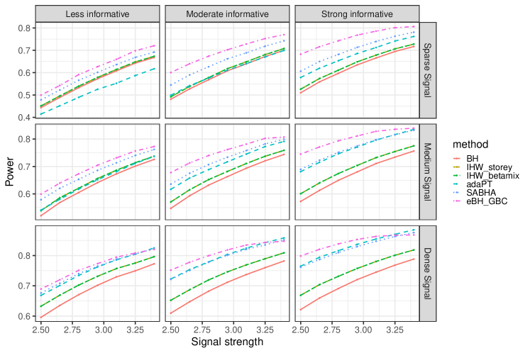
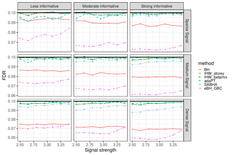
Figure 3: Empirical FDR and power for $a_{f}=1$.

Figure 3 shows the results for $a_{f}=1$. All methods successfully controlled the FDR at the desired level. When the signal is sparse ($a_{0}=3.5$), eBH_GBC is the most powerful method. The SABHA method has the second-best performance, while the two versions of IHW show only slight improvement over the BH procedure. When the covariate is less informative ($a_{1}=1.5$), AdaPT is less powerful than the BH procedure. As the covariate becomes strongly informative ($a_{1}=2.5$), all structure adaptive methods outperform the BH procedure in terms of power. Our proposed method exhibits the highest power in most cases, with only AdaPT surpassing eBH_GBC in power when the signal is dense ($a_{0}=1.5$) and the covariate is strongly informative ($a_{1}=2.5$). The results for the settings with $a_{f}=0$ and $a_{f}=0.5$ are deferred to Appendix C.2.

4.3.3 Real data examples

We analyzed three omics datasets: Airway (Himes et al., 2014), Bottomly (Bottomly et al., 2011), and MWAS (McDonald et al., 2018). The Airway and Bottomly datasets are transcriptomics data obtained from RNA-seq experiments, which have been analyzed previously by Ignatiadis et al. (2016); Lei and Fithian (2018); Zhang and Chen (2022). These two datasets are available in the airway and IHWStatsPaper packages, respectively. For both datasets, we used the logarithm of the “basemean” as the covariate and removed the samples with missing values, leaving us with 18,028 and 11,709 tests, respectively. We obtained the MWAS dataset from the publicly available data of the AmericanGut project (McDonald et al., 2018). We focused on a subset of subjects with ages greater than thirteen and with complete sex and country information. We excluded OTUs (clustered sequencing units representing bacterial species) observed in fewer than ten subjects, resulting in 3,394 OTUs tested using the Wilcoxon rank sum test on normalized abundances. We used the library size of samples as the external covariate.

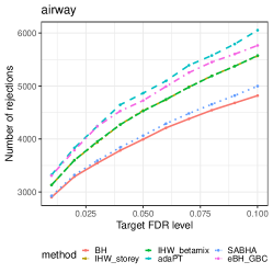
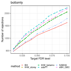
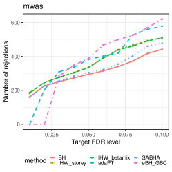
Figure 4: Number of discoveries of various methods with the target FDR level ranging from $0.01$ to $0.1$ in three real datasets.

The results of different methods for target FDR levels ranging from $0.01$ to $0.1$ are presented in Figure 4. AdaPT and eBH_GBC are the two methods that make the most discoveries (except for the MWAS data set with a target FDR level below 0.025). For the airway dataset, AdaPT consistently produces the most discoveries when the target FDR level is high. This is due to the high signal density of this data set. For instance, when the target FDR level is 10%, AdaPT is able to identify 6,053 discoveries out of 18,028 tests. It is worth noting that the proposed method performs similarly to AdaPT when the target FDR level is below 4%. We observe a similar phenomenon for the Bottomly dataset. For the MWAS dataset, AdaPT and eBH_GBC fail to make any discoveries when the target FDR level is 1%. This is a limitation of the BC-based method, which may have reduced power when the signal is very sparse. However, as the target FDR level increases, AdaPT and eBH_GBC quickly surpass the other methods in terms of the number of discoveries. eBH_GBC outperforms AdaPT with more discoveries when the FDR level is above 5%. Overall, eBH_GBC performs comparably to AdaPT.

5 Discussions

In this paper, we have shown that the BH and BC procedures, as well as their generalized versions, are all equivalent to the e-BH procedure based on some forms of e-values. This simple insight opens up new avenues for constructing multiple testing procedures in different contexts. Specifically, leveraging this idea, one can translate the testing results from different procedures or the same procedure for different subsets of the data into e-values. By aggregating or assembling these e-values, one can obtain a combined set of e-values that contains valuable information about various multiple testing procedures and subsets of the data. We have demonstrated the potential of this strategy in three applications, backed by rigorous theoretical analysis and numerical studies. An important aspect of our proposed methods is the use of data-dependent weights, which are constructed using the leave-one-out technique to aggregate and assemble e-values. Using these weights, we can obtain valid e-values that ensure the corresponding e-BH procedure controls the FDR in finite sample. The e-BH procedure based on the data-dependent weight is often more powerful than the unweighted version, but it comes at the cost of more expensive computation. Through simulations, we have demonstrated that a more cost-friendly version of these weights exists, which achieves nearly identical performance with a much lower computational burden.

We envision the idea of aggregating different multiple testing results through e-values to be useful in other contexts, such as meta-analysis or federated learning. Other interesting future research problems include finding the optimal way of combining the e-values with respect to certain criteria and investigating the robustness of the proposed methods when the data exhibit dependence.

Appendix

Appendix A Proof of the main results

We first state the following propositions whose proofs are deferred to Appendix  B. These results will be used frequently in the subsequent proofs of the main theorems.

Proposition 5 (Lemma 6 of Barber et al. [2020]).

Let $T_{\mathrm{BC},i}$ be the threshold for the BC methods when $p_{i}$ is replaced with $\min\{p_{i},1-p_{i}\}$. For any $i$, $j$, if $\min(p_{i},p_{j})\geq 1-\max\{T_{\mathrm{BC},i},T_{\mathrm{BC},j}\}$, then we have $T_{\mathrm{BC},i}=T_{\mathrm{BC},j}$.

Proposition 6.

Suppose the assumptions in Proposition 4 hold. Let $T_{i}$ be the threshold for the generalized BC methods when $p_{i}$ is replaced with $\min\{p_{i},1-p_{i}\}$. For any $i$, $j$, if $\max\{\varphi_{i}(1-p_{i}),\varphi_{j}(1-p_{j})\}\leq\max\{T_{i},T_{j}\}$, then we have $T_{i}=T_{j}$.

A.1 Proof of Theorem 1

Proof.

Theorem 1 is a special case of Theorem 2 by choosing $\varphi_{i}$ as the identity function for all $1\leq i\leq n$. ∎

A.2 Proof of Theorem 2

Proof.

Let $\hat{k}$ be the cardinality of $\mathcal{S}_{\mathrm{GBH}}$. If $i\notin\mathcal{S}_{\mathrm{GBH}}$, then $\varphi_{i}(p_{i})>T_{\mathrm{GBH}}$ and thus $e_{i}=0$. This implies that the $i$th hypothesis is not rejected by the e-BH procedure, and hence $\mathcal{S}_{\mathrm{eBH}}\subset\mathcal{S}_{\mathrm{GBH}}$. Conversely, if $i\in\mathcal{S}_{\mathrm{GBH}}$, we have $\varphi_{i}(p_{i})\leq T_{\mathrm{GBH}}\leq\bar{F}^{-1}\left(\frac{\alpha\hat{k}}{n}\right)$, leading to

$$e_{i}=\frac{1}{\bar{F}(T_{\mathrm{GBH}})}\geq\frac{n}{\alpha\hat{k}}$$

as $\bar{F}$ is strictly increasing. Define $e_{(i)}=n\mathbbm{1}\{q_{(i)}\leq T_{\mathrm{GBH}}\}/\sum_{j=1}^{n}F_{j}(T_{\mathrm{GBH}})$ for $1\leq i\leq n,$ where $q_{(1)}\leq\dots\leq q_{(n)}$ are the order statistics of $\{q_{i}=\varphi_{i}(p_{i})\}^{n}_{i=1}$. Let $\hat{k}$ represent the maximum $i$ for which $q_{(i)}\leq T_{\mathrm{GBH}}$. We get

$$e_{(\hat{k})}\geq\frac{n}{\alpha\hat{k}},$$ (A.1)

which indicates that $|\mathcal{S}_{\mathrm{eBH}}|\geq\hat{k}$. Because $\mathcal{S}_{\mathrm{eBH}}\subset\mathcal{S}_{\mathrm{GBH}}$, it is clear that $\mathcal{S}_{\mathrm{eBH}}=\mathcal{S}_{\mathrm{GBH}}$. ∎

A.3 Proof of Theorem 3

Let $\hat{k}$ be the cardinality of $\mathcal{S}_{\mathrm{GBC}}$. If $i\notin\mathcal{S}_{\mathrm{GBC}}$, then $\varphi_{i}(p_{i})>T_{\mathrm{GBC}}$ and thus $e_{i}=0$. Hence the $i$th hypothesis is not rejected by the e-BH procedure, which implies that $\mathcal{S}_{\mathrm{eBH}}\subset\mathcal{S}_{\mathrm{GBC}}$. For the other direction, note that if $i\in\mathcal{S}_{\mathrm{GBC}}$, then $\varphi_{i}(p_{i})\leq T_{\mathrm{GBC}}$ and $1+\sum_{j=1}^{n}\mathbbm{1}\{\varphi_{j}(1-p_{j})\leq T_{\mathrm{GBC}}\}\leq\hat{k}\alpha$. Hence, we have

$$e_{i}\geq\frac{n}{\hat{k}\alpha}.$$

We sort the e-values in descending order as $e_{(1)}\geq\dots\geq e_{(n)}$. It is clear that $e_{(\hat{k})}\geq n/(\hat{k}\alpha)$. Thus, $|\mathcal{S}_{\mathrm{eBH}}|\geq\hat{k}$, which implies that $\mathcal{S}_{\mathrm{eBH}}=\mathcal{S}_{\mathrm{GBC}}$.

A.4 Proof of Theorem 4

Proof.

Consider the BH procedure and observe that for a given number of rejections $R_{\mathrm{BH}}$, $T_{\mathrm{BH}}=T_{\mathrm{BH}}(R_{\mathrm{BH}})$ is a deterministic function of $R_{\mathrm{BH}}$. Let $R_{\mathrm{BH}}(p_{i}\rightarrow 0)$ be the number of rejections obtained by replacing the p-value $p_{i}$ with 0. Using the above fact and that the weights are independent of the p-values, we have

$$\sum_{i\in\mathcal{H}_{0}}\mathbb{E}[w_{\mathrm{BH},i}e_{\mathrm{BH},i}]= \sum_{i\in\mathcal{H}_{0}}w_{\mathrm{BH},i}\mathbb{E}\left[\frac{1}{T_{\mathrm{BH}}}\mathbbm{1}\{p_{i}\leq T_{\mathrm{BH}}\}\right]$$

$$= \sum_{i\in\mathcal{H}_{0}}w_{\mathrm{BH},i}\sum_{k=1}^{n}\mathbb{E}\left[\frac{1}{T_{\mathrm{BH}}(k)}\mathbbm{1}\{p_{i}\leq T_{\mathrm{BH}}(k),R_{\mathrm{BH}}(p_{i}\rightarrow 0)=k\}\right]$$

$$\leq \sum_{i\in\mathcal{H}_{0}}w_{\mathrm{BH},i}\sum_{k=1}^{n}\mathbb{E}[\mathbbm{1}\{R_{\mathrm{BH}}(p_{i}\rightarrow 0)=k\}]$$

$$= \sum_{i\in\mathcal{H}_{0}}w_{\mathrm{BH},i}.$$

For the BC procedure, denote $\tilde{p}_{i}\coloneqq\min\{p_{i},1-p_{i}\}$ and $\mathbf{p}_{-i}\coloneqq\{p_{1},\dots,p_{i-1},\,\tilde{p}_{i},\,p_{i+1},\dots,p_{n}\}$. By viewing $T_{\mathrm{BC}}$ as a function of the p-values, we define $T_{\mathrm{BC},i}=T_{\mathrm{BC}}(\mathbf{p}_{-i})$. Let $\mathcal{F}_{i}$ be the sigma algebra generated by $\mathbf{p}_{-i}$. Then, we have

$$\sum_{i\in\mathcal{H}_{0}}\mathbb{E}[w_{\mathrm{BC},i}e_{\mathrm{BC},i}]= \sum_{i\in\mathcal{H}_{0}}w_{\mathrm{BC},i}\mathbb{E}\left[\frac{n\mathbbm{1}\{p_{i}\leq T_{\mathrm{BC}}\}}{1+\sum_{j=1}^{n}\mathbbm{1}\{p_{j}\geq 1-T_{\mathrm{BC}}\}}\right]$$

$$= \sum_{i\in\mathcal{H}_{0}}w_{\mathrm{BC},i}\mathbb{E}\left[\frac{n\mathbbm{1}\{p_{i}\leq T_{\mathrm{BC},i}\}}{1+\sum_{j\neq i}\mathbbm{1}\{p_{j}\geq 1-T_{\mathrm{BC},i}\}}\right]$$

$$= \sum_{i\in\mathcal{H}_{0}}w_{\mathrm{BC},i}\mathbb{E}\left[\frac{n}{1+\sum_{j\neq i}\mathbbm{1}\{p_{j}\geq 1-T_{\mathrm{BC},i}\}}\mathbb{E}[\mathbbm{1}\{p_{i}\leq T_{\mathrm{BC},i}\}\lvert\mathcal{F}_{i}]\right]$$

$$\leq \sum_{i\in\mathcal{H}_{0}}w_{\mathrm{BC},i}\mathbb{E}\left[\frac{n}{1+\sum_{j\neq i}\mathbbm{1}\{p_{j}\geq 1-T_{\mathrm{BC},i}\}}\mathbb{E}[\mathbbm{1}\{p_{i}\geq 1-T_{\mathrm{BC},i}\}\lvert\mathcal{F}_{i}]\right]$$

$$= \sum_{i\in\mathcal{H}_{0}}w_{\mathrm{BC},i}\mathbb{E}\left[\frac{n\mathbbm{1}\{p_{i}\geq 1-T_{\mathrm{BC},i}\}}{1+\sum_{j\neq i}\mathbbm{1}\{p_{j}\geq 1-T_{\mathrm{BC},i}\}}\right],$$

where (i) we have used the fact that $T_{\mathrm{BC}}=T_{\mathrm{BC},i}$ when $p_{i}\leq T_{BC}<0.5$ to get the second equation, (ii) the third equation follows because $T_{\mathrm{BC},i}$ are measurable with respect to $\mathcal{F}_{i}$, and (iii) the inequality is due to the assumption that $p_{i}$ follows the super-uniform distribution on $[0,1]$, and thus it satisfies Condition (8) under the null.

By Proposition (5), we have

$$\frac{\mathbbm{1}\{p_{i}\geq 1-T_{\mathrm{BC},i}\}}{1+\sum_{j\neq i}\mathbbm{1}\{p_{j}\geq 1-T_{\mathrm{BC},i}\}}=\frac{\mathbbm{1}\{p_{i}\geq 1-T_{\mathrm{BC},i}\}}{\sum_{j=1}^{n}\mathbbm{1}\{p_{j}\geq 1-T_{\mathrm{BC},j}\}}.$$ (A.2)

If $p_{i}<1-T_{\mathrm{BC},i}$, both sides are equal to $0$. If $p_{i}\geq 1-T_{\mathrm{BC},i}$, we claim that $\mathbbm{1}\{p_{j}\geq 1-T_{\mathrm{BC},i}\}=\mathbbm{1}\{p_{j}\geq 1-T_{\mathrm{BC},j}\}$. Indeed, if $p_{j}\geq 1-T_{\mathrm{BC},i}$ but $p_{j}<1-T_{\mathrm{BC},j}$, we have $T_{\mathrm{BC},i}>T_{\mathrm{BC},j}$. This implies that $\min(p_{i},p_{j})\geq 1-\max\{T_{\mathrm{BC},i},T_{\mathrm{BC},j}\}$. By Proposition 5, we have $T_{\mathrm{BC},i}=T_{\mathrm{BC},j}$, which contradicts with the fact that $T_{\mathrm{BC},i}>T_{\mathrm{BC},j}$. The other direction can be proved similarly. Hence we have

$$\sum_{i\in\mathcal{H}_{0}}\mathbb{E}[w_{\mathrm{BC},i}e_{\mathrm{BC},i}]\leq n\max_{i\in\mathcal{H}_{0}}w_{\mathrm{BC},i}\mathbb{E}\left[\frac{\sum_{i\in\mathcal{H}_{0}}\mathbbm{1}\{p_{i}\geq 1-T_{\mathrm{BC},i}\}}{\sum_{j=1}^{n}\mathbbm{1}\{p_{j}\geq 1-T_{\mathrm{BC},j}\}}\right]\leq n\max_{i}w_{\mathrm{BC},i}.$$

By the assumption $w_{\mathrm{BH},i}+\max_{j}w_{\mathrm{BC},j}\leq 1$, we have

$$\mathbb{E}[w_{\mathrm{BH},i}e_{\mathrm{BH},i}+w_{\mathrm{BC},i}e_{\mathrm{BC},i}]\leq\sum_{i=1}^{n}w_{\mathrm{BH},i}+n\max_{j}w_{\mathrm{BC},j}\leq n.$$

∎

A.5 Proof of Theorem 5

Proof.

Consider the BH procedure and observe that for a given number of rejections $R_{\mathrm{BH}}$, $T_{\mathrm{BH}}=T_{\mathrm{BH}}(R_{\mathrm{BH}})$ is a deterministic function of $R_{\mathrm{BH}}$. Let $R_{\mathrm{BH}}(p_{i}\rightarrow 0)$ be the number of rejections obtained by replacing the p-value $p_{i}$ with 0. Using the above fact and the leave-one-out argument, we have

$$\sum_{i\in\mathcal{H}_{0}}\mathbb{E}[w_{\mathrm{BH},i}e_{\mathrm{BH},i}]$$

$$= \sum_{i\in\mathcal{H}_{0}}\mathbb{E}\left[\frac{T_{\mathrm{BH},i}}{T_{\mathrm{BH},i}+\frac{1}{n}\left(1+\sum_{j\neq i}\mathbbm{1}\{p_{j}\geq 1-T_{\mathrm{BC},j,i}\}\right)}\frac{1}{T_{\mathrm{BH}}}\mathbbm{1}\{p_{i}\leq T_{\mathrm{BH}}\}\right]$$

$$= \sum_{i\in\mathcal{H}_{0}}\sum_{k=1}^{n}\mathbb{E}\left[\frac{T_{\mathrm{BH},i}}{T_{\mathrm{BH},i}+\frac{1}{n}\left(1+\sum_{j\neq i}\mathbbm{1}\{p_{j}\geq 1-T_{\mathrm{BC},j,i}\}\right)}\frac{1}{T_{\mathrm{BH}}(k)}\mathbbm{1}\{p_{i}\leq T_{\mathrm{BH}}(k),R_{\mathrm{BH}}(p_{i}\rightarrow 0)=k\}\right],$$

where to get the second equality we have used the fact that when the $i$th hypothesis is rejected (i.e., $p_{i}\leq T_{\mathrm{BH}}$), $R_{\mathrm{BH}}=R_{\mathrm{BH}}(p_{i}\rightarrow 0)$. Let $\mathcal{F}_{i}$ be the sigma algebra generated by $\{p_{1},\cdots,p_{i-1},0,p_{i+1},\cdots,p_{n}\}$. We have

$$\sum_{k=1}^{n}\mathbb{E}\left[\frac{T_{\mathrm{BH},i}}{T_{\mathrm{BH},i}+\frac{1}{n}\left(1+\sum_{j\neq i}\mathbbm{1}\{p_{j}\geq 1-T_{\mathrm{BC},j,i}\}\right)}\frac{1}{T_{\mathrm{BH}}(k)}\mathbbm{1}\{p_{i}\leq T_{\mathrm{BH}}(k),R_{\mathrm{BH}}(p_{i}\rightarrow 0)=k\}\Bigg{|}\mathcal{F}_{i}\right]$$

$$= \sum_{k=1}^{n}\frac{T_{\mathrm{BH},i}}{T_{\mathrm{BH},i}+\frac{1}{n}\left(1+\sum_{j\neq i}\mathbbm{1}\{p_{j}\geq 1-T_{\mathrm{BC},j,i}\}\right)}\frac{1}{T_{\mathrm{BH}}(k)}P(p_{i}\leq T_{\mathrm{BH}}(k))\mathbb{E}[\mathbbm{1}\{R_{\mathrm{BH}}(p_{i}\rightarrow 0)=k\}\lvert\mathcal{F}_{i}]$$

$$\leq \frac{T_{\mathrm{BH},i}}{T_{\mathrm{BH},i}+\frac{1}{n}\left(1+\sum_{j\neq i}\mathbbm{1}\{p_{j}\geq 1-T_{\mathrm{BC},j,i}\}\right)},$$

where we used the fact that $T_{\mathrm{BH},i}$ and $T_{\mathrm{BC},j,i}$ are both measurable with respect to $\mathcal{F}_{i}$. Thus,

$$\sum_{i\in\mathcal{H}_{0}}\mathbb{E}[w_{\mathrm{BH},i}e_{\mathrm{BH},i}]$$

$$\leq \sum_{i\in\mathcal{H}_{0}}\mathbb{E}\left[\frac{T_{\mathrm{BH},i}}{T_{\mathrm{BH},i}+\frac{1}{n}\left(1+\sum_{j\neq i}\mathbbm{1}\{p_{j}\geq 1-T_{\mathrm{BC},j,i}\}\right)}\right]$$

$$\leq \sum_{i\in\mathcal{H}_{0}}\mathbb{E}\left[\frac{\max_{i}T_{\mathrm{BH},i}}{\max_{i}T_{\mathrm{BH},i}+\frac{1}{n}\left(1+\sum_{j\neq i}\mathbbm{1}\{p_{j}\geq 1-T_{\mathrm{BC},j,i}\}\right)}\right].$$

Note that $T_{\mathrm{BC},j,i}\geq T_{\mathrm{BC},j}$ and hence $\mathbbm{1}\{p_{j}\geq 1-T_{\mathrm{BC},j,i}\}\geq\mathbbm{1}\{p_{j}\geq 1-T_{\mathrm{BC},j}\}$. It follows that

$$\sum_{i\in\mathcal{H}_{0}}\mathbb{E}[w_{\mathrm{BH},i}e_{\mathrm{BH},i}]\leq \sum_{i\in\mathcal{H}_{0}}\mathbb{E}\left[\frac{\max_{i}T_{\mathrm{BH},i}}{\max_{i}T_{\mathrm{BH},i}+\frac{1}{n}\left(1+\sum_{j\neq i}\mathbbm{1}\{p_{j}\geq 1-T_{\mathrm{BC},j}\}\right)}\right]$$

$$\leq \mathbb{E}\left[\frac{n\max_{i}T_{\mathrm{BH},i}}{\max_{i}T_{\mathrm{BH},i}+\frac{1}{n}\sum_{j=1}^{n}\mathbbm{1}\{p_{j}\geq 1-T_{\mathrm{BC},j}\}}\right].$$

For the BC procedure, let $\widetilde{\mathcal{F}}_{i}$ be the sigma algebra generated by $\mathbf{p}_{-i}$. Then, we have

$$\sum_{i\in\mathcal{H}_{0}}\mathbb{E}[w_{\mathrm{BC},i}e_{\mathrm{BC},i}]$$

$$= \sum_{i\in\mathcal{H}_{0}}\mathbb{E}\left[\frac{\frac{1}{n}\left(1+\sum_{j\neq i}\mathbbm{1}\{p_{j}\geq 1-T_{\mathrm{BC}}\}\right)}{\max_{i}T_{\mathrm{BH},i}+\frac{1}{n}\left(1+\sum_{j\neq i}\mathbbm{1}\{p_{j}\geq 1-T_{\mathrm{BC}}\}\right)}\frac{n\mathbbm{1}\{p_{i}\leq T_{\mathrm{BC}}\}}{1+\sum_{j=1}^{n}\mathbbm{1}\{p_{j}\geq 1-T_{\mathrm{BC}}\}}\right]$$

$$= \sum_{i\in\mathcal{H}_{0}}\mathbb{E}\left[\frac{\frac{1}{n}\left(1+\sum_{j\neq i}\mathbbm{1}\{p_{j}\geq 1-T_{\mathrm{BC},i}\}\right)}{\max_{i}T_{\mathrm{BH},i}+\frac{1}{n}\left(1+\sum_{j\neq i}\mathbbm{1}\{p_{j}\geq 1-T_{\mathrm{BC},i}\}\right)}\frac{n\mathbbm{1}\{p_{i}\leq T_{\mathrm{BC},i}\}}{1+\sum_{j\neq i}\mathbbm{1}\{p_{j}\geq 1-T_{\mathrm{BC},i}\}}\right]$$

$$\leq \sum_{i\in\mathcal{H}_{0}}\mathbb{E}\left[\frac{1}{\max_{i}T_{\mathrm{BH},i}+\frac{1}{n}\left(1+\sum_{j\neq i}\mathbbm{1}\{p_{j}\geq 1-T_{\mathrm{BC},i}\}\right)}\mathbb{E}[\mathbbm{1}\{p_{i}\leq T_{\mathrm{BC},i}\}\lvert\widetilde{\mathcal{F}}_{i}]\right]$$

$$= \sum_{i\in\mathcal{H}_{0}}\mathbb{E}\left[\frac{\mathbbm{1}\{p_{i}\geq 1-T_{\mathrm{BC},i}\}}{\max_{i}T_{\mathrm{BH},i}+\frac{1}{n}\left(1+\sum_{j\neq i}\mathbbm{1}\{p_{j}\geq 1-T_{\mathrm{BC},i}\}\right)}\right],$$

where (i) we have used the fact that $T_{\mathrm{BC}}=T_{\mathrm{BC},i}$ when $p_{i}\leq T_{BC}<0.5$ to get the second equation, (ii) the third equation follows because both $\max_{i}T_{\mathrm{BH},i}$ and $T_{\mathrm{BC},i}$ are measurable with respect to $\widetilde{\mathcal{F}}_{i}$, and (iii) the inequality is due to the assumption that $p_{i}$ follows the super-uniform distribution on $[0,1]$ and thus satisfies Condition (8).

By Proposition 5 and following the same discussion used to prove (A.2), we obtain

$$\frac{\mathbbm{1}\{p_{i}\geq 1-T_{\mathrm{BC},i}\}}{\max_{i}T_{\mathrm{BH},i}+\frac{1}{n}\left(1+\sum_{j\neq i}\mathbbm{1}\{p_{j}\geq 1-T_{\mathrm{BC},i}\}\right)}=\frac{\mathbbm{1}\{p_{i}\geq 1-T_{\mathrm{BC},i}\}}{\max_{i}T_{\mathrm{BH},i}+\frac{1}{n}\left(\sum_{j=1}^{n}\mathbbm{1}\{p_{j}\geq 1-T_{\mathrm{BC},j}\}\right)}.$$

Hence we have

$$\sum_{i\in\mathcal{H}_{0}}\mathbb{E}[w_{\mathrm{BC},i}e_{\mathrm{BC},i}]= \mathbb{E}\left[\frac{\sum_{i\in\mathcal{H}_{0}}\mathbbm{1}\{p_{i}\geq 1-T_{\mathrm{BC},i}\}}{\max_{i}T_{\mathrm{BH},i}+\frac{1}{n}\left(1+\sum_{j\neq i}\mathbbm{1}\{p_{j}\geq 1-T_{\mathrm{BC},j}\}\right)}\right]$$

$$\leq \mathbb{E}\left[\frac{\sum_{i=1}^{n}\mathbbm{1}\{p_{i}\geq 1-T_{\mathrm{BC},i}\}}{\max_{i}T_{\mathrm{BH},i}+\frac{1}{n}\sum_{j=1}^{n}\mathbbm{1}\{p_{j}\geq 1-T_{\mathrm{BC},j}\}}\right].$$

Combining the arguments, we obtain

$$\sum_{i\in\mathcal{H}_{0}}\{\mathbb{E}[w_{\mathrm{BH},i}e_{\mathrm{BH},i}]+\mathbb{E}[w_{\mathrm{BC},i}e_{\mathrm{BC},i}]\}\leq\mathbb{E}\left[\frac{n\max_{i}T_{\mathrm{BH},i}+\sum_{i=1}^{n}\mathbbm{1}\{p_{i}\geq 1-T_{\mathrm{BC},i}\}}{\max_{i}T_{\mathrm{BH},i}+\frac{1}{n}\sum_{j=1}^{n}\mathbbm{1}\{p_{j}\geq 1-T_{\mathrm{BC},j}\}}\right]=n.$$

∎

A.6 Proof of Theorem 6

Proof.

We only present the proof for the case of $G=2$. The arguments can be generalized to the general case without essential difficulty. Let us consider the first group. Following the same discussion in the proof of Theorem 4, we have

$$\sum_{i\in\mathcal{G}_{1}\cap\mathcal{H}_{0}}\mathbb{E}[w_{i}e_{i}]= \sum_{i\in\mathcal{G}_{1}\cap\mathcal{H}_{0}}w_{i}\mathbb{E}\left[\frac{n_{1}\mathbbm{1}\{p_{i}\leq T_{1}\}}{1+\sum_{j\in\mathcal{G}_{1}}\mathbbm{1}\{p_{j}\geq 1-T_{1}\}}\right]$$

$$= \sum_{i\in\mathcal{G}_{1}\cap\mathcal{H}_{0}}w_{i}\mathbb{E}\left[\frac{n_{1}\mathbbm{1}\{p_{i}\leq T_{1,i}\}}{1+\sum_{j\in\mathcal{G}_{1},j\neq i}\mathbbm{1}\{p_{j}\geq 1-T_{1,i}\}}\right]$$

$$\leq \sum_{i\in\mathcal{G}_{1}\cap\mathcal{H}_{0}}w_{i}\mathbb{E}\left[\frac{n_{1}\mathbbm{1}\{p_{i}\geq 1-T_{1,i}\}}{1+\sum_{j\in\mathcal{G}_{1},j\neq i}\mathbbm{1}\{p_{j}\geq 1-T_{1,i}\}}\right].$$

By Proposition 5 and the discussion in the proof of Theorem 4, we have

$$\frac{n_{1}\mathbbm{1}\{p_{i}\geq 1-T_{1,i}\}}{1+\sum_{j\in\mathcal{G}_{1},j\neq i}\mathbbm{1}\{p_{j}\geq 1-T_{1,i}\}}=\frac{n_{1}\mathbbm{1}\{p_{i}\geq 1-T_{1,i}\}}{\sum_{j\in\mathcal{G}_{1}}\mathbbm{1}\{p_{j}\geq 1-T_{1,j}\}}.$$

Thus,

$$\sum_{i\in\mathcal{G}_{1}\cap\mathcal{H}_{0}}\mathbb{E}[w_{i}e_{i}]\leq\max_{i\in\mathcal{G}_{1}}w_{i}\mathbb{E}\left[\frac{n_{1}\sum_{i\in\mathcal{G}_{1}\cap\mathcal{H}_{0}}\mathbbm{1}\{p_{i}\geq 1-T_{1,i}\}}{\sum_{j\in\mathcal{G}_{1}}\mathbbm{1}\{p_{j}\geq 1-T_{1,j}\}}\right]\leq n_{1}\max_{i\in\mathcal{G}_{1}}w_{i}.$$

Using the same argument for the second group, we obtain

$$\sum_{i\in\mathcal{G}_{2}\cap\mathcal{H}_{0}}\mathbb{E}[w_{i}e_{i}]\leq n_{2}\max_{i\in\mathcal{G}_{2}}w_{i}.$$

Hence, by (17), we deduce that

$$\sum_{i\in\mathcal{H}_{0}}\mathbb{E}[w_{i}e_{i}]\leq n,$$

which completes the proof. ∎

A.7 Proof of Theorem 7

Proof.

We only present the proof for the case of $G=2$. The arguments can be generalized to the general case without essential difficulty. Let us consider the first group. Following the same discussion in the proof of Theorem 4, we have

$$\sum_{i\in\mathcal{G}_{1}\cap\mathcal{H}_{0}}\mathbb{E}[w_{i}e_{i}]$$

$$= \sum_{i\in\mathcal{G}_{1}\cap\mathcal{H}_{0}}\mathbb{E}\left[\frac{\frac{n}{n_{1}}\left(1+\sum_{j\neq i,j\in\mathcal{G}_{1}}\mathbbm{1}\{p_{j}\geq 1-T_{1}\}\right)}{\left(1+\sum_{j\neq i,j\in\mathcal{G}_{1}}\mathbbm{1}\{p_{j}\geq 1-T_{1}\}\right)+\sum_{j\in\mathcal{G}_{2}}\mathbbm{1}\{p_{j}\geq 1-T_{2,j}\}}\frac{n_{1}\mathbbm{1}\{p_{i}\leq T_{1}\}}{1+\sum_{j\in\mathcal{G}_{1}}\mathbbm{1}\{p_{j}\geq 1-T_{1}\}}\right]$$

$$= \sum_{i\in\mathcal{G}_{1}\cap\mathcal{H}_{0}}\mathbb{E}\left[\frac{n\mathbbm{1}\{p_{i}\leq T_{1,i}\}}{\left(1+\sum_{j\neq i,j\in\mathcal{G}_{1}}\mathbbm{1}\{p_{j}\geq 1-T_{1,i}\}\right)+\sum_{j\in\mathcal{G}_{2}}\mathbbm{1}\{p_{j}\geq 1-T_{2,j}\}}\right]$$

$$\leq \sum_{i\in\mathcal{G}_{1}\cap\mathcal{H}_{0}}\mathbb{E}\left[\frac{n\mathbbm{1}\{p_{i}\geq 1-T_{1,i}\}}{\left(1+\sum_{j\neq i,j\in\mathcal{G}_{1}}\mathbbm{1}\{p_{j}\geq 1-T_{1,i}\}\right)+\sum_{j\in\mathcal{G}_{2}}\mathbbm{1}\{p_{j}\geq 1-T_{2,j}\}}\right].$$

By Proposition 5 and the discussion in the proof of Theorem 4, we have

$$\frac{n\mathbbm{1}\{p_{i}\geq 1-T_{1,i}\}}{\left(1+\sum_{j\neq i,j\in\mathcal{G}_{1}}\mathbbm{1}\{p_{j}\geq 1-T_{1,i}\}\right)+\sum_{j\in\mathcal{G}_{2}}\mathbbm{1}\{p_{j}\geq 1-T_{2,j}\}}$$

$$= \frac{n\mathbbm{1}\{p_{i}\geq 1-T_{1,i}\}}{\sum_{j\in\mathcal{G}_{1}}\mathbbm{1}\{p_{j}\geq 1-T_{1,j}\}+\sum_{j\in\mathcal{G}_{2}}\mathbbm{1}\{p_{j}\geq 1-T_{2,j}\}}.$$

Thus,

$$\sum_{i\in\mathcal{H}_{0}\cap\mathcal{G}_{1}}\mathbb{E}[w_{i}e_{i}]\leq\frac{n\sum_{i\in\mathcal{G}_{1}}\mathbbm{1}\{p_{i}\geq 1-T_{1,i}\}}{\sum_{j\in\mathcal{G}_{1}}\mathbbm{1}\{p_{j}\geq 1-T_{1,j}\}+\sum_{j\in\mathcal{G}_{2}}\mathbbm{1}\{p_{2,j}\geq 1-T_{2,j}\}}.$$

Using the same argument for the second group, we obtain

$$\sum_{i\in\mathcal{H}_{0}\cap\mathcal{G}_{2}}\mathbb{E}[w_{i}e_{i}]\leq\frac{n\sum_{i\in\mathcal{G}_{2}}\mathbbm{1}\{p_{i}\geq 1-T_{2,i}\}}{\sum_{j\in\mathcal{G}_{1}}\mathbbm{1}\{p_{j}\geq 1-T_{1,j}\}+\sum_{j\in\mathcal{G}_{2}}\mathbbm{1}\{p_{2,j}\geq 1-T_{2,j}\}}.$$

Hence,

$$\sum_{i\in\mathcal{G}_{1}\cap\mathcal{H}_{0}}\mathbb{E}[w_{i}e_{i}]+\sum_{i\in\mathcal{G}_{2}\cap\mathcal{H}_{0}}\mathbb{E}[w_{i}e_{i}]\leq n.$$

∎

A.8 Proof of Theorem 8

Proof.

We only prove the result for $G=2$ (the same argument applies to the case of a general $G$). Note that when $\hat{\varphi}_{i}(p_{i})\leq T_{g}\leq T_{g,\mathrm{up}}<\hat{\varphi}_{i}(0.5)$, Assumption 2 implies that $p_{i}<0.5$ and hence $p_{i}=\tilde{p}_{i}$. By the definition of $T_{g,i}$, $T_{g}=T_{g,i}$. Therefore, for the first group, we have

$$\sum_{i\in\mathcal{H}_{0}\cap\mathcal{G}_{1}}\mathbb{E}[w_{i}e_{i}]= \sum_{i\in\mathcal{H}_{0}\cap\mathcal{G}_{1}}\mathbb{E}\left[\frac{n_{1}w_{i}\mathbbm{1}\{\hat{\varphi}_{i}(p_{i})\leq T_{1}\}}{1+\sum_{j\in\mathcal{G}_{1}}\mathbbm{1}\{\hat{\varphi}_{j}(1-p_{i})\leq T_{1}\}}\right]$$

$$= \sum_{i\in\mathcal{H}_{0}\cap\mathcal{G}_{1}}\mathbb{E}\left[\frac{n_{1}w_{i}\mathbbm{1}\{\hat{\varphi}_{i}(p_{i})\leq T_{1,i}\}}{1+\sum_{j\in\mathcal{G}_{1},j\neq i}\mathbbm{1}\{\hat{\varphi}_{j}(1-p_{i})\leq T_{1,i}\}}\right].$$

Let $\mathcal{F}_{i}$ denote the sigma algebra generated by $\mathbf{p}_{-i}$. Since $T_{1,i}$, $\hat{\varphi}_{j}$ and $w_{i}$ are all measurable with respect to $\mathcal{F}_{i}$, we deduce that

$$\sum_{i\in\mathcal{H}_{0}\cap\mathcal{G}_{1}}\mathbb{E}[w_{i}e_{i}]= \sum_{i\in\mathcal{H}_{0}\cap\mathcal{G}_{1}}\mathbb{E}\left[\frac{n_{1}w_{i}}{1+\sum_{j\in\mathcal{G}_{1},j\neq i}\mathbbm{1}\{\hat{\varphi}_{j}(1-p_{i})\leq T_{1,i}\}}\mathbb{E}[\mathbbm{1}\{\hat{\varphi}_{i}(p_{i})\leq T_{1,i}\}\lvert\mathcal{F}_{i}]\right]$$

$$\leq \sum_{i\in\mathcal{H}_{0}\cap\mathcal{G}_{1}}\mathbb{E}\left[\frac{n_{1}w_{i}}{1+\sum_{j\in\mathcal{G}_{1},j\neq i}\mathbbm{1}\{\hat{\varphi}_{j}(1-p_{i})\leq T_{1,i}\}}\mathbb{E}[\mathbbm{1}\{\hat{\varphi}_{i}(1-p_{i})\leq T_{1,i}\}\lvert\mathcal{F}_{i}]\right]$$

$$= \sum_{i\in\mathcal{H}_{0}\cap\mathcal{G}_{1}}\mathbb{E}\left[\frac{n_{1}w_{i}\mathbbm{1}\{\hat{\varphi}_{i}(1-p_{i})\leq T_{1,i}\}}{1+\sum_{j\in\mathcal{G}_{1},j\neq i}\mathbbm{1}\{\hat{\varphi}_{j}(1-p_{i})\leq T_{1,i}\}}\right],$$

where we use Assumption 1(C) to get the inequality.

By Proposition  6 and Assumption 2, we have

$$\frac{\mathbbm{1}\{\hat{\varphi}_{i}(1-p_{i})\leq T_{1,i}\}}{1+\sum_{j\in\mathcal{G}_{1},j\neq i}\mathbbm{1}\{\hat{\varphi}_{j}(1-p_{j})\leq T_{1,i}\}} =\frac{\mathbbm{1}\{\hat{\varphi}_{i}(1-p_{i})\leq T_{1,i}\}}{1+\sum_{j\in\mathcal{G}_{1},j\neq i}\mathbbm{1}\{\hat{\varphi}_{j}(1-p_{j})\leq T_{1,j}\}}$$

$$=\frac{\mathbbm{1}\{\hat{\varphi}_{i}(1-p_{i})\leq T_{1,i}\}}{\sum_{j\in\mathcal{G}_{1}}\mathbbm{1}\{\hat{\varphi}_{j}(1-p_{j})\leq T_{1,j}\}}.$$

If $\hat{\varphi}_{i}(1-p_{i})>T_{1,i}$, both sides are equal to $0$. If $\hat{\varphi}_{i}(1-p_{i})\leq T_{1,i}$, we claim that $\mathbbm{1}\{\hat{\varphi}_{j}(1-p_{j})\leq T_{1,i}\}=\mathbbm{1}\{\hat{\varphi}_{j}(1-p_{j})\leq T_{1,j}\}$. Indeed, if $\hat{\varphi}_{j}(1-p_{j})>T_{1,i}$ but $\hat{\varphi}_{j}(1-p_{j})\leq T_{1,j}$, then we have $T_{1,i}<T_{1,j}$. Hence, $\hat{\varphi}_{i}(1-p_{i})\leq T_{1,i}<T_{1,j}$. By proposition 6, we have $T_{1,i}=T_{1,j}$, which contradicts with $T_{1,i}<T_{1,j}$. The other direction can be proved similarly.

If the weights $\{w_{i}\}$ are independent of the p-values and covariate information, then we have

$$\sum_{i\in\mathcal{G}_{1}\cap\mathcal{H}_{0}}\mathbb{E}[w_{i}e_{i}]\leq n_{1}\max_{i\in\mathcal{G}_{1}}w_{i}\mathbb{E}\left[\frac{\sum_{i\in\mathcal{G}_{1}\cap\mathcal{H}_{0}}\mathbbm{1}\{\hat{\varphi}_{i}(1-p_{i})\leq T_{1,i}\}}{\sum_{j\in\mathcal{G}_{1}}\mathbbm{1}\{\hat{\varphi}_{j}(1-p_{j})\leq T_{1,j}\}}\right]\leq n_{1}\max_{i\in\mathcal{G}_{1}}w_{i}.$$

Using the same argument for the second group, we obtain

$$\sum_{i\in\mathcal{G}_{2}\cap\mathcal{H}_{0}}\mathbb{E}[w_{i}e_{i}]\leq n_{2}\max_{i\in\mathcal{G}_{2}}w_{i}.$$

Hence, by (17), we deduce that

$$\sum_{i\in\mathcal{H}_{0}}\mathbb{E}[w_{i}]\leq n.$$

∎

A.9 Proof of Theorem 9

Proof.

We only prove the result for $G=2$ (the same argument applies to the case of a general $G$). Note that when $\hat{\varphi}_{i}(p_{i})\leq T_{g}\leq T_{g,\mathrm{up}}<\hat{\varphi}_{i}(0.5)$, Assumption 2 implies that $p_{i}<0.5$ and thus $p_{i}=\tilde{p}_{i}$. Thus, $T_{g}=T_{g,i}$ by the definition of $T_{g,i}$. Therefore, for the first group, we have

$$\sum_{i\in\mathcal{H}_{0}\cap\mathcal{G}_{1}}\mathbb{E}[w_{i}e_{i}]$$

$$= \sum_{i\in\mathcal{H}_{0}\cap\mathcal{G}_{1}}\mathbb{E}\left[\frac{\frac{n}{n_{1}}\left(1+\sum_{j\neq i,j\in\mathcal{G}_{1}}\mathbbm{1}\{\hat{\varphi}_{j}(1-p_{j})\leq T_{1}\}\right)}{\left(1+\sum_{j\neq i,j\in\mathcal{G}_{1}}\mathbbm{1}\{\hat{\varphi}_{j}(1-p_{j})\leq T_{1}\}\right)+\sup_{p\in[0,1]}\sum_{j\in\mathcal{G}_{2}}\mathbbm{1}\{\hat{\varphi}_{j}^{1,i,p}(1-p_{j})\leq T_{2,j}^{1,i,p}\}}\right.\$$

$$\qquad\times\left.\frac{n_{1}\mathbbm{1}\{\hat{\varphi}_{i}(p_{i})\leq T_{1}\}}{1+\sum_{j\in\mathcal{G}_{1}}\mathbbm{1}\{\hat{\varphi}_{j}(1-p_{j})\leq T_{1}\}}\right]$$

$$\leq \sum_{i\in\mathcal{H}_{0}\cap\mathcal{G}_{1}}\mathbb{E}\left[\frac{n\mathbbm{1}\{\hat{\varphi}_{i}(p_{i})\leq T_{1,i}\}}{\left(1+\sum_{j\neq i,j\in\mathcal{G}_{1}}\mathbbm{1}\{\hat{\varphi}_{j}(1-p_{j})\leq T_{1,i}\}\right)+\sup_{p\in[0,1]}\sum_{j\in\mathcal{G}_{2}}\mathbbm{1}\{\hat{\varphi}_{j}^{1,i,p}(1-p_{j})\leq T_{2,j}^{1,i,p}\}}\right].$$

Let $\mathcal{F}_{i}$ denote the sigma algebra generated by $\mathbf{p}_{-i}$. Since $T_{1,i}$, $\hat{\varphi}_{j}$ for $j\in\mathcal{G}_{1}$, $\hat{\varphi}_{j}^{1,i,p}$, and $T_{2,j}^{1,i,p}$ for $j\in\mathcal{G}_{2}$ are all measurable with respect to $\mathcal{F}_{i}$, we deduce that

$$\sum_{i\in\mathcal{H}_{0}\cap\mathcal{G}_{1}}\mathbb{E}[w_{i}e_{i}]$$

$$= \sum_{i\in\mathcal{H}_{0}\cap\mathcal{G}_{1}}\mathbb{E}\left[\mathbb{E}\left[\frac{n\mathbbm{1}\{\hat{\varphi}_{i}(p_{i})\leq T_{1,i}\}}{\left(1+\sum_{j\neq i,j\in\mathcal{G}_{1}}\mathbbm{1}\{\hat{\varphi}_{j}(1-p_{j})\leq T_{1,i}\}\right)+\sup_{p\in[0,1]}\sum_{j\in\mathcal{G}_{2}}\mathbbm{1}\{\hat{\varphi}_{j}^{1,i,p}(1-p_{j})\leq T_{2,j}^{1,i,p}\}}\Bigg{\lvert}\mathcal{F}_{i}\right]\right]$$

$$\leq \sum_{i\in\mathcal{H}_{0}\cap\mathcal{G}_{1}}\mathbb{E}\left[\mathbb{E}\left[\frac{n\mathbbm{1}\{\hat{\varphi}_{i}(1-p_{i})\leq T_{1,i}\}}{\left(1+\sum_{j\neq i,j\in\mathcal{G}_{1}}\mathbbm{1}\{\hat{\varphi}_{j}(1-p_{j})\leq T_{1,i}\}\right)+\sup_{p\in[0,1]}\sum_{j\in\mathcal{G}_{2}}\mathbbm{1}\{\hat{\varphi}_{j}^{1,i,p}(1-p_{j})\leq T_{2,j}^{1,i,p}\}}\Bigg{\lvert}\mathcal{F}_{i}\right]\right]$$

$$\leq \sum_{i\in\mathcal{H}_{0}\cap\mathcal{G}_{1}}\mathbb{E}\left[\frac{n\mathbbm{1}\{\hat{\varphi}_{i}(1-p_{i})\leq T_{1,i}\}}{\left(1+\sum_{j\neq i,j\in\mathcal{G}_{1}}\mathbbm{1}\{\hat{\varphi}_{j}(1-p_{j})\leq T_{1,i}\}\right)+\sum_{j\in\mathcal{G}_{2}}\mathbbm{1}\{\hat{\varphi}_{j}(1-p_{j})\leq T_{2,j}\}}\right],$$

where we have used Assumption 1(C) to obtain the first inequality and the second inequality is due to the fact that

$$\sum_{j\in G_{2}}\mathbbm{1}\{\hat{\varphi}_{j}(1-p_{j})\leq T_{2,j}\} =\sum_{j\in G_{2}}\mathbbm{1}\{\hat{\varphi}_{j}^{1,i,p}(1-p_{j})\leq T_{2,j}^{1,i,p}\}\lvert_{p=p_{i}}$$

$$\leq\sup_{p\in[0,1]}\sum_{j\in G_{2}}\mathbbm{1}\{\hat{\varphi}_{j}^{1,i,p}(1-p_{j})\leq T_{2,j}^{1,i,p}\}.$$

By Proposition 6 and the argument in the proof of Theorem 8, we have

$$\frac{n\mathbbm{1}\{\hat{\varphi}_{i}(1-p_{i})\leq T_{1,i}\}}{\left(1+\sum_{j\neq i,j\in\mathcal{G}_{1}}\mathbbm{1}\{\hat{\varphi}_{j}(1-p_{j})\leq T_{1,i}\}\right)+\sum_{j\in\mathcal{G}_{2}}\mathbbm{1}\{\hat{\varphi}_{j}(1-p_{j})\leq T_{2,j}\}}$$

$$= \frac{n\mathbbm{1}\{\hat{\varphi}_{i}(1-p_{i})\leq T_{1,i}\}}{\sum_{j\in\mathcal{G}_{1}}\mathbbm{1}\{\hat{\varphi}_{j}(1-p_{j})\leq T_{1,j}\}+\sum_{j\in\mathcal{G}_{2}}\mathbbm{1}\{\hat{\varphi}_{j}(1-p_{j})\leq T_{2,j}\}}.$$

Hence, for the first group, we get

$$\sum_{i\in\mathcal{H}_{0}\cap\mathcal{G}_{1}}\mathbb{E}[w_{i}e_{i}]\leq\mathbb{E}\left[\frac{n\sum_{i\in\mathcal{G}_{1}}\mathbbm{1}\{\hat{\varphi}_{i}(1-p_{i})\leq T_{1,i}\}}{\sum_{j\in\mathcal{G}_{1}}\mathbbm{1}\{\hat{\varphi}_{j}(1-p_{j})\leq T_{1,j}\}+\sum_{j\in\mathcal{G}_{2}}\mathbbm{1}\{\hat{\varphi}_{j}(1-p_{j})\leq T_{2,j}\}}\right].$$

Following the same discussion, we have

$$\sum_{i\in\mathcal{H}_{0}\cap\mathcal{G}_{2}}\mathbb{E}[w_{i}e_{i}]\leq\mathbb{E}\left[\frac{n\sum_{i\in\mathcal{G}_{2}}\mathbbm{1}\{\hat{\varphi}_{i}(1-p_{i})\leq T_{1,i}\}}{\sum_{j\in\mathcal{G}_{1}}\mathbbm{1}\{\hat{\varphi}_{j}(1-p_{j})\leq T_{1,j}\}+\sum_{j\in\mathcal{G}_{2}}\mathbbm{1}\{\hat{\varphi}_{j}(1-p_{j})\leq T_{2,j}\}}\right].$$

Combing the above results leads to

$$\sum_{g=1}\sum_{i\in\mathcal{H}_{0}\cap\mathcal{G}_{g}}\mathbb{E}[w_{i}e_{i}]\leq n.$$

∎

Appendix B Additional proofs

B.1 Proof of Proposition 1

Proof.

Note that

$$\text{FDP}= \sum_{i=1}^{n}\frac{\mathbbm{1}\{ie_{(i)}\geq n/\alpha,H_{(i)}\text{ is under the null}\}}{1\vee\hat{k}}$$

$$\leq \sum_{i=1}^{n}\frac{\mathbbm{1}\{ie_{(i)}\geq n/\alpha,H_{(i)}\text{ is under the null}\}}{1\vee i}$$

$$\leq \sum_{i=1}^{n}\mathbbm{1}\{H_{(i)}\text{ is under the null}\}\frac{\alpha e_{(i)}}{n}=\frac{\alpha}{n}\sum_{i\in\mathcal{H}_{0}}e_{i}.$$

Under Condition (3), we have

$$\text{FDR}=\mathbb{E}[\text{FDP}]\leq\alpha.$$

∎

B.2 Proof of Proposition 2

Proof.

Let $V_{i}=\mathbbm{1}\{H_{i}\text{ is rejected}\}$. We have

$$\mathrm{FDP}(T_{\mathrm{GBH}})=\sum_{i\in\mathcal{H}_{0}}\frac{V_{i}}{R(T_{\mathrm{GBH}})\vee 1}=\sum_{i\in\mathcal{H}_{0}}\frac{V_{i}}{\sum_{j=1}^{n}F_{j}(T_{\mathrm{GBH}})}\frac{\sum_{j=1}^{n}F_{j}(T_{\mathrm{GBH}})}{R(T_{\mathrm{GBH}})\vee 1}\leq\alpha\sum_{i\in\mathcal{H}_{0}}\frac{V_{i}}{\sum_{j=1}^{n}F_{j}(T_{\mathrm{GBH}})}.$$

Therefore, it suffices to prove

$$\mathbb{E}\left[\sum_{i\in\mathcal{H}_{0}}\frac{V_{i}}{\sum_{j=1}^{n}F_{j}(T_{\mathrm{GBH}})}\right]\leq 1.$$

Observing that, for a given $R$, $T_{\mathrm{GBH}}=T_{\mathrm{GBH}}(R)$ is a deterministic function of $R$, we have:

$$\mathbb{E}\left[\sum_{i\in\mathcal{H}_{0}}\frac{V_{i}}{\sum_{j=1}^{n}F_{j}(T_{\mathrm{GBH}})}\right]=\sum_{i\in H_{0}}\sum_{k=1}^{n}\mathbb{E}\left[\frac{V_{i}\mathbbm{1}\{R=k\}}{\sum_{j=1}^{n}F_{j}(T_{\mathrm{GBH}}(k))}\right]=\sum_{i\in H_{0}}\sum_{k=1}^{n}\mathbb{E}\left[\frac{V_{i}\mathbbm{1}\{R(p_{i}\rightarrow 0)=k\}}{\sum_{j=1}^{n}F_{j}(T_{\mathrm{GBH}}(k))}\right],$$

where $R(p_{i}\rightarrow 0)$ is the number of rejections obtained by replacing the p-value $p_{i}$ with 0. To clarify the second equality, note that if $V_{i}=0$, the equation is trivially true. When $V_{i}=1$, setting $p_{i}$ to $0$ does not change the number of rejections. Using the assumption that $F_{j}(x)=c_{j}h(x)$, we obtain:

$$\mathbb{E}\left[\sum_{i\in\mathcal{H}_{0}}\frac{V_{i}}{\sum_{j=1}^{n}F_{j}(T_{\mathrm{GBH}})}\right] =\sum_{i\in\mathcal{H}_{0}}\sum_{k=1}^{n}\frac{1}{\sum_{j=1}^{n}F_{j}(T_{\mathrm{GBH}}(k))}\mathbb{E}[\mathbbm{1}\{\varphi_{i}(p_{i})\leq T_{\mathrm{GBH}}(k)\}]\mathbb{E}[\mathbbm{1}\{R(p_{i}\rightarrow 0)=k\}]$$

$$\leq\sum_{i\in\mathcal{H}_{0}}\sum_{k=1}^{n}\frac{F_{i}(T_{\mathrm{GBH}}(k))}{\sum_{j=1}^{n}F_{j}(T_{\mathrm{GBH}}(k))}\mathbb{E}[\mathbbm{1}\{R(p_{i}\rightarrow 0)=k\}]$$

$$=\sum_{i\in\mathcal{H}_{0}}\sum_{k=1}^{n}\frac{c_{i}}{\sum_{j=1}^{n}c_{j}}\mathbb{E}[\mathbbm{1}\{R(p_{i}\rightarrow 0)=k\}]$$

$$=\frac{\sum_{i\in\mathcal{H}_{0}}c_{i}}{\sum_{j=1}^{n}c_{j}}\leq 1.$$

∎

B.3 Proof of Proposition 3

Proof.

Recall from the proof of Proposition 2 that $T_{\mathrm{GBH}}=T_{\mathrm{GBH}}(R_{\mathrm{GBH}})$ is a deterministic function of $R_{\mathrm{GBH}}$. Additionally, for any $i\in\mathcal{H}_{0}$ and $\varphi_{i}(p_{i})\leq T_{\mathrm{GBH}}$, replacing the p-value $p_{i}$ with 0 does not change the number of rejections, i.e., $R_{\mathrm{GBH}}(p_{i}\leftarrow 0)=R_{\mathrm{GBH}}$. Therefore, we can infer that

$$\mathbb{E}\left[\sum_{i\in\mathcal{H}_{0}}e_{i}\right]= \sum_{i\in\mathcal{H}_{0}}\sum^{n}_{k=1}\mathbb{E}\left[\frac{n\mathbbm{1}\{\varphi_{i}(p_{i})\leq T_{\mathrm{GBH}},R_{\mathrm{GBH}}=k\}}{\sum^{n}_{j=1}F_{j}(T_{\mathrm{GBH}})}\right]$$

$$= \sum_{i\in\mathcal{H}_{0}}\sum^{n}_{k=1}\frac{n\mathbb{E}[\mathbbm{1}\{\varphi_{i}(p_{i})\leq T_{\mathrm{GBH}}(k),R_{\mathrm{GBH}}=k\}]}{\sum^{n}_{j=1}F_{j}(T_{\mathrm{GBH}}(k))}$$

$$= \sum_{i\in\mathcal{H}_{0}}\sum^{n}_{k=1}\frac{n\mathbb{E}[\mathbbm{1}\{\varphi_{i}(p_{i})\leq T_{\mathrm{GBH}}(k),R_{\mathrm{GBH}}(p_{i}\leftarrow 0)=k\}]}{\sum^{n}_{j=1}F_{j}(T_{\mathrm{GBH}}(k))}$$

$$\leq \sum_{i\in\mathcal{H}_{0}}\sum^{n}_{k=1}\frac{nF_{i}(T_{\mathrm{GBH}}(k))\mathbb{E}[\mathbbm{1}\{R_{\mathrm{GBH}}(p_{i}\leftarrow 0)=k\}]}{\sum^{n}_{j=1}F_{j}(T_{\mathrm{GBH}}(k))}$$

$$= \sum_{i\in\mathcal{H}_{0}}\sum_{k=1}^{n}\frac{nc_{i}h(T_{\mathrm{GBH}}(k))}{\sum_{j=1}^{n}c_{j}h(T_{\mathrm{GBH}}(k))}\mathbb{E}[\mathbbm{1}\{R_{\mathrm{GBH}}(p_{i}\leftarrow 0)=k\}]$$

$$= n\frac{\sum_{i\in\mathcal{H}_{0}}c_{i}}{\sum_{j=1}^{n}c_{j}}\leq n,$$

which completes the proof. ∎

B.4 Proof of Proposition 4

Write $T=T_{\mathrm{GBC}}$ for the ease of notation. First note that

$$\mathbb{E}\left[\sum_{i\in\mathcal{H}_{0}}\frac{\mathbbm{1}\{\varphi_{i}(p_{i})\leq T\}}{1\vee\sum_{j=1}^{n}\mathbbm{1}\{\varphi_{j}(p_{j})\leq T\}}\right]$$

$$= \sum_{i\in\mathcal{H}_{0}}\mathbb{E}\left[\frac{\mathbbm{1}\{\varphi_{i}(p_{i})\leq T\}}{1\vee\sum_{j=1}^{n}\mathbbm{1}\{\varphi_{j}(p_{j})\leq T\}}\frac{1+\sum_{j=1}^{n}\mathbbm{1}\{\varphi_{j}(1-p_{j})\leq T\}}{1+\sum_{j=1}^{n}\mathbbm{1}\{\varphi_{j}(1-p_{j})\leq T\}}\right]$$

$$\leq \alpha\sum_{i\in\mathcal{H}_{0}}\mathbb{E}\left[\frac{\mathbbm{1}\{\varphi_{i}(p_{i})\leq T\}}{1+\sum_{j=1}^{n}\mathbbm{1}\{\varphi_{j}(1-p_{j})\leq T\}}\right].$$

Hence, we only need to show that

$$\sum_{i\in\mathcal{H}_{0}}\mathbb{E}\left[\frac{\mathbbm{1}\{\varphi_{i}(p_{i})\leq T\}}{1+\sum_{j=1}^{n}\mathbbm{1}\{\varphi_{j}(1-p_{j})\leq T\}}\right]\leq 1.$$

One approach to prove FDR control is through the construction of a super-martingale and the use of the optional stopping time theorem. Here we employ an alternative argument based on the leave-one-out technique. Let $\tilde{p}_{i}=\min\{p_{i},1-p_{i}\}$ and $\mathbf{p}_{-i}=(p_{1},\dots,p_{i-1},\tilde{p}_{i},p_{i+1},\dots,p_{n})$. Define $T_{i}=T(\mathbf{p}_{-i})$, where we view $T$ as a function of the p-values. Notice that if $\varphi_{i}(p_{i})\leq T$, then we have

$$\varphi_{i}(p_{i})\leq T\leq T_{\mathrm{up}}<\varphi_{i}(0.5),$$

which implies that $p_{i}<0.5$ since $\varphi_{i}$ is increasing. Hence, if the $i$th hypothesis is rejected, then $p_{i}=\tilde{p}_{i}$. Thus, $\mathbbm{1}\{\varphi_{i}(p_{i})\leq T\}=\mathbbm{1}\{\varphi_{i}(p_{i})\leq T_{i}\}$, which further implies that

$$\mathbb{E}\left[\frac{\mathbbm{1}\{\varphi_{i}(p_{i})\leq T\}}{1+\sum_{j=1}^{n}\mathbbm{1}\{\varphi_{j}(1-p_{j})\leq T\}}\right] =\mathbb{E}\left[\frac{\mathbbm{1}\{\varphi_{i}(p_{i})\leq T_{i}\}}{1+\sum_{j\neq i}\mathbbm{1}\{\varphi_{j}(1-p_{j})\leq T_{i}\}}\right],$$

where we use the fact that if $p_{i}<0.5$, then $\varphi_{i}(1-p_{i})\geq\varphi_{i}(0.5)>T_{\mathrm{up}}\geq T_{i}$. Let $\mathcal{F}_{i}$ be the sigma algebra generated by $\mathbf{p}_{-i}$. For $i\in\mathcal{H}_{0}$, we have

$$\mathbb{E}\left[\frac{\mathbbm{1}\{\varphi_{i}(p_{i})\leq T\}}{1+\sum_{j=1}^{n}\mathbbm{1}\{\varphi_{j}(1-p_{j})\leq T\}}\right]= \mathbb{E}\left[\mathbb{E}\left[\frac{\mathbbm{1}\{\varphi_{i}(p_{i})\leq T_{i}\}}{1+\sum_{j\neq i}\mathbbm{1}\{\varphi_{j}(1-p_{j})\leq T_{i}\}}\Bigg{|}\mathcal{F}_{i}\right]\right]$$

$$= \mathbb{E}\left[\frac{1}{1+\sum_{j\neq i}\mathbbm{1}\{\varphi_{j}(1-p_{j})\leq T_{i}\}}\mathbb{E}\left[\mathbbm{1}\{\varphi_{i}(p_{i})\leq T_{i}\}\lvert\mathcal{F}_{i}\right]\lvert\right]$$

$$\leq \mathbb{E}\left[\frac{1}{1+\sum_{j\neq i}\mathbbm{1}\{\varphi_{j}(1-p_{j})\leq T_{i}\}}\mathbb{E}\left[\mathbbm{1}\{\varphi_{i}(1-p_{i})\leq T_{i}\}\lvert\mathcal{F}_{i}\right]\lvert\right]$$

$$= \mathbb{E}\left[\frac{\mathbbm{1}\{\varphi_{i}(1-p_{i})\leq T_{i}\}}{1+\sum_{j\neq i}\mathbbm{1}\{\varphi_{j}(1-p_{j})\leq T_{i}\}}\right],$$

where we use the assumption that $p_{i}$ satisfies Condition (8) to get the inequality. By Proposition  6, we have

$$\frac{\mathbbm{1}\{\varphi_{i}(1-p_{i})\leq T_{i}\}}{1+\sum_{j\neq i}\mathbbm{1}\{\varphi_{j}(1-p_{j})\leq T_{i}\}}=\frac{\mathbbm{1}\{\varphi_{i}(1-p_{i})\leq T_{i}\}}{1+\sum_{j\neq i}\mathbbm{1}\{\varphi_{j}(1-p_{j})\leq T_{j}\}}=\frac{\mathbbm{1}\{\varphi_{i}(1-p_{i})\leq T_{i}\}}{\sum_{j=1}^{n}\mathbbm{1}\{\varphi_{j}(1-p_{j})\leq T_{j}\}}.$$

If $\varphi_{i}(1-p_{i})>T_{i}$, both sides are equal to $0$. If $\varphi_{i}(1-p_{i})\leq T_{i}$, we claim that $\mathbbm{1}\{\varphi_{j}(1-p_{j})\leq T_{i}\}=\mathbbm{1}\{\varphi_{j}(1-p_{j})\leq T_{j}\}$. Indeed, if $\varphi_{j}(1-p_{j})>T_{i}$ but $\varphi_{j}(1-p_{j})\leq T_{j}$, then we have $T_{i}<T_{j}$. Hence, $\varphi_{i}(1-p_{i})\leq T_{i}<T_{j}$. By proposition 6, we have $T_{i}=T_{j}$, which contradicts with the assumption $T_{i}<T_{j}$. The other direction can be proved similarly.

Hence,

$$\sum_{i\in\mathcal{H}_{0}}\mathbb{E}\left[\frac{\mathbbm{1}\{\varphi_{i}(p_{i})\leq T\}}{1+\sum_{j=1}^{n}\mathbbm{1}\{\varphi_{j}(1-p_{j})\leq T\}}\right]\leq\mathbb{E}\left[\frac{\sum_{i\in\mathcal{H}_{0}}\mathbbm{1}\{\varphi_{i}(1-p_{i})\leq T_{i}\}}{\sum_{j=1}^{n}\mathbbm{1}\{\varphi_{j}(1-p_{j})\leq T_{j}\}}\right]\leq 1,$$ (B.1)

which finishes the proof.

B.5 Proof of Proposition 5

Proof.

Proposition 5 is a special case of Proposition 6 by choosing $\varphi_{i}$ as the identity function for all $1\leq i\leq n$. ∎

B.6 Proof of Proposition 6

Proof.

Write $T=T_{\mathrm{GBC}}$ for the ease of notation. First, given a p-value vector $\mathbf{p}=(p_{1},\cdots,p_{n})$, recall that the threshold $T$ is defined as

$$T=\max\left\{0<t\leq T_{\mathrm{up}}\colon\underbrace{\frac{1+\sum_{l=1}^{n}\mathbbm{1}\{\varphi_{l}(1-p_{l})\leq t\}}{\sum_{l=1}^{n}\mathbbm{1}\{\varphi_{l}(p_{l})\leq t\}}}_{\coloneqq g(\mathbf{p},t)}\leq\alpha\right\},$$

where $T_{\mathrm{up}}$ satisfies $T_{\mathrm{up}}<\varphi_{l}(0.5)$ for all $l$.

Without loss of generality, let us assume $T_{i}\geq T_{j}$. By the assumption that $\max\{\varphi_{i}(1-p_{i}),\varphi_{j}(1-p_{j})\}\leq\max\{T_{i},T_{j}\}$, we have $\varphi_{i}(1-p_{i})\leq T_{i}$ and $\varphi_{j}(1-p_{j})\leq T_{i}$. Since $\varphi_{i}$ is an increasing function, we have $\varphi_{i}(1-p_{i})\leq T_{\mathrm{up}}<\varphi_{i}(0.5)$, which implies $1-p_{i}<0.5$. Thus $\varphi_{i}(p_{i})\geq\varphi_{i}(0.5)>T_{\mathrm{up}}\geq T_{i}$. The same discussion for $p_{j}$ leads to $\varphi_{j}(p_{j})>T_{i}$.

Denote $\tilde{p}_{i}=\min\{p_{i},1-p_{i}\}$ and $\mathbf{p}_{-i}=(p_{1},\cdots,p_{i-1},\tilde{p}_{i},p_{i+1},\cdots,p_{n})$ for all $i$. Consider the function

$$g(\mathbf{p}_{-j},T_{i})=\frac{1+\sum_{l=1}^{n}\mathbbm{1}\{\varphi_{l}(1-p_{-j,l})\leq T_{i}\}}{\sum_{l=1}^{n}\mathbbm{1}\{\varphi_{l}(p_{-j,l})\leq T_{i}\}},$$

where $p_{-j,l}$ is the $l$th entry of $p_{-j}$. For the denominator, we have

$$\sum_{l=1}^{n}\mathbbm{1}\{\varphi_{l}(p_{-j,l})\leq T_{i}\}$$

$$= \sum_{l=1}^{n}\mathbbm{1}\{\varphi_{l}(p_{-i,l})\leq T_{i}\}+\underbrace{\mathbbm{1}\{\varphi_{j}(p_{-j,j})\leq T_{i}\}}_{=1}+\underbrace{\mathbbm{1}\{\varphi_{i}(p_{-j,i})\leq T_{i}\}}_{=0}$$

$$\qquad-\underbrace{\mathbbm{1}\{\varphi_{j}(p_{-i,j})\leq T_{i}\}}_{=0}-\underbrace{\mathbbm{1}\{\varphi_{i}(p_{-i,i})\leq T_{i}\}}_{=1}$$

$$= \sum_{l=1}^{n}\mathbbm{1}\{\varphi_{l}(p_{-i,l})\leq T_{i}\}.$$

Similarly, for the numerator, we have

$$\sum_{l=1}^{n}\mathbbm{1}\{\varphi_{l}(1-p_{-j,l})\leq T_{i}\}$$

$$= \sum_{l=1}^{n}\mathbbm{1}\{\varphi_{l}(1-p_{-i,l})\leq T_{i}\}+\underbrace{\mathbbm{1}\{\varphi_{j}(1-p_{-j,j})\leq T_{i}\}}_{=0}$$

$$\qquad+\underbrace{\mathbbm{1}\{\varphi_{i}(1-p_{-j,i})\leq T_{i}\}}_{=1}-\underbrace{\mathbbm{1}\{\varphi_{j}(1-p_{-i,j})\leq T_{i}\}}_{=1}-\underbrace{\mathbbm{1}\{\varphi_{i}(1-p_{-i,i})\leq T_{i}\}}_{0}$$

$$= \sum_{l=1}^{n}\mathbbm{1}\{\varphi_{l}(1-p_{-i,l})\leq T_{i}\}.$$

Hence, $g(\mathbf{p}_{-j},T_{i})=g(\mathbf{p}_{-i},T_{i})\leq\alpha$. By the definition of $T_{j}$, we must have $T_{i}\leq T_{j}$. Similarly, we get $T_{j}\leq T_{i}$ and hence $T_{i}=T_{j}$. ∎

Appendix C Additional numerical results

C.1 Additional numerical results for fair multiple testing

We consider the case of $G=4$. To evaluate the performance of each method, we employ the following metrics: POW represents the overall power combining the rejections from all four groups; POW_g denotes the power for the $g$th group with $1\leq g\leq 4$. Similarly, we can define FDR and FDR_g. The empirical power and FDR are computed based on 1,000 independent Monte Carlo simulations.

In all settings, we assume that the p-values follow the uniform distribution on $[0,1]$ under the null. For the $g$th group, the p-value is assumed to follow $\mathrm{Unif}[0,u_{g}]$ under the alternatives. The parameter values for different settings are detailed in Table C.2.

Table C.2 displays the results for Setting F1. It can be seen that BC_Com fails to control the FDR for the third and fourth groups with the empirical FDR reaching 0.073 compared to the 5% target level. BC_Sep has an empirical FDR being 0.064, higher than the nominal level. The results for Setting F2 are presented in Table C.4. We note that BC_Com suffers from a severe FDR inflation with the empirical FDR being 0.312 at the 5% target level. In Setting F3, we raise the target FDR level to $20\%$. As seen from Table C.4, BC_Sep significantly inflates the overall FDR with the empirical FDR being 0.346. Throughout all settings, the e-BH based approach controls both the group-wise FDR and the overall FDR. Furthermore, eBH_Ada outperforms both eBH_1 and eBH_2 in terms of power.

C.2 Additional numerical results for structure adaptive multiple testing

The results for $a_{f}=0.5$ are presented in Figure C.1. When the signal is sparse, and the covariate is less informative, slight FDR inflation is observed in SABHA and the two versions of IHW. eBH_GBC has the highest power, followed by SABHA and the two versions of IHW. AdaPT, on the other hand, shows a power loss when compared to the BH procedure. However, as the covariate becomes more informative, all structure adaptive methods outperform the BH procedure, and eBH_GBC has the most true discoveries when the signal is sparse. Furthermore, when the signal becomes dense, eBH_GBC, AdaPT, and SABHA have similar performance in power.

Figure C.2 shows the results for $a_{f}=0$, i.e., the alternative p-value distribution is independent of the covariates. In this case, AdaPT performs the best, followed by eBG_GBC and SABHA, which dominate IHW and the BH procedure.

Setting	Target FDR level	$n_{1}$	$n_{1a}$	$p_{1}$	$n_{2}$	$n_{2a}$	$p_{2}$	$n_{3}$	$n_{3a}$	$p_{3}$	$n_{4}$	$n_{4a}$	$p_{4}$
Setting F1	0.05	100	20	$1.5\times 10^{-3}$	100	20	$1.5\times 10^{-3}$	1000	20	$1.5\times 10^{-3}$	1000	20	$1.5\times 10^{-3}$
Setting F2	0.05	100	1	$5\times 10^{-4}$	100	20	$2\times 10^{-3}$	100	20	$3\times 10^{-3}$	100	20	$4\times 10^{-3}$
Setting F3	0.2	50	2	$1\times 10^{-3}$	100	2	$1\times 10^{-3}$	50	4	$2\times 10^{-3}$	100	4	$2\times 10^{-3}$

Table C.1: Parameter settings for the case of $G=4$. Here, $n_{g}$ represents the number of hypotheses for the $g$th group; $n_{ga}$ denotes the number of non-null hypotheses in the $g$th group. The parameter $u_{g}$ is the upper bound of the uniform distribution for the p-values under the alternatives for the $g$th group.

Method	POW	POW1	POW2	POW3	POW4	FDR	FDR1	FDR2	FDR3	FDR4
BC_Com	0.698	0.697	0.698	0.698	0.698	0.042	0.006	0.006	0.072	0.073
BC_Sep	0.579	0.906	0.893	0.245	0.273	0.064	0.048	0.045	0.025	0.03
eBH_1	0.022	0	0	0.045	0.045	0.006	0	0	0.005	0.006
eBH_2	0.051	0.051	0.051	0.051	0.05	0.004	0.003	0.002	0.005	0.006
eBH_Ada	0.22	0.313	0.313	0.118	0.137	0.021	0.016	0.015	0.012	0.015

Table C.2: FDR and power for Setting F1, where the nominal FDR level is 5%.

Method	POW	POW1	POW2	POW3	POW4	FDR	FDR1	FDR2	FDR3	FDR4
BC_Com	0.93	0.947	0.94	0.932	0.919	0.044	0.312	0.032	0.03	0.031
BC_Sep	0.788	0	0.863	0.794	0.747	0.055	0	0.044	0.043	0.041
eBH_1	0.001	0	0.001	0.001	0.001	0	0	0	0	0
eBH_2	0.001	0	0.001	0.001	0.001	0	0	0	0	0
eBH_Ada	0.541	0	0.56	0.551	0.538	0.032	0	0.029	0.03	0.03

Table C.3: FDR and power for Setting F2, where the nominal FDR level is 5%.

Method	POW	POW1	POW2	POW3	POW4	FDR	FDR1	FDR2	FDR3	FDR4
BC_Com	0.955	0.967	0.968	0.948	0.95	0.174	0.147	0.236	0.095	0.151
BC_Sep	0.393	0.149	0.139	0.528	0.507	0.346	0.1	0.094	0.173	0.171
eBH_1	0.002	0.001	0.003	0.001	0.003	0.002	0.001	0.002	0	0.002
eBH_2	0.007	0.005	0.004	0.008	0.008	0.004	0.003	0.003	0.003	0.003
eBH_Ada	0.038	0.012	0.006	0.053	0.051	0.021	0.008	0.004	0.016	0.018

Table C.4: FDR and power for Setting F3, where the nominal FDR level is 20%.

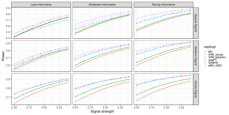
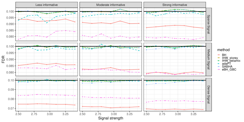
Figure C.1: Empirical FDR and power for $a_{f}=0.5$.

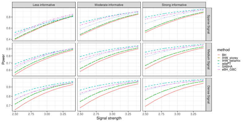
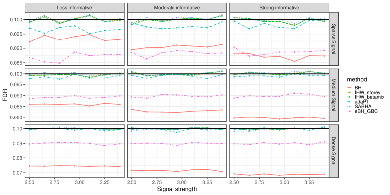
Figure C.2: Empirical FDR and power for $a_{f}=0$.

References

- Arias-Castro and Chen [2017] Ery Arias-Castro and Shiyun Chen. Distribution-free multiple testing. 2017.
- Barber and Candès [2015] Rina Foygel Barber and Emmanuel J Candès. Controlling the false discovery rate via knockoffs. The Annals of Statistics, 2015.
- Barber et al. [2020] Rina Foygel Barber, Emmanuel J Candès, and Richard J Samworth. Robust inference with knockoffs. 2020.
- Benjamini and Hochberg [1995] Yoav Benjamini and Yosef Hochberg. Controlling the false discovery rate: a practical and powerful approach to multiple testing. Journal of the Royal statistical society: series B (Methodological), 57(1):289–300, 1995.
- Boca and Leek [2018] Simina M Boca and Jeffrey T Leek. A direct approach to estimating false discovery rates conditional on covariates. PeerJ, 6:e6035, 2018.
- Bottomly et al. [2011] Daniel Bottomly, Nicole AR Walter, Jessica Ezzell Hunter, Priscila Darakjian, Sunita Kawane, Kari J Buck, Robert P Searles, Michael Mooney, Shannon K McWeeney, and Robert Hitzemann. Evaluating gene expression in c57bl/6j and dba/2j mouse striatum using rna-seq and microarrays. PloS one, 6(3):e17820, 2011.
- Cao et al. [2022] Hongyuan Cao, Jun Chen, and Xianyang Zhang. Optimal false discovery rate control for large scale multiple testing with auxiliary information. Annals of statistics, 50(2):807, 2022.
- Chouldechova [2017] Alexandra Chouldechova. Fair prediction with disparate impact: A study of bias in recidivism prediction instruments. Big data, 5(2):153–163, 2017.
- Dunn et al. [2023] Robin Dunn, Aaditya Ramdas, Sivaraman Balakrishnan, and Larry Wasserman. Gaussian universal likelihood ratio testing. Biometrika, 110(2):319–337, 2023.
- Efron [2005] Bradley Efron. Local false discovery rates, 2005.
- Ferreira and Zwinderman [2006] JA Ferreira and AH Zwinderman. On the benjamini–hochberg method. 2006.
- Genovese et al. [2006] Christopher R Genovese, Kathryn Roeder, and Larry Wasserman. False discovery control with p-value weighting. Biometrika, 93(3):509–524, 2006.
- Grünwald et al. [2020] Peter Grünwald, Rianne de Heide, and Wouter M Koolen. Safe testing. In 2020 Information Theory and Applications Workshop (ITA), pages 1–54. IEEE, 2020.
- Himes et al. [2014] Blanca E Himes, Xiaofeng Jiang, Peter Wagner, Ruoxi Hu, Qiyu Wang, Barbara Klanderman, Reid M Whitaker, Qingling Duan, Jessica Lasky-Su, Christina Nikolos, et al. Rna-seq transcriptome profiling identifies crispld2 as a glucocorticoid responsive gene that modulates cytokine function in airway smooth muscle cells. PloS one, 9(6):e99625, 2014.
- Hu et al. [2010] James X Hu, Hongyu Zhao, and Harrison H Zhou. False discovery rate control with groups. Journal of the American Statistical Association, 105(491):1215–1227, 2010.
- Ignatiadis and Huber [2021] Nikolaos Ignatiadis and Wolfgang Huber. Covariate powered cross-weighted multiple testing. Journal of the Royal Statistical Society Series B: Statistical Methodology, 83(4):720–751, 2021.
- Ignatiadis et al. [2016] Nikolaos Ignatiadis, Bernd Klaus, Judith B Zaugg, and Wolfgang Huber. Data-driven hypothesis weighting increases detection power in genome-scale multiple testing. Nature methods, 13(7):577–580, 2016.
- Ignatiadis et al. [2022] Nikolaos Ignatiadis, Ruodu Wang, and Aaditya Ramdas. E-values as unnormalized weights in multiple testing. arXiv preprint arXiv:2204.12447, 2022.
- Lei and Fithian [2018] Lihua Lei and William Fithian. Adapt: an interactive procedure for multiple testing with side information. Journal of the Royal Statistical Society Series B: Statistical Methodology, 80(4):649–679, 2018.
- Li and Barber [2019] Ang Li and Rina Foygel Barber. Multiple testing with the structure-adaptive benjamini–hochberg algorithm. Journal of the Royal Statistical Society Series B: Statistical Methodology, 81(1):45–74, 2019.
- McDonald et al. [2018] Daniel McDonald, Embriette Hyde, Justine W Debelius, James T Morton, Antonio Gonzalez, Gail Ackermann, Alexander A Aksenov, Bahar Behsaz, Caitriona Brennan, Yingfeng Chen, et al. American gut: an open platform for citizen science microbiome research. Msystems, 3(3):10–1128, 2018.
- Ren and Barber [2022] Zhimei Ren and Rina Foygel Barber. Derandomized knockoffs: leveraging e-values for false discovery rate control. arXiv preprint arXiv:2205.15461, 2022.
- Shafer [2021] Glenn Shafer. Testing by betting: A strategy for statistical and scientific communication. Journal of the Royal Statistical Society Series A: Statistics in Society, 184(2):407–431, 2021.
- Storey et al. [2004] John D Storey, Jonathan E Taylor, and David Siegmund. Strong control, conservative point estimation and simultaneous conservative consistency of false discovery rates: a unified approach. Journal of the Royal Statistical Society Series B: Statistical Methodology, 66(1):187–205, 2004.
- Sun and Cai [2007] Wenguang Sun and T Tony Cai. Oracle and adaptive compound decision rules for false discovery rate control. Journal of the American Statistical Association, 102(479):901–912, 2007.
- Sun et al. [2015] Wenguang Sun, Brian J Reich, T Tony Cai, Michele Guindani, and Armin Schwartzman. False discovery control in large-scale spatial multiple testing. Journal of the Royal Statistical Society Series B: Statistical Methodology, 77(1):59–83, 2015.
- Verma and Rubin [2018] Sahil Verma and Julia Rubin. Fairness definitions explained. In Proceedings of the international workshop on software fairness, pages 1–7, 2018.
- Vovk and Wang [2021] Vladimir Vovk and Ruodu Wang. E-values: Calibration, combination and applications. The Annals of Statistics, 49(3):1736–1754, 2021.
- Wang and Ramdas [2022] Ruodu Wang and Aaditya Ramdas. False discovery rate control with e-values. Journal of the Royal Statistical Society Series B: Statistical Methodology, 84(3):822–852, 2022.
- Xu and Ramdas [2023] Ziyu Xu and Aaditya Ramdas. More powerful multiple testing under dependence via randomization. arXiv preprint arXiv:2305.11126, 2023.
- Xu et al. [2021] Ziyu Xu, Ruodu Wang, and Aaditya Ramdas. A unified framework for bandit multiple testing. Advances in Neural Information Processing Systems, 34:16833–16845, 2021.
- Yun et al. [2022] Sooin Yun, Xianyang Zhang, and Bo Li. Detection of local differences in spatial characteristics between two spatiotemporal random fields. Journal of the American Statistical Association, 117(537):291–306, 2022.
- Zhang and Chen [2022] Xianyang Zhang and Jun Chen. Covariate adaptive false discovery rate control with applications to omics-wide multiple testing. Journal of the American Statistical Association, 117(537):411–427, 2022.
- Zhao and Zhou [2023] Haibing Zhao and Huijuan Zhou. -censored weighted benjamini-hochberg procedures under independence. Biometrika, page asad047, 2023.