Compensation of front-end and modulation delays in phase and ranging measurements for time-delay interferometry

Abstract

In the context of the Laser Interferometer Space Antenna (LISA), the laser subsystems exhibit frequency fluctuations that introduce significant levels of noise into the measurements, surpassing the gravitational wave signal by several orders of magnitude. Mitigation is achieved by means of time-shifting individual measurements in a data processing step known as time-delay interferometry (TDI). The suppression performance of TDI relies on accurate knowledge and consideration of the delays experienced by the interfering lasers. While considerable efforts have been dedicated to the accurate determination of inter-spacecraft ranging delays, the sources for delays onboard the spacecraft have been either neglected during TDI processing or assumed to be known. Contrary to these assumptions, analog delays of the phasemeter front end and the laser modulator are not only large but also prone to change with temperature and heterodyne frequency. This motivates our proposal for a novel method enabling a calibration of these delays on-ground and in-space, based on minimal functional additions to the receiver architecture. Specifically, we establish a set of calibration measurements and elucidate how these measurements are utilized in data processing, leading to the mitigation of the delays in the TDI Michelson variables. Following a performance analysis of the calibration measurements, the proposed calibration scheme is assessed through numerical simulations. We find that in the absence of the calibration scheme, the assumed drifts of the analog delays increase residual laser noise at high frequencies of the LISA measurement band. A single, on-ground calibration of the analog delays leads to an improvement by roughly one order of magnitude, while re-calibration in space may improve performance by yet another order of magnitude. Towards lower frequencies, ranging error is always found to be the limiting factor for which countermeasures are discussed.

I Introduction

During the past years several space missions aiming to detect gravitational waves have undergone intense study activities and are expected to soon enter the implementation phase. Among these missions are LISA Amaro-Seoane et al. (2017), a joint ESA-NASA mission, the Chinese TAIJI Luo et al. (2020) and TianQin Luo et al. (2016) missions, and the Japanese DECIGO mission Sato et al. (2017). The LISA constellation comprises three spacecraft (S/C) which form an approximately equilateral triangle of 2.5 million km arm-length and rotate around their common center in an Earth trailing orbit. Gravitational waves are detected through interferometric measurements of the relative distance changes between two freely floating test masses along each arm of the constellation, where each S/C transmits to and receives light from both its neighboring S/C Amaro-Seoane et al. (2017). The measurement for each arm is broken down into individual measurements of test-mass position relative to an optical bench (OB) and OB of one S/C relative to the OB of the opposite S/C, based on a concept referred to as “strap-down interferometry” Gath et al. (2009). Given that the strain sensitivity of the detector is proportional to the distance between S/C, attaining the targeted strain sensitivity of $10^{-21}$ within the 0.1 mHz to 1 Hz measurement frequency range requires the LISA constellation to extend across several million kilometers.
Owing to seasonally changing gravitational disturbances, the arm-lengths oscillate around their mean values with amplitudes of several thousand kilometers and relative velocities of around 15 m/s Otto (2015), leading to slowly varying Doppler shifts of the received laser frequency on the order of several megahertz. To ensure that the interferometric beat-note frequency (heterodyne frequency) remains within the detection bandwidth of the phasemeter, the lasers of all 6 optical links are frequency offset-locked relative to one another and require occasional changes of the frequency offset to account for the slow evolution of the heterodyne frequency over time, as defined in a “frequency offset plan” similar to the one defined for TAIJI Zhang et al. (2022). Despite using highly stable laser sources, the associated laser frequency noise transforms into large interferometric phase fluctuations across the arm-length which spoil the measurement performance. This physical show-stopper for long-distance heterodyne interferometry is overcome by a post-processing technique referred to as time-delay interferometry (TDI) Tinto and Dhurandhar (2021); de Vine et al. (2010). In TDI, laser noise is suppressed by time-shifting and linearly combining the interferometric measurements. The goal is to obtain synthetic measurement observables representing virtual equal arm-length interferometers. While there are many variants of TDI observables, each having their distinct advantages for gravitational wave analysis and instrument diagnostic, the $X,\leavevmode\nobreak\ Y,\leavevmode\nobreak\ Z$ observables, representing synthetic Michelson interferometers, are among the most frequently used ones in LISA science data processing research, and we will also adopt them in this paper. The Michelson variables allow completely suppressing laser frequency noise for unequal arm-lengths of a static constellation in TDI first generation (TDI 1.0) Tinto et al. (2002). However, accounting for changing arm-lengths and a rotating constellation required developing TDI second generation (TDI 2.0), where more complicated linear combinations of interferometric measurements are built to suppress laser noise to the required level. Both, TDI 1.0 and TDI 2.0 require the arm-lengths to be known so that the individual interferometric measurements can be shifted in time correctly. Consequently, any error in the arm-length estimate decreases the efficiency of the TDI suppression performance.

In order to supply TDI with the required inter S/C distance, referred to as “range”, auxiliary measurements are continuously performed for LISA Heinzel et al. (2011). These measurements rely on modulating the carrier phase of the transmitted laser beam with a pseudo-random noise (PRN) code sequence which is correlated with a local replica on the receiving S/C in order to determine the pseudo-range within the ambiguity range defined by the period of the PRN sequence in space ($\approx 300\,$km), which is a similar approach as the one used for GPS navigation systems in the radio-frequency regime. Regular coarse S/C position measurements from ground combined with orbit prediction of the S/C trajectories, allow for accurately resolving the ambiguity and determining the absolute ranges between S/C.

Note that for this scheme to work it is additionally required that the PRN code sequences modulated onto the transmitted beam on one S/C are synchronized to those of the local replica on the other S/C, which is the case if the clocks of all 3 S/C in the LISA constellation are synchronized to a common reference time. Ranging errors are closely related to clock synchronization errors, both leading to an offset in the alignment of individual measurements in the synthesis of TDI observables. Therefore, clock synchronization is generally required for synthesis of the virtual equal arm-length interferometers in TDI and performed as one of the post-processing steps in the LISA Initial Noise Reduction Pipeline (INReP) Otto (2015), although there has been a recent proposal for a TDI variant without the need for clock synchronization Hartwig et al. (2022).

Previous post-processing models have neglected or assumed perfect knowledge Reinhardt et al. (2024) of the delays in the phase measurement chain, including delays caused by the analog phasemeter front end and digital delays in the signal processing of the phasemeter back end, affecting not only the 6 long-arm interferometers measuring the inter-S/C distances but all 18 interferometers used in the LISA constellation. Additionally, the 6 auxiliary ranging measurements of the inter-S/C distance are affected by delays of the laser PRN modulation with respect to the S/C clock on the transmitter side as well as phasemeter front-end and back-end delays on the receiver side.

In this paper, we focus on these novel aspects and investigate how these delays can be accurately calibrated on ground and re-calibrated in space by only small functional additions to the current baseline of the receiver architecture. After identifying these delays in section II, we define a set of calibration measurements in section III. In section IV, we show how associated measurements are applied in a post-processing step and in TDI resulting in a compensation of these delays in the TDI Michelson variables. In section V, we assess the calibration and ranging performance due to sources of random noise, based on current baseline models of the LISA receiver architecture and physical signal parameters, and account for the errors in the simulations presented in section VI. Within these numerical simulations, the performance impact on TDI is assessed for 3 major cases: (1) the delays are not compensated, (2) the delays are only compensated based on calibration measurements performed on ground, and (3) the delays are compensated based on periodic calibration measurements performed in space. For case (2) the frequency noise suppression is increased by roughly one order of magnitude with respect to case (1) for higher measurement frequencies from 10 mHz to 1 Hz, while for case (3) the performance improves by roughly one order of magnitude with respect to case (2) for higher measurement frequencies from 100 mHz to 1 Hz. These findings clearly emphasize the importance of accurate delay calibration and adjustment of calibration parameters during the operational lifetime of LISA. At low frequencies of the LISA measurement band, performance is limited by the ranging error and possibilities are discussed to greatly improve the ranging performance by additional small modifications to the baseline of the receiver architecture.

II Measurement Principle and Delays

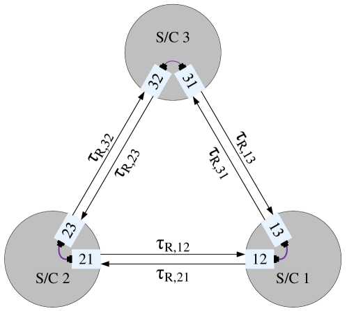
Figure 1: The LISA constellation consists of three S/Cs each hosting two OBs, highlighted in light blue. The light travel times among these OBs are indicated via the parameter $\tau_{\text{R}}$.

Figure 1 depicts a simplified schematic of the LISA constellation. Each S/C hosts two OBs and two associated free-falling test masses. The OBs will thereby be denoted as OB $ab$, where $a$ represents the S/C the OB is located and $b$ the S/C the laser of the OB is pointing to. In turn, each OB is equipped with three interferometers, cf. Fig. 2, leading to 18 interferometers for the full constellation. The long-arm interferometer (indicated via subscript L) measures relative distance fluctuations among the local OB and the OB of the remote S/C. The test-mass interferometer (indicated via subscript T) measures distance changes of the free-falling test mass of the local OB relative to the phase of the reference beam transmitted from the adjacent OB through a backlink fiber. Finally, the reference interferometer (indicated via subscript R) measures relative phase changes of the local reference beam against the reference beam of the adjacent OB without the test mass being part of the optical path.

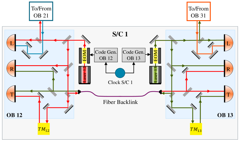
Figure 2: A simplified sketch indicating the interferometers present at S/C 1 is depicted. The S/C hosts two OBs. Each OB is equipped with three interferometers: the long-arm interferometer (L), the reference interferometer (R), and the test-mass interferometer (T). The photodiodes of these interferometers have been labeled with the respective letter. The OBs are connected via a fiber backlink highlighted in purple. For the sake of clarity, the beams of each laser have been distinctly color-coded. At the EOM lasers are modulated with a chip sequence supplied by the code generation unit, indicated via “Code Gen.”.

All of these 18 interferometers follow a common measurement principle, depicted in Fig. 3 Danzmann et al. (2011). Two laser beams with frequencies in the THz range ($\lambda=$ 1064 nm) are combined on an OB. The combined beams are processed by an analog front end. Interference of the beams at a QPD (quadrature photodiode) creates a beat note in the range of 6 to 24 MHz, depending on the relative S/C motion Barke et al. (2014). The resulting photocurrent serves as input to a transimpedance amplifier (TIA), which converts the photocurrent to a photovoltage. Thereby, the TIA is frequency selective, exhibiting a bandpass in the range of 5 to 25 MHz Fernández Barranco et al. (2018). Finally, an ADC (analog-to-digital converter) circuit transforms the signal to the digital domain, where the phase-readout is performed using an all-digital phase-locked loop (PLL) Shaddock et al. (2006); Barke et al. (2014).
These processing stages unavoidably introduce delays in the interferometric readouts, in addition to the delays arising from the individual routing of the interfering beams. In Fig. 3, phase delays of the long-arm interferometer, denoted with the symbol $\delta$, have been identified, similar to those described in Reinhardt et al. (2024). Each delay in Fig. 3 is demarcated by thick black lines, with corresponding labels provided at the end of each delay.

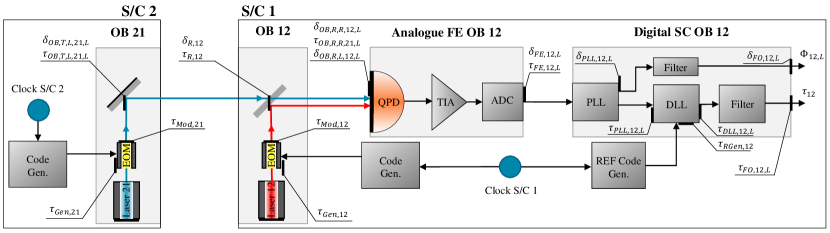
Figure 3: Schematic indicating the delays affecting the carrier phase and code read-out at the long-arm interferometer of OB 12. Individual phase and code delays are separated by thick black bars and labeled at the end of the individual delays with symbols $\delta$ and $\tau$, respectively.

Table 1: Phase delays $\delta$ encompassed by the laser beams for OB $ab$ and Interferometer $Z$ with $a,b\in\{1,2,3\}$, $a\neq b$ and $Z\in\{\text{L},\text{T},\text{R}\}$.

Interferometric phase delay	Symbol
OB delay at transmission (T) at local (L) S/C	$\delta_{\text{OB,T,L},ab,Z}$
OB delay at reception (R) at local (L) S/C	$\delta_{\text{OB,R,L},ab,Z}$
OB delay at reception (R) at remote (R) S/C	$\delta_{\text{OB,R,R},ab,Z}$
Phase delay of analog front end	$\delta_{\text{FE},ab,Z}$
PLL processing delay	$\delta_{\text{PLL},ab,Z}$
Output filtering delay	$\delta_{\text{FO},ab,Z}$
Ranging delay between S/C $b$ and S/C $a$	$\delta_{\text{R},ab}$
Phase delay due to test mass motion	$\delta_{\text{TM},ab}$
Fiber backlink among OB $ba$ and OB $ab$	$\delta_{\text{BL},ab}$

The interferometric read-outs of the test-mass and reference interferometer are delayed in a similar way except for the free space transmission of the remote laser. The individual delays of all interferometers are listed in Tab. 1. Equations 1 to 3 state the phase measurement $\Phi(t)$ on OB 12 for the three interferometers and detail how these delays affect the individual phase $\phi(t)$ of the interfering lasers.

$$\Phi_{12,L}(t +\delta_{\text{FE},12,\text{L}}+\delta_{\text{PLL},12,\text{L}}+\delta_{\text{FO},12,\text{L}})$$

$$=\phi_{21}(t-\delta_{\text{OB,T,L},21,\text{L}}-\delta_{\text{R},12}-\delta_{\text{OB,R,R},12,\text{L}})$$

$$-\phi_{12}(t-\delta_{\text{OB,R,L},12,\text{L}}),$$ (1)

$$\Phi_{12,T}(t +\delta_{\text{FE},12,\text{T}}+\delta_{\text{PLL},12,\text{T}}+\delta_{\text{FO},12,\text{T}})$$

$$=\phi_{13}(t-\delta_{\text{OB,T,L},13,\text{T}}-\delta_{\text{BL},12}-\delta_{\text{OB,R,R},12,\text{T}})$$

$$-\phi_{12}(t-\delta_{\text{OB,R,L},12,\text{T}}-\delta_{\text{TM},12}),$$ (2)

$$\Phi_{12,R}(t +\delta_{\text{FE},12,\text{R}}+\delta_{\text{PLL},12,\text{R}}+\delta_{\text{FO},12,\text{R}})$$

$$=\phi_{13}(t-\delta_{\text{OB,T,L},13,\text{R}}-\delta_{\text{BL},12}-\delta_{\text{OB,R,R},12,\text{R}})$$

$$-\phi_{12}(t-\delta_{\text{OB,R,L},12,\text{R}}).$$ (3)

The subscript of the phase measurement $\Phi(t)$ denotes the OB and the interferometer, separated by a comma. Similarly, the subscript of the laser phase $\phi$ denotes the OB the laser is associated with. Note that the time argument of the phase delays $\delta$ has been omitted in Eqs. 1 to 3 for readability. Moreover, phase delays appearing equally in both interfering lasers have been considered in the argument of the phase measurement $\Phi(t)$ . Interferometric readouts at the remaining OBs can be retrieved through a cyclic permutation of the numerical indices.

Besides the interferometric measurement, the long-arm interferometers allow for clock synchronization, absolute ranging, and data exchange among the S/Cs (summarized as auxiliary functions Heinzel et al. (2011)). These auxiliary functions are realized via low-depth phase modulations of the laser beam using an electro-optic modulator (EOM) Heinzel et al. (2011). Signals for clock synchronization are modulated as sidebands onto the main carrier. The frequency of the sidebands is chosen such that interference of the sidebands from the remote and local laser leads to a sideband/sideband beat note one megahertz away from the main beat note. This signal is processed separately but not further discussed here since it is not the focus of the ongoing discussion.
Absolute ranging and data transfer are employed using the principle of direct sequence spread spectrum (DSSS) Sutton et al. (2010); Esteban et al. (2011). PRN code sequences are modulated onto the carrier. In turn, data symbols are modulated onto these code sequences allowing for data transmission. Since most of the spectral energy of the code modulation lies outside the narrow bandwidth of the PLL, the chip sequences are not tracked by the PLL but appear as error in the signal. Consequently, the error channel (Q-channel) of the PLL is input to a delay-locked loop (DLL) Sutton et al. (2010); Esteban et al. (2011). The DLL correlates the incoming PRN code sequence with a local replica, which indicates the transmission time of the incoming chip sequence. Moreover, the sign of the correlation represents the data bit Esteban Delgado (2012).

Table 2: Code delays $\tau$ of the long-arm interferometer for OB $ab$ with $a,b\in\{1,2,3\}$ and $a\neq b$.

Code delay	Symbol
Code generation	$\tau_{\text{Gen},ab}$
Reference code generation	$\tau_{\text{RGen},ab}$
Code modulation	$\tau_{\text{Mod},ab}$
OB delay at transmission (T) at local (L) S/C	$\tau_{\text{OB,T,L},ab,Z}$
OB delay at reception (R) at remote (R) S/C	$\tau_{\text{OB,R,R},ab,Z}$
Ranging delay between S/C $b$ and S/C $a$	$\tau_{\text{R},ab}$
Code delay of analog front end	$\tau_{\text{FE},ab,\text{L}}$
PLL processing delay	$\tau_{\text{PLL},ab,\text{L}}$
DLL processing delay	$\tau_{\text{DLL},ab,\text{L}}$
Output filtering delay	$\tau_{\text{FO},ab,\text{L}}$

Similar to the interferometric phase measurements, the absolute ranging measurement is subjected to delays. The individual delays have been located in Fig. 3, denoted with symbol $\tau$, and identified in Tab. 2. As a result, the overall delay at the output filter of the DLL is given by

$$\tau_{12}(t +\tau_{\text{DLL},12,\text{L}}+\tau_{\text{FO},12,\text{L}})$$

$$=\tau_{\text{Gen},21}+\tau_{\text{Mod},21}+\tau_{\text{OB,T,L},21,\text{L}}+\tau_{\text{R},12}$$

$$+\tau_{\text{OB,R,R},12,\text{L}}+\tau_{\text{FE},12,\text{L}}+\tau_{\text{PLL},12,\text{L}}-\tau_{\text{RGen},12}.$$ (4)

Hereby, $\tau_{12}$ denotes the delay measured at the DLL based on the correlation of the incoming chip sequence with a local replica. Therefore, delays occurring after the measurement ($\tau_{\text{FO},12,\text{L}}$ and $\tau_{\text{DLL},12,\text{L}}$) appear as delays in the argument of $\tau_{12}$. The time argument of the code delays has been omitted in Eq. 4 for readability.
Since both, ranging and phase measurements, enter INReP, these delays must be precisely determined and adequately accounted for in the data processing of LISA.
Delays resulting from the OB ($\delta_{\text{OB}}$ and $\tau_{\text{OB}}$), are defined through the easily measurable geometric optical path-length differences (OPDs) on the OB. The latter is made from Zerodur and exhibits ultra-stable behavior so that any changes in these OPDs are completely negligible. Similarly, digital delays ($\delta_{\text{PLL},12,Z},\delta_{\text{FO},12,Z}$ with $Z\in\{\text{L},\text{T},\text{R}\}$ and $\tau_{\text{Gen},21},\tau_{\text{RGen},12},\tau_{\text{PLL},12,\text{L}},\tau_{\text{DLL},12,\text{L}},\tau_{\text{FO},12,\text{L}}$) can be calibrated via on-ground simulations. This is particularly important for the delay acting on the PRN sequences resulting from the sequential PLL-DLL architecture Euringer et al. (2023); Sutton et al. (2010). Finally, the deviation of the test mass from its nominal position is expected to be on the order of $\approx 10^{-4}$ m, resulting in a sub-picosecond delay. This delay, denoted as $\delta_{\text{TM},12}$ in Eq. 2, is significantly smaller in magnitude compared to the delays considered hereafter and omitted in the following.
At this point, we emphasize that clock differences among the S/C enter the phase measurement via the ADC conversion and the ranging measurement in the generation of the PRN code and the reference code. These differences are addressed separately, in particular via the clock jitter transfer based on sideband/sideband beat notes, and have been extensively studied in Reinhardt et al. (2024). Moreover, it has been shown that these delays can be addressed separately in a stand-alone post-processing step Hartwig et al. (2022). Consequently, these delays are assumed to be known and adequately suppressed.
In the following, we will comprise the aforementioned delays, namely delays from the OB, digital delays, and delays attributed to the clock differences, as “known delays” separating them from the front-end and modulation delays.
Despite the high stability of the phasemeter front end, small variations are expected to occur due to (1) the variation of the heterodyne frequency within the large receiver bandwidth (6 to 24 MHz) and due to (2) the seasonal changes in the environmental temperatures, as well as the expected ground-to-orbit (GTO) shift. As discussed above, the heterodyne frequency changes as a consequence of the slowly varying Doppler-shift and occasional reconfiguration of the offset-locking frequency and the temperature changes due to variation of the orbital parameters. Taking these effects into account and based on a simplified model of the stable front end shown in Fig. 3, we expect the mean front-end delays to be around 20 ns with a variation on the order of $\pm$5 ns over long timescales of several months. In addition, ranging measurements are affected by the modulation delay, which is exposed to similar drifts. On-ground calibration of these analog delays is complex and time-consuming. Furthermore, on-ground calibrations are prone to potential errors and likely to change due to GTO and temperature changes in orbit. Consequently, we seek a possibility to accurately calibrate and re-calibrate these delays.

III Calibration Measurement

In establishing a calibration scheme we first note that ranging measurements of the long-arm interferometer rely on the principle of PRN codes modulated onto the carrier with a small modulation depth Esteban Delgado (2012). As a result, the (main) power of the PRN codes is in close vicinity to the carrier power spectrum. In addition, carrier and code signal of the long-arm interferometer are processed by the identical analog front-end electronics until digitization. Assuming a sufficiently flat transfer function of the front-end electronic around the carrier Fernández Barranco et al. (2018), the front-end delay of the phase $\delta_{\text{FE},12,\text{L}}$ of the long-arm interferometer and the code $\tau_{\text{FE},12,\text{L}}$ are comparable, i.e. $\delta_{\text{FE},12,\text{L}}\approx\tau_{\text{FE},12,\text{L}}$. In fact, this relation holds exactly for phase components up to quadratic order around the carrier, since the code spectrum is symmetrically spread around the carrier. Based on the relation, additional ranging measurements can be introduced to determine the modulation delays and the front-end delays of all interferometers. These additional measurements require small modifications to the current baseline, which will be addressed in the subsequent section V.

As indicated in Fig. 2, the PRN modulation of each laser is performed before the laser output is split into one part used for local interferometry and another part that is transmitted to the remote S/C Barke et al. (2014). Hence, the beat notes of the interferometers are modulated by the PRN codes of both, the laser associated with the respective OB, which we refer to as “local laser”, as well as the PRN code from another OB, which we refer to as “remote laser”. The “remote laser” originates either from the adjacent OB of the same S/C for test-mass and reference interferometer, or from the OB of the remote S/C for the long-arm interferometer. Therefore, instead of correlating the incoming signal of the long-arm interferometer with the code of the distant S/C, a correlation with the local S/C can be performed. This measurement gives insight into the transmission path of the local PRN code Sutton et al. (2013). Neglecting the known delays including the digital delays and delays of the OB, which can simply be subtracted, the measurement reads

$$\text{CL}_{12,L}=\tau_{\text{FE},12,\text{L}}+\tau_{\text{Mod},12}.$$ (5)

Hereby, CL, short for “Calibration Local”, indicates a calibration (“C”) measurement, where the DLL correlates against the PRN code modulated onto the laser of the local (“L”) OB. In contrast, CR, short for “Calibration Remote”, indicates that the code modulated onto the laser of the remote (“R”) OB is considered. In other words, for performing the “CL” or “CR” measurement, the local or the remote code must be used by the reference code generator of the DLL, respectively. Finally, the subscript indicates the OB and the interferometer, separated by a comma.

In the same way, the incoming signal of the reference and test-mass interferometer features a PRN modulation and the error channel of the PLL reveals these chip sequences. Forwarding this signal to a DLL enables us to extend the application of ranging measurements to gain insight into the delays present in the read-out of the test-mass and reference interferometer. Following this approach, we introduce the additional calibration measurements

$$\text{CR}_{12,T} =\tau_{\text{BL},12}+\tau_{\text{FE},12,\text{T}}+\tau_{\text{Mod},13},$$ (6)

$$\text{CR}_{12,R} =\tau_{\text{BL},12}+\tau_{\text{FE},12,\text{R}}+\tau_{\text{Mod},13},$$ (7)

$$\text{CL}_{12,R} =\tau_{\text{FE},12,\text{R}}+\tau_{\text{Mod},12},$$ (8)

where similarly to Eq. 5, known delays have been omitted. The very same measurements can be performed on OB 13. Importantly, the fiber backlink connecting both OBs is bi-directional and requires reciprocal phase stability Fleddermann et al. (2018), which will be accounted for as $\tau_{\text{BL},12}=\tau_{\text{BL},13}$ in the following. As a result, the system of equations consists of 8 calibration measurement equations with 9 delays as variables. Although the system of equations is under-determined, it can be solved by expressing the delays in terms of one common delay. This delay can be arbitrarily chosen and shall be referred to as “reference delay” in the following. Exemplarily, Eq. 9 expresses the delays in terms of the front-end delay of the long-arm interferometer of OB 12, $\tau_{\text{FE},12,L}$, which serves as the “reference delay” of S/C 1.

$$\left(\begin{array}[]{c}\tau_{\text{FE},12,\text{T}}\\ \tau_{\text{FE},12,\text{R}}\\ \tau_{\text{FE},13,\text{L}}\\ \tau_{\text{FE},13,\text{T}}\\ \tau_{\text{FE},13,\text{R}}\\ \tau_{\text{Mod},12}\\ \tau_{\text{Mod},13}\\ \tau_{\text{BL},12}\end{array}\right)=\left(\begin{array}[]{c}-\text{CL}_{12,\text{L}}+\text{CL}_{12,\text{R}}-\text{CR}_{12,\text{R}}+\text{CR}_{12,\text{T}}+\tau_{\text{FE},12,\text{L}}\\ -\text{CL}_{12,\text{L}}+\text{CL}_{12,\text{R}}+\tau_{\text{FE},12,\text{L}}\\ \frac{1}{2}\left(-2\text{CL}_{12,\text{L}}+2\text{CL}_{13,\text{L}}+\text{CL}_{12,\text{R}}-\text{CL}_{13,\text{R}}-\text{CR}_{12,\text{R}}+\text{CR}_{13,\text{R}}\right)+\tau_{\text{FE},12,\text{L}}\\ \frac{1}{2}\left(-2\text{CL}_{12,\text{L}}+\text{CL}_{12,\text{R}}+\text{CL}_{13,\text{R}}-\text{CR}_{12,\text{R}}-\text{CR}_{13,\text{R}}+2\text{CR}_{13,\text{T}}\right)+\tau_{\text{FE},12,\text{L}}\\ \frac{1}{2}\left(-2\text{CL}_{12,\text{L}}+\text{CL}_{12,\text{R}}+\text{CL}_{13,\text{R}}-\text{CR}_{12,\text{R}}+\text{CR}_{13,\text{R}}\right)+\tau_{\text{FE},12,\text{L}}\\ \text{CL}_{12,\text{L}}-\tau_{\text{FE},12,\text{L}}\\ \frac{1}{2}\left(2\text{CL}_{12,\text{L}}-\text{CL}_{12,\text{R}}+\text{CL}_{13,\text{R}}+\text{CR}_{12,\text{R}}-\text{CR}_{13,\text{R}}\right)-\tau_{\text{FE},12,\text{L}}\\ \frac{1}{2}\left(-\text{CL}_{12,\text{R}}-\text{CL}_{13,\text{R}}+\text{CR}_{12,\text{R}}+\text{CR}_{13,\text{R}}\right)\end{array}\right)=\left(\begin{array}[]{c}m_{\text{FE},12,\text{T}}+\tau_{\text{FE},12,\text{L}}\\ m_{\text{FE},12,\text{R}}+\tau_{\text{FE},12,\text{L}}\\ m_{\text{FE},13,\text{L}}+\tau_{\text{FE},12,\text{L}}\\ m_{\text{FE},13,\text{T}}+\tau_{\text{FE},12,\text{L}}\\ m_{\text{FE},13,\text{R}}+\tau_{\text{FE},12,\text{L}}\\ m_{\text{Mod},12}-\tau_{\text{FE},12,\text{L}}\\ m_{\text{Mod},13}-\tau_{\text{FE},12,\text{L}}\\ m_{\text{BL},12}\end{array}\right)$$ (9)

In the expressions on the right surrounded by round brackets, measurement parameters $m$ with respective subscripts are introduced, which represent a combination of the individual calibration parameters. We note that all front-end delays follow the same scheme where the reference delay is added to all measurement parameters $m$. In contrast, the modulation delays consist of the difference between the measurement parameters $m$ and the reference delay. Finally, the fiber backlink delay is directly retrieved via the measurement parameter. Therefore, this delay is considered as “known” and omitted in the following discussion. Importantly, the calibration scheme allows expressing the modulation and front-end delays of all interferometers in terms of an individual measurement parameter $m$ and one common reference delay per S/C.

IV TDI Processing

TDI is a data post-processing technique designed to mitigate the impact of laser frequency noise by precisely time-shifting and linearly combining the interferometer measurements from multiple S/C. It is part of INReP, a crucial component within the LISA data analysis framework, responsible for the initial processing and filtering of the acquired data. INReP prepares the measurements for gravitational wave analysis. To assess the impact of the calibration scheme outlined in the preceding section on TDI, we provide a short summary of INReP and the TDI algorithm with reference to Otto (2015). For a more comprehensive understanding of INReP and the TDI algorithm, the reader is referred to Hartwig et al. (2022); Hartwig (2021); Houba et al. (2022a).
In section II, the delays present in the phase (Eqs. 1 to 3) and ranging (Eq. 4) measurements have been identified. In the following, we focus explicitly on the unknown analog delays, namely the front-end and the modulation delays, that have been addressed by the calibration scheme introduced in section III. The known delays in the ranging measurements can simply be subtracted from Eq. 4 and thus do not further affect the measurements. This is also the case for delays in the interferometric measurements (Eqs. 1 to 3), that appear equally in the beams of the interfering lasers. In fact, delays that occur exclusively in one laser must be examined separately. While this is the subject of ongoing investigations, it will not be further explored in the ongoing analysis.
Following this approach, Eqs. 10 to 12 illustrate the laser noise present in the measurements of the long-arm, test-mass, and reference interferometers introduced by Eqs. 1 to 3.

$$\Phi_{12,L}^{\text{p}}(t) =p_{21}(t-\tau_{\text{R},12}-\tau_{\text{FE},12,\text{L}})-p_{12}(t-\tau_{\text{FE},12,\text{L}}),$$ (10)

$$\Phi_{12,T}^{\text{p}}(t) =p_{13}(t-\tau_{\text{FE},12,\text{T}})-p_{12}(t-\tau_{\text{FE},12,\text{T}}),$$ (11)

$$\Phi_{12,R}^{\text{p}}(t) =p_{13}(t-\tau_{\text{FE},12,\text{R}})-p_{12}(t-\tau_{\text{FE},12,\text{R}}).$$ (12)

Hereby, the superscript p in the expressions $\Phi_{12,L}^{\text{p}}(t)$, $\Phi_{12,T}^{\text{p}}(t)$, and $\Phi_{12,R}^{\text{p}}(t)$, represents the impact of laser noise $p_{ab}(t)$ on the interferometric phase measurements. Moreover, phase delays have been expressed via the code delays, assuming a sufficiently flat transfer function in the vicinity of the carrier as explained in section III. The influence of laser noise on the remaining five OBs can be obtained from Eqs. 10 to 12 through a cyclic permutation of the indices.

In LISA, the set of interferometric measurements, along with the measured light travel times between the S/C are processed by INReP. Before the execution of TDI, additional algorithms are carried out to mitigate translational OB displacement noise, suppress clock noise, and reduce the number of laser noise sources from six to three. These algorithms are elaborated in Otto (2015). Importantly, all of the individual algorithms rely on linear combinations of the various phase measurements and shifting of these phase measurements in time. The shift in time is incorporated via a time-shift operator. In the following, we will provide an adapted definition of this time-shift operator, which allows for a compensation of front-end and modulation delays. Importantly, the compensation principle is demonstrated based on the time-shift operator itself, and since all of the individual algorithms incorporate this operator, compensation also applies to these algorithms.
In order to demonstrate the suppression of laser noise as given in Eqs. 10 to 12, it is sufficient to perform only the algorithm to reduce the number of laser noise sources from six to three before entering the TDI algorithm. However, the validity of the results persists when implementing the full INReP algorithm, as substantiated by arguments presented in the preceding paragraph. Equations 13 to 16 characterize the algorithm for the reduction of the number of laser noise sources from six to three required to obtain the TDI second-generation Michelson $X(t)$ channel.

$$\eta_{12}^{\text{p}}(t) =\Phi_{12,L}^{\text{p}}-D_{12}\left(\dfrac{\Phi_{23,R}^{\text{p}}-\Phi_{21,R}^{\text{p}}}{2}\right)$$ (13)

$$\eta_{13}^{\text{p}}(t) =\Phi_{13,L}^{\text{p}}-\dfrac{\Phi_{12,R}^{\text{p}}-\Phi_{13,R}^{\text{p}}}{2}$$ (14)

$$\eta_{21}^{\text{p}}(t) =\Phi_{21,L}^{\text{p}}-\dfrac{\Phi_{23,R}^{\text{p}}-\Phi_{21,R}^{\text{p}}}{2}$$ (15)

$$\eta_{31}^{\text{p}}(t) =\Phi_{31,L}^{\text{p}}-D_{31}\left(\dfrac{\Phi_{12,R}^{\text{p}}-\Phi_{13,R}^{\text{p}}}{2}\right)$$ (16)

Hereby, $D_{ba}$ represents the time shift operator that shifts a measurement performed on S/C $a$ by the time it takes for a signal to be received on S/C $b$.
TDI encompasses various combinations, such as Michelson, Sagnac, and further derivatives, offering distinct advantages in gravitational wave analysis Tinto et al. (2004). The TDI second-generation Michelson variable considered in this paper is a four-link combination requiring measurements from OB 12, OB 13, OB 21, and OB 31. The underlying algorithm is

$$X(t) =\eta_{13}^{\text{p}}-\eta_{12}^{\text{p}}+D_{A}\eta_{31}^{\text{p}}-D_{T}\eta_{21}^{\text{p}}$$

$$+D_{B}\eta_{12}^{\text{p}}-D_{U}\eta_{13}^{\text{p}}+D_{C}\eta_{21}^{\text{p}}-D_{V}\eta_{31}^{\text{p}}$$

$$+D_{D}\eta_{12}^{\text{p}}-D_{W}\eta_{13}^{\text{p}}+D_{E}\eta_{21}^{\text{p}}-D_{X}\eta_{31}^{\text{p}}$$

$$+D_{F}\eta_{13}^{\text{p}}-D_{Y}\eta_{12}^{\text{p}}+D_{G}\eta_{31}^{\text{p}}-D_{Z}\eta_{21}^{\text{p}}.$$ (17)

The time argument has been omitted above for readability. Note that multiple, nested delays are necessary to effectively cancel laser noise. Thereby, the nested delay operator is defined as $D_{ab,cb}f(t)=D_{cb}D_{ab}f(t)$ and similar for $n$-fold delay operations. The delay arrangements have been summarized as letters for clarity. The definitions of the subscript delay letters can be found in Table 3 Houba et al. (2022b).

Table 3: Translation Table for the Delay Index Notation.

Index	Delays	Index	Delays
$A$	13	$W$	31,13,21,12
$T$	12	$E$	12,21,12,31,13
$B$	31,13	$X$	13,31,13,21,12
$U$	21,12	$F$	21,12,21,12,31,13
$C$	12,31,13	$Y$	31,13,31,13,21,12
$V$	13,21,12	$G$	13,21,12,21,12,31,13
$D$	21,12,31,13	$Z$	12,31,13,31,13,21,12

The current TDI processing considers the S/C as a point mass, which implies that all interferometric measurements per S/C are performed at the same location. The time-shift operator is thereby defined according to Hartwig (2021)

$$D_{ba}^{\text{ideal}}f(t):=f\left(t-\tau_{\text{R},ba}\right),$$ (18)

to evaluate an arbitrary measurement $f(t)$ of S/C $a$ at the time of reception on S/C $b$ with $a,b\in\{1,2,3\}$ and $a\neq b$. We refer to these generic indices since INReP processing takes into account measurements from all 3 S/C. Indeed, definition 18 yields a static time-shift operator, as it excludes the consideration of the time dependence in the ranging delay $\tau_{\text{R},ba}$. Nevertheless, we will demonstrate that the outcomes remain valid even when accounting for time-dependent ranging delays.
Definition 18 faces two problems when taking into account the analog delays in the phase and ranging measurements:

(1) The interferometric measurements and thus the laser noise are delayed by individual front-end delays, cf. Eqs. 10 to 12, which makes the consideration of S/C as a point mass incorrect. This circumstance can be addressed by incorporating the calibration scheme of Eq. 9, enabling the expression of individual front-end delays through a reference delay and an individual measurement parameter $m$. In the following, we shift all phase measurements by this individual measurement delay. Exemplary, for the laser noise of the test-mass interferometer of OB 12, cf. Eq. 11, this results in

$$\Phi_{12,T}^{\text{p}} (t+m_{\text{FE},12,T})$$

$$=p_{13}(t-\tau_{\text{FE},12,\text{T}}+m_{\text{FE},12,T})$$

$$-p_{12}(t-\tau_{\text{FE},12,\text{T}}+m_{\text{FE},12,T})$$

$$=p_{13}(t-(m_{\text{FE},12,\text{T}}+\tau_{\text{FE},12,\text{L}})+m_{\text{FE},12,T})$$

$$-p_{12}(t-(m_{\text{FE},12,\text{T}}+\tau_{\text{FE},12,\text{L}})+m_{\text{FE},12,T})$$

$$=p_{13}(t-\tau_{\text{FE},12,\text{L}})-p_{12}(t-\tau_{\text{FE},12,\text{L}}),$$ (19)

where we used the result of Eq. 9, row 1. Consequently, the interferometric measurements per S/C are delayed by a single reference delay and definition 18 would still be accurate.

(2) Knowledge about the distance $\tau_{\text{R}}$ among the S/C is obtained via the absolute ranging measurement $\tau_{ba}$ of the DLL, cf. Eq. 4, which is affected by additional delays. Omitting the known delays, the ranging measurement is given by

$$\tau_{ba}=\tau_{\text{Mod},ab}+\tau_{\text{R},ba}+\tau_{\text{FE},ba,\text{L}}.$$ (20)

Similar to the phase measurement, we can express the additional delays, i.e. the modulation and front-end delay, via a reference delay taking into account row 6 and row 3 of Eq. 9, respectively. This results in

$$\tau_{\text{Mod},ab} =m_{\text{Mod},ab}-\tau_{\text{FE},ac,\text{L}},$$ (21)

$$\tau_{\text{FE},ba,\text{L}} =m_{\text{FE},ba,\text{L}}+\tau_{\text{FE,}bd,\text{L}},$$ (22)

with $a,b,c,d\in\{1,2,3\}$ and $b\neq a\neq c,b\neq d$. Without loss of generality, we considered the front-end delays $\tau_{\text{FE},ac,\text{L}}$ and $\tau_{\text{FE,}bd,\text{L}}$ of the long-arm interferometers as the reference delays of S/C $a$ and $b$, respectively. Following this procedure, the measurement of Eq. 20 is shifted by the measurement parameters $m_{\text{Mod},ab}$ and $m_{\text{FE},ba,\text{L}}$ of Eq. 21 and Eq. 22, respectively. Therefore, we account for these known measurement parameters by defining a biased time-shift operator as

$$D_{ba}^{\text{bias}}f(t):=f(t-\tau_{ba}+m_{\text{Mod},ab}+m_{\text{FE},ba,\text{L}}).$$ (23)

At this point, we note that the time-shift operator $D_{ba}$ is applied only to an interferometric measurement performed on S/C $a$ to evaluate it at the time of reception onboard S/C $b$. Based on the mitigation of problem (1), all phase measurements of S/C $a$ are expressed in terms of one reference delay and application of the the biased time-shift operator $D_{ba}^{\text{bias}}$ yields

$$D_{ba}^{\text{bias}}f(t -\tau_{\text{FE},ac,\text{L}})$$

$$=f(t -\tau_{\text{FE},ac,\text{L}}-\tau_{ba}+m_{\text{Mod,ab}}+m_{\text{FE},ba,\text{L}})$$

$$=f(t -\tau_{\text{FE},ac,\text{L}}-\tau_{\text{Mod},ab}-\tau_{\text{R},ba}$$

$$-\tau_{\text{FE},ba,\text{L}}+m_{\text{Mod},ab}+m_{\text{FE},ba,\text{L}})$$

$$=f(t -\tau_{\text{FE},ac,\text{L}}-m_{\text{Mod},ab}+\tau_{\text{FE},ac,\text{L}}-\tau_{\text{R},ba}$$

$$-m_{\text{FE},ba,\text{L}}-\tau_{\text{FE,}bd,\text{L}}+m_{\text{Mod},ab}+m_{\text{FE},ba,\text{L}})$$

$$=f(t -\tau_{\text{R},ba}-\tau_{\text{FE,}bd,\text{L}}).$$ (24)

We observe, the biased time-shift operator applies the correct ranging delay but also changes the front-end delay to the S/C, where the measurement shall be evaluated. In fact, we can express the biased time-shift operator in terms of the ideal time-shift operator by combining Eq. 18 and Eq. 24,

$$D_{ba}^{\text{bias}}f(t-\tau_{\text{FE},ac,\text{L}})=D_{ba}^{\text{ideal}}f(t-\tau_{\text{FE,}bd,\text{L}}).$$ (25)

Importantly, nesting the time-shift operator results in

$$D_{cb}^{\text{bias}}D_{ba}^{\text{bias}}f(t-\tau_{\text{FE},ac,\text{L}})=D_{cb}^{\text{ideal}}D_{ba}^{\text{ideal}}f(t-\tau_{\text{FE},ce,\text{L}}).$$ (26)

Again the reference delay of S/C $c$ is arbitrarily chosen to be $\tau_{\text{FE},ce,\text{L}}$. Finally, the indices in Eqs. 23 to 26 are defined by $a,b,c,d,e\in\{1,2,3\}$ and $a\neq b\neq c,a\neq c\neq e,b\neq d$. Following this observation, we can conclude that by nested application of the biased time-shift operator, only the front-end delay of the S/C, where the measurement shall be evaluated at last, remains. In the following, we will refer to this last reference delay as the leading reference delay.
So far, the time-shift operator has been applied in a static manner, meaning that the delays $\tau$ are time-invariant, an assumption applied in TDI 1.0. In contrast, the dynamic time shift operator used for TDI 2.0 assumes a time variation in the distances among the S/Cs. Nesting of the dynamic time-shift operator results in additional reference delays in the argument of the function $f(t)$. However, as shown in appendix A, these additional contributions are on the order of femtoseconds. Hence, Eq. 26 also holds in good approximation for the dynamic time shift operator.

Based on the behavior of nested biased time-shift operators as given in Eq. 26, analysis of the biased time-shift operator on INReP can be readily performed. Closely inspecting the terms that constitute the TDI $X$ variable in Eq. 17, reveals that the leading reference delay is identical for every term, namely $\tau_{\text{FE},12,\text{L}}$.

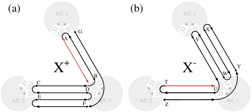
Figure 4: Schematic indicating the routing of the (nested) delay operators applied to the individual $\eta$-terms composing the TDI $X$ variable. The letters refer to the subscripts of the delay operators as given in Eq. 17 and indicate the start of the respective (nested) delay operator. The $\eta$-terms entering with a positive and negative sign have been separated in panels (a) and (b), respectively.

This observation can also be obtained graphically by illustrating the routing of the delay operators applied to the individual $\eta$-terms composing the TDI $X$ variable in Eq. 17. Hereby, terms entering with a positive and negative sign have been separated in Fig. 4(a) and (b), respectively. The subscript of the (nested) delay operators, as given in Tab. 3, indicates the start of the respective (nested) delay operator, while arrows represent the individual delay operators. Focusing on Fig. 4(a), we note that the paths created by the arrows are continuous and the (nested) delay operators share the same route. As a result, all (nested) delay operators end at the same S/C, namely at S/C 1. The same observation applies to Fig. 4(b). We can conclude that all terms entering the composition of the TDI $X$ variable are shifted by one common delay, the reference delay of S/C 1 $\tau_{\text{FE},12,\text{L}}$. Since, the remaining TDI Michelson variables $Y$ and $Z$ can be obtained from a cyclic permutation of measurement and delay indices one finds that these variables are delayed by the reference delay of S/C 2 and S/C 3, respectively. In this sense, the application of the calibration scheme translates the individual delays of the interferometers to a common delay per TDI Michelson variable and therefore – exact calibration provided – the individual delays do not affect the measurement performance.
Moreover, this principle also applies to higher-order Michelson variables, where the distinction from lower-order variables depends on the number of loops considered by the nested delay operators, while the leading reference delay remains unchanged Tinto and Dhurandhar (2023).

V Calibration performance

Utilizing the calibration method, the estimation of the delays relies on code measurements. The accuracy of these measurements depends on the code tracking configuration, in particular on the bandwidth and the discriminator of the DLL, and the signal-to-noise ratio.
The current baseline of LISA does not take into account calibration measurements.

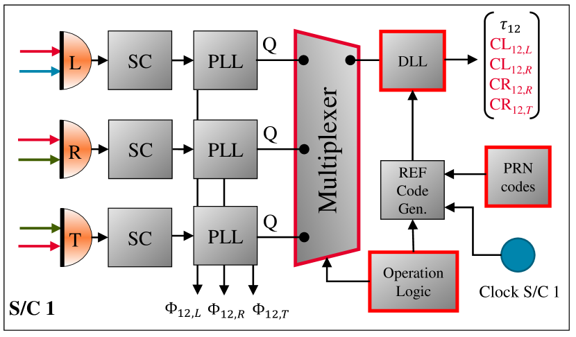
Figure 5: Schematic indicating via red frames the changes to the current baseline, necessary for the implementation of the proposed calibration scheme. The calibrations are controlled by an operation logic, which specifies the PRN code used in the reference code generator (“REF Code Gen.”) and the error channel (“Q”) that is routed to the DLL via a multiplexer. The processing electronic, TIA and ADC, is summarized as signal conditioning (“SC”).

Therefore, the least invasive method to perform these measurements is by means of time multiplexing, where all calibration measurements are performed using the DLL of the long-arm interferometer at fixed intervals. This avoids the need for additional DLLs but excludes the possibility of performing continuous calibrations. As outlined in section II, front-end delay variations are primarily attributed to temperature drifts, based on seasonal changes, and spectral drifts which are slowly varying on the timescale of weeks or months Barke et al. (2014). Consequently, intervals on the time scale of weeks seem to be sufficient. During the fixed calibration session the calibration of the long-arm, test-mass and reference interferometers of the S/C shall be performed sequentially. This process involves the transfer of the PLL error channel, denoted as “Q” in Fig. 5, from the interferometer used for calibration to the DLL situated at the phasemeter of the long-arm interferometer via a multiplexer.
In order to increase the calibration performance, only the laser whose transmission path is currently subject to calibration shall be code-modulated, i.e. the PRN code of the other interfering laser is constantly set to one. Moreover, the code used for the calibration shall be free of any data modulation, enabling a coherent early-late correlation in the DLL among the whole chip sequence. Finally, the calibration time per measurement is assumed to be 100 seconds.

Table 4: Baseline parameters

Parameter (Unit)	Symbol	Value
Modulation index (-)	$m_{\text{prn}}$	0.1
Chip period (ms)	$T_{c}$	0.001
Sampling rate (MHz)	$f_{s}$	80
Symbol period (ms)	$T_{s}$	1.024
Ranging bandwidth (Hz)	$B_{\text{DLL}}$	4
BOC(1,1) early-late spacing ($T_{c}$)	$\Delta_{\text{BOC}}$	0.2

It is worth noting that the absence of data modulation leads to the fact, that the sequential PLL-DLL architecture does not induce ranging variations. Instead, only a fixed ranging delay in the order of nanoseconds is present, which can be calibrated via simulations on ground and thus does not contribute to the calibration error Euringer et al. (2024). The performance of the calibration measurements is thus limited by two effects. (1) The incoming PRN sequences are contaminated with noise. The dominant noise source strongly depends on the interferometer. While the long-arm interferometer is limited by shot noise, this noise source plays a subordinate role in the test mass and reference interferometer, where stray light is one major noise source LISA Consortium (2021). The stray light contribution increases at low frequencies, however, this increase is counteracted by the high-pass behavior of the transfer function in the PLL error channel, which serves as input for the DLL Esteban Delgado (2012). Consequently, these noise contributions have been modeled as white noise. The error resulting from these contributions is denoted as $\sigma_{\text{n,c}}$ and can be estimated based on the analytical formulas of Betz Betz and Kolodziejski (2009a, b). Hereby, the subscript “c” denotes the coherent processing inside the DLL. (2) In addition, the DLL is working in the digital domain, causing performance degradation due to the granularity of the PRN code generator. This error is represented via $\sigma_{\text{o},\pm}$, where ($+$) denotes a maximum and ($-$) a minimum error and was derived in Euringer et al. (2023). Since both effects are uncorrelated the combined rms (root-mean-square) calibration error is given by

$$\sigma_{\text{c}} \approx\sqrt{\sigma_{\text{o},+}^{2}+\sigma_{\text{n,c}}^{2}},$$ (27)

where the application of $\sigma_{\text{o},+}$ leads to a conservative approach. Based on these assumptions and the parameters specified in Tab. 4, the calibration performance can be estimated. Thereby, LISA representative noise values from LISA Consortium (2021) have been taken into account for each interferometer. The resulting rms calibration errors are in the order of millimeters and dominated by the noise contributions $\sigma_{\text{n,c}}$ of the incoming signal. Individual calibration errors have been listed in Tab. 5.

Table 5: RMS errors

Measurement	RMS error
Calibration of long-arm interferometer	3.3 mm
Calibration of test-mass interferometer	1.3 mm
Calibration of reference interferometer	0.7 mm
Ranging	12 cm
Ranging when wiping local code	6.6 cm

In a similar manner, the ranging error of the long-arm interferometer can be estimated. However, two additional effects need to be considered. First of all, the interfering code of the local laser introduces an additional error $\sigma_{\text{i}}$, which has also been addressed by Betz Betz and Kolodziejski (2009a, b). Secondly, the sequential PLL-DLL processing in combination with data modulation of the chip sequences leads to ranging delay variations in the DLL Euringer et al. (2024). However, for the sampling period considered (80 MHz, cf. Tab. 4), these variations are much smaller than those arising from the granularity of the PRN code generator Euringer et al. (2023). Thus the ranging error is given by

$$\sigma_{\text{r}} \approx\sqrt{\sigma_{\text{o},+}^{2}+\sigma_{\text{n,n}}^{2}+\sigma_{\text{i,n}}^{2}}.$$ (28)

Thereby, the additional subscript “n” in $\sigma_{\text{n,n}}$ and $\sigma_{\text{i,n}}$ denotes the non-coherent processing of the DLL, which is necessary to remove the data modulation. Based on the parameters specified in Tab. 4, the rms ranging errors are in the order of several centimeters and listed in Tab. 5.

VI Simulation and Results

In order to assess the influence of the front-end and modulation delays and to verify the proposed calibration scheme, numerical simulations have been performed. The simulation comprises two stages: signal generation and signal processing. In the first stage, the interferometric measurements are generated according to Eqs. 10 to 12. Uncorrelated laser noise is considered for each OB as per the requirement. The light travel times are assumed to be time-varying, with relative S/C velocities of around 15 m/s Otto (2015). In the signal processing stage, all steps of INReP are executed, even though for the simulations in this paper, the noise sources to be suppressed by INReP, apart from laser noise, are set to zero. Front-end delays and modulation delays are taken into account in the generation of ranging measurements as well as interferometric signals. These delays are considered random but constant with respect to the simulation time, as described in section II. Therefore, the values of the individual front-end delays of the interferometers and the modulation delays have been drawn from a uniform distribution within an interval of 20$\pm$5 ns and 10$\pm$5 ns, respectively. Moreover, calibration errors $\sigma_{\text{c}}$ and ranging errors $\sigma_{\text{r}}$ are taken into account as specified in Tab. 5 unless otherwise noted. Signal processing is assessed for three primary scenarios regarding front-end and modulation delays: (1) uncompensated delays, (2) compensation of the mean delays, representing a single, ground-based calibration, and (3) compensation of the delays including variations, representing the execution of periodic calibration measurements performed in space. Depending on the simulation scenarios, the calibration scheme of section III is used by INReP to obtain the front-end and modulation delay estimates and mitigate their impact on residual laser noise in the TDI second-generation Michelson combination.

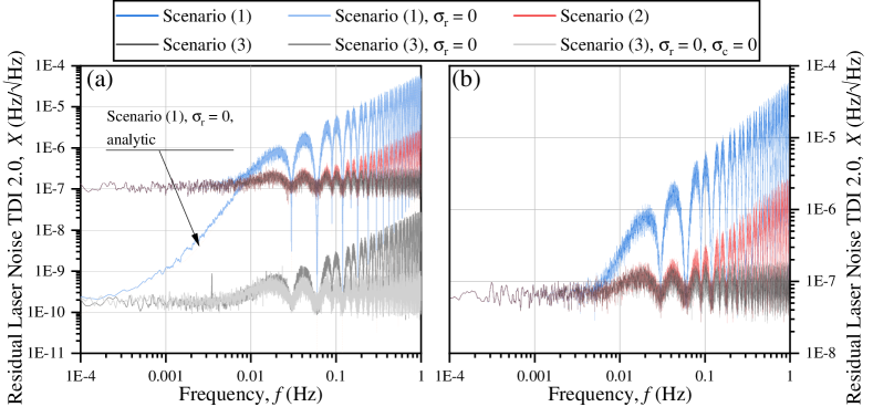
Figure 6: Residual laser noise in the TDI $X$ variable for 3 different scenarios. Panels (a) and (b) illustrate the results for the baseline ranging scheme and an improved ranging scheme, respectively.

The resulting residual laser noise for the TDI $X$ variable is depicted in Fig. 6(a). The gray curves consider a calibration of the front-end delays in space (scenario 3) as delineated in section III. Thereby, the light gray curve is free of any ranging or calibration errors, exhibiting a nearly flat noise spectrum of $\approx 2^{-10}\,\text{Hz}/\sqrt{\text{Hz}}$. The (mid) gray curve is affected by calibration errors leading to an increase in residual laser noise at frequencies $f>10$ mHz. The maximum increase of the laser noise is at the high frequencies of the measurement bandwidth by around one order of magnitude. Finally, the dark gray curve exhibits calibration and ranging errors. Here, the residual noise is increased by around three orders of magnitude over the whole measurement bandwidth, compared to the previous cases. Importantly, this exposes the ranging errors as the dominating noise source, if the calibration scheme is considered. In contrast, the red curve considers only a single, on-ground calibration of front-end and modulation delays, and inevitably neglects fluctuations in these delays (scenario 2). This leads to an increased laser noise resulting from the front-end and modulation delays manifesting as an increased residual noise at higher frequencies ($f>0.1$ Hz) by roughly one order of magnitude compared to scenario (3). Finally, the blue curves do not consider any mitigation of the front-end and modulation delays (scenario 1). Towards low frequencies, the dark blue curve approaches the noise level where a calibration is considered (overlapping with dark gray curve), but the noise level increases by two orders of magnitude towards higher frequencies compared to scenario (3). As a reference, the light-blue curve is free of any ranging error. The laser frequency noise is minimal at low frequencies, where front-end and modulation delays have little effect and the associated noise is negligible. At higher frequencies, the noise level strongly increases and exhibits a similar noise level as the dark blue curve, exposing modulation and front-end delays as dominant noise sources. This behavior is accurately described by the analytical solution represented by the orange dotted curve.

We note that the residual laser noise is dominated by the ranging errors when taking into account the proposed calibration scheme. Improvement of the ranging performance can be accomplished via different approaches:

(1) Time-delay interferometry ranging (TDIR) was initially introduced in Tinto et al. (2005) and aims at minimizing the rms power within specific TDI combinations to derive precise estimates of inter-S/C time delays. The estimates prove to be sufficiently accurate for effectively suppressing laser noise to a degree significantly lower than the secondary sources of noise. An alternative application of TDIR to estimate common-mode delays is given in Houba (2023). TDIR as a valuable crosscheck mechanism for evaluating residual PRN ranging offsets is described in Reinhardt et al. (2024).

(2) An optimization of the existing principle is obtained most easily by improving the carrier-to-noise ratio of the incoming signal of the DLL. The major noise contribution is the interfering code of the local laser Sutton et al. (2010). This noise source can be mitigated by wiping off the interfering code at the beginning of the DLL Sutton et al. (2013). This technique relies on two conditions. First of all, the delay of the local code is well-known based on the calibration measurement of the long-arm interferometer. Secondly, distortion of the chips due to the PLL processing can be incorporated via on-ground simulations Euringer et al. (2024); Sutton et al. (2010); Esteban Delgado (2012). We note that the presence of remote and local code does not change this processing as long as the PLL is working in the linear domain. Assuming perfect wiping of the local reference code, the ranging performance can be improved by around a factor of two, see last entry of Tab. 5. Interference code wiping has been experimentally demonstrated in Sutton et al. (2013), where suppression of the interfering chip sequence by a factor of $\approx$ 8 could be achieved, resulting in an rms ranging error of 0.06 m over a 0.5 Hz signal bandwidth.
For the improved ranging performance as stated in Tab. 5, the resulting residual laser noise of the TDI $X$ variable is depicted in Fig. 6(b). While the slope of the 3 scenarios remains identical to Fig. 6(a), the noise level is reduced by a factor of two at low frequencies. At higher frequencies, noise levels increase due to the uncompensated front-end and modulation delays for scenarios (1) and (2). This emphasizes the importance of re-calibration, as considered in scenario (3), which enables a reduction of the noise level at higher frequencies of the LISA measurement band. In fact, even much smaller ranging errors below 1 mm can be achieved by combining the ranging output with orbit prediction, for example using a Kalman filter as was used in Reinhardt et al. (2024). This further underscores the need for accurate calibration and compensation of front-end and modulation delays.

VII Conclusion

In this paper, we introduced a novel method for calibrating front-end and modulation delays in both, ground and space settings, allowing for the compensation of these delays in the TDI Michelson variables.
Based on a thorough identification of delays affecting ranging and phase measurements in all interferometers, delays were categorized into known and unknown delays, with known delays being easily determined through simulations or geometric path-length measurements. The unknown delays, specifically front-end and modulation delays, are difficult to mitigate because they require intricate calibrations and are expected to change in orbit.

To address this problem, a set of calibration measurements was proposed that relies on the fact that carrier phase and code chips are expected to experience very similar delays. These measurements, integrated with minimal functional additions to the receiver architecture, enable to express front-end and modulation delays in terms of one reference delay per S/C, resulting in three reference delays for the constellation. By incorporating this calibration set into the data processing pipeline, we demonstrated the separation of the three remaining reference delays in the three TDI Michelson variables. This led to the mitigation of front-end and modulation delays in the TDI Michelson variables.

Finally, the performance of the calibration measurements was determined based on the LISA receiver architecture and signal parameters. These results allowed a validation of the proposed calibration scheme using numerical simulations. Three scenarios were set up to evaluate the residual laser noise in the TDI variables for front-end and modulation delays being uncompensated, compensated via on-ground calibration, and compensated via additional re-calibration in space. In the absence of a calibration scheme, there is a significant increase in residual laser noise at frequencies above 10 mHz. On-ground calibration reduces the residual laser noise by one order of magnitude. Moreover, the increase in residual laser noise due to front-end and modulation delays shifts to frequencies above 100 mHz. Re-calibration in space eliminates any performance degradation caused by front-end and modulation delays. In this case, performance is limited by the ranging error, where improvement techniques have been delineated.

In conclusion, our findings underscore the critical importance of accurate delay calibration and the continuous adjustment of calibration parameters throughout the operational lifetime of LISA.

Appendix A Biased Dynamic Time-Shift Operator

In the following, we will derive an expression for the nested application of the dynamic time-shift operator considered in TDI 2.0 in the presence of front-end and modulation delays.

In TDI 1.0, the distances between S/C are presumed to remain constant over time. TDI 2.0 departs from this assumption by taking into account the temporal fluctuations in these distances. This is incorporated based on a dynamic time-shift operator $\mathcal{D}$ commonly defined as Otto (2015)

$$\mathcal{D}_{ba}^{\text{ideal}}f(t):=f\left(t-\tau_{\text{R},ba}(t)\right),$$ (29)

with $a,b\in\{1,2,3\}$ and $a\neq b$. Hereby, $\tau_{\text{R},ba}(t)$ denotes the time-dependent ranging delay among S/C $a$ and S/C $b$ at time $t$. The superscript “ideal” in the dynamic time-shift operator denotes that definition 29 considers the S/C as point masses. Nested application results in

$$\mathcal{D}_{cb}^{\text{ideal}}\mathcal{D}_{ba}^{\text{ideal}}f(t) =\mathcal{D}_{cb}^{\text{ideal}}f\left(t-\tau_{\text{R},ba}(t)\right),$$

$$=f\left(t-\tau_{\text{R},cb}(t)-\tau_{\text{R},ba}(t-\tau_{\text{R},cb}(t))\right),$$ (30)

and similar for $n$-fold delays. Indices in Eq. 30 are defined as $a,b,c\in\{1,2,3\}$ and $a\neq b\neq c$.

In analogous manner to the biased time-shift operator of Eq. 23, we define the biased dynamic time-shift operator as

$$\mathcal{D}_{ba}^{\text{bias}}f(t) :=f(t-\tau_{ba}(t)+m_{\text{Mod},ab}+m_{\text{FE},ba,\text{L}}).$$ (31)

Front-end and modulation delays and consequently the measurement parameters $m_{\text{Mod},ab}$ and $m_{\text{FE},ba,\text{L}}$ are assumed to be slowly varying on the timescale of weeks or months as described in section V. Moreover, the variation of these delays is expected to be on the order of $\pm$5 ns. The time-shifts induced by the ideal and the biased time-shift operator are on the order of tens of seconds Barke et al. (2014). On this time scale the variation of the parameter $m_{\text{Mod},ab}$ as well as $m_{\text{FE},ba,\text{L}}$ is on the order of $10^{-13}$ s, which is well below the stated calibration and ranging accuracy, cf. Table 5. Therefore, the time dependence is omitted for the measurement parameters $m_{\text{Mod},ab}$ and $m_{\text{FE},ba,\text{L}}$ in definition 31 and will be omitted for front-end and modulation delays in the ongoing discussion.
Nested application of the biased dynamic time-shift operator results in

$$\mathcal{D}_{cb}^{\text{bias}}\mathcal{D}_{ba}^{\text{bias}}f(t-\tau_{\text{FE},ac,\text{L}})$$

$$=\mathcal{D}_{cb}^{\text{bias}}f(t-\tau_{ba}(t)+m_{\text{Mod},ab}+m_{\text{FE},ba,\text{L}}-\tau_{\text{FE},ac,\text{L}})$$

$$=\mathcal{D}_{cb}^{\text{bias}}f\left(t-(\tau_{\text{Mod},ab}+\tau_{\text{R},ba}(t)+\tau_{\text{FE},ba,\text{L}})\right.$$

$$\left.+m_{\text{Mod},ab}+m_{\text{FE},ba,\text{L}}-\tau_{\text{FE},ac,\text{L}}\right)$$

$$=\mathcal{D}_{cb}^{\text{bias}}f\left(t-m_{\text{Mod},ab}+\tau_{\text{FE},ac,\text{L}}-\tau_{\text{R},ba}(t)\right.$$

$$\left.-m_{\text{FE},ba,\text{L}}-\tau_{\text{FE,}bd,\text{L}}+m_{\text{Mod},ab}+m_{\text{FE},ba,\text{L}}-\tau_{\text{FE},ac,\text{L}}\right)$$

$$=\mathcal{D}_{cb}^{\text{bias}}f(t-\tau_{\text{R},ba}(t)-\tau_{\text{FE,}bd,\text{L}})$$

$$=f\left(t-\tau_{cb}(t)\right.$$

$$-\tau_{\text{R},ba}(t-\tau_{cb}(t)+m_{\text{Mod},bc}+m_{\text{FE},cb,\text{L}})$$

$$\left.+m_{\text{Mod},bc}+m_{\text{FE},cb,\text{L}}-\tau_{\text{FE,}bd,\text{L}}\right)$$

$$=f\left(t-(\tau_{\text{Mod},bc}+\tau_{\text{R},cb}(t)+\tau_{\text{FE},cb,\text{L}})\right.$$

$$-\tau_{\text{R},ba}(t-(\tau_{\text{Mod},bc}+\tau_{\text{R},cb}(t)+\tau_{\text{FE},cb,\text{L}})$$

$$+m_{\text{Mod},bc}+m_{\text{FE},cb,\text{L}})$$

$$\left.+m_{\text{Mod},bc}+m_{\text{FE},cb,\text{L}}-\tau_{\text{FE,}bd,\text{L}}\right)$$

$$=f(t-\tau_{\text{R},ba}(t-\tau_{\text{R},cb}(t)-\tau_{\text{FE},ce,\text{L}})-\tau_{\text{R},cb}(t)-\tau_{\text{FE},ce,\text{L}}),$$ (32)

where we extensively employed the calibration scheme provided in Eq. 9 and indices are defined as $a,b,c,d,e\in\{1,2,3\}$ and $a\neq b\neq c,a\neq c\neq e,b\neq d$. To evaluate the additional shift by $\tau_{\text{FE},ce,\text{L}}$ in the argument of $\tau_{\text{R},ba}$ we perform a first-order Taylor expansion of $\tau_{\text{R},ba}$

$$\tau_{\text{R},ba}(t_{\text{ref}}-\tau_{\text{FE},ce,\text{L}}) \approx\tau_{\text{R},ba}(t_{\text{ref}})-\dot{\tau}_{\text{R},ba}(t_{\text{ref}})\tau_{\text{FE},ce,\text{L}}$$

$$\approx\tau_{\text{R},ba}(t_{\text{ref}})-\dfrac{\dot{L}_{\text{R},ba}(t_{\text{ref}})}{c}\tau_{\text{FE},ce,\text{L}}.$$ (33)

Hereby, $t_{\text{ref}}$ represents an arbitrary reference point in time and $c$ the speed of light. The parameter $\dot{L}_{\text{R},ba}(t_{\text{ref}})$ denotes the relative velocity along the line of sight among S/C $a$ and S/C $b$ which is around 15 m/s Otto (2015). As a result, $\tau_{\text{FE},ce,\text{L}}$ is weighted by the factor of $\dot{L}_{\text{R},ba}(t_{\text{ref}})/c\approx 10^{-8}$ in Eq. 33. Inserting Eq. 33 in Eq. 32 results in

$$\mathcal{D}_{cb}^{\text{bias}} \mathcal{D}_{ba}^{\text{bias}}f(t-\tau_{\text{FE},ac,\text{L}})$$

$$=f\left(t-\tau_{\text{R},ba}\left(t-\tau_{\text{R},cb}(t)\right)-\tau_{\text{R},cb}(t)\right.$$

$$\left.-\underbrace{\dfrac{\dot{L}_{\text{R},ba}\left(t-\tau_{\text{R},cb}(t)\right)}{c}\tau_{\text{FE},ce,\text{L}}}_{\approx 10^{-15}}-\tau_{\text{FE},ce,\text{L}}\right)$$

$$\approx f\left(t-\tau_{\text{R},ba}\left(t-\tau_{\text{R},cb}(t)\right)-\tau_{\text{R},cb}(t)-\tau_{\text{FE},ce,\text{L}}\right).$$ (34)

In the last line, we neglected the additional contribution of $\tau_{\text{FE},ce,\text{L}}$ which is on the order of femtoseconds and thus well below the stated calibration and ranging accuracy, cf. Table 5. Finally, combining Eq. 30 and Eq. 34, reveals the relation between nested application of the biased and the ideal dynamic time-shift operator

$$\mathcal{D}_{cb}^{\text{bias}}\mathcal{D}_{ba}^{\text{bias}}f(t-\tau_{\text{FE},ac,\text{L}}) \approx\mathcal{D}_{cb}^{\text{ideal}}\mathcal{D}_{ba}^{\text{ideal}}f(t-\tau_{\text{FE},ce,\text{L}}).$$ (35)

Comparison of Eq. 35 with Eq. 26 manifests that the relation between the nested application of the biased and the ideal time-shift operator is identical for the dynamic time-shift operator considered in TDI 2.0 and the static one considered in TDI 1.0.

References

- Amaro-Seoane et al. (2017) P. Amaro-Seoane, H. Audley, S. Babak, J. Baker, E. Barausse, P. Bender, E. Berti, P. Binetruy, M. Born, D. Bortoluzzi, et al., “Laser interferometer space antenna,” arXiv:1702.00786 (2017).
- Luo et al. (2020) Z. Luo, Y. Wang, Y. Wu, W. Hu, and G. Jin, “The Taiji program: A concise overview,” Prog. Theor. Exp. Phys. 2021 (2020), 10.1093/ptep/ptaa083, Art. no. 05A108.
- Luo et al. (2016) J. Luo, L.-S. Chen, H.-Z. Duan, Y.-G. Gong, S. Hu, J. Ji, Q. Liu, J. Mei, V. Milyukov, M. Sazhin, et al., “TianQin: a space-borne gravitational wave detector,” Class. Quantum Gravity 33, 035010 (2016).
- Sato et al. (2017) S. Sato, S. Kawamura, M. Ando, T. Nakamura, K. Tsubono, A. Araya, I. Funaki, K. Ioka, N. Kanda, S. Moriwaki, et al., “The status of DECIGO,” in J. Phys. Conf. Ser., Vol. 840 (IOP Publishing, 2017) p. 012010.
- Gath et al. (2009) P. F. Gath, D. Weise, H.-R. Schulte, and U. Johann, “Lisa mission and system architectures and performances,” J. Phys. Conf. Ser. 154, 012013 (2009).
- Otto (2015) M. Otto, “Time-delay interferometry simulations for the laser interferometer space antenna,” (2015).
- Zhang et al. (2022) J. Zhang, Z. Yang, X. Ma, X. Peng, H. Liu, W. Tang, M. Zhao, C. Gao, L.-E. Qiang, X. Han, and B. Liu, “Inter-spacecraft offset frequency setting strategy in the Taiji program,” Appl. Opt. 61, 837–843 (2022).
- Tinto and Dhurandhar (2021) M. Tinto and S. V. Dhurandhar, “Time-delay interferometry,” Living Rev. Relativ. 24, 1–73 (2021).
- de Vine et al. (2010) G. de Vine, B. Ware, K. McKenzie, R. E. Spero, W. M. Klipstein, and D. A. Shaddock, “Experimental demonstration of time-delay interferometry for the laser interferometer space antenna,” Phys. Rev. Lett. 104, 211103 (2010).
- Tinto et al. (2002) M. Tinto, F. B. Estabrook, and J. W. Armstrong, “Time-delay interferometry for LISA,” Phys. Rev. D 65, 082003 (2002).
- Heinzel et al. (2011) G. Heinzel, J. J. Esteban, S. Barke, M. Otto, Y. Wang, A. F. Garcia, and K. Danzmann, “Auxiliary functions of the LISA laser link: ranging, clock noise transfer and data communication,” Class. Quantum Gravity 28 (2011), Art. no. 094008.
- Hartwig et al. (2022) O. Hartwig, J.-B. Bayle, M. Staab, A. Hees, M. Lilley, and P. Wolf, “Time-delay interferometry without clock synchronization,” Phys. Rev. D 105, 122008 (2022).
- Reinhardt et al. (2024) J. N. Reinhardt, M. Staab, K. Yamamoto, J.-B. Bayle, A. Hees, O. Hartwig, K. Wiesner, S. Shah, and G. Heinzel, “Ranging sensor fusion in LISA data processing: Treatment of ambiguities, noise, and onboard delays in LISA ranging observables,” Phys. Rev. D 109, 022004 (2024).
- Danzmann et al. (2011) K. Danzmann, T. A. Prince, et al., LISA Assessment Study Report (Yellow Book), Tech. Rep. ESA/SRE(2011)3 (European Space Agency, 2011).
- Barke et al. (2014) S. Barke, N. Brause, I. Bykov, J. J. Esteban Delgado, A. Enggaard, O. Gerberding, et al., “LISA Metrology System - Final Report,” (2014).
- Fernández Barranco et al. (2018) G. Fernández Barranco, B. S. Sheard, C. Dahl, W. Mathis, and G. Heinzel, “A low-power, low-noise 37-mhz photoreceiver for intersatellite laser interferometers using discrete heterojunction bipolar transistors,” IEEE Sens. J. 18, 7414–7420 (2018).
- Shaddock et al. (2006) D. Shaddock, B. Ware, P. G. Halverson, R. E. Spero, and B. Klipstein, “Overview of the LISA Phasemeter,” AIP Conf. Proc. 873, 654–660 (2006).
- Sutton et al. (2010) A. Sutton, K. McKenzie, B. Ware, and D. A. Shaddock, “Laser ranging and communications for LISA,” Opt. Express 18, 20759–20773 (2010).
- Esteban et al. (2011) J. J. Esteban, A. F. García, S. Barke, A. M. Peinado, F. G. Cervantes, I. Bykov, G. Heinzel, and K. Danzmann, “Experimental demonstration of weak-light laser ranging and data communication for LISA,” Opt. Express 19, 15937–15946 (2011).
- Esteban Delgado (2012) J. J. Esteban Delgado, Laser Ranging and Data Communication for the Laser Interferometer Space Antenna, Ph.D. thesis, Universidad de Granada (2012).
- Euringer et al. (2023) P. Euringer, G. Hechenblaikner, F. Soualle, S. Delchambre, T. Ziegler, and W. Fichter, “Modeling of digital receiver-induced ranging bias variations in the context of high precision space-borne metrology systems,” in Proc. SPIE 12619, Modeling Aspects in Optical Metrology IX (2023) p. 126190A.
- Sutton et al. (2013) A. J. Sutton, K. McKenzie, B. Ware, G. de Vine, R. E. Spero, W. Klipstein, and D. A. Shaddock, “Improved optical ranging for space based gravitational wave detection,” Class. Quantum Gravity 30, 075008 (2013).
- Fleddermann et al. (2018) R. Fleddermann, C. Diekmann, F. Steier, M. Tröbs, G. Heinzel, and K. Danzmann, “Sub-pm non-reciprocal noise in the LISA backlink fiber,” Class. Quantum Gravity 35, 075007 (2018).
- Hartwig (2021) O. Hartwig, Instrumental modelling and noise reduction algorithms for the Laser Interferometer Space Antenna, Ph.D. thesis, Gottfried Wilhelm Leibniz Universität Hannover (2021).
- Houba et al. (2022a) N. Houba, S. Delchambre, T. Ziegler, and W. Fichter, “Optimal Estimation of Tilt-to-Length Noise for Spaceborne Gravitational-Wave Observatories,” J. Guid. Control Dyn. 45, 1–15 (2022a).
- Tinto et al. (2004) M. Tinto, F. B. Estabrook, and J. W. Armstrong, “Time delay interferometry with moving spacecraft arrays,” Phys. Rev. D 69 (2004).
- Houba et al. (2022b) N. Houba, S. Delchambre, T. Ziegler, G. Hechenblaikner, and W. Fichter, “LISA spacecraft maneuver design to estimate tilt-to-length noise during gravitational wave events,” Phys. Rev. D 106 (2022b), Art. no. 022004.
- Tinto and Dhurandhar (2023) M. Tinto and S. Dhurandhar, “Higher-order Time-Delay Interferometry,” (2023), arXiv:2307.07585 [gr-qc] .
- Euringer et al. (2024) P. Euringer, G. Hechenblaikner, F. Soualle, and W. Fichter, “Performance Analysis of Sequential Carrier- and Code-Tracking Receivers in the Context of High-Precision Spaceborne Metrology Systems,” IEEE Trans. Instrum. Meas. 73, 1–10 (2024).
- LISA Consortium (2021) LISA Consortium, “LISA Performance Model and Error Budget,” (2021), LISA-LCST-INST-TN-003. Technical Report 2.1, ESA.
- Betz and Kolodziejski (2009a) J. W. Betz and K. R. Kolodziejski, “Generalized Theory of Code Tracking with an Early-Late Discriminator Part I: Lower Bound and Coherent Processing,” IEEE Trans. Aerosp. Electron. Syst. 45, 1538–1556 (2009a).
- Betz and Kolodziejski (2009b) J. W. Betz and K. R. Kolodziejski, “Generalized Theory of Code Tracking with an Early-Late Discriminator Part II: Noncoherent Processing and Numerical Results,” IEEE Trans. Aerosp. Electron. Syst. 45, 1557–1564 (2009b).
- Tinto et al. (2005) M. Tinto, M. Vallisneri, and J. W. Armstrong, “Time-delay interferometric ranging for space-borne gravitational-wave detectors,” Phys. Rev. D 71, 041101 (2005).
- Houba (2023) N. Houba, Tilt-to-Length Noise Estimation and Reduction Algorithms for Spaceborne Gravitational-Wave Observatories, Fortschrittsberichte des Instituts für Flugmechanik und Flugregelung, Vol. 15 (Shaker Verlag, Düren, 2023) ISBN: 978-3-8440-9281-3.