Divergence-Free Flux Globalization Based Well-Balanced Path-Conservative Central-Upwind Schemes for Rotating Shallow Water Magnetohydrodynamics
Abstract
We develop a new second-order flux globalization based path-conservative central-upwind (PCCU) scheme for rotating shallow water magnetohydrodynamic equations. The new scheme is designed not only to maintain the divergence-free constraint of the magnetic field at the discrete level but also to satisfy the well-balanced (WB) property by exactly preserving some physically relevant steady states of the underlying system. The locally divergence-free constraint of the magnetic field is enforced by following the method recently introduced in [A. Chertock, A. Kurganov, M. Redle, and K. Wu, ArXiv preprint (2022), arXiv:2212.02682]: we consider a Godunov-Powell modified version of the studied system, introduce additional equations by spatially differentiating the magnetic field equations, and modify the reconstruction procedures for magnetic field variables. The WB property is ensured by implementing a flux globalization approach within the PCCU scheme, leading to a method capable of preserving both still- and moving-water equilibria exactly. In addition to provably achieving both the WB and divergence-free properties, the new method is implemented on an unstaggered grid and does not require any (approximate) Riemann problem solvers. The performance of the proposed method is demonstrated in several numerical experiments that confirm the lack of spurious oscillations, robustness, and high resolution of the obtained results.
Keywords: Rotating shallow water magnetohydrodynamics, divergence-free constraints, nonconservative hyperbolic systems of nonlinear PDEs, path-conservative central-upwind scheme, flux globalization based well-balanced scheme.
AMS subject classification: 65M08, 76W05, 76M12, 86-08, 35L65.
1 Introduction
Rotating shallow water magnetohydrodynamics (MHD) equations, also known as magnetic rotating shallow water (MRSW) equations, were introduced in the pioneering paper [33] as a model of the solar tachocline. Written in conservative form, the MRSW equations on the tangent plane to a rotating star/planet read as
| (1.1) | ||||
where and are the spatial variables in the plane, denotes time, represents the fluid thickness, is the horizontal velocity, denotes the horizontal magnetic field in units of velocity, denotes the tensor product, is the constant gravitational acceleration, is the time-independent bottom topography, denotes the vector obtained by rotating velocity by the angle , and is the Coriolis parameter. In what follows, the - and -components of vector fields will be often called zonal and meridional, respectively, according to the standard astro- and geophysical terminology. If the effects of the curvature are neglected, we get the simplest -plane approximation, where is constant. If the curvature is taken into account to the first order, we obtain the beta-plane approximation, with , . The model (1.1) represents the conservation of mass, momentum, and divergence-free magnetic flux in the presence of rotation and bottom topography, the latter two acting as specific sources. Topography was absent in the original formulation [33] but can be important, for instance, in geophysical applications. Note that in the absence of a magnetic field, the system becomes the standard rotating shallow water (RSW) model, abundantly studied in the physical and mathematical literature.
The MRSW model can be systematically derived from the full MHD equations for a magnetic rotating fluid in the Boussinesq and hydrostatic approximations, the latter being valid for large-scale motions, by vertical averaging [77]. A descendant MQG model for motions close to the magneto-geostrophic equilibrium, that is, an equilibrium between the pressure (magnetic plus hydrodynamic) and the Coriolis forces, follows from the MRSW equations by filtering the fast waves [77, 79]. At present, the MRSW and MQG models, as well as their variants, are used both in astrophysical (see, e.g., [60]) and geophysical (see, e.g., [65]) applications. The MRSW model allows us to describe the essential dynamical entities of the full MHD, such as (magnetized) vortices, (magneto-)inertia-gravity, Alfvén waves, and their interactions, and also turbulent regimes [60, 68]. It is well known (see, e.g., [51]) that the MHD equations admit shocks of various geometries and contact discontinuities, and this property is inherited by the MRSW model. Besides that, the MRSW equations admit Rossby waves, which arise in the configurations close to magneto-geostrophic equilibria in the presence of differential rotation and are of particular interest for applications; see, e.g., the review papers [29, 76]. In addition, exact steady-moving balanced vortex dipole solutions of the MQG equations, with a magnetic anomaly, either trapped inside or expelled from their cores, were recently found [50], and a question of their counterparts in the full MHD equations arise.
The present paper aims to develop a numerical scheme for (1.1), which would provide a reliable tool for investigating various aforementioned nonlinear dynamical processes and beyond. However, the construction of such a scheme has to rise to two main challenges. The first challenge is to ensure a well-balanced (WB) property, that is, to develop a scheme capable of exactly preserving (several) physically relevant steady states that correspond to an exact balance of flux-divergence and source terms in (1.1). Formulating a method that ensures the WB property is, however, nontrivial. For example, a straightforward, shock-capturing discretization can often result in spurious oscillations or spurious numerical waves that could be orders of magnitude larger than the small perturbation (of the steady state) to be captured. While using a very fine mesh may be able to fix these issues, such an approach would drastically increase computational time and may thus be impractical. For the standard RSW system, that is, (1.1) without magnetic field, several WB schemes were developed; see, e.g., [2, 5, 10, 14, 17, 23, 26, 55] and references therein.
In this paper, we develop a new WB scheme for the MRSW system (1.1) using a flux globalization approach introduced in [18, 12, 25, 32, 57] and recently successfully applied to a variety of systems of balance laws; see, e.g., [10, 11, 16, 17, 43, 44]. In this approach, both the source and nonconservative product terms are incorporated into the flux leading to an equivalent quasi-conservative system with a global flux. The resulting system is then integrated using a Riemann-problem-solver-free central-upwind (CU) scheme. The CU schemes were introduced in [42, 45, 46, 47, 48] as a robust “black-box” solver for general multidimensional systems of conservation laws and then were almost directly applied to the quasi-conservative systems with global fluxes in [10, 11, 16, 17, 18, 43, 44]. The CU schemes were extended to nonconservative hyperbolic systems in [15], where path-conservative CU (PCCU) schemes were introduced. The path-conservative technique has been recently incorporated into the flux globalization framework, and WB flux globalization based PCCU schemes have been introduced in [10, 11, 43]. These WB schemes are capable of exactly preserving a wide variety of steady states, including some discontinuous ones.
The second main challenge is the maintenance of the zero-divergence constraint for the magnetic flux, , at the discrete level. It is well-known that the enforcement of this constraint helps to prevent the appearance of nonphysical structures or spurious oscillations in the solutions; see, e.g., [3, 8, 52, 69]. A large variety of methods that preserve the divergence-free constraint in the context of the full MHD equations has been proposed; we refer the reader to, for instance, [19, 28, 30, 36, 54, 58, 75] and references therein. For the shallow water MHD, early efforts in discrete divergence preservation were introduced through constrained transport methods in [66, 21]. The main idea of constrained transport methods was to stagger the magnetic field in such a way that exactly preserves the divergence-free constraint. The constrained transport methods have since been further developed to be robust on unstaggered grids (see, e.g., [70]). Still, they are typically based on exact or approximate Riemann problem solvers. Another commonly used approach, known as the divergence cleaning [8], uses a Hodge decomposition to project the magnetic field into a divergence-free subspace and then to advect the divergence errors with the flow in such a way that does not cause accumulation. The divergence cleaning methods formulated for the shallow water MHD include, among others, Roe-type methods [38], conservation element/solution element (CE/SE) methods [1, 64], and a kinetic flux-vector splitting method [63]. These divergence cleaning methods, however, do not ensure an identically zero divergence, even though the divergence errors are controlled. A divergence-free finite volume evolution Galerkin method was introduced in [41], and divergence-free entropy stable methods were proposed in [27, 72]. In the latter works, the divergence constraint is enforced by including and discretizing an additional source term, known as a Janhunen source.
Several numerical methods, which are both WB and divergence-free, are available in the literature. In [7], a WB divergence-free method for one-dimensional (1-D) shallow-water MHD equations was constructed. In [81], a WB method was proposed, which employs a divergence cleaning approach to reduce but not completely diminish the discrete divergence. In addition, a high-order entropy stable finite-difference divergence-free method proposed in [27] is WB in the sense that it is capable of exactly preserving “lake-at-rest” steady states in both one and two dimensions.
In this paper, we construct a divergence-free flux globalization based WB PCCU scheme for MRSW system (1.1). Thanks to a flux globalization technique from [43], which we modify to treat the MRSW equations, our scheme preserves not only simple “lake-at-rest” steady states, but also some of the moving-water equilibria. The divergence-free constraint is enforced using the technique we have recently introduced in [19]. Namely, we use (i) a Godunov-Powell modified version of the MRSW system (1.1); (ii) additional equations obtained by spatially differentiating the magnetic field equations in (1.1); and (iii) reconstruction adjustments for magnetic field variables. The resulting method is successfully tested on a number of both 1-D and two-dimensional (2-D) numerical examples and produces accurate and non-oscillatory results.
The paper is organized as follows. In §2, we present the WB PCCU divergence-free method for the 1-D MRSW system: we first discuss the MRSW model modifications (§2.1) and then introduce a new 1-D numerical method (§2.2). We organize §3 the same as §2: we first present the 2-D MRSW model modifications (§3.1) and then introduce a new 2-D numerical method (§3.2). In §4.1 and §4.2, we show the 1-D and 2-D numerical experiments, respectively. We make our concluding remarks in §5.
2 1-D Well-Balanced PCCU Scheme for MRSW Equations
2.1 Governing Equations
In the 1-D case, the MRSW system (1.1) reduces to
| (2.1) | ||||
Note that this system is sometimes referred to as the 1.5-D MRSW system; see, for example, [79]; as translational symmetry is imposed on the 2-D model in the -direction. In other words, the -dependence is discarded, but we keep the -components of the vector fields and to have a model that includes rotational effects. In this paper, we will refer to the system (2.1) as the 1-D MRSW model. In addition, notice that (2.1) satisfies the divergence-free constraint , which in the 1-D case simplifies to
| (2.2) |
as long as this condition is satisfied initially.
Before discretization, we make several adjustments to the system (2.1) that will make it easier to devise a scheme that exactly preserves both the divergence-free constraint (2.2) and can exactly preserve some of the steady states of (2.1). We start modifications by adjusting the system (2.1) to include the additional Godunov-Powell source terms (see, e.g., [20, 22, 39, 41, 72]):
| (2.3) | ||||
which can be written in the following vector form:
| (2.4) |
where and
| (2.5) |
Note that the additional terms are theoretically zero due to (2.2). However, including them helps to enforce the divergence-free condition (2.2) at the discrete level.
There are several ways to discretize the Godunov-Powell modified MRSW system (2.3) in a divergence-free way (see, e.g., [31, 37, 71] and related works for ideal MHD [61, 62, 73, 74]). In this paper, we follow [19] and achieve this goal by first introducing the new variable that satisfies the additional evolution equation
| (2.6) |
which is obtained by taking the -derivative of the induction equation in (2.3), and then numerically solving the augmented system (2.4)–(2.6). While this system is set in a way that makes it relatively easy to design a scheme that preserves the divergence-free constraint (2.2), its direct discretization does not necessarily lead to a WB scheme.
One can show that the system (2.4)–(2.6) possesses steady-state solutions that satisfy
| (2.7) |
with being an arbitrary number and
| (2.8) |
Furthermore, since both and are constants at equilibrium, (2.8) is, in fact, a linear system for and , which can be easily solved to obtain
| (2.9) |
Since , one can integrate (2.9) to obtain
| (2.10) |
where and are constants of integration.
In order to derive a WB scheme capable of exactly preserving steady states satisfying (2.7), (2.9), we use the flux globalization approach. To do so, we rewrite the augmented system (2.4)–(2.6) in the following quasi-conservative form:
| (2.11) |
with the global variables :
| (2.12) |
whose nonzero components are
| (2.13) | ||||
Note that the derivative of the global flux, , can be rewritten in the following matrix-vector form:
where , is the vector of equilibrium variables with defined in (2.7), and
| (2.14) |
At the steady states, or, equivalently, , where denotes the equilibrium variables, which are used in WB finite-volume methods to perform piecewise polynomial interpolations/reconstructions. The obtained piecewise polynomial approximant will be exact when the discrete data are at a steady state. Typically, equilibrium variables are constant at steady states, but unlike similar situations in [10, 11, 43], where relations similar to (2.9) were established, only three of the components of (, , and ) are constant at the steady states. At the same time, and are either linear (if the Coriolis parameter ) or quadratic (if ) functions of ; see (2.10). Such functions can, however, be exactly recovered using piecewise polynomial interpolations/reconstructions, and therefore, the WB scheme that will be developed in §2.2 will rely on the reconstruction of instead of .
2.2 Numerical Method
This section describes the 1-D semi-discrete divergence-free flux globalization based WB PCCU scheme for (2.11)–(2.13). We start by introducing a 1-D uniform Cartesian grid with finite-volume cells of size , . Throughout §2.2, we will use the lower boundary of integration to evaluate all of the global quantities.
We assume that a numerical solution realized in terms of its cell averages,
is available at a certain time . Note that, for the sake of brevity, we omit the time dependence of and other indexed quantities here and throughout the paper. Within a semi-discrete framework, the solution is evolved in time by solving the following system of ODEs:
where
| (2.15) |
are the WB PCCU numerical fluxes from [43], is given in (2.11)–(2.13), and and are two slightly different approximations of the one-sided point values of at ; see §2.2.1 for details. In addition, in (2.15) denote the one-sided local speeds of propagation, which can be estimated using the largest and smallest eigenvalues of the matrix as follows:
where the point values , , and will be specified in the next section.
2.2.1 Well-Balanced Reconstruction
The development of the proposed WB scheme hinges on reconstructing the equilibrium variables instead of the conservative variables . We therefore first need to compute the discrete values out of the available cell averages :
| (2.16) |
where and the values are computed using the trapezoidal rule within the following recursive formula:
| (2.17) |
where , , and is determined by the boundary conditions.
Now equipped with the values , , and , we compute the point values , , and at the cell interfaces . For the fields , , , and we perform a generalized minmod reconstruction described in Appendix A, while for we replace the slope in (A.1) with . The latter is motivated by [19] and is needed to ensure that the discrete divergence-free condition (2.2) is locally satisfied as long as this condition is held at .
Recall that while three of the equilibrium variables, , , and , are constant at the steady states, the remaining two equilibrium variables, and , are either linear (if ) or quadratic (if ) functions. In the former case, we use the piecewise linear generalized minmod reconstruction, while in the latter case, we utilize the fifth-order WENO-Z interpolation briefly described in Appendix B. In both cases, the implemented reconstructions recover the exact point values and at the steady states satisfying (2.10).
Now that the point values of the equilibrium variables are available, we compute the corresponding values as follows. We first compute the water surface values , perform the piecewise linear reconstruction described in Appendix A to obtain the point values , which, in turn, are used to set or . We then exactly solve (following [16, 40]) the cubic equations
| (2.18) |
which arise from the definition of in (2.7) and the global terms are evaluated using the midpoint rule within the following recursive formula:
| (2.19) |
If the equation for in (2.18)–(2.19) has no positive solutions, we set , while if it has more than one positive root, we single out a root corresponding to the physically relevant solution by selecting the root closest to . A similar algorithm is implemented to obtain in (2.18)–(2.19). Once are obtained, we compute
Next, we explain how to obtain the point values that appear in the numerical diffusion terms on the right-hand side (RHS) of (2.15). These modified point values are needed to ensure that at steady states, and hence the numerical diffusion terms in (2.15) vanish. This, in turn, guarantees the WB property of the designed scheme as proven in §2.2.3.
We follow [43] and first set , , and as , , and are constant at steady states. The values are obtained by solving the following modified versions of the nonlinear cubic equations in (2.18):
| (2.20) |
where there only change made is the replacement of with .
Equations (2.20) are solved exactly the same way equations (2.18) have been solved, and it is easy to see that whenever the data is locally at steady state, that is, if , , and , then .
Finally, we compute , .
2.2.2 Well-Balanced Evaluation of the Global Fluxes
In order to compute the numerical fluxes (2.15), we first use the cell interface point values computed in §2.2.1 to evaluate the discrete values of the global fluxes appearing in (2.11)–(2.13):
| (2.21) |
where denote the numerical approximation of the integrals appearing in (2.13). In order to ensure the resulting method is WB and since the integrals contain the nonconservative products, we follow [10, 11, 43] and use the path-conservative technique to evaluate using the following recursive formulae:
| (2.22) |
where and are found using appropriate quadratures for
Here, is a certain path connecting the states and at the cell interface . In order to ensure the WB property, we use a line segment connecting the left and right cell interface values of the equilibrium variables:
which corresponds to a particular path , whose detailed structure is only given implicitly; see [43] for details. We then use the technique introduced in [43] to compute
and
| (2.23) |
2.2.3 Well-Balanced Property
Theorem 2.2.
Proof.
Assume that at a certain time level, the computed solution is at the steady state satisfying (2.7) and (2.10) at the discrete level, namely:
| (2.24) |
where , , and are constants, and
| (2.25) |
In order to show that the steady states are preserved exactly, we must show that
| (2.26) |
We begin with the first equality in (2.26), which is, according to (2.21), equivalent to
which then can be rewritten using the definition of in (2.22), (2.23) as
We then proceed with proving that , which, similarly to the first equality in (2.26), can be equivalently rewritten as
| (2.27) |
The assumptions in (2.24) immediately imply that the equalities in (2.27) are valid for the first, third, and fifth components. However, proving the second and fourth components in (2.27) is less straightforward since the profiles of and are (generally) nonconstant when at steady states.
The second and fourth components of (2.27) read as
Using (2.24), the above can be simplified to obtain that (2.27) is equivalent to
| (2.28) | ||||
Finally, we recall that our piecewise linear (in the case when ) or piecewise quadratic (in the case when ) reconstruction of and is exact when the computed solution is at the discrete steady state. Therefore, in this case, we use (2.10) to obtain
which we substitute into (2.28) to verify that the equalities there are true. This completes the proof of the theorem. ∎
3 2-D Well-Balanced PCCU Scheme for MRSW Equations
3.1 Governing Equations
In this section, we extend our studies to the 2-D MRSW system. As in the 1-D case, we modify the 2-D MRSW system by including the Godunov-Powell source terms to help enforce the divergence-free constraint at the discrete level. The adjusted 2-D system then reads as
| (3.1) | ||||
It is easy to show that a solution of (3.1) satisfies the 2-D divergence-free constraint
| (3.2) |
as long as it is met initially. The system (3.1) can be rewritten in the following vector form:
| (3.3) |
where and
| (3.4) | ||||
Notice that the additional terms are theoretically zero due to (3.2), but their inclusion help to enforce the divergence-free condition in (3.2) at the discrete level.
As in the 1-D case, we use the idea introduced in [19] to locally preserve the discrete divergence-free constraint: We introduce the new variables and that satisfy the additional evolution equations for the magnetic field derivatives
| (3.5) | ||||
which are obtained by differentiating the - and -equation in (3.1) with respect to and , respectively. As shown in [19], it is relatively easy to discretize the augmented system (3.3)–(3.5) and design a numerical scheme that preserves the divergence-free constraint (3.2). However, the resulting scheme will not necessarily be WB.
In order to derive a WB scheme for the augmented system (3.3)–(3.5), we follow the 2-D flux globalization approach recently introduced in [9] and rewrite the studied system in the following quasi-conservative form:
| (3.6) | ||||
with the global variables and :
| (3.7) | ||||
whose nonzero components are
| (3.8) | ||||
and and are arbitrary numbers.
Note that as in the 1-D case, the corresponding derivatives of the global fluxes, and , can be rewritten in the following matrix-vector forms:
| (3.9) | ||||
where
| (3.10) |
and and with
| (3.11) | ||||||
Note that general steady states of the 2-D MRSW system satisfy or, equivalently, . It is, however, very hard to design a WB numerical method capable of preserving general (genuinely 2-D) equilibria. The WB numerical method, which we present in the next section, is constructed to preserve the following families of quasi 1-D steady states exactly:
| (3.12) |
and
| (3.13) |
for each of which both and .
3.2 Numerical Method
In this section, we extend the proposed 1-D divergence-free flux globalization based WB PCCU scheme to the 2-D MRSW system (3.6)–(3.8).
We assume that at a certain time , the numerical solution realized in terms of its cell averages
is available. Here, are the 2-D finite volume cells assumed to be uniform, that is, , , and , . The cell averages are evolved in time using the following semi-discretization of (3.6):
where
| (3.14) | ||||
are the WB PCCU numerical fluxes from [9], and are defined in (3.6)–(3.8), and and are two slightly different approximations of the one-sided point values of at the cell interfaces of , see §3.2.1 for details. In addition, and in(3.14) are the one-sided speeds of propagation in the - and -directions, respectively. We compute them using the largest and smallest eigenvalues of matrices and and obtain
where the point values , , , , and are specified in the next section.
3.2.1 Well-Balanced Reconstruction
In order to ensure the proposed method preserves the discrete quasi 1-D steady-states (3.12) and (3.13), it is crucial to reconstruct the equilibrium variables and in the - and -directions, respectively, rather than the conservative variables . To this end, we first need to compute the discrete values and from the available cell averages :
where and the discrete values and of the global integral terms in (3.11) are computed by setting and , and using the trapezoidal rule within following recursive formulae:
Here, the values and are determined by the boundary conditions.
Equipped with the values , , , , and , we compute the corresponding cell interface point values , , , , and in cell . All of these point values except for and are reconstructed using the generalized minmod limiter described in Appendix A. Computing and with the help of the generalized minmod or any other conventional nonlinear limiter, however, would not guarantee the exact preservation of a discrete version of the divergence-free constraint (3.2). We therefore follow [19] and enforce the discrete divergence-free condition for all by computing
| (3.15) | ||||||
where and
Here, and are the slopes computed using the generalized minmod limiter described in Appendix A.
As it was shown in [19], the slopes in (3.15) satisfy the local discrete divergence-free property as long as is identically zero initially for all .
Remark 3.1.
A scaling similar to the -scaling in (3.15) is redundant in the 1-D case as the 1-D divergence-free condition simply implies .
Remark 3.2.
Relying on the reconstructions of the magnetic field in (3.15), one can follow the proof of [19, Theorem 2.2] to establish the following local divergence-free property of the proposed scheme as stated in the following theorem whose proof we omit for the sake of brevity.
Theorem 3.3.
For the proposed 2-D semi-discrete flux globalization based WB PCCU scheme, the local divergence-free condition
holds for all and at all times, provided it is satisfied initially.
In addition to the reconstruction of the aforementioned point values of , , , , and , one also needs to evaluate the point values and at the corresponding cell interfaces, as they appear in the - and -equation fluxes in (3.6). We compute these velocity derivatives using first-order approximations:
| (3.16) |
Recall that the slopes and have been already computed.
Remark 3.4.
Note that while the reconstructions in (3.16) may lead to a first-order approximation of the magnetic field derivatives and , they do not affect the second order of accuracy in the approximation of .
Now that the point values of the equilibrium variables and are available, we compute the corresponding values as follows. As in the 1-D case, we first compute the water surface values and perform the piecewise linear reconstruction described in Appendix A to obtain the point values , which, in turn, are used to set for . We then exactly solve the following cubic equations:
| (3.17) | |||
| (3.18) | |||
| (3.19) | |||
| (3.20) |
which arise from the definitions of and in (3.11). In (3.17)–(3.20), the global terms and are evaluated using the midpoint rule within the following recursive formulae:
| (3.21) |
If (3.17) has no positive solution, we set . In contrast, if it has more than one positive root, we single out a root corresponding to the physically relevant solution by selecting the root closest to . A similar algorithm is implemented to obtain , , and . Once are obtained, we compute
Next, we explain how to obtain the point values that appear in the numerical diffusion terms on the RHS of (3.14). As in the 1-D case, these modified values are needed to ensure that at steady states, and , and hence the numerical diffusion terms in (3.14) vanish. This, in turn, guarantees the WB property of the resulting scheme as proven §3.2.3.
We follow [9] and first set
| (3.22) | ||||||||||
as the variables , , , and do not vary along the -direction when the computed solution is at either the (3.12) or (3.13) steady state. We then compute the values and by solving the following modified versions of the nonlinear equations (3.17) and (3.18), respectively:
| (3.23) | ||||
where is defined in (3.21), and the only adjustment made to the nonlinear equations (3.17) and (3.18) is the replacement of and with
The equations in (3.23) are solved using the same cubic equation solver as in §2.2.1.
Notice that when the computed solution is at steady-state, the equations in (3.23) are identical since, in this case, and the equalities in (3.22) hold. In addition, if , the equations in (3.23) coincide with (3.17) and (3.18) and therefore, at these cell interfaces, we simply set
Finally, we obtain the discrete modifications of and as follows:
thus completing the computation of and .
The modified values and in the -direction are computed in a similar manner; we omit the details for the sake of brevity.
3.2.2 Well-Balanced Evaluation of the Global Fluxes
In order to compute the numerical fluxes (3.14), we first use the cell interface point values computed in §3.2.1 to evaluate the discrete values of the global fluxes and appearing in (3.9):
| (3.24) | ||||
where and denote the numerical approximations of the integral terms and appearing in (3.8). In order to ensure the resulting method is WB and since the integrals in (3.8) contain the nonconservative products, we use the path-conservative technique to evaluate and using the following recursive formulae for all and :
| (3.25) | ||||||||||
where , , , and are found using appropriate quadratures for
Here, is a certain path connecting the interface states and . In order to ensure the WB property, we use a line segment connecting the equilibrium variables,
which corresponds to a particular path , whose detailed structure is only given implicitly. Similarly, the path is implicitly defined using the line segment
Following the technique introduced in [43], we compute
| (3.26) | ||||
where and are defined in (3.4), and and are defined in (3.10).
3.2.3 Well-Balanced Property
We now prove that the proposed 2-D scheme exactly preserves the families of quasi 1-D steady-states defined in (3.12) and (3.13).
Theorem 3.5.
Proof.
Since the proofs of preserving the quasi 1-D steady states in (3.12) and (3.13) are very similar, we only show that the proposed scheme exactly preserves (3.12).
Assume that at a certain time level, we have a discrete steady-state solution that satisfies (3.12), namely:
| (3.27) | ||||
where the quantities , , and are all constants along the -direction, and is constant along the -direction. In order to show that the discrete steady states (3.27) are preserved exactly, we need to show that
for all . To this end, we first use (3.24) to obtain that the equalities and are equivalent to
respectively. The last two equalities can be rewritten using the definition of and in (3.25), (3.26) as
which hold due to the assumptions in (3.27). Then, one can similarly proceed to obtain
which are also true due to the assumptions in (3.27). This concludes the proof of the theorem. ∎
4 Numerical Examples
In this section, we demonstrate the performance of the proposed flux globalization based WB PCCU schemes in a number of numerical experiments. In all of the examples, we set the minmod parameter , take , and evolve the solution in time using the explicit three-stage third-order SSP RK method (see, e.g., [35, 34]) with the variable time step selected using the CFL number 0.25.
In several examples, we compare the performance of the proposed WB schemes with “non-well-balanced” (NWB) ones, which are obtained by replacing the WB generalized minmod reconstruction of the equilibrium variables with the same generalized minmod reconstruction but applied to the conservative variables. Below, we refer to the studied schemes as the WB and NWB schemes.
4.1 1-D Numerical Examples
4.1.1 General Facts About the 1-D MRSW Model
We first recall some important facts on the properties of the system (2.1), which are necessary for understanding and interpreting the obtained numerical results. The first point is that, as already mentioned, resolving the zero-divergence constraint for the magnetic field is straightforward in the 1-D case, see (2.2) where the constant has a meaning of the mean meridional magnetic field multiplied by the mean thickness . This allows to eliminate the dependent variable in favor of the variable and thus reduces the model to a system of four equations for the variables , , , and . This system is equivalent to a quasi-linear hyperbolic system for these variables. It can be shown to possess four characteristics: two of them corresponding to magneto-inertia-gravity waves propagating in the positive and negative directions along the -axis, and another two corresponding to rotation-modified Alfvén waves propagating in the positive and negative directions as well. One can straightforwardly linearize the resulting 4 by 4 system to see that harmonic waves arise as solutions: high-frequency (fast) magneto-inertia-gravity waves and low-frequency (slow) rotation-modified Alfvén waves; see, e.g., [79]. Therefore, any localized perturbation of the steady state is a source of these waves, propagating out of it towards the domain boundaries. Note that in a particular case , the system becomes a 1-D RSW equation with a passively advected field , and the Alfvén waves, which can propagate only on the background of a magnetic field, disappear.
The second point is that the conservation laws of the system (2.1) can be combined to give another one, the energy conservation (which is obviously valid for smooth solutions of (2.1) only):
| (4.1) |
In fact, the system (1.1) is Hamiltonian (see, e.g., [22]), with the Hamiltonian density given by the expression in the brackets in the first term on the left-hand side (LHS) of (4.1). As is well-known, stationary solutions of the Hamiltonian systems, which are given by (2.7), (2.10) in the present case, are local minima of the Hamiltonian (energy). So, if the system is close to one of them, it engages in a relaxation (adjustment) process consisting of shedding an excess of energy and arriving at the minimum of energy. In non-dissipative systems, wave emission is the only way to evacuate energy (although numerical dissipation adds up in simulations).
The third point is that among the aforementioned steady states, there are those of particular importance in geophysical and astrophysical applications—the so-called geostrophic equilibria, that is, the equilibria between the Coriolis and the pressure forces in the absence of a magnetic field:
| (4.2) |
One can show (see, e.g., [78]) that for the RSW system, any nontrivial initial condition will evolve towards the state of the corresponding geostrophic equilibrium by emission of inertia-gravity waves: this is a geostrophic adjustment process. In the presence of a meridional magnetic field , the first equation in (4.2) is modified to
| (4.3) |
which corresponds to magneto-geostrophic equilibrium between the Coriolis, pressure, and magnetic pressure forces. The magneto-geostrophic the adjustment process is, however, more complicated than the geostrophic one as the zonal component of the magnetic field is not constant at the steady state; see (2.10).
We would like to recall that the dynamical regimes close to (magneto-)geostrophic equilibrium are characterized by small Rossby and magnetic Rossby numbers, and defined as
where and are typical values of velocity and magnetic field, respectively, and is a typical scale of the motions under study. As was shown in [79], at small , the magneto-geostrophic adjustment of a localized initial perturbation consists in a rapid evacuation of fast magneto-inertia-gravity waves out of the perturbation location and slow emission of rotation-modified Alfvén waves. Due to the fact that the group velocities of both types of waves tend to zero with increasing wavelength, a part of initial perturbation persists for a long time, subject to inertial oscillations, like in the case of the standard RSW equations [80].
4.1.2 Details of Numerical Implementation
In Examples 1 and 2, we use outflow boundary conditions. This is achieved by using an extrapolation of the equilibrium variables. For those of them that are constant at steady states (, , and ), we use the zero-order extrapolation, that is, we set
For and , whose profiles at steady states are either linear or quadratic, we use (2.10) to obtain
We then use (2.16) and obtain the corresponding values of by solving the following cubic equations:
for and , respectively. Here, and are obtained using a straightforward boundary extension of (2.17), namely:
Lastly, the boundary conditions for and are
Example 1—Steady-State with Constant Coriolis Parameter ()
In this example, we first demonstrate that the proposed 1-D method exactly preserves moving-water equilibria. To this end, we use the following initial conditions that satisfy (2.7), (2.10):
and the bottom topography .
However, the profile can only be computed on the discrete level. Therefore, we take the computational domain , set the outflow boundary conditions, and compute the discrete cell averages by solving the following cubic equations (see (2.16)):
| (4.4) |
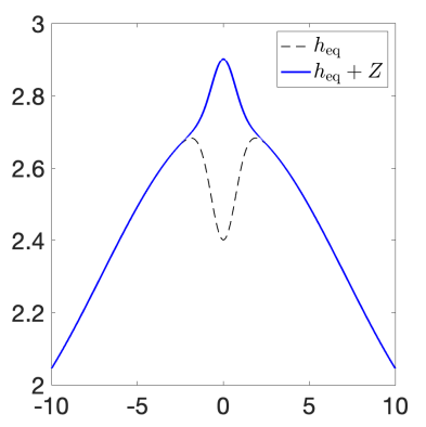
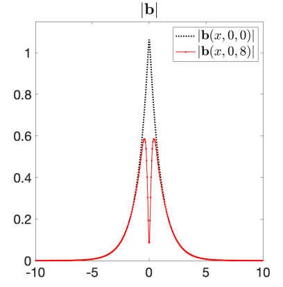
where are computed using (2.17) with . The obtained discrete profile of is plotted in Figure 4.1 (left).

We compute the numerical solutions on a uniform mesh with by the WB and NWB schemes until the final time . The results reported in Table 4.1, show that the WB scheme, as expected, preserves the steady state within the machine accuracy, while the NWB scheme fails to do so.
| Scheme | ||||
|---|---|---|---|---|
| WB | 1.33e-15 | 3.22e-15 | 7.55e-15 | 4.44e-15 |
| NWB | 2.18e-03 | 1.86e-03 | 1.40e-03 | 3.97e-03 |
Next, we examine the ability of the proposed WB scheme to correctly capture the evolution of a small perturbation of the studied steady state. This is done by perturbing the discrete equilibrium fluid depth. Namely, we take the following initial data for :
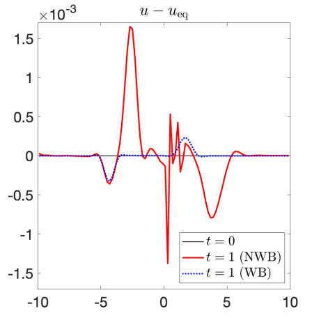
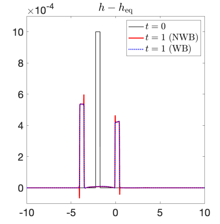
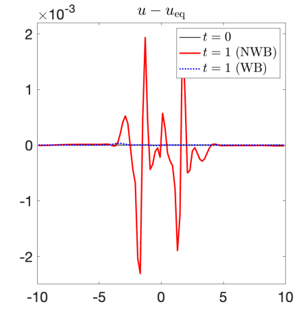
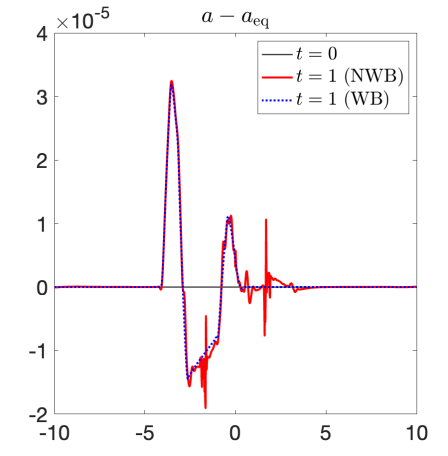
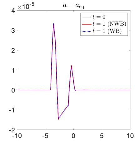
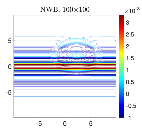
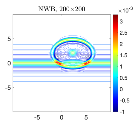
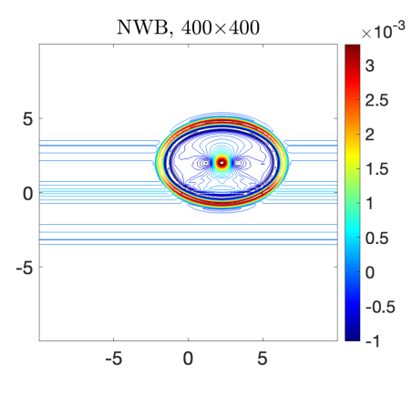
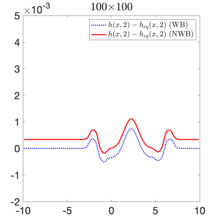
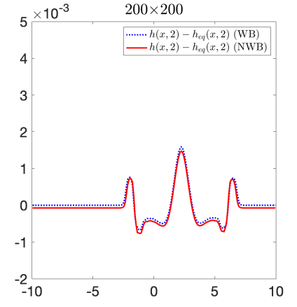
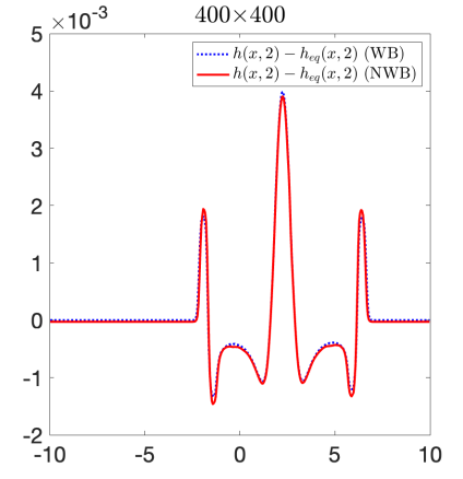
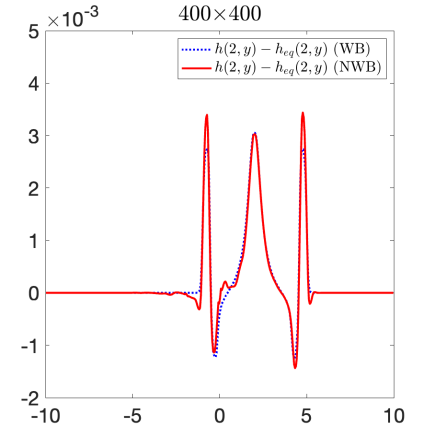
We compute the numerical solutions by both the WB and NWB schemes until the final time on a sequence of meshes with , 1000, and 10000 cells. The obtained differences are plotted in Figure 4.2, where one can see that the NWB scheme fails to capture the correct solution on a coarse mesh with and even when the mesh is refined the NWB solution contains visible oscillations. At the same time, the WB solution is oscillation-free, even on a coarse mesh.
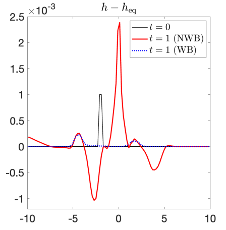
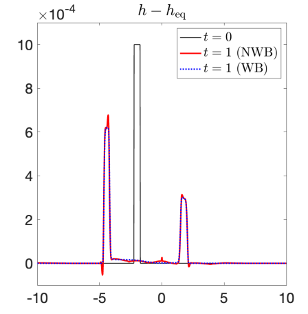
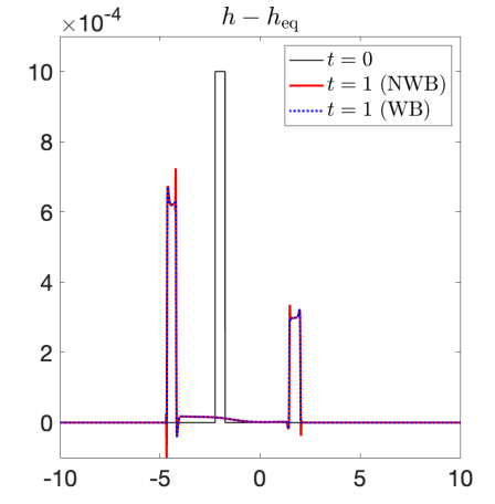
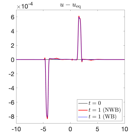
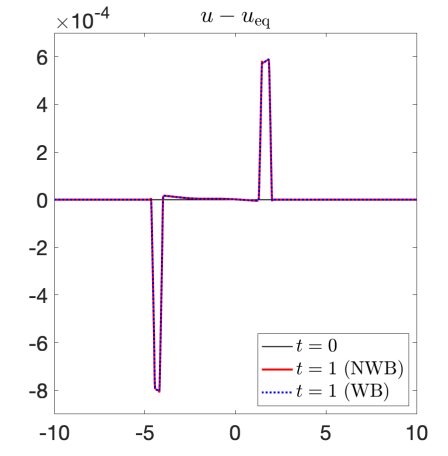
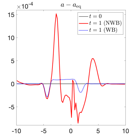
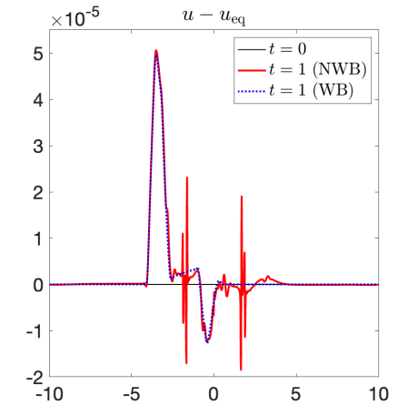
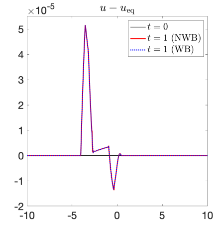
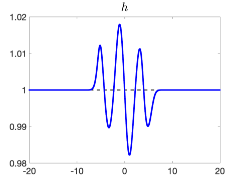
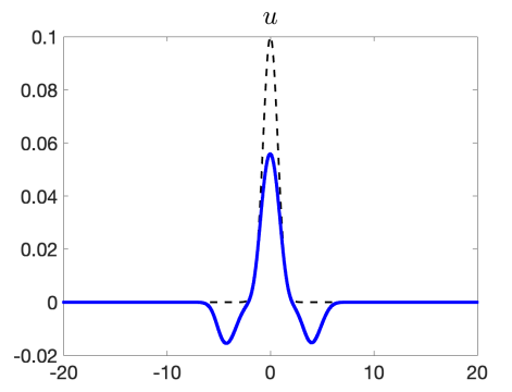
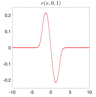
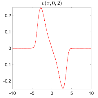
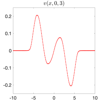
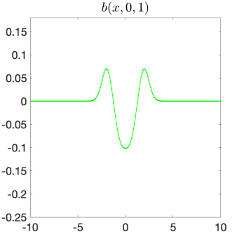
It is also instructive to see the computed differences and ; see Figure 4.3. They clearly show that the initial perturbation results in two wave packets propagating to the right and the left of its location. The phase relations between and in these waves (same phase for the left-moving, and opposite phases for the right-moving waves) match the corresponding phase relations of linear waves on the background of the magnetic field, which can be straightforwardly deduced from the linearized equations (see [79]) with the linearization being justified by the smallness of the perturbation. We also see that, unlike the NWB scheme, the WB one captures the waves properly, even at the lowest resolution.
Example 2—Steady-State with Linear Coriolis Parameter
In the second example, we demonstrate that the proposed 1-D method exactly preserves moving-water equilibria in the so-called equatorial beta-plane approximation of the Coriolis parameter . (The axis of rotation is parallel to the tangent plane at the equator; thus, the constant part of is identically zero.) To this end, we use the following initial conditions that satisfy (2.7), (2.10):
and the bottom topography . The computational domain is and the discrete profile of , which is plotted in Figure 4.1 (right), is obtained precisely as in Example 1 by solving the cubic equation (4.4).
We compute the numerical solutions on a uniform mesh with by the WB and NWB schemes until the final time . The results reported in Table 4.2, show that the WB scheme, as expected, preserves the steady state within the machine accuracy, while the NWB scheme fails to do so.
| Scheme | ||||
|---|---|---|---|---|
| WB | 1.33e-15 | 2.11e-15 | 1.08e-15 | 1.55e-15 |
| NWB | 1.71e-03 | 1.79e-03 | 4.81e-03 | 1.36e-03 |
Next, we examine the ability of the proposed WB scheme to capture a small perturbation of the studied steady state accurately. We use precisely the same perturbed initial as in Example 1 and compute the numerical solutions by both the WB and NWB schemes until the final time on a sequence of meshes with , 1000, and 10000 cells. The obtained differences , , and are plotted in Figure 4.4, where one can see that the NWB scheme fails to capture the correct solution on a coarse mesh with and even when , the NWB solution is still very oscillatory. At the same time, the WB solutions are oscillation-free. Notice that finding linear wave solutions with the meridional (poloidal) magnetic field and with is a nontrivial task, so we do not have here readily available theoretical predictions of the properties of such waves.

Example 3—Magneto-Geostrophic Adjustment at Low Rossby Numbers
In this example, we consider the magneto-geostrophic adjustment problem with low Rossby numbers, that is, with both and . As a result, smooth outward-moving waves are initially not expected to form shocks as they propagate.
We consider the following initial conditions:
with the constant Coriolis parameter and flat bottom topography on the computational domain subject to the outflow boundary conditions.
We first use the above setting to test the experimental rate of convergence achieved by the proposed 1-D flux globalization based WB PCCU scheme. To this end, we compute the solution until on a uniform mesh with and plot the obtained , , , and in Figure 4.5. In order to obtain the experimental rate of convergence, we compute the solution on several different meshes and then use the Runge formula
where denotes the water depth computed on the uniform mesh consisting of cells (similar formulae can be written for the other components of the computed solution). The obtained results, reported in Table 4.3, confirm that the expected second order of accuracy has been reached.

| Rate | Rate | Rate | Rate | |||||
|---|---|---|---|---|---|---|---|---|
| 4000 | 1.26e-03 | 2.19 | 1.69e-03 | 1.93 | 1.10e-03 | 1.86 | 1.70e-03 | 2.34 |
| 8000 | 2.74e-04 | 2.21 | 3.84e-04 | 2.14 | 2.57e-04 | 2.09 | 2.59e-04 | 2.71 |
| 16000 | 6.21e-05 | 2.14 | 7.38e-05 | 2.38 | 6.11e-05 | 2.07 | 4.43e-05 | 2.55 |
| 32000 | 1.49e-05 | 2.06 | 1.38e-05 | 2.42 | 1.50e-05 | 2.02 | 7.23e-06 | 2.62 |
| 64000 | 3.67e-06 | 2.02 | 2.79e-06 | 2.30 | 3.72e-06 | 2.01 | 1.30e-06 | 2.48 |
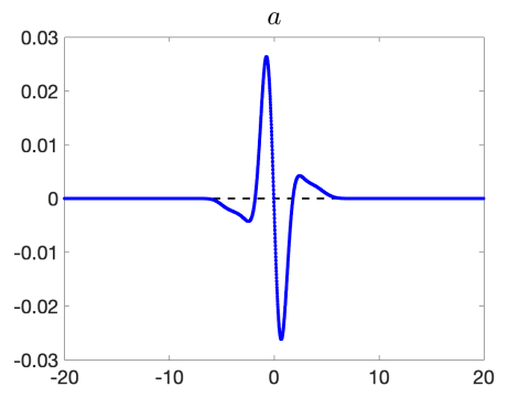
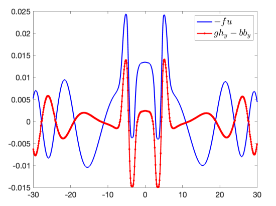
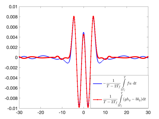
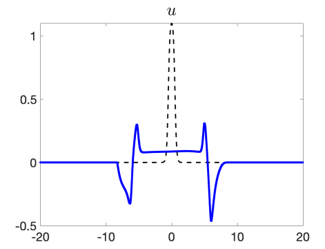
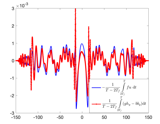
We should emphasize that Figure 4.5 confirms the scenario of magneto-geostrophic adjustment sketched in §4.1.1, showing that at fast magneto-inertia-gravity waves have already been evacuated from the perturbation location and slow Alfvén waves are being emitted, as follows from the phase relations between and , which were already discussed in Example 1. We now test the magneto-geostrophic equilibrium of the quasi-stationary central part of the perturbation. To this end, we compute the numerical solution until a relatively large final time and measure the quantities on both sides of (4.3) as they are to be the same at the aforementioned steady state. However, at , these quantities remain quite different, as shown in Figure 4.6 (left). This often occurs in geostrophic adjustments when waves have near-zero group velocities and thus stay in the center of the computational domain for long times; see, e.g., the discussion in [44]. Under such circumstances, the magneto-geostrophic balance should be checked for time-averaged components. We therefore take the time averages in (4.3),
| (4.5) |
where , and measure the LHS and RHS of (4.5) at . The obtained results are reported in Figure 4.6 (right), where one can see that the proposed method does indeed time-advance the numerical solution to the expected magneto-geostrophic equilibrium.
Example 4—Magneto-Geostrophic Adjustment at High Rossby Numbers
We continue our exploration of magneto-geostrophic adjustment with an example where and . The results are to be compared with those in “pure”, non-magnetic RSW model [6], this is why the initial conditions are the same, in what concerns velocity and thickness, with a superimposed constant meridional magnetic field:
with the constant Coriolis parameter and flat bottom topography on the computational domain subject to the outflow boundary conditions.
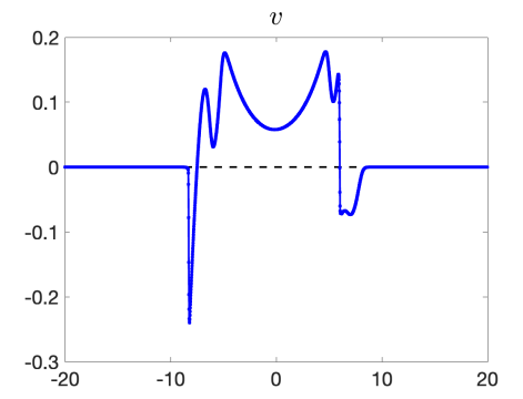
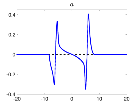
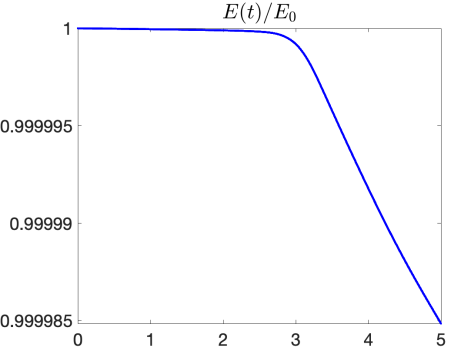
We first compute the solution by the proposed 1-D flux globalization based WB PCCU scheme until on a uniform mesh with . The obtained , , , and are shown in Figure 4.7, where one can clearly see that by that time, compared with the previous example, the solution has developed left- and right-propagating discontinuities. Shock formation is expected, in the light of the results in [6], in the and fields, although the form of both signals differs from those in [6, Figure 2]. So, the evolution of these fields is affected by the mean magnetic field. Moreover, the discontinuities are also clearly seen in the and fields. These contact/tangential discontinuities, which are transverse to the direction of propagation, are well-known in MHD; see, e.g., [51]. A difference, more clearly seen in the left-moving waves, between the speed of the discontinuities observed in the and fields compared with the and ones is since they are associated with faster magneto-inertia-gravity and slower rotation-modified Alfvén waves, respectively. Wave-breaking and shock formation also manifest themselves in the evolution of the total energy (4.1) presented in Figure 4.8, where one can see that the energy first remains practically constant but then diminishes after the appearance of the discontinuity. We have also verified that the energy drops across the shock, as it should.

Similarly to the experiments conducted in the previous example, we then study the convergence towards the magneto-geostrophic equilibrium. To this end, we use the time-averaged computation (see (4.5)) to verify whether the magneto-geostrophic balance has been achieved by (we take a larger final time than in Example 3 as the solution here is nonsmooth and its magnetic field is stronger, so the convergence is expected to be slower). The obtained results are reported in Figure 4.9, where we plot the LHS and RHS of (4.5). One can observe a reasonable agreement, although there is a discrepancy in the center of the original jet, presumably due to nonlinear effects.
4.2 2-D Numerical Examples
4.2.1 General Facts About the 2-D MRSW Model
A straightforward linearization of the system (1.1) over the state of rest with a constant magnetic field reveals the presence of fast magneto-inertia-gravity waves and slow rotation-modified Alfvén waves. The former can propagate in any direction, while the latter propagates only along the direction defined by the magnetic field vector.
We note that, in general, neither geostrophic,
nor magneto-geostrophic,
equilibria are steady solutions of the 2-D MRSW model unless the former one is unidirectional, like in §4.1.1. This situation is analogous to that of non-magnetic RSW equations, for which numerous studies show that, at least at low Rossby numbers, any localized perturbation rapidly adjusts to a state close to geostrophic equilibrium, which then slowly evolves, obeying the so-called quasi-geostrophic dynamics, which is, essentially, vortex dynamics; see, e.g., [78] and references therein. Magneto quasi-geostrophic (MQG) approximation of the MRSW equations, which can be constructed at small Rossby and magnetic Rossby numbers [50, 77], describes slow rotation-modified Alfvén waves together with vortices. Magneto-geostrophic adjustment remains largely unstudied in the 2-D MRSW model; the only work in this direction, to the best of our knowledge, is an investigation in [56] of the evolution of a strong small-scale non-equilibrated Gaussian vortex in a uniform magnetic field.
We should emphasize that an advantage of the 2-D MRSW model compared to the 1-D one is that it allows describing such physically important dynamical entities as vortices. The simplest idealized vortex configuration is axisymmetric with only azimuthal velocity components. In order to better understand this type of structure, it is useful to rewrite the system (1.1) in polar coordinates and in the nonconservative form:
| (4.6) | ||||
where the polar decomposition of velocity and magnetic fields is used: , , where and are unit vectors in and directions, respectively, and .
We notice that the divergence-free condition expressed by the last equation in (4.6) forbids configurations with a purely radial nonsingular magnetic field. We also notice that axisymmetric magneto-cyclo-geostrophic equilibria between , , , and :
| (4.7) |
with are exact steady-state solutions. Hence, we expect relaxation to one of these equilibria (magneto-cyclo-geostrophic adjustment) for initial configurations close to those described by (4.7). Obviously, magneto-cyclo-geostrophic equilibria exist only on the -plane as the beta-effect destroys axial symmetry.
Example 5—Quasi 1-D Steady-State with Linear Coriolis Parameter ()
In the first 2-D numerical example, we demonstrate the ability of the proposed flux globalization based WB PCCU scheme to preserve a quasi 1-D moving-water steady-state. To this end, we use the following initial conditions that satisfy (3.11)–(3.12):
| (4.8) | ||||||||
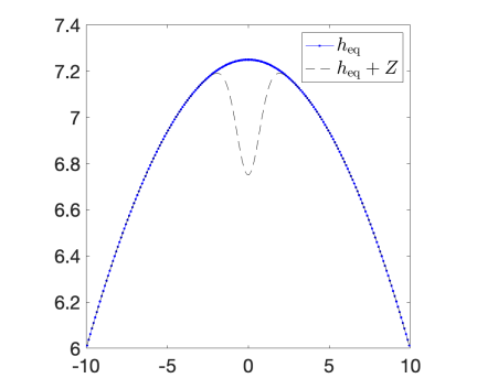
the bottom topography , and the outflow boundary conditions set for the equilibrium variables. Notice that in this example, unlike the 1-D Examples 1 and 2, the profile of , which depends on only, can be computed analytically using (3.11) and (4.8); its 1-D slice is shown in Figure 4.10.
We compute the numerical solutions on the computational domain using a uniform mesh by both the WB and NWB schemes until the final time . The results reported in Table 4.4 show that the WB scheme, as expected, preserves the considered quasi 1-D steady state within the machine accuracy, while the NWB scheme fails to do so.
| Scheme | ||||
|---|---|---|---|---|
| WB | 6.21e-15 | 5.27e-15 | 2.21e-15 | 2.66e-15 |
| NWB | 1.25e-03 | 4.99e-05 | 3.68e-03 | 6.22e-15 |
Next, we examine the ability of the proposed WB scheme to capture a small perturbation of the studied steady state accurately. This is done by perturbing the equilibrium fluid depth, namely, we take the following initial data for :
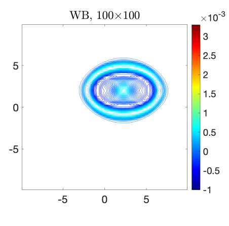
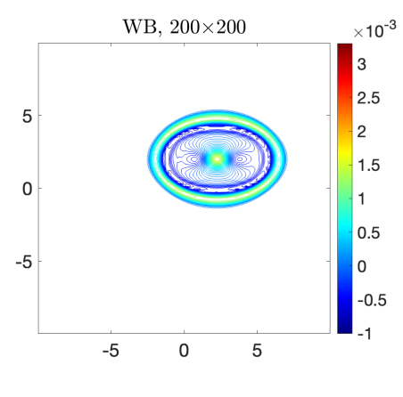
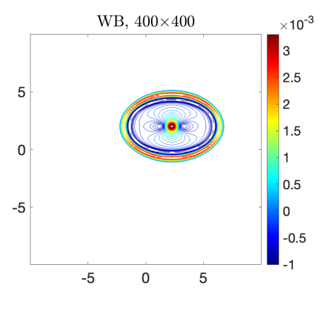
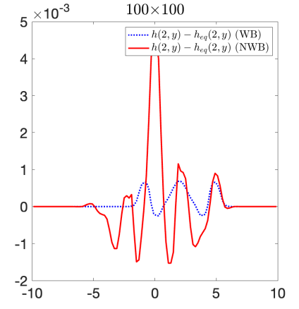
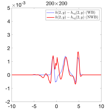
We compute the numerical solutions by both the WB and NWB schemes until the final time on a sequence of , , and uniform meshes. The obtained results () are plotted in Figure 4.11, where one can see that the NWB scheme fails to capture the correct solution on a coarse mesh and even when the mesh is refined the NWB solution contains visible oscillations. At the same time, the WB solution is oscillation-free even when on a coarse mesh. In order to better illustrate the difference between the WB and NWB results, we also plot two 1-D slices and ; see Figure 4.12.
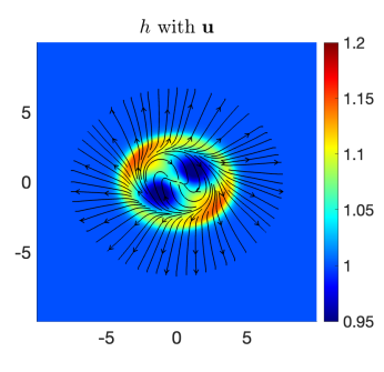
Example 6—Magneto-Cyclo-Geostrophic Adjustment of a Circular Magnetic Anomaly
In this example, we test the process of magneto-cyclo-geostrophic adjustment of an initial configuration with a circular magnetic field only, that is, with a flat and zero velocity. According to the mechanism of magneto-cyclo-geostrophic adjustment explained in §4.2.1, it is expected to evolve towards a vortex in magneto-cyclo-geostrophic equilibrium by emitting outward-traveling inertia-gravity waves. Notice that there are no Alfvén waves that could propagate in this direction.
We consider the following initial conditions:
with the constant Coriolis parameter and flat bottom topography on the computational domain subject to the outflow boundary conditions.
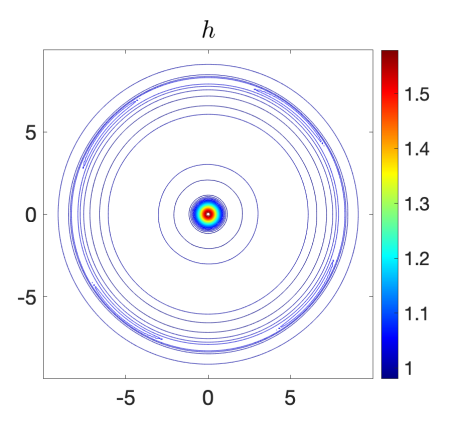
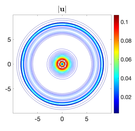
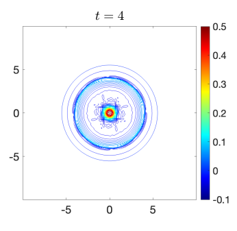
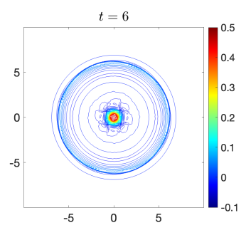
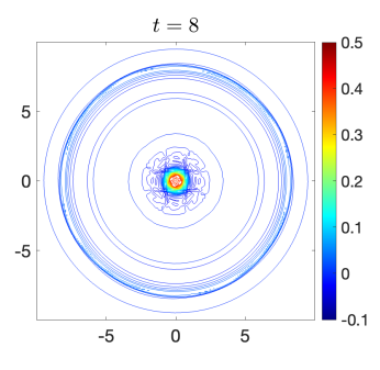
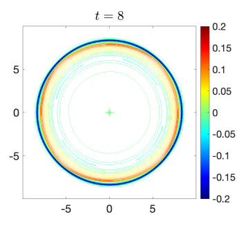
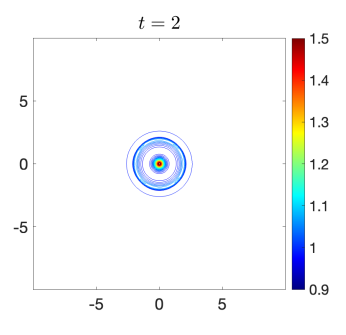
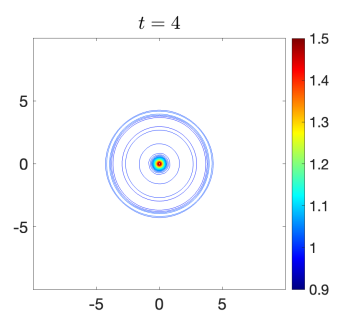
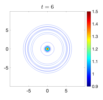
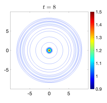
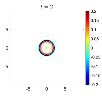
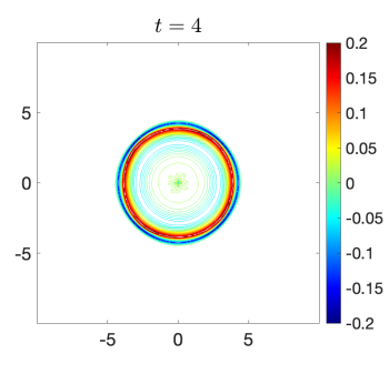
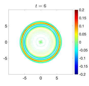
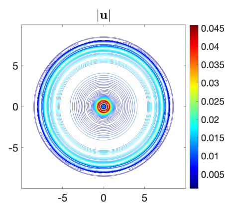
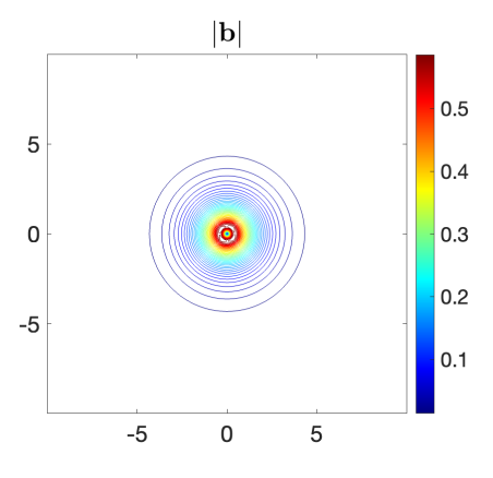
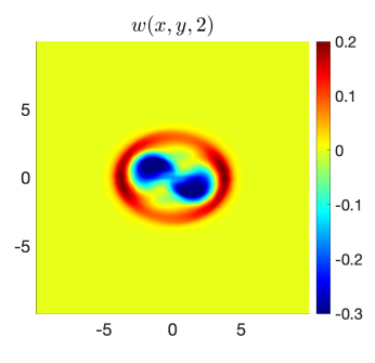
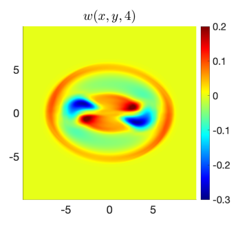
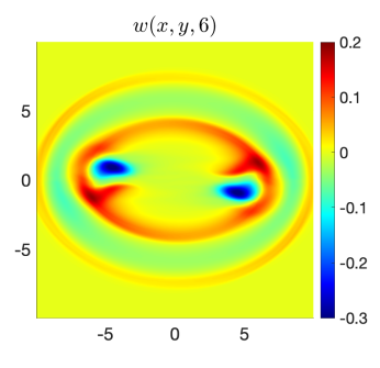
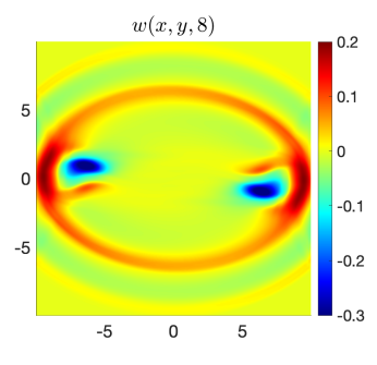
We use the WB scheme to compute the solution until on a uniform mesh and plot the obtained , , and in Figure 4.13, where one can observe the expected structures: a circular wave train of inertia-gravity waves and a central vortex. We also present four-time snapshots at , 4, 6, and 8 of the vorticity and velocity divergence in Figures 4.14 and 4.15, respectively. They confirm the presence of the central vortex and outgoing inertia-gravity waves.


Example 7—Magneto-Cyclo-Geostrophic Adjustment of a Balanced Magnetized Vortex
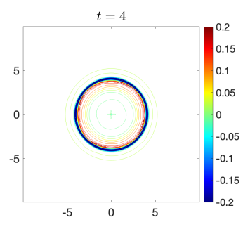
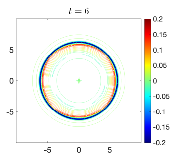
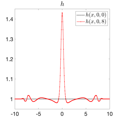
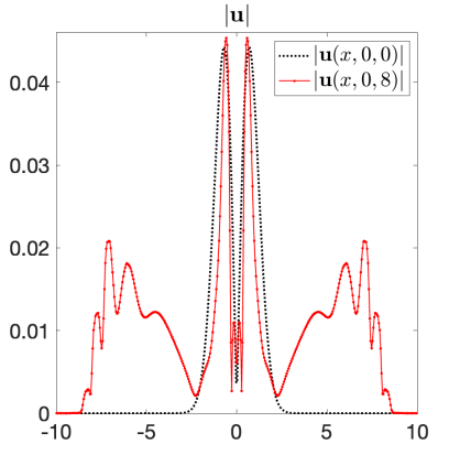
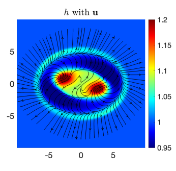
In this example, we continue to test the fundamental process of magneto-cyclo-geostrophic adjustment by adding the effects of topography and exploring the influence of a magnetic field imposed onto an initially balanced vortex. We take a constant Coriolis parameter , a Gaussian-shaped axisymmetric bottom topography , and consider the following initial conditions that correspond to a magnetized balanced vortex:
where the initial velocity magnitude is found by solving the quadratic cyclo-geostrophic balance equation, which reads as
We conduct the computations in the square and set outward boundary conditions at the domain boundaries. We use the WB scheme to compute the solution until the final time on a uniform mesh and plot time snapshots of the obtained fluid level and velocity divergence at , 4, 6, and 8 in Figure 4.16. We also present graphs of and at the final time in Figure 4.17. Like in the preceding magneto-geostrophic adjustment problem (Example 6), one can observe a circular inertia gravity wave train and the remaining central vortex. The 1-D slices , , and at and 8 are displayed in Figure 4.18. They clearly show the evolution towards an equilibrium state verifying (4.7).

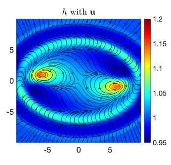
Example 8—Geostrophic Adjustment with Constant Magnetic Field
In the final example, we study how the standard process of (cyclo-) geostrophic adjustment (see [78] and references therein) is influenced by a constant magnetic field, which we chose to be oriented in the -direction. We consider the following initial conditions:
with the constant Coriolis parameter and flat bottom topography on the computational domain subject to the outflow boundary conditions.
We use the WB scheme to compute the solution until the time on a uniform mesh. We show the time snapshots of the fluid depth and vorticity at , 4, 6, and 8 in Figure 4.19, in which we see (i) an elongated in the -direction, consistently with the imposed magnetic field, wave-packet of magneto-inertia-gravity waves; and (ii) two Alfvén wave packets that arise according to the scenario of 1-D adjustment illustrated in Example 3. However, this scenario is modified by 2-D effects, producing vortices linked to the wave packets and, consequently, traveling outward along the -axis. It is worth noting that, as follows from the comparison of the height and vorticity fields at the later stages (third and fourth columns of Figure 4.19), these vortices are in approximate geostrophic equilibrium with negative vorticity corresponding to greater . In order to confirm the origin of the wave packets, we present 1-D slices of and at , 2, 3, and 4 in Figure 4.20, where the characteristic Alfvén-wave signature in these fields can be clearly seen.


5 Conclusion
In this paper, we have developed a novel second-order flux globalization based path-conservative central-upwind (PCCU) scheme for rotating shallow water magnetohydrodynamics equations. Our primary objectives in designing this scheme were twofold: firstly, to maintain the divergence-free constraint of the magnetic field at the discrete level, and secondly, to uphold the well-balanced (WB) property needed to preserve certain physically steady states of the underlying system precisely.
In order to enforce the local divergence-free constraint of the magnetic field, we have considered a Godunov-Powell modified version of the studied system, introduced additional equations through spatial differentiation of the magnetic field equations, and adjusted the reconstruction procedures for magnetic field variables. In order to guarantee the WB property, we have employed a flux globalization technique within the PCCU scheme, enabling the method to maintain both still- and moving-water equilibria.
We have conducted a series of numerical experiments that illustrate the performance of the proposed method. The obtained numerical results demonstrate the scheme’s robustness and showcase its ability to provide high-resolution solutions without the development of spurious oscillations. The presented numerical examples indicate that the scheme accurately captures the details of the fundamental process of magneto-(cyclo-)geostrophic adjustment, resolving equally well the slow motions, shocks, vortices, long Alfvén waves, and the fast wave motions of both kinds—Alfvén and magneto-inertia-gravity—which are present in the system. Thus well-tested, the proposed scheme is ready for in-depth high-resolution numerical studies of the fundamental dynamical processes in the MRSW model, which are important for astro- and geophysical applications. Among them, the influence of the magnetic field on vortex dynamics, which can be highly nontrivial, as shown in recent studies [50, 56] (both were not using dedicated MHD numerical schemes), vortex-Alfvén wave interactions, MHD turbulence, which can be studied in the MRSW model along the lines of similar investigations conducted in the RSW model (see [49]), and so on.
Acknowledgment:
The work of A. Chertock was partially supported by NSF grant DMS-2208438. The work of A. Kurganov was supported in part by NSFC grant 12171226 and by the fund of the Guangdong Provincial Key Laboratory of Computational Science and Material Design (No. 2019B030301001). The work of M. Redle was supported in part by NSF grant DMS-2208438 and by the fund of the DFG Research Unit FOR5409 (grant No. 463312734).
Appendix A Generalized Minmod Piecewise Linear Reconstruction
In this appendix, we provide a brief description of second-order generalized minmod piecewise linear reconstructions (see, e.g., [53, 59, 67]) in both the 1-D and 2-D cases.
In the 1-D case, we consider a function , whose values (either the cell averages or point values) at are available, and approximate the slopes using a generalized minmod limiter to obtain
| (A.1) |
Here, the minmod function is defined by
and the parameter is to be chosen to adjust the amount of numerical dissipation present in the numerical scheme with larger values of leading to sharper but, in general, more oscillatory reconstructions.
We use the slopes computed in (A.1) to obtain the following second-order non-oscillatory piecewise linear reconstruction of :
| (A.2) |
This reconstruction is generically discontinuous at the cell interfaces and hence the one-sided point values of at those points are
| (A.3) |
When a 2-D function is considered, we denote by its discrete values and use the generalized minmod limiter to approximate the - and -slopes:
| (A.4) |
The resulting piecewise linear interpolant then reads as
and the corresponding point values of inside each cell are then given by
Appendix B 1-D Fifth-Order WENO-Z Interpolant
We consider a function , whose point values at are available and explain how to calculate an interpolated left-sided values of at , denoted by . The right-sided value can then be obtained in a mirror-symmetric way.
We construct the three parabolic interpolants , , and on the stencils , , and , respectively, and compute as their weighted average:
where
and the weights are computed by
Here, , , , the smoothness indicators for the corresponding parabolic interpolants are given by
. We have chosen and in all of the numerical examples.
References
- [1] S. Ahmed and S. Zia, The higher-order CESE method for two-dimensional shallow water magnetohydrodynamics equations, Eur. J. Pure Appl. Math., 12 (2019), pp. 1464–1482.
- [2] E. Audusse, V. Dubos, A. Duran, N. Gaveau, Y. Nasseri, and Y. Penel, Numerical approximation of the shallow water equations with Coriolis source term, in CEMRACS 2019—geophysical fluids, gravity flows, vol. 70 of ESAIM Proc. Surveys, EDP Sci., Les Ulis, 2021, pp. 31–44.
- [3] D. S. Balsara and D. S. Spicer, A staggered mesh algorithm using high order Godunov fluxes to ensure solenoidal magnetic fields in magnetohydrodynamic simulations, J. Comput. Phys., 149 (1999), pp. 270–292.
- [4] R. Borges, M. Carmona, B. Costa, and W. S. Don, An improved weighted essentially non-oscillatory scheme for hyperbolic conservation laws, J. Comput. Phys., 227 (2008), pp. 3191–3211.
- [5] F. Bouchut, Efficient numerical finite volume schemes for shallow water models, in Nonlinear Dynamics of Rotating Shallow water: Methods and Advances, V. Zeitlin, ed., vol. 2 of Edited Series on Advances in Nonlinear Science and Complexity, Elsevier, 2007, ch. 4, pp. 189–256.
- [6] F. Bouchut, J. Le Sommer, and V. Zeitlin, Frontal geostrophic adjustment and nonlinear wave phenomena in one-dimensional rotating shallow water. II. High-resolution numerical simulations, J. Fluid Mech., 514 (2004).
- [7] F. Bouchut and X. Lhébrard, A multi well-balanced scheme for the shallow water MHD system with topography, Numer. Math., 136 (2017), pp. 875–905.
- [8] J. U. Brackbill and D. C. Barnes, The effect of nonzero on the numerical solution of the magnetohydrodynamic equations, J. Comput. Phys., 35 (1980), pp. 426–430.
- [9] Y. Cao, A. Kurganov, and Y. Liu, Flux globalization based well-balanced path-conservative central-upwind schemes for the thermal shallow water equations, Commun. Comput. Phys., 34 (2023), pp. 993–1042.
- [10] Y. Cao, A. Kurganov, Y. Liu, and R. Xin, Flux globalization based well-balanced path-conservative central-upwind schemes for shallow water models, J. Sci. Comput., 92 (2022). Paper No. 69, 31 pp.
- [11] Y. Cao, A. Kurganov, Y. Liu, and V. Zeitlin, Flux globalization based well-balanced path-conservative central-upwind scheme for two-layer thermal rotating shallow water equations, J. Comput. Phys., 474 (2023). Paper No. 111790, 29 pp.
- [12] V. Caselles, R. Donat, and G. Haro, Flux-gradient and source-term balancing for certain high resolution shock-capturing schemes, Comput. & Fluids, 38 (2009), pp. 16–36.
- [13] M. Castro, B. Costa, and W. S. Don, High order weighted essentially non-oscillatory WENO-Z schemes for hyperbolic conservation laws, J. Comput. Phys., 230 (2011), pp. 1766–1792.
- [14] M. J. Castro, J. A. López, and C. Parés, Finite volume simulation of the geostrophic adjustment in a rotating shallow-water system, SIAM J. Sci. Comput., 31 (2008), pp. 444–477.
- [15] M. J. Castro Díaz, A. Kurganov, and T. Morales de Luna, Path-conservative central-upwind schemes for nonconservative hyperbolic systems, ESAIM Math. Model. Numer. Anal., 53 (2019), pp. 959–985.
- [16] Y. Cheng, A. Chertock, M. Herty, A. Kurganov, and T. Wu, A new approach for designing moving-water equilibria preserving schemes for the shallow water equations, J. Sci. Comput., 80 (2019), pp. 538–554.
- [17] A. Chertock, M. Dudzinski, A. Kurganov, and M. Lukáčová-Medviďová, Well-balanced schemes for the shallow water equations with Coriolis forces, Numer. Math., 138 (2018), pp. 939–973.
- [18] A. Chertock, M. Herty, and c. N. Özcan, Well-balanced central-upwind schemes for systems of balance laws, in Theory, numerics and applications of hyperbolic problems. I, vol. 236 of Springer Proc. Math. Stat., Springer, Cham, 2018, pp. 345–361.
- [19] A. Chertock, A. Kurganov, M. Redle, and K. Wu, A new locally divergence-free path-conservative central-upwind scheme for ideal and shallow water magnetohydrodynamics. In: ArXiv preprint (2022), arXiv:2212.02682.
- [20] H. De Sterck, Hyperbolic theory of the “shallow water” magnetohydrodynamics equations, Phys. Plasmas, 8 (2001), pp. 3293–3304.
- [21] , Multi-dimensional upwind constrained transport on unstructured grids for “shallow water” magnetohydrodynamics, in Proceedings of the 15th AIAA Computational Fluid Dynamics Conference, AIAA 2001‐-2623, 2001.
- [22] P. J. Dellar, Hamiltonian and symmetric hyperbolic structures of shallow water magnetohydrodynamics, Phys. Plasmas, 9 (2002), pp. 1130–1136.
- [23] V. Desveaux and A. Masset, A fully well-balanced scheme for shallow water equations with Coriolis force, Commun. Math. Sci., 20 (2022), pp. 1875–1900.
- [24] W.-S. Don and R. Borges, Accuracy of the weighted essentially non-oscillatory conservative finite difference schemes, J. Comput. Phys., 250 (2013), pp. 347–372.
- [25] D. Donat and A. Martinez-Gavara, Hybrid second order schemes for scalar balance laws, J. Sci. Comput., 48 (2011), pp. 52–69.
- [26] J. Dong and D. F. Li, Well-balanced nonstaggered central schemes based on hydrostatic reconstruction for the shallow water equations with Coriolis forces and topography, Math. Methods Appl. Sci., 44 (2021), pp. 1358–1376.
- [27] J. Duan and H. Tang, High-order accurate entropy stable finite difference schemes for the shallow water magnetohydrodynamics, J. Comput. Phys., 431 (2021). Paper No. 110136, 26 pp.
- [28] M. Dumbser, D. S. Balsara, M. Tavelli, and F. Fambri, A divergence-free semi-implicit finite volume scheme for ideal, viscous, and resistive magnetohydrodynamics, Internat. J. Numer. Methods Fluids, 89 (2019), pp. 16–42.
- [29] M. A. Fedotova, D. A. Klimachkov, and A. S. Petrosyan, The shallow-water magnetohydrodynamic theory of stratified rotating astrophysical plasma flows: Beta-plane approximation and magnetic Rossby waves, Plasma Phys. Rep., 46 (2020), pp. 50–64.
- [30] P. Fu, F. Li, and Y. Xu, Globally divergence-free discontinuous Galerkin methods for ideal magnetohydrodynamic equations, J. Sci. Comput., 77 (2018), pp. 1621–1659.
- [31] F. G. Fuchs, A. D. McMurry, S. Mishra, N. H. Risebro, and K. Waagan, Approximate Riemann solvers and robust high-order finite volume schemes for multi-dimensional ideal MHD equations, Commun. Comput. Phys., 9 (2011), pp. 324–362.
- [32] L. Gascón and J. M. Corderán, Construction of second-order TVD schemes for nonhomogeneous hyperbolic conservation laws, J. Comput. Phys., 172 (2001), pp. 261–297.
- [33] P. A. Gilman, Magnetohydrodynamic “shallow water” equations for the solar tachocline, Astrophys. J. Lett., 544 (2000), pp. L79–L82.
- [34] S. Gottlieb, D. Ketcheson, and C.-W. Shu, Strong stability preserving Runge-Kutta and multistep time discretizations, World Scientific Publishing Co. Pte. Ltd., Hackensack, NJ, 2011.
- [35] S. Gottlieb, C.-W. Shu, and E. Tadmor, Strong stability-preserving high-order time discretization methods, SIAM Rev., 43 (2001), pp. 89–112.
- [36] C. Helzel, J. A. Rossmanith, and B. Taetz, A high-order unstaggered constrained-transport method for the three-dimensional ideal magnetohydrodynamic equations based on the method of lines, SIAM J. Sci. Comput., 35 (2013), pp. A623–A651.
- [37] P. Janhunen, A positive conservative method for magnetohydrodynamics based on HLL and Roe methods, J. Comput. Phys., 160 (2000), pp. 649–661.
- [38] F. Kemm, Roe-type schemes for shallow water magnetohydrodynamics with hyperbolic divergence cleaning, Appl. Math. Comput., 272 (2016), pp. 385–402.
- [39] F. Kemm, Roe-type schemes for shallow water magnetohydrodynamics with hyperbolic divergence cleaning, Appl. Math. Comput., 272 (2016), pp. 385–402.
- [40] C. Klingenberg, A. Kurganov, Y. Liu, and M. Zenk, Moving-water equilibria preserving HLL-type schemes for the shallow water equations, Commun. Math. Res., 36 (2020), pp. 247–271.
- [41] T. Kröger and M. Lukáčová-Medviďová, An evolution Galerkin scheme for the shallow water magnetohydrodynamic equations in two space dimensions, J. Comput. Phys., 206 (2005), pp. 122–149.
- [42] A. Kurganov and C.-T. Lin, On the reduction of numerical dissipation in central-upwind schemes, Commun. Comput. Phys., 2 (2007), pp. 141–163.
- [43] A. Kurganov, Y. Liu, and R. Xin, Well-balanced path-conservative central-upwind schemes based on flux globalization, J. Comput. Phys., 474 (2023). Paper No.111773, 32 pp.
- [44] A. Kurganov, Y. Liu, and V. Zeitlin, A well-balanced central-upwind scheme for the thermal rotating shallow water equations, J. Comput. Phys., 411 (2020). Paper No. 109414, 24 pp.
- [45] A. Kurganov, S. Noelle, and G. Petrova, Semidiscrete central-upwind schemes for hyperbolic conservation laws and Hamilton-Jacobi equations, SIAM J. Sci. Comput., 23 (2001), pp. 707–740.
- [46] A. Kurganov, M. Prugger, and T. Wu, Second-order fully discrete central-upwind scheme for two-dimensional hyperbolic systems of conservation laws, SIAM J. Sci. Comput., 39 (2017), pp. A947–A965.
- [47] A. Kurganov and E. Tadmor, New high-resolution central schemes for nonlinear conservation laws and convection-diffusion equations, J. Comput. Phys., 160 (2000), pp. 241–282.
- [48] A. Kurganov and E. Tadmor, Solution of two-dimensional Riemann problems for gas dynamics without Riemann problem solvers, Numer. Methods Partial Differential Equations, 18 (2002), pp. 584–608.
- [49] N. Lahaye and V. Zeitlin, Decaying vortex and wave turbulence in rotating shallow water model, as follows from high resolution direct numerical simulations, Phys. Fluids, 24 (2012). Paper No. 115106, 14 pp.
- [50] , Coherent magnetic modon solutions in quasi-geostrophic shallow water magnetohydrodynamics, J. Fluid Mech., 941 (2022). Paper No. A15, 22 pp.
- [51] L. D. Landau and E. M. Lifshitz, Course of theoretical physics. Vol. 8, Pergamon International Library of Science, Technology, Engineering and Social Studies, Pergamon Press, Oxford, 1984. Electrodynamics of continuous media, Translated from the second Russian edition by J. B. Sykes, J. S. Bell and M. J. Kearsley, Second Russian edition revised by Lifshits and L. P. Pitaevskiĭ.
- [52] F. Li and C.-W. Shu, Locally divergence-free discontinuous Galerkin methods for MHD equations, J. Sci. Comput., 22/23 (2005), pp. 413–442.
- [53] K.-A. Lie and S. Noelle, On the artificial compression method for second-order nonoscillatory central difference schemes for systems of conservation laws, SIAM J. Sci. Comput., 24 (2003), pp. 1157–1174.
- [54] P. Londrillo and L. Del Zanna, On the divergence-free condition in Godunov-type schemes for ideal magnetohydrodynamics: the upwind constrained transport method, J. Comput. Phys., 195 (2004), pp. 17–48.
- [55] M. Lukáčová-Medviďová, S. Noelle, and M. Kraft, Well-balanced finite volume evolution Galerkin methods for the shallow water equations, J. Comput. Phys., 221 (2007), pp. 122–147.
- [56] M. Magill, A. Coutino, B. A. Storer, M. Stastna, and F. G. Poulin, Dynamics of nonlinear Alfvén waves in the shallow water magnetohydrodynamic equations, Phys. Rev. Fluids, 4 (2019). Paper No. 053701, 22 pp.
- [57] A. Martinez-Gavara and R. Donat, A hybrid second order scheme for shallow water flows, J. Sci. Comput., 48 (2011), pp. 241–257.
- [58] S. Mishra and E. Tadmor, Constraint preserving schemes using potential-based fluxes. III. Genuinely multi-dimensional schemes for MHD equations, ESAIM Math. Model. Numer. Anal., 46 (2012), pp. 661–680.
- [59] H. Nessyahu and E. Tadmor, Nonoscillatory central differencing for hyperbolic conservation laws, J. Comput. Phys., 87 (1990), pp. 408–463.
- [60] A. Petrosyan, D. Klimachkov, M. Fedotova, and T. Zinyakov, Shallow water magnetohydrodynamics in plasma astrophysics. Waves, turbulence, and zonal flows, Atmosphere, 11 (2020). Paper No. 314, 16 pp.
- [61] K. G. Powell, P. L. Roe, T. J. Linde, T. I. Gombosi, and D. L. De Zeeuw, A solution-adaptive upwind scheme for ideal magnetohydrodynamics, J. Comput. Phys., 154 (1999), pp. 284–309.
- [62] K. G. Powell, P. L. Roe, R. S. Myong, T. Gombosi, and D. De Zeeuw, An upwind scheme for magnetohydrodynamics, in 12th Computational Fluid Dynamics Conference: AIAA Paper 95-1704-CP, 1995, pp. 661–674.
- [63] S. Qamar and S. Mudasser, A kinetic flux-vector splitting method for the shallow water magnetohydrodynamics, Comput. Phys. Comm., 181 (2010), pp. 1109–1122.
- [64] S. Qamar and G. Warnecke, Application of space-time CE/SE method to shallow water magnetohydrodynamic equations, J. Comput. Appl. Math., 196 (2006), pp. 132–149.
- [65] B. Raphaldini and C. F. M. Raupp, Nonlinear MHD Rossby wave interactions and persistent geomagnetic field structures, Proc. A., 476 (2020). Paper No. 20200174, 20 pp.
- [66] J. A. Rossmanith, A wave propagation method with constrained transport for ideal and shallow water magnetohydrodynamics, ProQuest LLC, Ann Arbor, MI, 2002. Thesis (Ph.D.)–University of Washington.
- [67] P. K. Sweby, High resolution schemes using flux limiters for hyperbolic conservation laws, SIAM J. Numer. Anal., 21 (1984), pp. 995–1011.
- [68] S. Tobias, P. Diamond, and D. Hughes, Beta-plane magnetohydrodynamic turbulence in the solar tachocline, Astrophys. J. Lett., 667 (2007), pp. L113–L116.
- [69] G. Tóth, The constraint in shock-capturing magnetohydrodynamics codes, J. Comput. Phys., 161 (2000), pp. 605–652.
- [70] R. Touma, Unstaggered central schemes with constrained transport treatment for ideal and shallow water magnetohydrodynamics, Appl. Numer. Math., 60 (2010), pp. 752–766.
- [71] K. Waagan, C. Federrath, and C. Klingenberg, A robust numerical scheme for highly compressible magnetohydrodynamics: Nonlinear stability, implementation and tests, J. Comput. Phys., 230 (2011), pp. 3331–3351.
- [72] A. R. Winters and G. J. Gassner, An entropy stable finite volume scheme for the equations of shallow water magnetohydrodynamics, J. Sci. Comput., 67 (2016), pp. 514–539.
- [73] K. Wu and C.-W. Shu, A provably positive discontinuous Galerkin method for multidimensional ideal magnetohydrodynamics, SIAM J. Sci. Comput., 40 (2018), pp. B1302–B1329.
- [74] K. Wu and C.-W. Shu, Geometric Quasilinearization Framework for Analysis and Design of Bound-Preserving Schemes, SIAM Rev., 65 (2023), pp. 1031–1073.
- [75] Z. Xu, D. S. Balsara, and H. Du, Divergence-free WENO reconstruction-based finite volume scheme for solving ideal MHD equations on triangular meshes, Commun. Comput. Phys., 19 (2016), pp. 841–880.
- [76] T. Zaqarashvili, V, M. Albekioni, J. L. Ballester, Y. Bekki, L. Biancofiore, A. C. Birch, M. Dikpati, L. Gizon, E. Gurgenashvili, E. Heifetz, A. F. Lanza, S. W. McIntosh, L. Ofman, R. Oliver, B. Proxauf, O. M. Umurhan, and R. Yellin-Bergovoy, Rossby waves in astrophysics, Space Sci. Rev., 217 (2021), pp. 1–93.
- [77] V. Zeitlin, Remarks on rotating shallow-water magnetohydrodynamics, Nonlinear Process. Geophys., 20 (2013), pp. 893–898.
- [78] V. Zeitlin, Geophysical fluid dynamics: understanding (almost) everything with rotating shallow water models, Oxford University Press, 2018.
- [79] V. Zeitlin, C. Lusso, and F. Bouchut, Geostrophic vs magneto-geostrophic adjustment and nonlinear magneto-inertia-gravity waves in rotating shallow water magnetohydrodynamics, Geophys. Astrophys. Fluid Dyn., 109 (2015), pp. 497–523.
- [80] V. Zeitlin, S. B. Medvedev, and R. Plougonven, Frontal geostrophic adjustment, slow manifold and nonlinear wave phenomena in one-dimensional rotating shallow water. I. Theory, J. Fluid Mech., 481 (2003), pp. 269–290.
- [81] S. Zia, M. Ahmed, and S. Qamar, Numerical solution of shallow water magnetohydrodynamic equations with non-flat bottom topography, Int. J. Comput. Fluid Dyn., 28 (2014), pp. 56–75.