Efficient Point Cloud Registration using Dynamic Networks

Abstract

For the point cloud registration task, a significant challenge arises from non-overlapping points that consume extensive computational resources while negatively affecting registration accuracy. In this paper, we introduce a dynamic approach, widely utilized to improve network efficiency in computer vision tasks, to the point cloud registration task. We employ an iterative registration process on point cloud data multiple times to identify regions where matching points cluster, ultimately enabling us to remove noisy points. Specifically, we begin with deep global sampling to perform coarse global registration. Subsequently, we employ the proposed refined node proposal module to further narrow down the registration region and perform local registration. Furthermore, we utilize a spatial consistency-based classifier to evaluate the results of each registration stage. The model terminates once it reaches sufficient confidence, avoiding unnecessary computations. Extended experiments demonstrate that our model significantly reduces time consumption compared to other methods with similar results, achieving a speed improvement of over $41\%$ on indoor dataset (3DMatch) and $33\%$ on outdoor datasets (KITTI) while maintaining competitive registration recall requirements.

1 Introduction

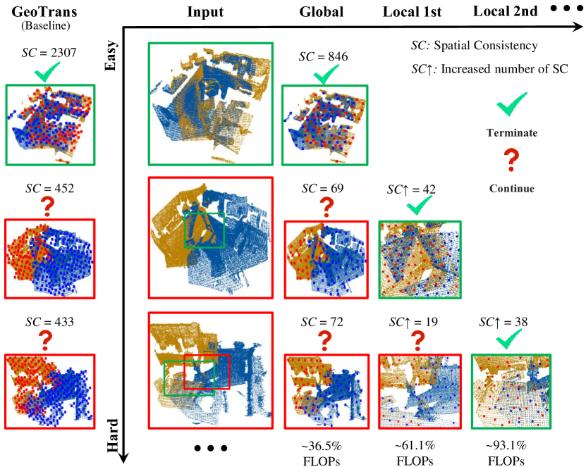
Figure 1: Our method samples sparser point clouds for registration in the global stage and iteratively discovers overlapping regions in the local stage. “FLOPs” refers to the proportion of the computation required by our method versus processing by GeoTrans [39].

Point cloud registration (PCR) aims to estimate the 3D transformation required to align a pair of point clouds, which is an important research topic in various 3D visual applications, including 3D reconstruction [47], autonomous driving [64], robotics [32], etc. In traditional methods [33, 13, 41], hand-crafted descriptors often fall short of accurately capturing the unique point cloud features, resulting in a significant amount of time and computational resources spent on eliminating incorrect correspondences and exhibiting a significant decrease in stability and accuracy.

With the recent advancements in deep learning, many researchers use learning-based approaches to extract the features of the point cloud and employ cross-attention mechanisms to point cloud pairs to facilitate learning of similar features. For instance, Geotransformer [39] introduces a geometric transformer to learn robust features. However, due to the often substantial volume of real-world data in practical scenarios, learning-based methods for point cloud registration tend to exhibit high time complexity and add additional computational overhead. Currently, to address this problem, existing methods employ a downsampling network (e.g., PointNet [38], KPConv [48]) that selects points from dense points clouds through multiple hierarchical levels to obtain a sparse point set and corresponding point-wise features by applying convolutions at each level. Then, the point set of the deepest layer is passed to the encoder module to enable information interaction. This downsampling is often performed globally. However, there are often point clouds with partial overlap, which may lead to many outliers (points outside the overlapping region) which can interfere with the subsequent calculations for point feature pairing and unnecessarily consume a significant amount of computational resources.

Starting from this observation, we introduce the concept of the dynamic network into point cloud registration tasks. Dynamic networks are a type of network model that dynamically adjusts its structure based on input data and computational resources during inference. We adapt the spatial-wise dynamic network to propose improvements for addressing spatial redundancy in point cloud registration tasks. Previously, dynamic network methods were primarily applied to 2D visual tasks, while for 3D point clouds, the irregularity and larger scale of the data make managing spatial redundancy more challenging than in the case of images. To address this challenge, drawing inspiration from GFNet [52], we perform global sampling during the global stage to obtain a reduced number of sample points for global registration. Subsequently, during the local registration stage, we gradually narrowed down the scope of global registration, iteratively searching for regions within the inlier set for fine-grained registration. Compared with existing registration methods, our approach significantly reduces the computational cost of feature encoding due to the dynamic network using fewer point clouds for registration.

Our proposed network primarily consists of two stages. Firstly, in the global registration stage, we employ global sampling for candidate pair selection and conduct coarse registration using a sparser input. In practice, we observe that a large portion of scenes with discriminative features can easily be correctly aligned with high accuracy and plenty of pairings in the global registration stage. When the global registration fails to produce sufficient correspondences, our network searches for regions where paired points are clustered together to proceed with the next registration. Specifically, in the local registration stage, we perform density-based clustering on the paired points from global registration. Based on the clustering results, we select regions within the inlier set and calculate cluster centers to be used in the following local registration stage. After each registration stage, we use a classifier to evaluate the results of the current registration and decide whether to proceed with the next registration stage. We iterate the local registration stage until the termination condition is satisfied.

To the best of our knowledge, we are the first to introduce the dynamic network to improve the efficiency of point cloud registration, which is different from other point cloud dynamic networks [31, 26]. Our key contributions are as follows:

• We propose a novel registration network to dynamically discover the overlapping regions between point clouds, which effectively removes outliers and facilitates adaptive inference in the testing phase.

• We develop a refined node proposal module by using the DBSCAN algorithm to narrow down the point cloud registration region, efficiently reducing the computational load without introducing additional networks.

• We significantly reduce point cloud registration time by over $41\%$ on indoor dataset (3DMatch) and $33\%$ on outdoor datasets (KITTI) while maintaining competitive registration accuracy in a more efficient registration method.

2 Related Work

Correspondence-based Methods.

Traditional methods extract correspondences between two point clouds based on feature descriptors and then calculate the transformation based on RANSAC [19]. Recently, many variants [20, 5, 56] propose using outlier removal to improve the accuracy of correspondences. DGR [12] and 3DRegNet [37] consider the inlier/outlier determination as a classification problem. PointDSC [4] and SC²-PCR [9, 10] proposes the outlier rejection module by introducing deep spatial consistency and global consistency to measure the similarity between correspondences. Recently, MAC [66] developed a compatibility graph to render the affinity relationship between correspondences and construct the maximal cliques to represent consensus sets. Although these methods have made significant progress, they are all greatly affected by initial correspondence. In Comparison, our work insights by the idea of the dynamic network to iteratively select matching points based on the global pairing relationship and further optimize the feature of points during iteration to improve the accuracy of correspondences.

Deep-learned Feature Descriptors.

The feature descriptor in the point cloud registration process is used to extract features to construct correspondences between similar point clouds. Compared with traditional hand-crafted descriptors such as [33, 41, 13, 42], descriptors based on deep learning have developed rapidly in recent years. As a pioneer, 3DMatch [65] learns 3D geometric features to convert local patches into voxel representations. Later, PointNetLK [3] and PCRNet [45] integrate PointNet [38] into the point registration task and other deep learning methods [14, 8, 58, 1, 15] improve feature extraction module to enhances the capability of feature descriptors. However, these methods are greatly affected by the overlap rate. Recently, more and more works [59, 67, 61, 51] focus on the low overlap problems. Predator [30] extracts low-overlap point clouds dataset from 3DMatch to form 3DLoMatch and uses the cross-attention module to interact with the point clouds to build feature descriptors. CoFiNet [60] leverages a two-stage method, using down-sampling and similarity matrices for rough matching and up-sampling the paired point neighborhood to obtain fine matching. GeoTransformer [39] learns more geometric structure features to improve the robustness of PCR and achieves high accuracy. Additionally, RoITr [63] addresses rotation-invariant problems by introducing novel local attention mechanisms and global rotation-invariant transformers. These methods compute features for each point and its neighborhood, resulting in an unavoidably large amount of computation. BUFFER [2] attempts to improve the computation efficiency and accuracy of PCR, but its performance is mainly reflected in its generalization ability. Our method uses sparser sampling in the down-sampling stage to compute global feature descriptors, reducing the consumption of computational resources in the registration process.

Dynamic Neural Networks.

The dynamic neural network is a structure that dynamically changes based on computational resources and input data. Compared to static networks with fixed parameters and computational graphs at the inference stage, dynamic networks can adapt their parameters or structures to different inputs, leading to notable advantages in terms of accuracy, computational efficiency, adaptiveness, etc [23]. In recent years, many advanced dynamic network works have been proposed and mainly divided into three different aspects: 1) sample-wise dynamic networks [29, 49, 35, 25, 54] are designed to adjust network architectures and network parameters to reduce computation while maximizing representation power; 2) temporal-wise dynamic networks [36, 46, 18, 57, 22, 53] treat video data as a sequence of images and adaptively save computation at specific time steps or sampled frames along temporal dimension; 3) spatial-wise dynamic networks [68, 16, 40, 6, 28, 50] process different spatial locations with different computation and exploit spatial redundancy to improve efficiency. Our approach is mainly related to spatial-wise methods. DRConv [7] designs a binary mask for convolution block to reduce the number of image pixel calculations. Mobilenet [27, 43] observes that a low resolution might be sufficient for most ”easy” samples and exploits feature solutions to remove redundancy. Besides, early-exiting mechanism [34, 24, 62] is widely studied and used to decide whether the network continues. GFNet [52] imitates the visual system of the human eye and processes an observation process from a global glance to a local focus to search more critical regions. Based on GFNet, we propose a coarse-to-fine feature learning approach combined with registration evaluation to adjust the registration range.

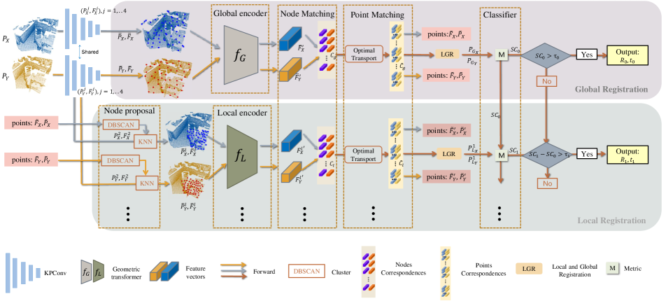
Figure 2: Overview. Our method iteratively discovers overlapping regions, mainly divided into two parts: global registration and local registration. We first perform a multi-level downsample and extract the initial feature by the KPConv backbone. Then, we pass the coarse node into global registration to match the global point cloud to obtain the pairing points $\tilde{P}_{X}$ and $\tilde{P}_{Y}$. Next, the node proposal module in the local registration stage cluster the paired points of the global registration and obtain the new coarse node for local registration again. After each registration step finishes, a classifier is used to determine whether the current result requires further iteration.

3 Method

Given a pair of 3D point clouds $P_{X}=\{p_{x_{i}}\in\mathbb{R}^{3}\,|\,i=1,\ldots,N\}$ and $P_{Y}=\{p_{y_{i}}\in\mathbb{R}^{3}\,|\,i=1,\ldots,M\}$, the purpose of our task is to estimate a rigid transformation $SE(3)$ which aligns the point clouds X and Y with a rotation matrix $R\in SO(3)$ and a translation $T\in\mathbb{R}^{3}$. Fig. 2 shows our overview framework. Similar to  [30, 60], we first adopt the backbone, KPConv [48], to perform multi-scale sampling on the input point clouds and extract initial features of each point (Sec.3.1). Then, our method is divided into two parts, namely the global registration stage and the local registration stage. In the global stage, registration is used to conduct coarse-grained registration of the data (Sec.3.2). On this basis, the classifier is used to judge whether the results meet the accuracy requirements (Sec.3.4). For complex scenes, we use the results of global registration to further perform local registration (Sec.3.3).

3.1 Multi-level Sampling and Feature Extraction

Before global registration, we first perform uniform downsampling in the original input data. Inspired by GFNet [52], we observe that in point cloud registration tasks, full data may not always be necessary for computations and that only partially accurate pairing relationships can yield satisfactory results. In the global registration stage, we use a minimal number of data points to create a global representation of the point cloud for global registration, reserving more computational resources for the subsequent local registration phase. We utilize the KPConv network [48] for multi-level downsampling, obtaining multiple levels of points $P_{X}^{j}\in\mathbb{R}^{N_{j}*3}$,$P_{Y}^{j}\in\mathbb{R}^{M_{j}*3}$ and their corresponding features $F_{X}^{j}\in\mathbb{R}^{N_{j}*D}$,$F_{Y}^{j}\in\mathbb{R}^{M_{j}*D}$ ($j$ represents the number of sampling layers). Compared to previous point cloud registration approaches [60, 39, 30], we employ a deeper level of sparse downsampling (4 times) during the down-sampling process to achieve a sparser global representation, significantly reducing our computational load. What sets us apart from prior methods is our use of an iterative registration approach. During the subsequent local registration process, we re-obtain coarse nodes around the inliers to avoid reducing the accuracy of the registration results due to the sparse sampling.

3.2 Global Registration

We first pass the sampled point cloud through the encoder to extract geometric features, and pair them based on the similarity of the features. The points matching module is then used to form more pairing relationships around the paired nodes, and calculate the global registration result.

Coarse Nodes Encoder.

We pass the sparse sampled point cloud $P_{X}^{4}$, $P_{Y}^{4}$, along with its corresponding features $F_{X}^{4}$, $F_{Y}^{4}$ as coarse nodes $\bar{P}_{X}$, $\bar{P}_{Y}$ and $\bar{F}_{X}$, $\bar{F}_{Y}$ into the encoder to learn background geometric information [39]. The encoder consists of a geometric embedding submodule and multiple transformers. To encode positional information and geometric background information, we utilize geometric structure embedding to learn robust features. Each transformer includes a self-attention structure, a cross-attention structure and a feedforward network. Self-attention allows each point to learn features within the same point cloud, while cross-attention enables information exchange between each point and the other. This process enhances the feature similarity between the two point clouds while improving the feature representation capability. After obtaining the coarse node features $\bar{F}_{X}^{{}^{\prime}}$,$\bar{F}_{Y}^{{}^{\prime}}$, we normalize the node features and measure the pairwise similarity to select the top-${k}$ as the coarse correspondence set $C=\{(x_{i}^{{}^{\prime}},y_{j}^{{}^{\prime}})\mid x_{i}^{{}^{\prime}}\in\bar{P}_{X},y_{j}^{{}^{\prime}}\in\bar{P}_{Y}\}$.

Points Matching Module.

We employ a coarse-to-fine mechanism to upsample the correspondence coarse nodes to a denser point set, forming patches $\tilde{P}_{X}\subseteq P_{X}^{2}$,$\tilde{P}_{Y}\subseteq P_{Y}^{2}$ around the nodes while preserving the pairing relationships between them. Within these corresponding patches, we perform point matching based on feature $\tilde{F}_{X}\subseteq F_{X}^{2}$,$\tilde{F}_{Y}\subseteq F_{Y}^{2}$, resulting in additional pairwise relationships at the point level, denoted as $\tilde{C}=\{(\tilde{x}_{i},\tilde{y}_{j})\mid\tilde{x}_{i}\in\tilde{P}_{X},\tilde{y}_{j}\in\tilde{P}_{Y}\}$, and the similarity $\tilde{S}=\{\tilde{s}_{i}\mid\tilde{s}_{i}\in\mathbb{R}^{|\tilde{C}|*1}\}$for each pair, which will be further used in the subsequent local registration process. Next, we use Local-to-Global Registration (LGR) to register the point cloud. LGR first calculates transformations for each patch using its local point correspondences:

$$R_{i},t_{i}=\min_{R,t}\textstyle\sum_{(\tilde{x}_{i},\tilde{y}_{i})\in\tilde{C}_{i}}\tilde{w}_{i}||R\cdot\tilde{x}_{i}+t-\tilde{y}_{i}||_{2}^{2}$$ (1)

We can obtain $T_{i}=\{R_{i},t_{i}\}$ by using weighted SVD to solve the above equation in closed form. The confidence score for each correspondence in $\tilde{S}$ is used as $\tilde{w}_{i}$. In all patch transformations, we select the best one as the global transformation and iteratively filter paired points over the global paired points.

$$R,t=\max_{R_{i},t_{i}}\textstyle\sum_{(\tilde{x}_{i},\tilde{y}_{i})\in\tilde{C}}\left[||R_{i}\cdot\tilde{x}_{i}+t_{i}-\tilde{y}_{i}||_{2}^{2}<\tau_{t}\right]$$ (2)

where $\left[\cdot\right]$ is the Iverson bracket, $\tau_{t}$ is the acceptance threshold. After N iterations, we obtain the final pairing relationship $\hat{C}=\{(\hat{x}_{i},\hat{y}_{j})\mid\hat{x}_{i}\in\tilde{P}_{X},\hat{y}_{j}\in\tilde{P}_{Y}\}$.

3.3 Local Registration

After global registration, we use Refined Nodes Proposal processing to obtain new coarse nodes based on the points pairing relationship.

Refined Nodes Proposal.

During the local registration stage, we aim to narrow down the data scope to reduce computational complexity while avoiding interference from outliers. For pairing relationships $\tilde{C}$, where the paired points $\tilde{x}_{i}$ and $\tilde{y}_{i}$ represent successfully matched points in the two point clouds $\tilde{P}_{X}$ and $\tilde{P}_{Y}$, and the pairing similarity $\tilde{S}$ indicates the degree of similarity between each pair of relationships, which remove a significant portion of point cloud data that couldn’t be paired compared to the original globally sampled point set. We use the density-based clustering method (DBSCAN)  [17] combined with the pairing similarity $\tilde{S}$ to cluster the $\tilde{P}_{X}$ and $\tilde{P}_{Y}$ to find the region $P_{X}^{d}$ and $P_{Y}^{d}$ where inliers are clustered. The specific implementation is as shown in Algorithm 1.

Input: $P$ - Points cloud data, label - Points labels, $W$ - Points weights

Parameters : $\epsilon$ - Radius, $minPts$ - Density threshold, dist - Distance function

Result: cluster - Cluster points, $M$ - Clusters Num

1 CountClusters $C\leftarrow$ 0;

2 while True do

3       Distance $D\leftarrow$ dist (P, W);

4       foreach point $p$ in P do

5             if label ($p$) is undefined then

6                   Neighbors $N\leftarrow$ RangeQuery (D, $p$, $\epsilon$);

7                   if $|N|<\text{minPts}$ then

8                         label ($p$) $\leftarrow$ Noise;

9                        

10                  else

11                         $c\leftarrow$ NextClusterLabel;

12                         ExpandCluster (D, $N$, $c$, $\epsilon$, minPts);

13                        

14                  

15            

16      ClustersNum $M\leftarrow$ UniqueLabels (label);

17       if $M>C$ then

18             $C\leftarrow M$, $\epsilon\leftarrow\epsilon\cdot 1.1$, minPts $\leftarrow$ minPts $+1$

19            

20      else

21             break

22      

23cluster $\leftarrow$ ExtractCluster (P, label);

Algorithm 1 Refined Nodes Proposal Pseudocode

By combining $\tilde{S}$, we can exclude those points with low pairing similarity. Subsequently, we compute the cluster centers for the clustered point sets $P_{X}^{d}$ and $P_{Y}^{d}$ and map them back to the original point set $P_{X}^{2}$ and $P_{Y}^{2}$ using K-nearest neighbors (KNN) as our next set of coarse nodes $P_{X}^{c}$ and $P_{Y}^{c}$ for local registration. The process of getting $P_{X}^{c}$ is as follows:

$$K(P_{X}^{d},k)=\{p_{x_{i}}^{c}|p_{x_{i}}^{c}\in P_{X}^{2},dist(p_{x_{i}}^{d},p_{x_{i}}^{c})\leq d_{k})\}$$ (3)

Additionally, to ensure the effectiveness of model, we maintain the same number of coarse nodes as in the global registration stage during the training process. Compared to the coarse nodes from the earlier global registration, nodes refined in this manner are more tightly clustered. This refinement process also eliminates a significant number of outliers, reducing their impact on the results and computational resource utilization.

Local Encoder and Registration.

Similar to the coarse node encoder, the local encoder is used to extract deep representations of nodes. They share the same network structure but with different parameters. In the global registration, the encoder learns sparse global information, while the local encoder processes denser local regions for learning. If the same network were used, the differences between them would result in a noticeable reduction in the performance of model. For point matching submodule and registration calculations remain consistent with the global registration process.

3.4 Classifier

The classifier serves as the early-exit mechanism for determining whether the current network iteration should continue. However, compared to visual tasks such as object recognition, point cloud registration tasks are challenging to employ deterministic metrics during the inference phase to ascertain whether the current result has achieved the optimal state. We empirically employ spatial consistency $SC$ measurement  [4, 9] to assess the level of accuracy achieved in the current registration process, allowing us to evaluate the results of each registration attempt and determine whether they have achieved a high level of accuracy. For the pairing relationship $\hat{C}$, the SC measure is defined:

$$SC_{i,j}=\Phi(d_{i,j}),d_{i,j}=|d(\hat{x}_{i},\hat{x}_{j})-d(\hat{y}_{i},\hat{y}_{j})|$$ (4)

where $(\hat{x}_{i},\hat{x}_{j})$ and $(\hat{y}_{i},\hat{y}_{j})$ are the $i,j$ paired points of correspondence $\hat{C}$. $d(\cdot,\cdot)$ is the Euclidean distance between two points. $\Phi(\cdot)$ is a monotonically decreasing kernel function. For the global registration stage, we set the global $SC$ threshold $N_{g}$ to determine whether the registration can end; for the local registration stage, we set the local $SC$ comparison threshold $N_{l}^{i}$ as the end requirement. Introducing the classifier allows the algorithm to promptly end the iteration process without excessive resource consumption. This helps improve efficiency and achieve better registration results within limited computational resources. During the model training process, we inactivate early-exit mechanism by not using the classifier. We assume that before reaching the set maximum number of iterations, each registration result requires the next iteration to ensure that the performance of model reaches its optimum.

3.5 Train Strategy and Loss Function

To ensure the best performance during training and maximize efficiency in the inference phase, we employ different strategies in each of these stages. During the model training process, we introduce overlapping masks to perform a more thorough filtering of the previously registered paired point sets, which enhances the training performance of the model.

Overlap Mask.

After obtaining the pairing point sets, we use a single fully connected layer to calculate the overlap score for each point in the pairing point sets. We represent the overlap score $\tilde{O}=\{(\tilde{o}_{x_{i}},\tilde{o}_{y_{j}})\mid\tilde{o}_{x_{i}},\tilde{o}_{y_{j}}\in\mathbb{R}^{|\tilde{C}|*1}\}$for the pairing point set $\tilde{P}_{X}$,$\tilde{P}_{Y}$ as follows:

$$\tilde{o}_{x_{i}}=FC(\tilde{f}_{x_{i}}),\,\,\tilde{f}_{x_{i}}\in\tilde{F}_{X},$$ (5)

$$\tilde{o}_{y_{j}}=FC(\tilde{f}_{y_{j}}),\,\,\tilde{f}_{y_{j}}\in\tilde{F}_{Y},$$ (6)

We then use an overlap threshold $\tau_{o}$ to construct a mask matrix to further remove points that are not in the overlap region. Specifically, the filtered points $\tilde{x_{i}}^{{}^{\prime}}\in\tilde{X}$ is given by:

$$\tilde{x_{i}}^{{}^{\prime}}=\tilde{x_{i}}*\tilde{o}_{x_{i}}^{*},$$ (7)

$$\tilde{o}_{x_{i}}^{*}=\begin{cases}1,&\text{if }\tilde{o}_{x_{i}}\geq\tau_{o}\\ 0,&\text{if }\text{otherwise}\end{cases}$$ (8)

During the training stage, we replace the similarity $\tilde{s}_{i,j}$ with the overlap scores $\tilde{o}_{x_{i}}$ and $\tilde{o}_{y_{j}}$ as weights to participate in the clustering in the refined node proposal. This has a positive impact on improving the performance of model, as demonstrated in the Sec. 4.3.

Overlap Loss.

We use ground truth overlap labels to supervise the predicted overlap scores and employ Binary Cross-Entropy (BCE) loss as the loss function. The loss for the paired point cloud $\tilde{x_{i}}$ is given by:

$$L_{o}^{x}=-\frac{1}{|\tilde{C}|}\sum_{i}^{\tilde{C}}o_{x_{i}}^{*}\cdot\log(\sigma(\tilde{o}_{x_{i}})+(1-o_{x_{i}}^{*})\cdot(1-\sigma(\tilde{o}_{x_{i}})),$$ (9)

$$o_{x_{i}}=\begin{cases}1,&\text{if }||T(x_{i})-NN(T^{*}(x_{i}),P_{Y})||<\tau_{b}\\ 0,&\text{otherwise}\end{cases}$$ (10)

where $\sigma(\cdot)$ denotes the sigmoid function, $T(\cdot)$ denotes the application of the ground truth transformation, $NN(\cdot)$ denotes the spatial nearest neighbor and $\tau_{b}$ ($\tau_{b}=0$ by default) is a predefined overlap distance threshold. The overlap score $o_{x_{i}}$ obtained from ground truth labels is downsampled and subjected to average pooling through KPConv to derive the overlap score $o_{x_{i}}^{*}$ for the pairing point set. The loss $L_{o}^{y}$ for point cloud $\tilde{y_{i}}$ is computed in the same way. We get a total overlap loss of: $L_{o}=L_{o}^{x}+L_{o}^{y}$.

Final Loss.

Our final loss consists of three components: $L=L_{c}+\lambda_{1}L_{p}+\lambda_{2}L_{o}$, with a coarse matching loss $L_{c}$ and a point matching loss $L_{p}$ are derived from the registration baseline [39]. The loss weights $\lambda_{1}$ and $\lambda_{2}$ are used to balance the importance of different loss functions. For a detailed definition, please refer to our supplementary material.

4 Experiments

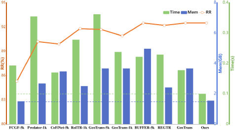
Figure 3: Comparison of running time and GPU memory consumption on 3DMatch dataset. At comparable registration recall, our method outperforms other methods in terms of running time and GPU memory.

4.1 Indoor Benchmarks: 3DMatch and 3DLoMatch

Dataset and Metrics.

The 3DMatch [65] dataset consists of $62$ indoor scenes, with $46$ scenes allocated for training, $8$ for validation, and $8$ for testing. The data is preprocessed and divided into two categories based on the level of overlap: 3DMatch (> $30\%$ overlap) and 3DLoMatch ($10\%$ $\sim$ $30\%$ overlap). In our experiments, we utilize this dataset to evaluate the real-world performance of our method as well as other methods. We assess the performance using Registration Recall (RR), denoting the fraction of point cloud pairs with transformation errors below a specified threshold (i.e., RMSE <$0.2m$). We also evaluate the Relative Translation Errors (RTE) and Relative Rotation Errors (RRE) to measure the accuracy of registrations. We introduce the implementation details in our supplementary material.

Methods	Estimator	Sample	3DMatch								3DLoMatch
			Time (s)↓				Mem	RR	RTE	RRE	Time (s)↓				Mem	RR	RTE	RRE
			Total	Data	Model	Pose	(GB)↓	(%)↑	(cm)↓	(°)↓	Total	Data	Model	Pose	(GB)↓	(%)↑	(cm)↓	(°)↓
REGTR [59]	RANSAC-$50k$	5000	1.283	0.016	0.217	1.050	2.413	86.7	5.3	1.774	1.031	0.015	0.211	0.785	2.264	50.5	8.2	3.005
RolTR [63]	RANSAC-$50k$	5000	0.384	0.022	0.214	0.148	2.507	91.1(91.9)	5.3	1.644	0.299	0.051	0.210	0.067	2.567	74.2(74.7)	7.8	2.554
GeoTrans [39]	RANSAC-$50k$	5000	0.362	0.091	0.079	0.192	3.669	91.7(92.0)	7.2	2.130	0.289	0.088	0.080	0.121	3.677	71.4(75.0)	12.6	3.558
Predator [30]	RANSAC-$50k$	1000	0.355	0.267	0.029	0.059	2.680	90.2(89.0)	6.6	2.015	0.351	0.267	0.028	0.056	2.241	57.8(56.7)	9.8	3.741
RolTR [63]	RANSAC-$50k$	1000	0.278	0.020	0.215	0.043	2.507	91.8(91.8)	5.6	1.690	0.259	0.052	0.209	0.008	2.567	74.1(74.8)	8.3	2.775
GeoTrans [39]	RANSAC-$50k$	1000	0.238	0.091	0.079	0.068	3.669	90.9(91.8)	7.5	2.225	0.198	0.088	0.080	0.030	3.677	69.8(74.2)	9.8	3.402
BUFFER [2]	RANSAC-$50k$	5000	0.222	0.033	0.186	0.003	4.976	92.5(92.9)	6.0	1.863	0.218	0.033	0.182	0.003	4.976	70.4(71.8)	10.1	3.018
FCGF [11]	RANSAC-$50k$	5000	0.193	0.006	0.036	0.151	1.500	85.3(85.1)	8.3	2.506	0.189	0.007	0.031	0.151	1.501	40.9(40.1)	10.1	3.134
CoFiNet [60]	RANSAC-$50k$	5000	0.170	0.030	0.091	0.049	3.472	89.9(89.3)	6.4	2.052	0.174	0.030	0.094	0.050	2.159	67.0(67.5)	9.0	3.180
REGTR [59]	weighted SVD	250	0.229	0.013	0.215	0.001	2.413	92.2(92.0)	4.9	1.562	0.221	0.014	0.206	0.001	2.328	64.5(64.8)	7.8	2.767
BUFFER [2]	weighted SVD	250	0.224	0.033	0.189	0.002	4.978	92.1	6.1	1.881	0.214	0.033	0.189	0.002	4.774	70.0	10.0	3.026
GeoTrans [39]	weighted SVD	250	0.172	0.091	0.079	0.002	3.669	86.7(86.5)	6.7	2.043	0.170	0.088	0.080	0.002	3.677	60.8(59.9)	10.2	3.709
Ours	weighted SVD	250	0.097	0.048	0.047	0.002	1.547	92.5	6.4	1.917	0.152	0.052	0.098	0.002	1.455	70.3	9.4	3.254
RolTR [63]	LGR	all	0.269	0.048	0.214	0.007	2.641	90.9	5.2	1.640	0.266	0.050	0.210	0.006	2.617	73.9	7.4	2.499
GeoTrans [39]	LGR	all	0.178	0.091	0.079	0.008	3.669	92.5(91.5)	6.3	1.808	0.175	0.088	0.080	0.007	3.677	74.0(74.0)	8.9	2.936
Ours	LGR	all	0.100	0.048	0.047	0.005	1.547	92.5	6.4	1.897	0.155	0.052	0.098	0.005	1.456	70.8	9.4	3.254

Table 1: Registration results on 3DMatch and 3DLoMatch. RR are the results obtained from our run and the results from the original paper (in parentheses). The best and second-best results are marked in underlined+bold and bold, and total runtime and GPU memory use green and blue to highlight for better displaying the efficiency advantages of our method.

Results.

Our method is compared with seven state-of-the-art (SOTA) models on registration results (RR), runtime (including data processing, model execution, pose estimation, and total time) and GPU memory usage on the 3DMatch and 3DLoMatch datasets, including FCGF [11], CoFiNet [60], Predator [30], GeoTrans [39], REGTR [59], RoITR [63] and BUFFER [2]. In order to ensure the fairness of the comparison, we test the comparison method multiple times in the same environment (using the official code and data), select the best results to display in the Tab. 1 and provide the RR of the original paper in parentheses. As shown in Tab. 1, for 3DMatch dataset, our method achieves the fastest running time and second slightest GPU memory usage. FCGF is the smallest GPU memory approach, but the registration recall is the worst among all methods and takes $93\%$ more time than our method. The runtime and the GPU memory usage comparison on 3DMatch are shown in Fig. 3. Compared with other methods, we improve the running time by at least $41\%$ and GPU memory by $38\%$ while achieving the best registration recall of $92.5$. On the 3DLoMatch dataset, although we fail to become the best method on RR, we are still the method with the fastest running speed and smallest GPU memory consumption. The visual results are shown in Fig. 4.

4.2 Outdoor Benchmark: KITTI odometry

Dataset and Metrics.

The KITTI odometry [21] dataset comprises $11$ LiDAR-scanned outdoor driving sequences. In line with previous work [4, 55], we partition the dataset into training sequences $0-5$, validation sequences $6-7$, and testing sequences $8-10$. Our method is assessed using three key metrics: Relative Rotation Error (RRE), Relative Translation Error (RTE), and Registration Recall (RR) which denotes the proportion of point cloud pairs meeting specific criteria (i.e., RRE <$5^{\circ}$ and RTE <$2m$).

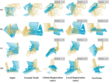
Figure 4: Registration results of our network for 3DLoMatch (a, b) and 3DMatch (c, d) with global and local registration. Compared to GeoTrans [39], our method has similar results in the global registration, and the local registration is further optimized to achieve superior results.

Results.

We compared our method with other methods FCGF [30], Predator [30], CoFiNet [60], GeoTrans [39] and BUFFER [2] on the KITTI dataset. Our approach achieves state-of-the-art (SOTA) performance on RR while surpassing the second fastest method by over $33\%$ in terms of runtime, and it attains the second smallest result in GPU memory consumption, using less than $2.4GB$. Although FCGF [11] consumes fewer GPU resources, it spends more time on pose estimation, leading to significantly longer runtime compared to other methods. Our network achieves comparable performance in RTE and RRE even though our sampling is sparser, and for the most critical registration metric RR, we achieve the best performance.

Method	Time	Mem	RTE	RRE	RR
	(s)↓	(GB)↓	(cm)↓	(°)↓	(%)↑
FCGF [11]	7.454	1.788	6.0	0.39	98.9
Predator [30]	0.703	4.634	6.8	0.26	99.8
CoFiNet [60]	0.201	3.055	8.2	0.41	99.8
GeoTrans [39]	0.251	3.666	6.2	0.23	99.8
BUFFER [2]	0.450	5.682	6.3	0.23	97.5
Our	0.168	2.304	7.8	0.34	99.8

Table 2: Registration results on KITTI odometry dataset. The best and second-best results are marked in bold and underline.

4.3 Ablation Study

Global and Local Encoder.

We test not using two identical encoders in global registration and local registration. For the global registration stage, the data of global sampling points pays more attention to learning the global representation. After multiple downsampling, the greater sparsity between global point clouds leads to larger feature differences between them. For the sampling points used in local registration, more emphasis is placed on learning local information within the neighborhood. Therefore, as shown in Tab. 3 (a), our method uses two encoders to facilitate enhanced feature learning at different stages, contributing to improved results.

Module	Model	3DMatch
		Time	RRE	RTE	RR
a. Encoder	1. single encoder	0.107	1.922	6.5	91.3
	2. Ours	0.100	1.897	6.4	92.5
b. Classifier	1. w/o classifier	0.279	1.983	6.6	91.3
	2. Ours	0.100	1.897	6.4	92.5
c. Mask	1. w/o mask	0.106	1.925	6.4	91.7
	2. gt mask	0.106	1.900	6.4	90.5
	3. Ours	0.100	1.897	6.4	92.5
d. Node	1. random nodes	0.094	1.871	6.3	90.9
	2. average center	0.089	1.884	6.4	90.7
	3. DBSCAN(Ours)	0.100	1.897	6.4	92.5
e. Iteration	1. iteration=0	0.081	1.884	6.4	90.7
	2. iteration=1	0.094	1.893	6.4	92.3
	3. iteration=2(Ours)	0.100	1.897	6.4	92.5
	4. iteration=3	0.105	1.900	6.4	92.5

Table 3: Ablation study on 3DMatch dataset.

Classifier.

We implement the early-exit mechanism for the iterative registration process by setting a numerical threshold for first-order spatial consistency ($SC$).

1. Without Classifier. We test the results without adding the classifier. As can be seen from Tab. 3 (b), the classifier achieves the purpose of reducing computing resources because it can effectively filter out a large number of simple registration scenarios.

2. Different Metrics. We assess the performance of model after the first local registration using different metrics as the classifier in Fig. 5, including inlier ratio (IR), second-order spatial consistency ($SC^{2}$) and $SC$. Based on the running time and registration recall of each metric, $SC$ performs the best.

3. Different Thresholds. We experimented with different global $SC$ thresholds $N_{g}$ and local $SC$ comparison threshold $N_{l}^{i}$ and the results are shown in Fig. 5. For the local registration stage, We initially set the threshold for the first local $SC$ comparison threshold $N_{l}^{1}$ to $0.1$ of the global $SC$ threshold and set the comparison threshold change difference to $\delta N_{l}^{i}$ ($\delta N_{l}^{i}$=$N_{l}^{1}$ by default), which represents the number of $N_{l}^{i+1}$ is reduced compared to $N_{l}^{i}$ each time (i.e., $N_{l}^{i}$=[$30$, $0$, $-30$…]).

Metrics	$N_{g}$	$\delta N_{l}^{i}$	RR	Time
$IR$	0.30	–	91.3	0.104
$SC^{2}$	300	–	91.6	0.107
$SC$	300	–	91.8	0.100
$SC$	$200$	20	92.0	0.094
	$300$	30	92.5	0.100
	$400$	40	92.2	0.109

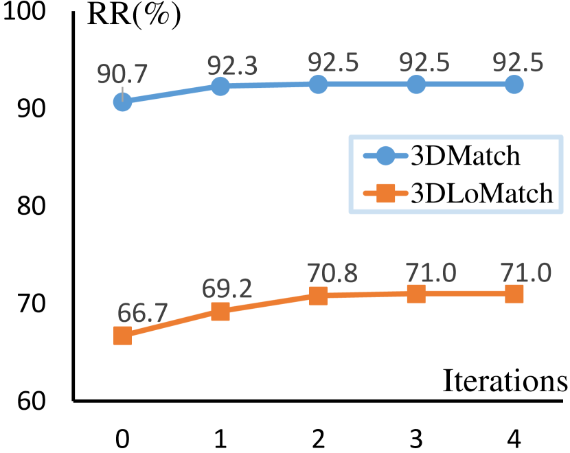
Figure 5: Left: Comparison of different metrics and different $SC$ thresholds ($N_{g}$). Right: The iteration results on 3DMatch/3DLoMatch demonstrates the effectiveness and stability of our iterations.

Overlap Mask.

We predict the overlap score in the training phase to calculate the overlap loss, which further supervises the point matching. Introducing the overlap mask to filter the paired points eliminates the interference of outliers for the patch proposal in the next registration process. As can be seen from Tab. 3 (c), by using the ground truth label as the mask and not using the mask for comparison, the experiment proves that our method uses the overlap score as the mask to obtain the best result.

Refined Node Proposal Module.

Before performing local registration, we utilize the refined nodes proposal module to select new nodes for registration based on the global matched points obtained from the last registration. We compare the DBSCAN clustering algorithm with random sampling and global centers methods, and the results in Tab. 3 (d) demonstrate that while our method may consume more time, it significantly improves the registration results.

Iteration.

In order to prove the effect of iteration of our method, we compare the method global registration Tab. 3 (e.1) without iteration with the method using local registration multiple times Tab. 3 (e.2-4) for iteration. Additionally, we plot the iterative results in the line chart shown in Fig. 5 on the 3DMatch and 3DLomatch datasets. As the number of iterations increases, the registration result reaches the optimum in the second iteration, and the result remains unchanged in subsequent iterations. However, during multiple iterations, the RRE continues to increase. This is because, in the process of dynamically finding the registration region, our model continues to reduce the number and region of registration points, which will affect the finer-grained accuracy in some scenes. But it still performs well on the more important metric RR.

5 Conclusion

In this paper, we innovatively introduce dynamic networks into the task of point cloud registration and propose a fast and efficient dynamic point cloud registration network. We use sparser global sampling to process the input point cloud to reduce significantly the computational complexity of the network, and use an iterative approach to perform multiple registrations and continuously narrow down the registration region to eliminate interference from outliers. This process terminates once the registration result meets the classifier condition threshold, leading to an adaptive inference paradigm. The Refined Nodes Proposal module is employed to discover the inliers concentration region among the paired points obtained in the previous registration for the next registration, which further improves the accuracy of the registration without increasing excessive computational consumption. Extensive experiments demonstrate that our method achieves the fastest runtime on both indoor and outdoor datasets while maintaining competitive results.

Supplementary Material

Appendix A Implementation Details

Our proposed method was implemented by PyTorch. To ensure fairness, we employed the official code and pre-trained models provided by the baseline methods for comparison. All experiments were performed on the same PC with an Intel Core i7-12700K CPU and a single Nvidia RTX 3090 with $24G$ memory. We train the model for $40$ epochs on both 3DMatch [65] and KITTI [21] with the batch size was set to $1$. We use an Adam optimizer with an initial learning rate of $1e-4$, which is exponentially decayed by $0.05$ every epoch for 3DMatch and every $4$ epoch for KITTI. We set the numbers of downsampling layers as $5$ for the 3DMatch dataset and $6$ for the KITTI dataset. The numbers of points in the patch are set to $32$ and $64$, respectively. Other parameters remain consistent with GeoTrans [39]. Network architectures are detailed as follows:

KPconv Network.

We use the KPConv [48] network as our backbone for multi-level downsampling and feature extraction. The specific structure is the same as GeoTrans [39]. First, the input point cloud is sampled using grid downsampling with a voxel size of $2.5cm$ on 3DMatch/3DLoMatch and $30cm$ on KITTI. With each subsequent downsampling operation, the voxel size is doubled. We use deeper sampling to obtain sparser point clouds, respectively, 4-stage for 3DMatch and 5-stage for KITTI. The numbers of calibrated neighbors used for downsampling are [37, 36, 36, 38, 36] for 3DMatch and [65, 63, 70, 74, 69, 58] for KITTI. Other settings are consistent with GeoTrans [39].

Geometric Transformer Encoder.

We use the Geometric Transformer in GeoTrans [39] as our encoder in the global registration stage and local registration stage. Firstly, the encoder receives the features from KPConv and projects them to $d=256$ for 3DMatch/3DLoMatch and $d=128$ dimensions for KITTI. For the Local encoder, since the features come from the third level of KPConv sampling, the dimensions are from $512$ to $256$ and $512$ to $128$ when performing feature projection. Then after three alternations of ’self-attention and cross-attention’, the features are obtained and used for pairing point sets through feed-forward networks (FFN).

Classifier.

In the inference phase, for the classifier threshold, we set the global $SC$ threshold to $300$ for the 3DMatch dataset, and the local $SC$ comparison threshold (limiting the reduction in the number of pairs) to [$30$, $0$, $-30$, …]. Similarly, for 3DLoMatch, we set the global threshold to $200$ and the iteration threshold to [$40$, $0$, $-40$, …], and for KITTI, we set the global threshold to $30$ and the iteration threshold to [$10$, $0$, …].

Appendix B Loss Function

Coarse Matching Loss.

We use the overlap-aware circle loss to supervise the point-wise feature descriptors and focus the model on matches with high overlap following GeoTrans [39]. The overall coarse matching loss is $\mathcal{L}_{c}=(\mathcal{L}_{c}^{Q}+\mathcal{L}_{c}^{P})/2$. Consider a pair of overlapping point clouds $P$ and $Q$ aligned by ground truth transformation. We choose the points $p_{i}\in P$ that have at least one correspondence in $Q$ to form a set of anchor patches, denoted as $\mathcal{A}$. For each anchor patch $\mathcal{G}_{i}^{\mathcal{P}}\in\mathcal{A}$, we consider the paired patches are positive if they share a minimum overlap of $10\%$, and negative if they have no overlap. We identify the set of its positive patches in $Q$ as $\varepsilon_{p}^{i}$, and the set of its negative patches as $\varepsilon_{n}^{i}$. The coarse matching loss on $P$ is defined as:

$$\small\mathcal{L}_{c}^{P}\!=\!\frac{1}{|\mathcal{A}|}\!\sum_{\mathcal{G}_{i}^{\mathcal{P}}\in\mathcal{A}}log[1+\!\!\sum_{\mathcal{G}_{j}^{\mathcal{Q}}\in\varepsilon_{p}^{i}}\!e^{\lambda_{i}^{j}\beta_{p}^{i,j}(d_{i}-\Delta_{p})}\!\cdot\!\!\sum_{\mathcal{G}_{k}^{\mathcal{Q}}\in\varepsilon_{n}^{i}}\!\!e^{\beta_{n}^{i,k}(\Delta_{n}-d_{i}^{k})}]$$ (11)

where $d_{i}^{j}=||f_{p_{i}}-f_{q_{j}}||_{2}$ is the feature distance, $\lambda_{i}^{j}=(o_{i}^{j})^{\frac{1}{2}}$ and $o_{i}^{j}$ represents the overlap ratio between $\mathcal{G}_{i}^{\mathcal{P}}$ and $\mathcal{G}_{j}^{\mathcal{Q}}$. $\beta_{p}^{i,j}$ and $\beta_{n}^{i,k}$ are the positive and negative weights respectively, $\Delta_{n}$ and $\Delta_{p}$ are the margin hyper-parameters which are set to $0.1$ and $1.4$. The same goes for the loss $\mathcal{L}_{c}^{Q}$ on $Q$.

Point Matching Loss.

During training, we randomly sample $N_{g}$ ground-truth node correspondences $\hat{C_{i}^{*}}$ instead of using the predicted ones. We employ a negative log-likelihood loss [44] on the assignment matrix $\bar{C}_{i}$ for each sparse correspondences. The point matching loss is calculated by taking the average of the individual losses across all points correspondences: $\mathcal{L}_{p}=\frac{1}{N_{g}}{\textstyle\sum_{i=1}^{N_{g}}}\mathcal{L}_{p,i}$. For each correspondence, a set of paired point $\mathcal{M}_{i}$ is extracted with a matching radius $\tau$. The unmatched points in the two patches are represented by $\mathcal{I}_{i}$ and $\mathcal{J}_{i}$. The individual point matching loss for correspondence $\hat{C_{i}^{*}}$ is computed as:

$$\mathcal{L}_{p,i}\!=\!-\!\!\sum_{(x,y)\in\mathcal{M}_{i}}\!\!log\bar{C}_{x,y}^{i}\!-\!\sum_{x\in\mathcal{I}_{i}}\!log\bar{C}_{x,m_{i}+1}^{i}\!-\!\sum_{y\in\mathcal{J}_{i}}\!log\bar{C}_{n_{i}+1,y}^{i}$$ (12)

Appendix C Metrics

We use the same metrics for 3DMatch/3DLoMatch and KITTI datasets, namely RTE, RRE, RR respectively.

Relative Translation Error (RTE).

RTE specifically focuses on the translation component of the registration error. It measures the Euclidean distance between the true translation and the estimated translation achieved during the registration process. RTE provides insight into how well the registration algorithm performs in terms of aligning the point clouds along the translation axes.

$$RTE=||t_{est}-t_{gt}||$$ (13)

where $t_{est}$ and $t_{gt}$ denote the estimated translation vector and ground truth translation vector, respectively. $||\cdot||$ represents the Euclidean norm

Relative Rotation Error (RRE).

RRE measures the angular difference between the true rotation and the estimated rotation after point cloud registration. It is a measure of how well the rotational alignment has been achieved.

$$RRE=\arccos(\frac{trace(R^{T}_{est}R_{gt})-1}{2})$$ (14)

where $R_{est}$ and $R_{gt}$ denote the estimated rotation matrix and ground truth rotation matrix, respectively. $arccos(\cdot)$ is the inverse cosine function, $trace(~{}\cdot)$ represents the trace of the matrix.

Registration Recall (RR).

Registration Recall is a measure of the accuracy of point cloud registration, specifically focusing on the overall transformation quality, considering both rotation and translation.

For 3DMatch/3DLoMatch, RR is computed based on the Root Mean Square Error (RMSE), which is used to measure the distance error between two point clouds. For the set of ground truth correspondences $C$ after applying the estimated transformation $T_{est}$, the calculation formula of RMSE is as follows:

$$RMSE=\sqrt{\frac{1}{|C|}{\sum_{(p_{i},q_{i})\in C}||T_{est}(p_{i})-q_{i}||^{2}}}$$ (15)

where $|C|$ is the number of correspondence set, $p_{i}$, $q_{i}$ are the i-th pair of paired points in the set of ground truth correspondences $C$. Lower RMSE values correspond to better alignment accuracy. RR is defined as:

$$RR=\frac{1}{|C|}\sum_{i=1}^{C}[RMSE_{i}<\tau_{RMSE}]$$ (16)

where $\tau_{RMSE}$ is $0.2m$.

Module	Model	3DLoMatch
		Time	RRE	RTE	RR
a. Encoder	1. single encoder	0.275	3.251	9.5	66.9
	2. Ours	0.155	3.233	9.4	70.8
b. Classifier	1. w/o classifier	0.279	1.983	8.6	62.6
	2. Ours	0.155	3.233	9.4	70.8
c. Mask	1. w/o mask	0.150	3.259	9.5	66.0
	2. gt mask	0.149	3.231	9.3	65.8
	3. Ours	0.155	3.233	9.4	70.8
d. Node	1. random nodes	0.098	3.176	9.1	63.5
	2. average center	0.079	3.223	9.2	63.0
	3. DBSCAN(Ours)	0.155	3.233	9.4	70.8
e. Iteration	1. iteration=0	0.080	3.179	9.2	66.7
	2. iteration=1	0.121	3.203	9.2	69.2
	3. iteration=2(Ours)	0.155	3.233	9.4	70.8
	4. iteration=3	0.175	3.199	9.3	71.0
	5. iteration=4	0.176	3.199	9.3	71.0

Table 4: Ablation study on 3DLoMatch dataset. Our experiments keep the same settings as the 3DMatch dataset.

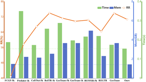
Figure 6: Comparison of running time and GPU memory consumption on 3DLoMatch dataset. Our method outperforms other methods in terms of running time and GPU memory while possessing competitive registration recall (RR).

For KITTI, RR is defined as the ratio of point cloud pairs for which both the Relative Rotation Error (RRE) and Relative Translation Error (RTE) are below specific thresholds (i.e., RRE $<5^{\circ}$ and RTE $<2m$):

$$RR=\frac{1}{|C|}\sum_{i}^{C}[RRE_{i}<5^{\circ}\wedge RTE_{i}<2m]$$ (17)

Appendix D Additional Experiments

Ablation Study on 3DLoMatch.

We perform an ablation study on the 3DLoMatch dataset, as shown in the Tab. 4. Similar to the experiment on the 3DMatch dataset in the main paper, we verify each block of our model separately and adopt the same experimental settings. The results prove that our default settings achieve the best performance.

Comparison of results on the 3DLoMatch.

As can be seen from Fig. 6, our method still has advantages in running time and GPU memory usage. Compared with the second fastest running method (such as Predator [30]), as well as other lightweight methods (such as FCGF [11], REGTR [59]), they all have a greater impact on the registration results on the 3DLoMatch dataset, and our method can still maintain Registration Recall of 70.8%.

Appendix E Additional Qualitative Results

We provide the registration results on KITTI in the Fig. 7. Our method achieves higher accuracy on the KITTI dataset.

We also provide more visualized results of our method on 3DMatch/3DLoMatch in Fig. 8, and the registration results of GeoTrans [39] are shown for comparison.

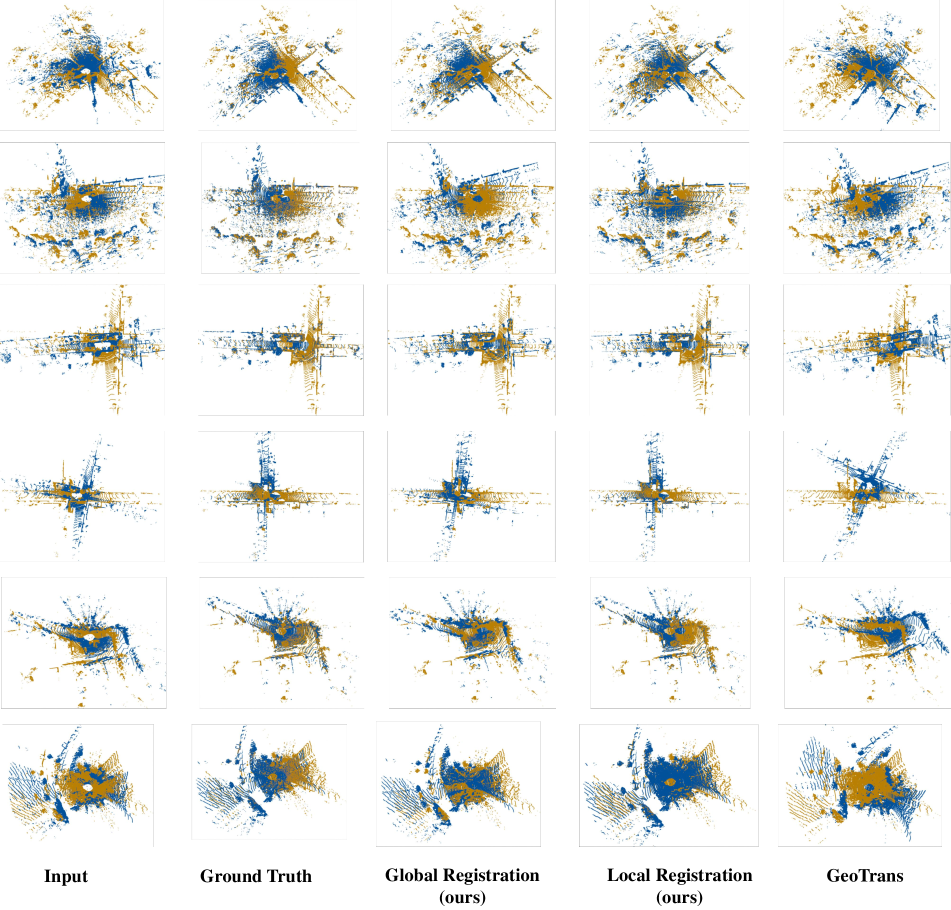
Figure 7: Registration results on KITTI. Our method achieves higher accuracy after local registration and achieves good performance similar to ground truth.

The performance of our method in global registration is similar to that of GeoTrans. For example, in the 5th and 6th scenes of Fig. 8, global registration has a large error with the ground truth. However, after local registration, our method achieves significant improvements and finally obtains the correct registration result.

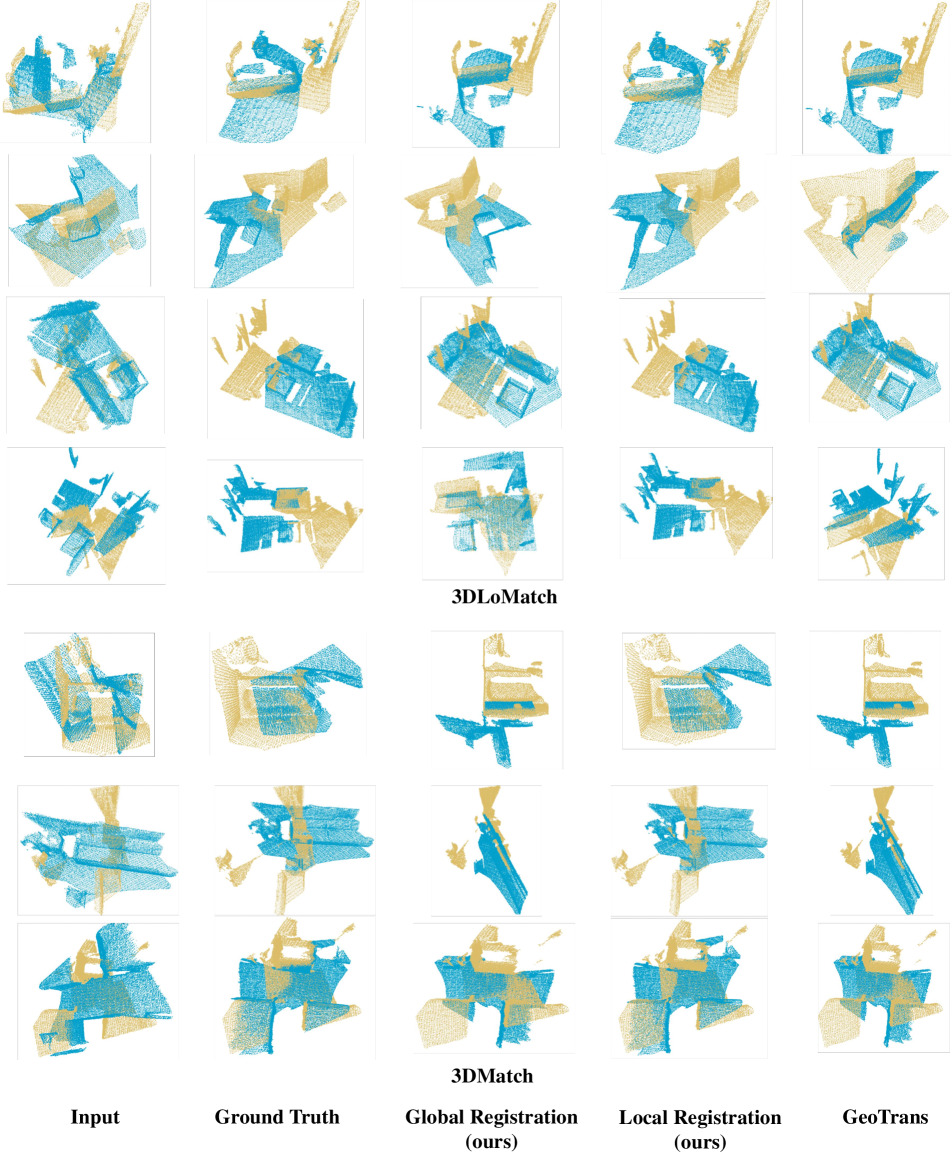
Figure 8: Registration results on 3DMatch and 3DLoMatch. The global registration in our method has similar results to the comparative method GeoTrans [39], while the further optimization of our local registration achieves more accurate results.

References

- Ao et al. [2021] Sheng Ao, Qingyong Hu, Bo Yang, Andrew Markham, and Yulan Guo. Spinnet: Learning a general surface descriptor for 3d point cloud registration. In Proceedings of the IEEE/CVF conference on computer vision and pattern recognition, pages 11753–11762, 2021.
- Ao et al. [2023] Sheng Ao, Qingyong Hu, Hanyun Wang, Kai Xu, and Yulan Guo. Buffer: Balancing accuracy, efficiency, and generalizability in point cloud registration. In Proceedings of the IEEE/CVF Conference on Computer Vision and Pattern Recognition, pages 1255–1264, 2023.
- Aoki et al. [2019] Yasuhiro Aoki, Hunter Goforth, Rangaprasad Arun Srivatsan, and Simon Lucey. Pointnetlk: Robust & efficient point cloud registration using pointnet. In Proceedings of the IEEE/CVF conference on computer vision and pattern recognition, pages 7163–7172, 2019.
- Bai et al. [2021] Xuyang Bai, Zixin Luo, Lei Zhou, Hongkai Chen, Lei Li, Zeyu Hu, Hongbo Fu, and Chiew-Lan Tai. Pointdsc: Robust point cloud registration using deep spatial consistency. In Proceedings of the IEEE/CVF Conference on Computer Vision and Pattern Recognition, pages 15859–15869, 2021.
- Barath and Matas [2018] Daniel Barath and Jiří Matas. Graph-cut ransac. In Proceedings of the IEEE conference on computer vision and pattern recognition, pages 6733–6741, 2018.
- Cao et al. [2019] Shijie Cao, Lingxiao Ma, Wencong Xiao, Chen Zhang, Yunxin Liu, Lintao Zhang, Lanshun Nie, and Zhi Yang. Seernet: Predicting convolutional neural network feature-map sparsity through low-bit quantization. In Proceedings of the IEEE/CVF Conference on Computer Vision and Pattern Recognition, pages 11216–11225, 2019.
- Chen et al. [2021] Jin Chen, Xijun Wang, Zichao Guo, Xiangyu Zhang, and Jian Sun. Dynamic region-aware convolution. In Proceedings of the IEEE/CVF conference on computer vision and pattern recognition, pages 8064–8073, 2021.
- Chen et al. [2022a] Zhilei Chen, Honghua Chen, Lina Gong, Xuefeng Yan, Jun Wang, Yanwen Guo, Jing Qin, and Mingqiang Wei. Utopic: Uncertainty-aware overlap prediction network for partial point cloud registration. In Computer Graphics Forum, pages 87–98. Wiley Online Library, 2022a.
- Chen et al. [2022b] Zhi Chen, Kun Sun, Fan Yang, and Wenbing Tao. Sc2-pcr: A second order spatial compatibility for efficient and robust point cloud registration. In Proceedings of the IEEE/CVF Conference on Computer Vision and Pattern Recognition, pages 13221–13231, 2022b.
- Chen et al. [2023] Zhi Chen, Kun Sun, Fan Yang, Lin Guo, and Wenbing Tao. Sc2-pcr++: Rethinking the generation and selection for efficient and robust point cloud registration. IEEE Transactions on Pattern Analysis and Machine Intelligence, 2023.
- Choy et al. [2019] Christopher Choy, Jaesik Park, and Vladlen Koltun. Fully convolutional geometric features. In Proceedings of the IEEE/CVF international conference on computer vision, pages 8958–8966, 2019.
- Choy et al. [2020] Christopher Choy, Wei Dong, and Vladlen Koltun. Deep global registration. In Proceedings of the IEEE/CVF conference on computer vision and pattern recognition, pages 2514–2523, 2020.
- Chu and Nie [2011] Jun Chu and Chun-mei Nie. Multi-view point clouds registration and stitching based on sift feature. In 2011 3rd International Conference on Computer Research and Development, pages 274–278. IEEE, 2011.
- Deng et al. [2018] Haowen Deng, Tolga Birdal, and Slobodan Ilic. Ppfnet: Global context aware local features for robust 3d point matching. In Proceedings of the IEEE conference on computer vision and pattern recognition, pages 195–205, 2018.
- Deng et al. [2019] Haowen Deng, Tolga Birdal, and Slobodan Ilic. 3d local features for direct pairwise registration. In Proceedings of the IEEE/CVF conference on computer vision and pattern recognition, pages 3244–3253, 2019.
- Dong et al. [2017] Xuanyi Dong, Junshi Huang, Yi Yang, and Shuicheng Yan. More is less: A more complicated network with less inference complexity. In Proceedings of the IEEE conference on computer vision and pattern recognition, pages 5840–5848, 2017.
- Ester et al. [1996] Martin Ester, Hans-Peter Kriegel, Jörg Sander, Xiaowei Xu, et al. A density-based algorithm for discovering clusters in large spatial databases with noise. In kdd, pages 226–231, 1996.
- Fan et al. [2018] Hehe Fan, Zhongwen Xu, Linchao Zhu, Chenggang Yan, Jianjun Ge, and Yi Yang. Watching a small portion could be as good as watching all: Towards efficient video classification. In IJCAI International Joint Conference on Artificial Intelligence, 2018.
- Fischler and Bolles [1981] Martin A Fischler and Robert C Bolles. Random sample consensus: a paradigm for model fitting with applications to image analysis and automated cartography. Communications of the ACM, 24(6):381–395, 1981.
- Fragoso et al. [2013] Victor Fragoso, Pradeep Sen, Sergio Rodriguez, and Matthew Turk. Evsac: accelerating hypotheses generation by modeling matching scores with extreme value theory. In Proceedings of the IEEE international conference on computer vision, pages 2472–2479, 2013.
- Geiger et al. [2012] Andreas Geiger, Philip Lenz, and Raquel Urtasun. Are we ready for autonomous driving? the kitti vision benchmark suite. In 2012 IEEE conference on computer vision and pattern recognition, pages 3354–3361. IEEE, 2012.
- Ghodrati et al. [2021] Amir Ghodrati, Babak Ehteshami Bejnordi, and Amirhossein Habibian. Frameexit: Conditional early exiting for efficient video recognition. In Proceedings of the IEEE/CVF Conference on Computer Vision and Pattern Recognition, pages 15608–15618, 2021.
- Han et al. [2021] Yizeng Han, Gao Huang, Shiji Song, Le Yang, Honghui Wang, and Yulin Wang. Dynamic neural networks: A survey. IEEE Transactions on Pattern Analysis and Machine Intelligence, 44(11):7436–7456, 2021.
- Han et al. [2022] Yizeng Han, Yifan Pu, Zihang Lai, Chaofei Wang, Shiji Song, Junfeng Cao, Wenhui Huang, Chao Deng, and Gao Huang. Learning to weight samples for dynamic early-exiting networks. In European Conference on Computer Vision, pages 362–378. Springer, 2022.
- Herrmann et al. [2020] Charles Herrmann, Richard Strong Bowen, and Ramin Zabih. Channel selection using gumbel softmax. In European Conference on Computer Vision, pages 241–257. Springer, 2020.
- Hosseini and Timmerer [2018] Mohammad Hosseini and Christian Timmerer. Dynamic adaptive point cloud streaming. In Proceedings of the 23rd Packet Video Workshop, pages 25–30, 2018.
- Howard et al. [2017] Andrew G Howard, Menglong Zhu, Bo Chen, Dmitry Kalenichenko, Weijun Wang, Tobias Weyand, Marco Andreetto, and Hartwig Adam. Mobilenets: Efficient convolutional neural networks for mobile vision applications. arXiv preprint arXiv:1704.04861, 2017.
- Hu et al. [2019] Xuecai Hu, Haoyuan Mu, Xiangyu Zhang, Zilei Wang, Tieniu Tan, and Jian Sun. Meta-sr: A magnification-arbitrary network for super-resolution. In Proceedings of the IEEE/CVF conference on computer vision and pattern recognition, pages 1575–1584, 2019.
- Huang and Chen [2018] Gao Huang and Danlu Chen. Multi-scale dense networks for resource efficient image classification. ICLR 2018, 2018.
- [30] Shengyu Huang, Zan Gojcic, and Mikhail Usvyatsov Andreas Wieser Konrad Schindler. Predator: Registration of 3d point clouds with low overlap-supplementary material.
- Jiang et al. [2021] Haobo Jiang, Jin Xie, Jianjun Qian, and Jian Yang. Planning with learned dynamic model for unsupervised point cloud registration. arXiv preprint arXiv:2108.02613, 2021.
- Kostavelis and Gasteratos [2015] Ioannis Kostavelis and Antonios Gasteratos. Semantic mapping for mobile robotics tasks: A survey. Robotics and Autonomous Systems, 66:86–103, 2015.
- Lazebnik et al. [2005] Svetlana Lazebnik, Cordelia Schmid, and Jean Ponce. A sparse texture representation using local affine regions. IEEE transactions on pattern analysis and machine intelligence, 27(8):1265–1278, 2005.
- Li et al. [2019] Hao Li, Hong Zhang, Xiaojuan Qi, Ruigang Yang, and Gao Huang. Improved techniques for training adaptive deep networks. In Proceedings of the IEEE/CVF international conference on computer vision, pages 1891–1900, 2019.
- Meng et al. [2022] Lingchen Meng, Hengduo Li, Bor-Chun Chen, Shiyi Lan, Zuxuan Wu, Yu-Gang Jiang, and Ser-Nam Lim. Adavit: Adaptive vision transformers for efficient image recognition. In Proceedings of the IEEE/CVF Conference on Computer Vision and Pattern Recognition, pages 12309–12318, 2022.
- Meng et al. [2020] Yue Meng, Rameswar Panda, Chung-Ching Lin, Prasanna Sattigeri, Leonid Karlinsky, Kate Saenko, Aude Oliva, and Rogerio Feris. Adafuse: Adaptive temporal fusion network for efficient action recognition. In International Conference on Learning Representations, 2020.
- Pais et al. [2020] G Dias Pais, Srikumar Ramalingam, Venu Madhav Govindu, Jacinto C Nascimento, Rama Chellappa, and Pedro Miraldo. 3dregnet: A deep neural network for 3d point registration. In Proceedings of the IEEE/CVF conference on computer vision and pattern recognition, pages 7193–7203, 2020.
- Qi et al. [2017] Charles R Qi, Hao Su, Kaichun Mo, and Leonidas J Guibas. Pointnet: Deep learning on point sets for 3d classification and segmentation. In Proceedings of the IEEE conference on computer vision and pattern recognition, pages 652–660, 2017.
- Qin et al. [2022] Zheng Qin, Hao Yu, Changjian Wang, Yulan Guo, Yuxing Peng, and Kai Xu. Geometric transformer for fast and robust point cloud registration. In Proceedings of the IEEE/CVF conference on computer vision and pattern recognition, pages 11143–11152, 2022.
- Ren et al. [2018] Mengye Ren, Andrei Pokrovsky, Bin Yang, and Raquel Urtasun. Sbnet: Sparse blocks network for fast inference. In Proceedings of the IEEE Conference on Computer Vision and Pattern Recognition, pages 8711–8720, 2018.
- Rusu et al. [2009] Radu Bogdan Rusu, Andreas Holzbach, Nico Blodow, and Michael Beetz. Fast geometric point labeling using conditional random fields. In 2009 IEEE/RSJ International Conference on Intelligent Robots and Systems, pages 7–12. IEEE, 2009.
- Salti et al. [2014] Samuele Salti, Federico Tombari, and Luigi Di Stefano. Shot: Unique signatures of histograms for surface and texture description. Computer Vision and Image Understanding, 125:251–264, 2014.
- Sandler et al. [2018] Mark Sandler, Andrew Howard, Menglong Zhu, Andrey Zhmoginov, and Liang-Chieh Chen. Mobilenetv2: Inverted residuals and linear bottlenecks. In Proceedings of the IEEE conference on computer vision and pattern recognition, pages 4510–4520, 2018.
- Sarlin et al. [2020] Paul-Edouard Sarlin, Daniel DeTone, Tomasz Malisiewicz, and Andrew Rabinovich. Superglue: Learning feature matching with graph neural networks. In Proceedings of the IEEE/CVF conference on computer vision and pattern recognition, pages 4938–4947, 2020.
- Sarode et al. [2019] Vinit Sarode, Xueqian Li, Hunter Goforth, Yasuhiro Aoki, Rangaprasad Arun Srivatsan, Simon Lucey, and Howie Choset. Pcrnet: Point cloud registration network using pointnet encoding. arXiv preprint arXiv:1908.07906, 2019.
- Sun et al. [2021] Ximeng Sun, Rameswar Panda, Chun-Fu Richard Chen, Aude Oliva, Rogerio Feris, and Kate Saenko. Dynamic network quantization for efficient video inference. In Proceedings of the IEEE/CVF International Conference on Computer Vision, pages 7375–7385, 2021.
- Tang et al. [2021] Jiapeng Tang, Dan Xu, Kui Jia, and Lei Zhang. Learning parallel dense correspondence from spatio-temporal descriptors for efficient and robust 4d reconstruction. In Proceedings of the IEEE/CVF Conference on Computer Vision and Pattern Recognition, pages 6022–6031, 2021.
- Thomas et al. [2019] Hugues Thomas, Charles R Qi, Jean-Emmanuel Deschaud, Beatriz Marcotegui, François Goulette, and Leonidas J Guibas. Kpconv: Flexible and deformable convolution for point clouds. In Proceedings of the IEEE/CVF international conference on computer vision, pages 6411–6420, 2019.
- Veit and Belongie [2018] Andreas Veit and Serge Belongie. Convolutional networks with adaptive inference graphs. In Proceedings of the European Conference on Computer Vision (ECCV), pages 3–18, 2018.
- Verelst and Tuytelaars [2020] Thomas Verelst and Tinne Tuytelaars. Dynamic convolutions: Exploiting spatial sparsity for faster inference. In Proceedings of the ieee/cvf conference on computer vision and pattern recognition, pages 2320–2329, 2020.
- Wang et al. [2022a] Haiping Wang, Yuan Liu, Zhen Dong, and Wenping Wang. You only hypothesize once: Point cloud registration with rotation-equivariant descriptors. In Proceedings of the 30th ACM International Conference on Multimedia, pages 1630–1641, 2022a.
- Wang et al. [2020] Yulin Wang, Kangchen Lv, Rui Huang, Shiji Song, Le Yang, and Gao Huang. Glance and focus: a dynamic approach to reducing spatial redundancy in image classification. Advances in Neural Information Processing Systems, 33:2432–2444, 2020.
- Wang et al. [2022b] Yulin Wang, Yang Yue, Yuanze Lin, Haojun Jiang, Zihang Lai, Victor Kulikov, Nikita Orlov, Humphrey Shi, and Gao Huang. Adafocus v2: End-to-end training of spatial dynamic networks for video recognition. In 2022 IEEE/CVF Conference on Computer Vision and Pattern Recognition (CVPR), pages 20030–20040. IEEE, 2022b.
- Yang et al. [2019] Brandon Yang, Gabriel Bender, Quoc V Le, and Jiquan Ngiam. Condconv: Conditionally parameterized convolutions for efficient inference. Advances in neural information processing systems, 32, 2019.
- Yang et al. [2022] Fan Yang, Lin Guo, Zhi Chen, and Wenbing Tao. One-inlier is first: Towards efficient position encoding for point cloud registration. Advances in Neural Information Processing Systems, 35:6982–6995, 2022.
- Yang et al. [2020] Heng Yang, Jingnan Shi, and Luca Carlone. Teaser: Fast and certifiable point cloud registration. IEEE Transactions on Robotics, 37(2):314–333, 2020.
- Yeung et al. [2016] Serena Yeung, Olga Russakovsky, Greg Mori, and Li Fei-Fei. End-to-end learning of action detection from frame glimpses in videos. In Proceedings of the IEEE conference on computer vision and pattern recognition, pages 2678–2687, 2016.
- Yew and Lee [2020] Zi Jian Yew and Gim Hee Lee. Rpm-net: Robust point matching using learned features. In Proceedings of the IEEE/CVF conference on computer vision and pattern recognition, pages 11824–11833, 2020.
- Yew and Lee [2022] Zi Jian Yew and Gim Hee Lee. Regtr: End-to-end point cloud correspondences with transformers. In Proceedings of the IEEE/CVF conference on computer vision and pattern recognition, pages 6677–6686, 2022.
- Yu et al. [2021] Hao Yu, Fu Li, Mahdi Saleh, Benjamin Busam, and Slobodan Ilic. Cofinet: Reliable coarse-to-fine correspondences for robust pointcloud registration. Advances in Neural Information Processing Systems, 34:23872–23884, 2021.
- Yu et al. [2022] Hao Yu, Ji Hou, Zheng Qin, Mahdi Saleh, Ivan Shugurov, Kai Wang, Benjamin Busam, and Slobodan Ilic. Riga: Rotation-invariant and globally-aware descriptors for point cloud registration. arXiv preprint arXiv:2209.13252, 2022.
- Yu et al. [2023a] Haichao Yu, Haoxiang Li, Gang Hua, Gao Huang, and Humphrey Shi. Boosted dynamic neural networks. In Proceedings of the AAAI Conference on Artificial Intelligence, pages 10989–10997, 2023a.
- Yu et al. [2023b] Hao Yu, Zheng Qin, Ji Hou, Mahdi Saleh, Dongsheng Li, Benjamin Busam, and Slobodan Ilic. Rotation-invariant transformer for point cloud matching. In Proceedings of the IEEE/CVF Conference on Computer Vision and Pattern Recognition, pages 5384–5393, 2023b.
- Yurtsever et al. [2020] Ekim Yurtsever, Jacob Lambert, Alexander Carballo, and Kazuya Takeda. A survey of autonomous driving: Common practices and emerging technologies. IEEE access, 8:58443–58469, 2020.
- Zeng et al. [2017] Andy Zeng, Shuran Song, Matthias Nießner, Matthew Fisher, Jianxiong Xiao, and Thomas Funkhouser. 3dmatch: Learning local geometric descriptors from rgb-d reconstructions. In Proceedings of the IEEE conference on computer vision and pattern recognition, pages 1802–1811, 2017.
- Zhang et al. [2023] Xiyu Zhang, Jiaqi Yang, Shikun Zhang, and Yanning Zhang. 3d registration with maximal cliques. In Proceedings of the IEEE/CVF Conference on Computer Vision and Pattern Recognition, pages 17745–17754, 2023.
- Zhang et al. [2022] Yu Zhang, Junle Yu, Xiaolin Huang, Wenhui Zhou, and Ji Hou. Pcr-cg: Point cloud registration via deep explicit color and geometry. In European Conference on Computer Vision, pages 443–459. Springer, 2022.
- Zhou et al. [2016] Bolei Zhou, Aditya Khosla, Agata Lapedriza, Aude Oliva, and Antonio Torralba. Learning deep features for discriminative localization. In Proceedings of the IEEE conference on computer vision and pattern recognition, pages 2921–2929, 2016.