Semi-Supervised Health Index Monitoring with Feature Generation and Fusion

Abstract

The Health Index (HI) is crucial for evaluating system health, aiding tasks like anomaly detection and predicting remaining useful life for systems demanding high safety and reliability. Tight monitoring is crucial for achieving high precision at a lower cost, with applications such as spray coating. Obtaining HI labels in real-world applications is often cost-prohibitive, requiring continuous, precise health measurements. Therefore, it is more convenient to leverage run-to failure datasets that may provide potential indications of machine wear condition, making it necessary to apply semi-supervised tools for HI construction. In this study, we adapt the Deep Semi-supervised Anomaly Detection (DeepSAD) method for HI construction. We use the DeepSAD embedding as a condition indicators to address interpretability challenges and sensitivity to system-specific factors. Then, we introduce a diversity loss to enrich condition indicators. We employ an alternating projection algorithm with isotonic constraints to transform the DeepSAD embedding into a normalized HI with an increasing trend. Validation on the PHME 2010 milling dataset, a recognized benchmark with ground truth HIs demonstrates meaningful HIs estimations. Our methodology is then applied to monitor wear states of thermal spray coatings using high-frequency voltage. Our contributions create opportunities for more accessible and reliable HI estimation, particularly in cases where obtaining ground truth HI labels is unfeasible.

I Introduction

Thermal spray coating, is a materials processing technique used to apply protective or decorative coatings to various surfaces. Major customers for thermal spray products include jet engine, gas turbine, and automobile manufacturers. Nevertheless, customers in the thermal spray coating industry allocate substantial funds annually to verify coating quality and and fixing parts with low coating quality. The Health Index (HI), alternatively referred to as a health indicator, serves as an indicator reflecting the operational state and overall health condition of a system [1]. It frequently serves as a important metric for subsequent prognostics and health manamgement (PHM) tasks, such as anomaly detection [2], condition monitoring [3], and prediction of remaining useful life [4]. At present, there is a shortage of appropriate tools available in the market for monitoring the HI of thermal spray coatings. In this work, we propose a model that derive an HI from the high-frequency voltage signal from the spray coating system. Utilizing the high-frequency voltage signal as an input offers the benefit of enabling non-intrusive quality monitoring without the need for adjustments to the spraying system.

The data-driven strategies for estimating the Health Index (HI) can be categorized into three main groups: supervised, unsupervised, or semi-supervised. Supervised HI estimation requires either a direct or indirect measurement of the ground truth health index. For instance, in the case of the PHME 2010 Milling dataset [5], which includes run-to-failure data from a cutting tool, a measurement of the degradation of each flank wear on the three cutting edges is conducted using a microscope after each cutting pass. Numerous regression models, such as stacked sparse autoencoder [6], informer encoder [7], Wiener process [8], or bi-directional LSTM [9], have been employed to predict the HI of the milling system. However, datasets with ground truth measurements of the HI, as showcased in this example, are rare, as obtaining these labeled values is often prohibitively costly for companies or there may be no direct way to measure the health condition.

Unsupervised HI estimation is a more commonly employed approach. It involves learning solely from a dataset assumed to represent a healthy state. By acquiring knowledge of the healthy state’s distribution, we can calculate a HI in real-time by assessing by how much the current measurements deviate from this healthy distribution. This approach is primarily utilized for anomaly detection, and one of the most frequently applied methods applied here is One-Class Classifiers (OCC), often in combination with deep learning AE architectures. Examples of models for HI estimation include Autoencoders [3, 10], Support Vector Data Description [11, 12] or OCC with Extreme Machine Learning [2]. However, translating the OCC’s output into a meaningful HI measure can be challenging as it is sensitive to variations in the system’s wear and operating conditions. Additionally, we do not leverage potential information about The data gathered when we have doubts about its current health status or during failure. which could be valuable in enhancing the final HI estimation.

Semi-supervised methods are notably appealing for incorporating information from the entire lifecycle in the training dataset when run-to-failure data where previously collected. This approach becomes particularly relevant for real industrial applications where there often exists an approximate estimate of when severe wear conditions begin. This results in providing only binary labels for the task of HI estimation (either healthy or worn-out) since it is difficult to accurately quantify the extent to which one system is more worn out than another. A frequently employed semi-supervised model for anomaly detection is the Deep Semi-supervised Anomaly Detection model (DeepSAD) [13, 14].

In this study, as our first contribution, we extend the application of DeepSAD into the domain of HI prediction. Instead of directly using the norm of the DeeepSAD model output as an HI, we propose considering the embedding generated by DeepSAD as a condition indicator that needs to be integrated to construct the HI. The limitations of using the norm of the embedding as an HI are twofold. Firstly, interpreting the DeepSAD output as an HI can be challenging, akin to the OCC, . Secondly, the norm output often remains very low during healthy periods, hindering the capture of variations in the wear state during these phases. This limitation can impede the practical utility of the HI for tasks such as RUL prediction or anomaly detection. However, the embedding produced by the DeepSAD model can be low-rank, often characterized by a single trajectory repeated across different dimensions or multiple null dimensions. To diversify the condition indicators derived from the DeepSAD embedding, we propose incorporating a diversity loss.

As our second contribution, we introduce a novel approach to HI estimation through feature fusion, employing an isotonic alternating projection algorithm. This concept involves projecting an index into both the input feature subspace and the space representing the ideal health index. We define the ideal health index as a collection of trajectories adhering to specific properties: they must start at 0 and reach 1 when the system is considered worn out, exhibiting a monotonic increase. Our approach draws inspiration from feature selection based on expert knowledge [15] and multi-objective optimization techniques that require a health index to be normalized and to possess properties like high trendability, monotonicity and robustness [11, 16]. However, these strategies often entail fine-tuning numerous hyperparameters and can be challenging to minimize due to the complexity of the loss function.

In the first step, we evaluate the proposed methodology using the PHME 2010 milling machine benchmark dataset [5]. Notably, the ground truth labels are never utilized during the training of our model. However, they play a crucial role in validating the performance of the generated HIs. We assess the quality of our estimated HIs by examining their correlation with the ground truth HIs. Furthermore, we investigate whether the variations in HI values between different systems hold meaningful significance. In the second step, we apply our approach to a real-world dataset: a spray coating dataset collected by Oerlikon Metco. In this use case, we analyze the time-series voltage signal generated by the thermal spray gun to estimate the remaining useful lifetime of the gun’s critical components. The quality of this index is evaluated by comparing it to domain expert indications.

II Method

II-A Health Index generation using Embedding Diversified DeepSAD

II-A1 DeepSAD

We consider a training dataset denoted as $\mathbf{X}=\{\mathbf{x}_{1},...,\mathbf{x}_{N_{l}},\mathbf{x}_{N_{l}+1},\mathbf{x}_{N}\}$, where there is a total of $N=N_{l}+N_{u}$ samples. Each sample comprises feature vectors $\mathbf{x}$ in $\mathbb{R}^{F}$ of dimension $F$. Here, $N_{l}$ represents the number of labeled samples, and $N_{u}$ represents the number of unlabeled samples. The labels are denoted by $l\in\{1,-1\}$, with a value of 1 assigned for samples that are a realization of a healthy system, and a value of -1 assigned when the sample represents a realization of a system with a severe fault. Samples in-between are then unlabelled.

The Deep Semi-supervised Anomaly Detection method [13] aims to discover a transformation $\phi_{\theta}$ using a neural network with weights $\theta$ to effectively separate healthy and unlabeled samples from the abnormal ones. The primary objective of the of the DeepSAD method is to minimize the volume of a hypersphere centered at $\alpha$, encompassing healthy samples, while ensuring that abnormal samples lie outside this hypersphere. We denote the DeepSAD loss function as $\mathcal{L}_{\rm DS}(\mathbf{X};\theta)$, and the parameters $\theta$ are determined by minimizing this loss function. It can be expressed as follows:

$$\underset{\theta,\alpha}{\rm argmin}\hskip 14.22636pt \sum_{i=1}^{N_{l}}\mid\mid\phi_{\theta}(\mathbf{x_{i}})-\mathbf{\alpha}\mid\mid_{F}^{2l_{i}}$$ (1)

$$+\mu\sum_{j=N_{l}+1}^{N}\mid\mid\phi_{\theta}(\mathbf{x_{j}})-\mathbf{\alpha}\mid\mid_{F}^{2}+\nu\mid\mid\theta\mid\mid_{F}^{2}$$

The parameter $\mu$ serves as a hyperparameter that determines the extent to which unlabeled samples are incorporated within the hypersphere that encompasses healthy samples. In contrast, $\nu$ is a crucial hyperparameter that regularizes the neural network’s weights, preventing overfitting.

Finally, we represent the DeepSAD embedding of dimension $K$ for the sample $\mathbf{x}_{i}$ as $\mathbf{y}_{i}=\phi(\mathbf{x}_{i})-\alpha$.

II-A2 Generating embedding with more diversity

In practical scenarios, the DeepSAD embedding $\mathbf{Y}$ often exhibits a low rank structure, with repeated dimensions containing identical information, and some dimensions remaining null. This behavior arises from the DeepSAD objective function, which primarily emphasizes the norm of its embeddings rather than their actual values. To address this issue, this work introduces an enrichment approach for the DeepSAD embedding by introducing a novel diversity loss function. Referring to $\mathbf{C}=(\mathbf{Y}^{T}\mathbf{Y})$ as the Gram matrix of the DeepSAD embeddings, the suggested diversity regularization can be expressed as follows:

$$\mathcal{L}_{\rm Diversity}(\mathbf{C})=-{\rm ln}({\rm det}(\mathbf{C}))+{\rm trace}(\mathbf{C})$$ (2)

Here, ${\rm ln}({\rm det}(\bullet))$ represents the natural logarithm of the matrix determinant. The revised loss function, incorporating diversity regularization into the DeepSAD model, is named Diversity-DeepSAD and denoted as 2DS and can be expressed as follows:

$$\underset{\theta}{\rm argmin}\hskip 14.22636pt \mathcal{L}_{\rm DS}(\mathbf{X};\theta)+\lambda\mathcal{L}_{\rm Diversity}(\mathbf{C})$$ (3)

where $\lambda$ is a hyperparameter related to the diversity regularisation.

The rationale behind the proposed diversity regularization can be grounded in its frequent application in precision matrix estimation, often utilizing graphical loss algorithms. In this context, it resembles the task of estimating a precise precision matrix for an isotropic multivariate Gaussian distribution [17, 18]. The objective of the proposed diversity regularization is achieved when $\mathbf{C}=\mathbf{I}$, as demonstrated by observing that the gradient of $\mathcal{L}_{\rm Diversity}$ with respect to the matrix $\mathbf{C}$ is as follows:

$$\nabla\mathcal{L}_{\rm Diversity}(\mathbf{C})=-\mathbf{C}^{-1}+\mathbf{I}$$ (4)

Consequently, enforcing the matrix $\mathbf{C}$ to approach the identity matrix implies that the various embeddings of the DeepSAD model should exhibit orthogonal and distinct behaviors. Another perspective is to examine the eigenvalues of the proposed diversity regularization. Let $\sigma_{i}$ denote the $i^{\rm th}$ eigenvalue of the matrix C. The diversity regularization can then be expressed as follows:

$$\mathcal{L}_{\rm Diversity}(\mathbf{C})=\sum_{i=1}^{F}\sigma_{i}-{\rm ln}(\sigma_{i})$$ (5)

This regularization entails applying the function $f(x)=x-\ln(x)$ to each eigenvalue, as depicted in Figure  1. Notably, this function encourages the matrix $\mathbf{C}$ to maintain full rank, promoting diversity among trajectories while preventing eigenvalues from becoming excessively high.

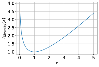
Figure 1: Diversity function apply to each eigenvalues of $\mathbf{C}$.

II-B Feature fusion using an Alternating Projection Algorithm with isotonic contraints

II-B1 Proposed feature fusion methodology

When considering a DeepSAD embedding, denoted as $\mathbf{Y}$, the objective is to determine the optimal combination of these features to construct a health index, denoted as $\mathbf{h}$. For this section, the matrix $\mathbf{Y}$ has to be organized in a sequence corresponding to the order in which samples from the analyzed system were recorded. The time index is represented as $t\in{1,\ldots,T}$.

We propose constructing the HI using an alternating projection algorithm with the objective of finding a HI, denoted $\mathbf{h}\in\mathbb{R}^{T}$, that closely approximates the space of HIs we consider as ideal. This ideal HI space, denoted as ${\rm E}{\rm I}$ and is defined as
$\{{{\rm E}_{\rm I}=\mathbf{z}\mid z_{t}\leq 0\text{ if }t\leq T_{d},z_{t}\geq 1\text{ if }t\geq T_{f},z_{t+1}\geq z_{t}}\}$. In essence, it implies that an ideal HI should have values below 0 when $t$ is less than the time threshold $T_{d}$, representing periods when we assume our samples originate from a healthy system. Conversely, we anticipate the HI to have values above 1 when $t$ exceeds the time threshold $T_{f}$, signifying periods when we consider our samples to come from a degraded system. Furthermore, we expect the HI to exhibit a monotonically increasing trend, capturing changes related to wear rather than shifts in operating conditions. This constraint is referred to as isotonic regression, as introduced in works such as [19, 20], and has recently been applied in [4] for HI denoising. The optimization algorithm involves finding the regressor $\mathbf{w}\in\mathbb{R}^{K}$ such that:

$$\underset{\mathbf{w},\mathbf{z}}{\rm argmin}\hskip 14.22636pt \mid\mid\mathbf{h}-\mathbf{z}\mid\mid_{F}^{2}+\beta{\rm R}(\mathbf{w})$$ (6)

$$\hskip 14.22636pt{\rm s.t.}\hskip 14.22636pt \mathbf{h}=\mathbf{Y}\mathbf{w}$$

$$\mathbf{z}\in{\rm E}_{\rm I}$$

In this context, $\mathbf{z}$ represents an HI that falls within the set ${\rm E}_{\rm I}$, and $\mathbf{R}(\bullet)$, with a hyperparameter $\beta$, acts as a potential regularization function designed to prevent overfitting. This regularization function can take the form of ridge regularization, denoted as $\mathbf{R}(\mathbf{w})=||\mathbf{w}||_{F}^{2}$, but it can also be extended to incorporate lasso or elastic net regularization if the feature space has high dimensionality, denoted as $K$.

II-B2 Algorithm

To address the optimization problem presented in Equation 6, we propose an alternating approach [21], in which we iteratively optimize the regressors $\mathbf{w}$ and the ideal HI $\mathbf{z}$. When optimizing $\mathbf{w}$ while keeping $\mathbf{z}$ fixed, the optimization problem in Equation 6 transforms into the following:

$$\underset{\mathbf{w}}{\rm argmin}\hskip 14.22636pt \mid\mid\mathbf{Y}\mathbf{w}-\mathbf{z}\mid\mid_{F}^{2}+\beta{\rm R}(\mathbf{w})$$ (7)

Depending on the type of regularization used, denoted as ${\rm R}(\mathbf{w})$, this process involves solving a ridge, lasso, or elastic net regression. Conversely, when optimizing $\mathbf{z}$ while keeping $\mathbf{w}$ fixed, the optimization problem in Equation 6 transforms into:

$$\underset{\mathbf{z}}{\rm argmin}\hskip 14.22636pt \mid\mid\mathbf{h}-\mathbf{z}\mid\mid_{F}^{2}$$ (8)

$$\mathbf{z}\in{\rm E}_{\rm I}$$

This step involves directly projecting the HI $\mathbf{h}$ onto the space of the ideal HI. To ensure the HI’s monotonic increase, we perform an isotonic regression, utilizing the Pool Adjacent Violator Algorithm [4, 19] which is notably efficient with a complexity of O(t).

It is worth noting that when $\beta=0$, this process effectively projects the HI simultaneously onto the subspace defined by the features $\mathbf{Y}$ and the space of ideal HIs ${\rm E}_{\rm I}$, as illustrated in Figure 2. However, since the subspace generated by $\mathbf{Y}$ may encompass ${\rm E}_{\rm I}$ in cases where the condition $K<<F$ is not met, this can potentially lead to less relevant solutions that are highly sensitive to the algorithm’s initialization. In such scenarios, the regularization ${\rm R}(\mathbf{w})$ becomes particularly crucial.

The algorithm of the proposed Alternating Projection Algorithm with Isotonic Constraint (APAIC) is presented in Algorithm. 1

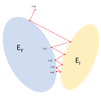
Figure 2: Schematic illustration of the alternating projection algorithm for a 2-D space. $E_{I}$ represents the space of perfect health indicators, while $E_{Y}$ denotes the space generated by the dataset.

Algorithm 1 Algorithm to solve the optimisation problem 6

Dataset $\mathbf{Y}$ and hyperparameter $\beta$

$\mathbf{w}=\mathbf{1}$

for $i\in$ $\{1,...,I\}$ do

     Solve the regression problem equation 7

     $\mathbf{h}=\mathbf{Y}\mathbf{w}$

     $\mathbf{z}=\mathbf{h}$

     $z_{t}=0$ for $t\in\{1,...,T_{d}\}$ if $z_{t}>0$

     $z_{t}=1$ for $t\in\{T_{f},...,T\}$ if $z_{t}<1$

     Perform isotonic projection on $\mathbf{z}$ using the PAVA algorithm [4]

end for

II-B3 Training and real-time HI construction

In practice, our optimization algorithm combines data from both the training and validation datasets with our test dataset. This approach is necessary because it is not feasible for the test dataset to determine the degraded time threshold $T_{f}$, as we construct the HI specifically to estimate it. Therefore, when we denote $\mathbf{Y}^{(v)}$ as $v$ different validation or training datasets, and $\mathbf{Y}_{:t}$ as the first $t$ recorded samples of the investigated system, the optimization problem in Equation 6 transforms into:

$$\underset{\mathbf{w},\{\mathbf{z}^{(1)},..,\mathbf{z}^{(K)}\},\mathbf{z}}{\rm argmin}\hskip 14.22636pt \sum_{k=1}^{K}\mid\mid\mathbf{h}^{(k)}-\mathbf{z}^{(k)}\mid\mid_{F}^{2}+\mid\mid\mathbf{h}_{:t}-\mathbf{z}\mid\mid_{F}^{2}+\beta{\rm R}(\mathbf{w})$$ (9)

$$\hskip 14.22636pt{\rm s.t.}\hskip 14.22636pt \mathbf{h}^{(k)}=\mathbf{Y}^{(k)}\mathbf{w}$$

$$\mathbf{z}^{(k)}\in{\rm E}_{\rm I}$$

$$\mathbf{h}_{:t}=\mathbf{Y}_{:t}\mathbf{w}$$

$$\mathbf{z}\in{\rm E}_{\rm I}^{\rm Test}$$

In this context, ${\rm E}_{\rm I}^{\rm Test}={\{\mathbf{z}\mid z_{t}\leq 0\text{ if }t\leq T_{d},z{t+1}\geq z_{t}\}}$ represents the subset of ideal test HIs, excluding the worn-out condition. To address this optimization problem, Algorithm 1 can be applied. It involves concatenating features and ideal HIs for updating the regressor $\mathbf{w}$, while the projection onto the ideal subspace should be carried out separately for each system.

III Application on a benchmark dataset: The PHME 2010 milling wear datasets

The International Prognostic and Health Management 2010 Challenge (PHM2010) Milling Wear Datasets address the issue of deterioration of milling tools and the continuous tracking of this wear within machining systems. In this section we propose to apply the proposed semi-supervised APAIC merging methodology on the 2DS features for HI prediction. The HI prediction is done here without using the labels provided by the dataset for the training of the models.

III-A Dataset

The PHM2010 dataset originates from a high-speed computerized numerical control machine known as the Röders Tech RFM760. The dataset encompasses data collected from seven distinct sensors, measuring cutting forces, vibration, and acoustic emissions. Data acquisition for each channel occurred at a rate of 50 KHz. Figure 3(a) provides an illustration of the experimental data acquisition platform. A dynamometer was installed between the machine table and the workpiece to measure cutting forces along three directions: x, y, and z. Additionally, three Kistler piezo accelerometers were positioned to monitor machine tool vibrations in the x, y, and z directions. Lastly, a Kistler Acoustic Emission sensor was employed to track high-frequency stress waves, and the data is provided as the root mean square of the acoustic emission. Following each cutting test, an offline measurement of the flank wear depth of the three individual flutes was conducted using a LEICA MZ12 microscope. The maximum wear depth observed serves as a valuable health state indicator for assessing the cutting tool. In total, three milling experiments with ground truth HIs were conducted (denoted as C1, C4, and C6). Figure 3 (b) displays the full trajectories of these three HIs. We perform cyclic rotations of the training, validation, and testing datasets. In the first rotation, C1 is used for training, C4 for validation, and C6 for testing. In the subsequent rotation, we train on the C4 dataset, validate on C6, and test on C1. In the last rotation we train on C6. validate on C1 and test on C4. To ensure robustness, we employed a bootstrapping strategy and present the averaged results across all possible permutations of splitting between the training, validation, and test datasets. For additional information about the system, further details can be found in the references [5], [6], and [8].

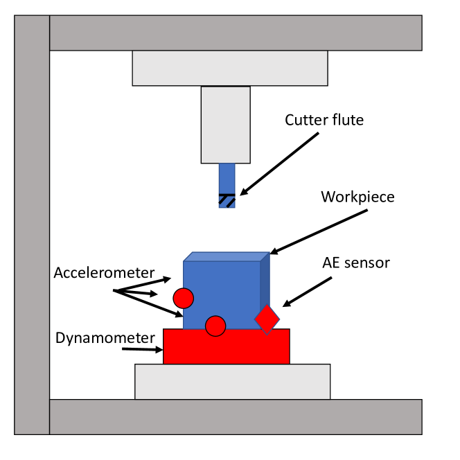
(a)

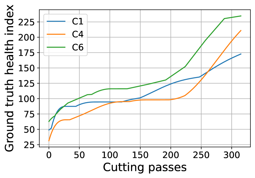
(b)

Figure 3: (a) PHME 2010 data acquisition experimental platform - (b) Ground trouth health index labels for three complete lifecycles dataset

III-B Input features and metrics

For each sensor modality, we transformed the data into a mel spectrogram with 64 channels. We selected a window size of 0.1 seconds and a hop length of 0.1 seconds. The mel spectrograms from all sensor modalities were then merged along the feature dimension to form the input feature vector $\mathbf{x}$ for each time step, resulting in a vector in dimension $F=448$.

The goal of this study is to find a model that map the input feature $\mathbf{X}$ into an estimation $\hat{\mathbf{h}}$ of the ground truth HI obtained through microscopy. We focus on the average HI obtained for each cutting pass. To evaluate the quality of the estimated HI, we employ the following two metrics:

• Correlation: The correlation is important for evaluating the similarity between the shape of our estimated HI and that of the ground truth HI. The correlation score for any trajectory denoted as $c\in\{{\rm c1},{\rm c4},{\rm c6}\}$ is calculated as follows:

  $${\rm Correlation}=\frac{\hat{\mathbf{h}}^{t}\mathbf{h}}{||\hat{\mathbf{h}}||_{F}||\mathbf{h}||_{F}}$$ (10)

• RMSE: The Root Mean Squared Error (RMSE) is used to assess the relationship between the values of different HIs. In particular, if the ground truth HI value for one experiment exceeds the values for another experiment, it should be reflected in the estimated HI. Since our estimated HI values fall within the range of 0 to 1, we rescale them using the following operation:

  $$\hat{\mathbf{h}^{\prime}}=\hat{\mathbf{h}}M+m,$$ (11)

  $$M=\frac{M_{2}-m_{2}}{M_{1}-m_{1}},$$

  $$m=m_{2}-mM,$$

  $$m_{1}={\rm mean}([\hat{\mathbf{h}}^{\rm(c1)}_{100:150},\hat{\mathbf{h}}^{\rm(c4)}_{100:150},\hat{\mathbf{h}}^{\rm(c6)}_{100:150}]),$$

  $$m_{2}={\rm mean}([\mathbf{h^{\rm(c1)}}_{100:150},\mathbf{h^{\rm(c4)}}_{100:150},\mathbf{h^{\rm(c6)}}_{100:150}]),$$

  $$M_{1}={\rm max}([\hat{\mathbf{h}}^{\rm(c1)},\hat{\mathbf{h}}^{\rm(c4)},\hat{\mathbf{h}}^{\rm(c6)}]),$$

  $$M_{2}={\rm max}([\mathbf{h^{\rm(c1)}},\mathbf{h^{\rm(c4)}},\mathbf{h^{\rm(c6)}}]).$$

  Although it may appear complex, this equation essentially ensures that both the ground truth and estimated HIs have identical means during the stationary period from 100 to 150, as well as matching maximum values across the three experiments. This operation simply entails applying the same affine transformation to the three estimated HIs, ensuring that their relative relationships remain unchanged. Consequently, for any experiment denoted as $c\in\{{\rm c1},{\rm c4},{\rm c6}\}$, the RMSE score can be expressed as follows:

  $${\rm RMSE}=||\hat{\mathbf{h}^{\prime}}-\mathbf{h}||_{F}.$$ (12)

III-C Performance of the APAIC merging algorithm

III-C1 APAIC training

Initially, we employ the APAIC algorithm directly on the raw features $\mathbf{X}$ without utilizing the DeepSAD algorithm for condition indicator estimation. For this analysis, we consider the average features for each cutting pass, totaling $T=315$ cutting passes. Subsequently, we proceed to directly determine the regressor $\mathbf{w}$ that satisfies Equation 9 with $t=T=315$. For this purpose, we utilize two trajectories for the training dataset, corresponding to the HIs projected into the space ${\rm E}_{\rm I}$ as described in Equation 9. Conversely, for the test experiment, the HIs are projected into the space ${\rm E}_{\rm I}^{\rm Test}$ since there is no available information regarding the end of life. We set $T_{d}=50$ and $T_{f}=T-50=265$ to emulate a scenario where the expert’s labeling to distinguish between healthy and worn-out parts is uncertain. We use ridge regularisation with $\beta=0.1$. In Figure 4, we provide an example illustrating the various updates to the HI when employing Algorithm 1. The black line represents the initialization when we consider the sum of all features (we subtract the sum of all features after the first cutting pass from it, so it starts at 0). During the initialization phase, the HI is not relevant, in contrast to the final iteration depicted by the red curve. In the end, we obtain an HI that is a monotonically increasing function remaining below 0 for the first 50 iterations and surpassing 1 for the last three iterations. The gradual convergence to the final solution for each iteration is indicated by the color progression, ranging from dark blue to light green.

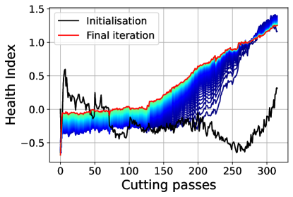
Figure 4: This visualization illustrates the evolution of the APAIC merging algorithm over 1000 iterations on a validation dataset. The algorithm’s progression is depicted through a series of curves, transitioning from blue to green every 10 iterations. The initial state is represented in black, while the final result is highlighted in red.

III-C2 Compared methodologies

We conduct a comparison between our APAIC merging method and another approach that selects the best feature from the pool of 448 available features based on a specified criterion referred to as S1. Here, the feature selection is performed with the aim of choosing the feature that best approximates the ideal feature space ${\rm E}_{\rm I}$ for the two training datasets. Additionally, we compare our method to two oracle procedures, denoted as (O1) and (O2) that select the feature directly according to the test dataset. In case of (O1), our objective is to find the feature that minimizes the correlation score across all three trajectories simultaneously. As for (O2), we directly select the feature that minimizes the correlation for each machine . The Oracle methods (01) and (02) would not be feasible in real application

III-C3 Results

The results for Correlation and RMSE are presented in Table I. Notably, there is a significant disparity in RMSE and correlation scores between the (O1) and (O2) approaches. This discrepancy underscores that distinct features are optimal for predicting the ground truth HI in each trajectories and the same feature may exhibit varying behaviors and scales across different trajectories. As a consequence, the (S1) feature exhibits the poorest performance in terms of RMSE because the features can exhibit different behavior between the training and test datasets.

Finally, we observe that employing the APAIC merging strategy results in both favorable Correlation scores and RMSE scores. We obtain the best RMSE score, which is better than the oracle (O2) selection strategy that uses the test dataset to find the best feature, improving from 25.5 to 24.3. It shows that the APAIC strategy is the most reliable for HI estimation with relevant relationships between each other without access to the test dataset and HI ground truth labels.

	RMSE				Correlation
Method	c1	c4	c6	Mean	c1	c4	c6	Mean
O1 Features	12.91	23.77	54.29	30.33	0.906	0.959	0.910	0.925
O2 Features	28.63	28.43	19.55	25.54	0.964	0.961	0.946	0.957
S1 Features	28.26	29.18	37.04	31.49	0.946	0.951	0.889	0.929
APAIC Features	22.73	29.29	20.84	24.29	0.946	0.885	0.952	0.928

TABLE I: Correlation and adjusted Mean Squared Error (MSE) scores for the Health Index obtained using the APAIC merging method, the Oracle best raw features for all lifecycles based on MSE (O1), the Oracle best raw feature for each lifecycle based on MSE (O2), and the best raw features for each lifecycle obtained based on the S1 criteria.

III-D Performances of combining DeepSAD and APAIC

Based on the findings from the previous experiment, it is evident that using raw features directly for constructing the HI may have limitations. Therefore, our proposed approach first involves using DeepSAD to directly create the HI. We then consider the embedding of DeepSAD as condition indicators related to the health state of the machine. These condition indicators are subsequently merged using the APAIC methodology.

III-D1 DeepSAD training

For DeepSAD training, the final 50 cutting passes from the training dataset are labeled as abnormal samples (label -1 for DeepSAD), while the initial 50 samples are labeled as healthy labels (label 1 for DeepSAD). The remaining samples in the training dataset are considered unlabeled. Furthermore, for training DeepSAD, we include the initial 50 cutting passes from both the validation and test datasets as healthy samples with labels 1. We used the Adam optimizer with a training step size of $5e\text{-}4$ for 1000 epochs, utilizing a batch size of 128. The parameter $\nu$ was fixed at 0.1, and the weight decay $\mu$ was set to 1. We chose this weight decay to ensure consistent results when conducting two simultaneous training sessions of the DeepSAD model with different initial seeds. The DeepSAD model’s architecture comprises a three-layer dense neural network with 32 neurons. We used the ReLU activation function for the first two layers and a linear activation function for the final layer.

III-D2 Proposed approaches and comparison

The APAIC merging strategy is applied to the embedding $\mathbf{Y}$ of the DeepSAD model. Unlike the straightforward utilization of Mel spectrogram features, the embedding $\mathbf{Y}$ encompasses multiple features that should be linked to the system’s health status and can act as condition indicators. The resulting Health Indicator (HI) is derived by applying APAIC to these obtained condition indicators and is referred to as APAIC DeepSAD (ADS). Additionally, we mimic the real-time HI estimation case, where incoming data is recorded on the fly. In this case, Equation 9 is minimized several times for $t\in\{\tau,2\tau,...,T\}$ with a step size of $\tau=30$. The final HI is obtained by concatenating the $\tau$ most recent steps of each computed HI. This real-time variant of our proposed methodology is denoted as ”RADS.” Finally, we explore the scenario in which we train the 2DS model Equation. 3 using a fixed value of $\lambda=0.001$ to employ the diversity loss. This allows us to generate the HI using the ”2DS”, ”A2DS” and ”RA2DS” models. The various terminologies for the proposed approaches are summarized in the Table II

Method name	APAIC	Real-Time	Diversity
	Eq. 9	Eq. 9	loss Eq. 3
DeepSAD	✗	✗	✗
ADS	✓	✗	✗
RADS	✓	✓	✗
2DS	✗	✗	✓
A2DS	✓	✗	✓
RA2DS	✓	✓	✓

TABLE II: Terminology for the various methods

For comparison with an unsupervised setting, we introduce a one-class classifier, the Support Vector Data Description (SVDD) [22]. We consider the radial basis function kernel and empirically tune the hyperparameters $C$ and $\gamma$ based on the validation dataset, selecting the parameter combination that results in an estimated HI minimizing the distance from the ideal HI space ${\rm E}_{\rm I}$.

III-D3 Results

Table III displays the results comparing all methods. It is evident that DeepSAD alone outperforms SVDD for both metrics but is surpassed by the ”ADS” method, resulting in a significant improvement in both correlation and RMSE scores. Indeed, employing ADS leads to a reduction in RMSE from 27.7 to 18.4.

The diversity regularisation improves performance when using both the norm of the embedding directly as HI and when employing the APAIC merging strategy on the 2DS embeddings. It does appear to provide enriched condition indicators that aid the APAIC procedure in finding more refined HIs. The ”A2DS” method maintains a very high correlation score, similar to ”ADS”, with both achieving up to 0.970. However, it also reduces the RMSE from 18.2 to 13.9. This improvement is primarily attributed to a more accurate prediction of the ”c4” HI values, where the RMSE is reduced from 27.8 to 14.2. Finally, it is worth noting that in the real-time scenario, both ”RADS” and ”RA2DS” offer similar scores overall.

Figure 5 presents the obtained HI for the three milling machines along with their respective ground truth HIs indicated by dotted lines. It demonstrates that the DeepSAD models primarily emphasize the regions associated with severe wear, while the APAIC merging methods reveal more complex trajectories. As shown in the Table III, the best fit is achieved with the ”RA2DS” strategy, where we observe both a strong correlation between the HI and a good alignment between the estimated HI values and the ground truth.

For more ablation studies showing the impact of $\beta$ and the isotonic constraint in Equation 9, the impact of $\lambda$ in equation Equation 3 and the impact of the embedding size for ADS, please refer to A.

	RMSE				Correlation
Method	c1	c4	c6	Mean	c1	c4	c6	Mean
S1 Features	28.26	29.18	37.04	31.49	0.946	0.951	0.889	0.929
APAIC Features	22.73	29.29	20.84	24.29	0.946	0.885	0.952	0.928
SVDD	18.90	31.65	43.65	31.40	0.844	0.744	0.792	0.793
DeepSAD	17.66	21.04	44.46	27.72	0.908	0.947	0.889	0.915
ADS	8.06	27.80	18.87	18.24	0.969	0.971	0.977	0.972
RADS	10.83	31.73	15.76	19.44	0.964	0.971	0.978	0.971
2DS	13.46	20.48	37.02	23.65	0.907	0.938	0.847	0.897
A2DS	9.70	14.17	17.97	13.94	0.967	0.970	0.980	0.972
RA2DS	7.14	14.70	19.04	13.63	0.968	0.980	0.978	0.975

TABLE III: Correlation and adapted RMSE for the Health Index (HI) obtained using various methods

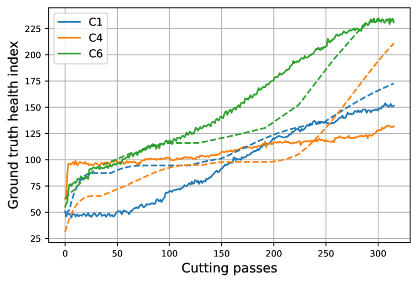
(a)

(b)

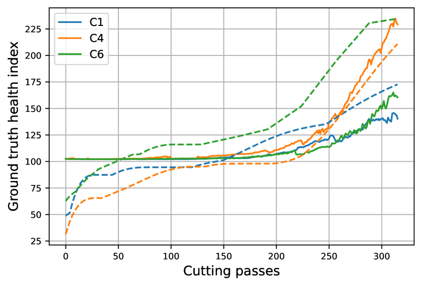
(c)

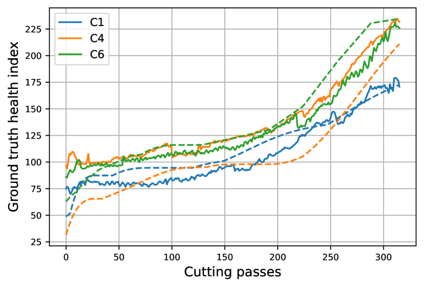
(d)

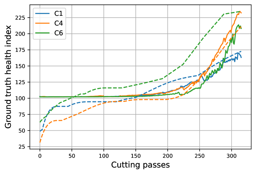
(e)

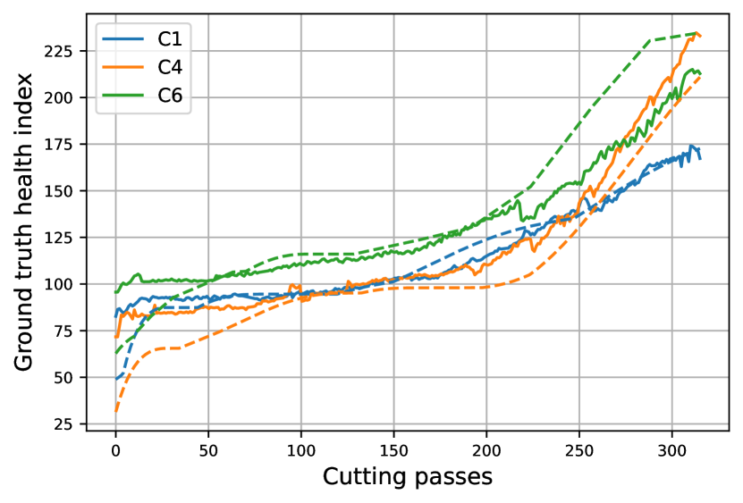
(f)

Figure 5: Comparison between the estmated (solid line) and ground truth (dotted) for the following methods (a) APAIC Feature (b) SVDD (c) DeepSAD (d) RADS (e) 2DS (f) RA2DS

III-E Comparison against supervised model

The milling dataset, which includes ground truth HI, is widely regarded as an ideal dataset for supervised HI prediction. As a result, the majority of previous studies on this dataset utilized these labels to train various machine learning models[9, 23, 24, 25, 26]. In our work, we take a different approach by not using the ground truth HI for training and instead approximating labels. To provide a more relevant comparison, we focus on a recent study [6], which aligns with our work. This study utilizes data from all sensors and employs similar input features, specifically the Wavelet Packet Transform node output for each sensor modality.

Table IV presents the results obtained from various supervised methods as compared in [6]. The correlation metric was not computed in the mentioned study. We focus on our best-performing approach, which is the RA2DS. Our semi-supervised approach demonstrates performance comparable to the top-performing supervised methods, only being surpassed by the stacked sparse AE proposed in [6] approach, which achieved an RMSE score of 12.7, while our approach yielded a score of 13.6.

	RMSE
Method	c1	c4	c6	Mean
MLP	28.8	39.8	33.6	34.07
CNN	29.3	43.6	55.3	42.73
LSTM	11.4	11.7	21.2	14.43
RNN	15.6	19.7	32.9	22.73
BLSTM	12.3	14.7	20.8	15.93
Sparse Stacked AE	9.3	14.0	14.8	12.70
RA2DS (semi-supervised)	7.14	14.70	19.04	13.63

TABLE IV: Comparison of our semi-supervised approach with supervised methods that use ground truth labels for training.

IV Application to spray coating monitoring

In addition to the benchmark dataset evaluation, we also evaluate the proposed methodology on a real-world application: estimate the health condition of thermal spray for high quality surfaces coating. Thermal spray (TS) is an advanced technology used to efficiently coat surfaces and alter their mechanical and thermal properties. Some of the most common TS coating technologies include plasma spray, high-velocity oxy-fuel (HVOF), and Arc spray. Systems to which thermal spray coating is typically applied include jet engines, gas turbines, and automobile systems. Since these systems are safety-critical and mission-critical, coating quality is of significant importance.

Amongst all TS technologies, Atmospheric Plasma Spray (APS) is the most versatile and widely used method capable of spraying a wide range of materials onto various substrate materials. The spray gun is the most critical component of the plasma spray coating system, and the nozzle-electrode pair is the most crucial part of the plasma spray gun. Currently, there is a lack of suitable tools that can monitor the quality and process stability of thermal spray coatings. The APS process is characterized by several parametric drifts and fluctuations occurring at different time scales. These phenomena stem from various sources, including electrode wear and intrinsic plasma jet instabilities, as well as powder feeder fluctuations. In fact, the condition of the nozzle-electrode pair is important factor affecting the coating quality characteristics of plasma spray.

There has been limited research on the analysis of signals recorded during the coating process to monitor fluctuations in the thermal spray process. In a study conducted by [27], the HVOF process was investigated by collecting and analyzing airborne acoustic emissions (AAE) within the booth. This study relied on features extracted using FFT and was not tested with data from other guns of the same hardware or with different hardware and parameters. It was based on a very limited dataset from a single gun with specific hardware and parameters. Furthermore, it provided an estimation of the current process state but could not be used for predictions. In another study by [28], an offline method was developed to determine the wear state of GH-type nozzles for Oelikon Metco 9MB plasma spray guns. This was achieved by recording and analyzing the acoustic signals generated by a controlled gas flow through each nozzle.

In this paper, we address the challenge of monitoring the health state and lifetime of the nozzle/electrode without requiring modifications to the spraying system (non-intrusive) and without disrupting the production plan (non-disruptive). Our approach involves extracting relevant features from the High Frequency (HF) gun voltage signal during the coating process to assess the health state and lifetime of the gun nozzle and electrode. Typically, the lifetime of a nozzle ranges from 10 to 40 hours, depending on the stress imposed on the nozzle by the arc energy. The condition of the nozzle significantly impacts coating quality. The objective is to estimate the nozzle’s state in real-time and recommend the optimal time for nozzle replacement to achieve both the coating quality requirements and maximum hardware utilization.

IV-A Dataset

We collected high-frequency gun voltage for identifying nozzle wear. While plasma spray guns operate on direct current, the voltage fluctuates rapidly. These fluctuations and the mean voltage change with nozzle degradation. The condition monitoring system primarily employs a high frequency voltage sensor is used to record gun voltage generated by the thermal spray gun during operation. The data is stored, converted into a readable format, and then processed. The signal is further connected to a high frequency DAQ (Data Acquisition System) for digital conversion.

The sampling frequency was set to 50 kHz. We used an Oerlikon Metco F4 gun, with a 6mm nozzle, and recorded gun voltage for throughout the nozzle’s lifetime for 4 nozzle-electrode pairs. Nozzle’s lifetime varies depending on several controlled and uncontrolled conditions, such as nozzle/electrode installation differences, gun setup, water temperature and more. In the experiments, we used 45/10.5 NLPM Ar/H2 with 650 A of current. We conducted incremental testing on the nozzles over a period of 15 to 45 hours of operation, assessing when the nozzle reached a “very worn” condition with the assistance of a domain expert. A significant amount of hydrogen was employed to accelerate nozzle/electrode wear due to its constriction of the plasma core, resulting in higher energy density. We convert the high-frequency voltage signal into a Melspectrogram for feature extraction.

IV-B Results

Since we lack the ground truth, we propose employing alternative metrics in this section to evaluate the quality of our HI. The first metric measures the delay between the fault’s onset time and when our estimated HI first reaches a value of 1, which we refer to as the ”Delay.” The second metric we employ is the Root Sum of Square Error (RSSE) calculated between the derived HIs and a HI constructed based on the real binary alarm profile. This constructed ground truth HI linearly increase from 0 to 1 until the fault’s onset time, after which it remains constant at 1 until the end of the experiment. We cap the HI values at 1 for this specific metric to avoid penalizing HIs that could potentially exceed 1. The ”Delay” score serves as a local metric, assessing our HI’s ability to assess the end of life. Conversely, the RSSE score serves as a global metric, evaluating the overall quality of our HI’s shape.

We conducted a comparison among three methods: the DeepSAD model, the RADS, and the RA2DS. For RADS and RA2DS we consider a step size $\tau$ of 4 hours. We maintained consistent hyperparameters with the previous benchmark dataset and set $\lambda$ to a fixed value of 0.1. For both the DeepSAD and APAIC algorithms, we classified samples from the first 5 hours of machine operation as healthy. Conversely, we labeled samples recorded after the fault’s onset time as abnormal.

Tables V and VI present the Delay and RMSE scores for all four nozzles. DeepSAD failed to trigger alarms in nozzle two and three while RADS failed to trigger an alarm in nozzle four. RA2DS was able to detect the end of life for all four nozzles. On average, when an alarm was triggered, RA2DS exhibited the closest detection time to the fault onset, with an average delay of 1.4 hours. In contrast, RADS had an average alarm delay of 3.6 hours, and DeepSAD displayed an alarm delay of 7.8 hours. Regarding the RSSE scores, once again, RA2DS outperformed the other methods, with an average score of 12.7 and the DeepSAD model displayed the poorest performance with a score of 17.6.

Figure 7 shows the obtained HIs for each nozzle, with the expert binary labels represented in black. Among the four experiments, RA2DS stands out as the most reliable HI. It has a consistent evolution between 0 and 1. We cannot further assess the relevance of the obtained HI since we do not have access to the ground truth HI. Nevertheless, this score can be employed to evaluate the wear level, with the goal of estimating the remaining useful life, triggering an alarm before the nozzle reaches a worn-out state, or extending the use of a nozzle if the associated health index remains low even after the typical replacement time.

	Delay
Method	N1	N2	N3	N4	Mean
DS	8.62	-	-	6.948	7.784
RADS	8.55	2.02	0.33	-	3.632
RA2DS	2.50	2.83	0.10	0.086	1.379

TABLE V: The ”Delay” represents the time between the fault’s estimated onset and the alarm raised by our estimated HI. A ”-” indicates that no alarms were raised during that period.

	RSSE
Method	N1	N2	N3	N4	Mean
DS	13.74	23.80	26.86	5.962	17.588
RADS	9.05	10.39	16.23	26.204	15.466
RA2DS	15.03	11.88	16.40	7.588	12.724

TABLE VI: The RSSE (Root Sum Square Error) is calculated between the synthetic ground truth and the estimated HI for each compared method. The HIs are adjusted to ensure they are capped at 1 during this analysis..

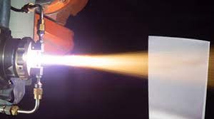
(a)

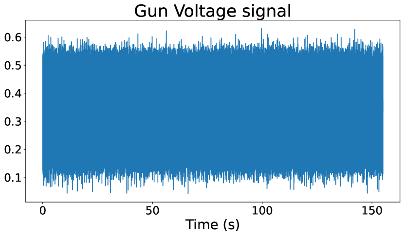
(b)

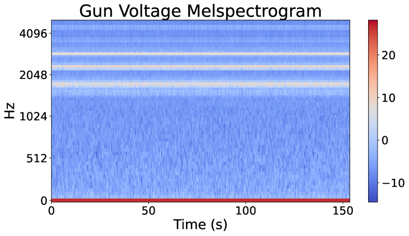
(c)

(d)

Figure 6: (a) Spray coating system - (b) High frequency volage signal - (c)-(d) Melspectrogram of the voltage signal repsectively at the begin and the end of the lifecycle.

(a)

(b)

(c)

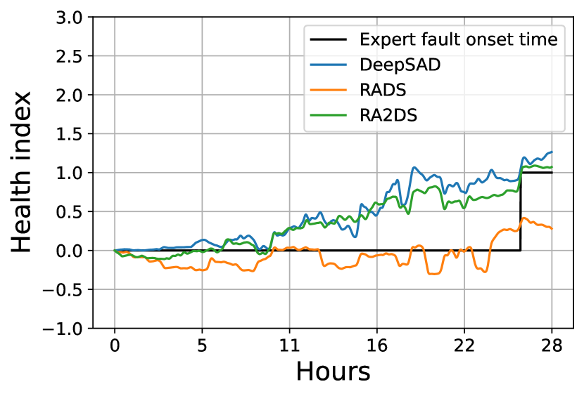
(d)

Figure 7: Comparison between estimated DeepSAD, ADS, A2DS HIS and binary alarm estimated by experts for the 4 nozzles lifecycles.

V Conclusion

In this study, we introduced an HI construction method based on a semi-supervised anomaly detection approach called DeepSAD. Contrary to fully supervised approach where we need a measure of the real health state of the machine, which can be prohibitively expensive or impractical in real-world applications. Often, it is only feasible to acquire labels for the beginning or end of a system’s lifecycle through available data. Indeed, there are healths states that are easier to assess: when the system is new and can be assumed to be healthy, or when the system fail and we are sure it is degraded. Thus, we propose a semi-supervised approach for HI construction. Our approach involves enhancing the DeepSAD embedding to generate condition indicators associated with various wearing within the system. These indicators are then integrated to create the HI using a novel alternating projection algorithm that ensures a normalized and monotonically increasing HI.

We evaluated the robustness of our approach using the PHME 2010 milling dataset, a benchmark dataset with ground truth HI values. Our findings demonstrate that our approach not only produces HIs that correlate with ground truth data but also ensures that the estimated HI values correspond to the relative wear states of different machines. Furthermore, we evaluate the applicability our approach to a real-world application, monitoring the wear states of thermal spray coatings with high-frequency voltage sensors. Our results indicate that our method yields HIs that consistently increase when expert detect that the system approaches the end of life.

Potential future directions for this research include exploring the application of the APAIC algorithm for feature merging in scenarios involving high-dimensional features or data from different modalities. Another avenue of investigation involves combining the APAIC and DeepSAD models into an end-to-end learning approach for the direct estimation of a robust HI.

Aknowledgments

This study was financed by the Swiss Innovation Agency (lnnosuisse) under grant number: 47231.1 IP-ENG.

We would like to express our gratitude to Ehsan Fallahi for carrying out the data collection for the spray coating application, and Ron Molz for his expert opinion on data analysis and labeling the data.

Appendix A Ablation study

This section relate to the same experiments as in Section III-D. We study the influence of the different hyper-parameters from the ADS and A2DS methodology.

A-A Impact of the parameters of APAIC

We explore the ADS methodology for different values of $\beta$ in Equation 9 using the Ridge regularization. We also study the presence or absence of the Isotonic constraint. The results are presented in Table VII. We can see that without both the Ridge regularisation ($\beta=0$) and the Isotonic constraint the algorithm does not succeed to converge. Overall the results are stable for different values of $\beta$ with exactly the same correlation score and fairly similar RMSE score.

A-B Impact of the size of the embedding $K$ in DeepSAD

We investigate the embedding size of DeepSAD, denoted as $\mathbf{Y}\in\mathbb{R}^{F\times K}$, for various values of $K$. The results are presented in Table VIII. Once more, the results remain stable regardless of the value of this hyperparameter. The best RMSE value is achieved when $K=64$, however, it is associated with the lowest correlation score.

A-C Impact of the diversity parameters $\lambda$ in 2DS

We examine the impact of the diversity regularization parameter $\lambda$ as defined in Equation 3. The outcomes are displayed in Table IX. For values of $\lambda$ greater than or equal to 0.01, we select the results with the lowest loss after five different initializations, as the algorithm yields varied results depending on the initialization. We defer the investigation of this issue for future research. It seems that the value of $\lambda$ needs to be carefully balanced. When it becomes too high, the parameters of the DeepSAD model become negligible in comparison to the diversity loss, which results in trajectories that cannot be considered as reliable condition indicators. The value $\lambda=0.001$ corresponds to a balancing parameter that aligns the magnitudes of the DeepSAD model loss and diversity loss for this experiment.”

In Figure 8, we present the absolute embeddings acquired from the test dataset c6 for four distinct values of $\lambda$. In the case of $\lambda=0$, most trajectories display precisely the same pattern. As we introduce $\lambda=0.001$, some condition indicators activate at different times, yielding more diverse patterns. When $\lambda=1$, the embedding exhibits varying activation periods, effectively segmenting the time axis into different clusters. Although these diverse trajectories hold potential for future investigations, they appear noisier and more challenging to integrate for the APAIC algorithm.

(a)

(b)

(c)

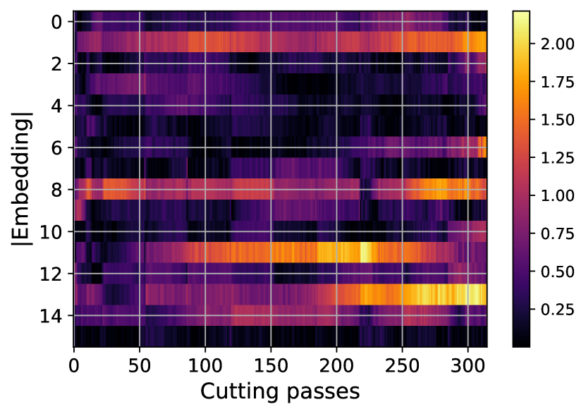
(d)

Figure 8: Absolute value of the lifecycle embedding obtained for the test c1 dataset for different diversity regularisation(a) 0 (b) 0.001 (c) 0.01 (d) 1

$\beta$	Isotonicity	RMSE				Correlation
		c1	c4	c6	Mean	c1	c4	c6	Mean
$\beta=0$	no	147.33	96.25	145.28	129.62	-0.514	-0.791	-0.639	-0.648
$\beta=0$	yes	26.73	30.97	16.58	24.76	0.979	0.897	0.962	0.946
$\beta=0.001$	yes	7.77	30.40	17.23	18.47	0.969	0.971	0.977	0.972
$\beta=0.01$	yes	7.41	29.88	17.49	18.26	0.969	0.971	0.977	0.972
$\beta=0.1$	yes	7.83	28.28	18.66	18.26	0.969	0.971	0.977	0.972
$\beta=1$	no	8.92	27.88	18.99	18.60	0.969	0.971	0.977	0.972
$\beta=1$	yes	8.06	27.80	18.87	18.24	0.969	0.971	0.977	0.972

TABLE VII: Impact of the Isotonic constraint and Ridge regularisation hyperparameter $\beta$

	RMSE				Correlation
Dimension	c1	c4	c6	Mean	c1	c4	c6	Mean
8	14.52	29.11	15.87	19.83	0.963	0.968	0.969	0.967
16	8.06	27.80	18.87	18.24	0.969	0.971	0.977	0.972
32	18.33	15.17	26.21	19.90	0.969	0.965	0.975	0.970
64	10.39	22.59	12.24	15.07	0.953	0.962	0.975	0.964

TABLE VIII: Impact of the dimension of the ADS embedding

	RMSE				Correlation
$\lambda$	c1	c4	c6	Mean	c1	c4	c6	Mean
$\lambda$ =0	8.06	27.80	18.87	18.24	0.969	0.971	0.977	0.972
$\lambda$ =0.001	9.70	14.17	17.97	13.94	0.967	0.970	0.980	0.972
$\lambda$ =0.01	10.91	24.06	13.74	16.23	0.966	0.962	0.970	0.966
$\lambda=1$	9.60	19.77	30.99	20.12	0.966	0.928	0.891	0.928

TABLE IX: Impact of the dimension of the Diversity regularisation

References

- [1] O. Fink, Q. Wang, M. Svensen, P. Dersin, W.-J. Lee, M. Ducoffe, Potential, challenges and future directions for deep learning in prognostics and health management applications, Engineering Applications of Artificial Intelligence 92 (2020) 103678.
- [2] G. Michau, T. Palm, O. Fink, Deep feature learning network for fault detection and isolation, in: Annual Conference of the PHM Society, Vol. 9, 2017.
- [3] C.-C. Hsu, G. Frusque, O. Fink, A comparison of residual-based methods on fault detection, arXiv preprint arXiv:2309.02274 (2023).
- [4] H. Wang, H. Liao, X. Ma, R. Bao, Remaining useful life prediction and optimal maintenance time determination for a single unit using isotonic regression and gamma process model, Reliability Engineering & System Safety 210 (2021) 107504.
- [5] X. Li, B. Lim, J. Zhou, S. Huang, S. Phua, K. Shaw, M. Er, Fuzzy neural network modelling for tool wear estimation in dry milling operation, in: Annual Conference of the PHM Society, Vol. 1, 2009.
- [6] Z. He, T. Shi, J. Xuan, Milling tool wear prediction using multi-sensor feature fusion based on stacked sparse autoencoders, Measurement 190 (2022) 110719.
- [7] W. Li, H. Fu, Z. Han, X. Zhang, H. Jin, Intelligent tool wear prediction based on informer encoder and stacked bidirectional gated recurrent unit, Robotics and Computer-Integrated Manufacturing 77 (2022) 102368.
- [8] W. Liu, W.-A. Yang, Y. You, Three-stage wiener-process-based model for remaining useful life prediction of a cutting tool in high-speed milling, Sensors 22 (13) (2022) 4763.
- [9] C. Zhou, W. Wang, Z. Hou, W. Feng, Milling cutter wear prediction based on bidirectional long short-term memory neural networks, in: ISMSEE 2022; The 2nd International Symposium on Mechanical Systems and Electronic Engineering, VDE, 2022, pp. 1–6.
- [10] X. Jin, H. Pan, C. Ying, Z. Kong, Z. Xu, B. Zhang, Condition monitoring of wind turbine generator based on transfer learning and one-class classifier, IEEE Sensors Journal 22 (24) (2022) 24130–24139.
- [11] Q. Chao, Y. Shao, C. Liu, X. Yang, Health evaluation of axial piston pumps based on density weighted support vector data description, Reliability Engineering & System Safety 237 (2023) 109354.
- [12] G. Frusque, D. Mitchell, J. Blanche, D. Flynn, O. Fink, Non-contact sensing for anomaly detection in wind turbine blades: A focus-svdd with complex-valued auto-encoder approach, arXiv preprint arXiv:2306.10808 (2023).
- [13] L. Ruff, R. A. Vandermeulen, N. Görnitz, A. Binder, E. Müller, K.-R. Müller, M. Kloft, Deep semi-supervised anomaly detection, arXiv preprint arXiv:1906.02694 (2019).
- [14] T. DeLise, Deep semi-supervised anomaly detection for finding fraud in the futures market, arXiv preprint arXiv:2309.00088 (2023).
- [15] Z. Pan, Z. Meng, Z. Chen, W. Gao, Y. Shi, A two-stage method based on extreme learning machine for predicting the remaining useful life of rolling-element bearings, Mechanical Systems and Signal Processing 144 (2020) 106899.
- [16] Z. Chen, D. Zhou, E. Zio, T. Xia, E. Pan, A deep learning feature fusion based health index construction method for prognostics using multiobjective optimization, IEEE Transactions on Reliability (2022).
- [17] J. Friedman, T. Hastie, R. Tibshirani, Sparse inverse covariance estimation with the graphical lasso, Biostatistics 9 (3) (2008) 432–441.
- [18] G. Frusque, J. Jung, P. Borgnat, P. Gonçalves, Regularized partial phase synchrony index applied to dynamical functional connectivity estimation, in: ICASSP 2020-2020 IEEE International Conference on Acoustics, Speech and Signal Processing (ICASSP), IEEE, 2020, pp. 5955–5959.
- [19] D.-I. Tang, S. P. Lin, Extension of the pool-adjacent-violators algorithm, Communications in statistics-theory and methods 20 (8) (1991) 2633–2643.
- [20] A. Lanza, L. Di Stefano, Statistical change detection by the pool adjacent violators algorithm, IEEE transactions on pattern analysis and machine intelligence 33 (9) (2011) 1894–1910.
- [21] R. Escalante, M. Raydan, Alternating projection methods, SIAM, 2011.
- [22] D. M. Tax, R. P. Duin, Support vector data description, Machine learning 54 (2004) 45–66.
- [23] C. Gao, S. Bintao, H. Wu, M. Peng, Y. Zhou, New tool wear estimation method of the milling process based on multisensor blind source separation, Mathematical Problems in Engineering 2021 (2021) 1–11.
- [24] Q. Wu, X. Zhou, X. Pan, Cutting tool wear monitoring in milling processes by integrating deep residual convolution network and gated recurrent unit with an attention mechanism, Proceedings of the Institution of Mechanical Engineers, Part B: Journal of Engineering Manufacture 237 (8) (2023) 1171–1181.
- [25] H. Liu, Z. Liu, W. Jia, D. Zhang, Q. Wang, J. Tan, Tool wear estimation using a cnn-transformer model with semi-supervised learning, Measurement Science and Technology 32 (12) (2021) 125010.
- [26] K. Zhang, H. Zhu, D. Liu, G. Wang, C. Huang, P. Yao, A dual compensation strategy based on multi-model support vector regression for tool wear monitoring, Measurement Science and Technology 33 (10) (2022) 105601.
- [27] S. Kamnis, K. Malamousi, A. Marrs, B. Allcock, K. Delibasis, Aeroacoustics and artificial neural network modeling of airborne acoustic emissions during high kinetic energy thermal spraying, Journal of Thermal Spray Technology 28 (2019) 946–962.
- [28] T. Blair, G. Pickrell, R. Batra, M. Cybulsky, R. Sinatra, Offline acoustic plasma spray nozzle wear state and characteristic identification, in: ITSC2015, ASM International, 2015, pp. 612–615.